Universal Trade-off Between Irreversibility and Relaxation Timescale

Abstract

We establish a general lower bound for the entropy production rate based on the Kullback-Leibler divergence and the Logarithmic-Sobolev constant that characterizes the time-scale of relaxation. This bound can be considered as an enhanced second law of thermodynamics. As a crucial application, we find a universal trade-off relation between the dissipation rate and relaxation timescale in thermal relaxation. Importantly, we show that a thermodynamic upper bound on the relaxation time between two given states follows directly from the trade-off relation, serving as an inverse speed limit throughout the entire time region. Our findings unveil some hidden universal behaviors of thermal relaxation processes, which can also be extended to open quantum systems.

Introduction.—The past twenty years have seen extraordinary progress in nonequilibrium statistical physics of small systems with nonnegligible fluctuations. Significant advances include the celebrated fluctuation theorems Jarzynski (1997); Evans et al. (1993); Evans and Searles (1994); Crooks (1999); Jarzynski and Wójcik (2004); Esposito et al. (2009); Esposito and Van den Broeck (2010a); Verley and Lacoste (2012); Verley et al. (2012); Collin et al. (2005); Wang et al. (2002); Koski et al. (2014) containing all information of the stochastic entropy production, speed limit in quantum and classical systems Shiraishi et al. (2018); Cao et al. (2023); Falasco and Esposito (2020); García-Pintos et al. (2022); Hamazaki (2022); Van Vu and Saito (2023a); Lee et al. (2022); Van Vu and Saito (2023b), some refined versions of the second law of thermodynamics Pigolotti et al. (2017); Neri et al. (2017); Shiraishi and Saito (2019); Neri (2020); Van Vu and Hasegawa (2021a, b); Roldán et al. (2015) and the recently proposed thermodynamic uncertainty relations Barato and Seifert (2015); Gingrich et al. (2016); Horowitz and Gingrich (2017); Cao et al. (2020); Dechant and Sasa (2021a); Dechant and Sasa (2021b); Das et al. (2022); Bao and Hou (2023); Manikandan et al. (2020); Gingrich and Horowitz (2017); Cao et al. (2022). Thermodynamic irreversibility, typically quantified by entropy production (rate), is the key to most of the important theorems and relations mentioned above. Transient processes are common in nature and internally out-of-equilibrium, which have not been studied sufficiently enough compared to stationary processes Lapolla and Godec (2020). Fundamental principles governing the thermodynamic irreversibility in transient processes are still lacking and to be explored.

Our main focus here is the crucial and nontrivial class of transient process known as thermal relaxation, which is a fundamental class of physical processes that is ubiquitous in the real world and has many applications in different fields Meibohm and Esposito (2023). Interestingly, thermal relaxation phenomena are complex and varied even under Markov approximations. Typical examples are dynamical phase transitions Meibohm and Esposito (2022, 2023), anomalous relaxation like Mpemba effect Lu and Raz (2017) and asymmetric relaxation from different directions Lapolla and Godec (2020); Manikandan (2021); Van Vu and Hasegawa (2021c). One of the central quantities in thermal relaxation is its time-scale of convergence, which has been intensively studied. A well-developed theory on that is the spectral gap theory, which says that the relaxation time-scale is typically characterized by the spectral gap of the generator of dynamics in the large time regime. Around the spectral gap, some important frameworks on metastability Biroli and Kurchan (2001); Rose et al. (2016); Macieszczak et al. (2016); Mori (2021); Macieszczak et al. (2021) and Mpemba effect Lu and Raz (2017); Klich et al. (2019); Kumar and Bechhoefer (2020); Santos and Prados (2020); Gal and Raz (2020); Baity-Jesi et al. (2019); Carollo et al. (2021); Busiello et al. (2021a); Manikandan (2021) have been established, which mainly focus on the large time limit. However, there are much fewer works concentrating on the entire time region of relaxation processes Mori and Shirai (2022). In particular, general relations between the relaxation timescale and thermodynamic irreversibility that can hold any time in relaxation processes remain unclear.

Here in this letter, we propose a general lower bound for irreversibility based on Kullback-Leibler (KL) divergence and Logarithmic-Sobolev (LS) constant, which is strengthened compared to the standard second law of thermodynamics. The general bound is then applied to thermal relaxation, revealing an intrinsic trade-off relation between the relaxation time-scale and entropy production rate, which works throughout the whole relaxation process, not limited to the large time region. A key application of the trade-off relation is the establishment of a thermodynamically relevant upper bound of the transformation time between any pair of given states during thermal relaxation, which we refer to as the inverse speed limit. We expect that the trade-off relation and the inverse speed limit can be verified by experiments and further utilized to estimate the entropy production rate and transformation time. Moreover, our results may also aid in the design of rapid relaxation processes, which are desirable in numerous situations Carollo et al. (2021).

A general lower bound for entropy production rate.—We are considering a system with $N$ states coupled to a heat bath with inverse temperature $\beta=1/(k_{B}T)$, though the generalization of our results to multiple heat baths is straightforward. The dynamics of the probability of the system to be in state $i$ at time $t,$ $p_{i}(t)$, is described by a master equation

$$\frac{\text{d}}{\text{d}t}p_{i}(t)=\sum_{j=1}^{N}\left[k_{ij}(t)p_{j}(t)-k_{ji}(t)p_{i}(t)\right],$$ (1)

where $k_{ij}(t)$ denotes the transition rate from state $j$ to state $i$ at time $t$. The master equation can be rewritten in a more compact matrix form as $\frac{\text{d}}{\text{d}t}\boldsymbol{p}(t)=\mathcal{L}(t)\boldsymbol{p}(t)$, where $\boldsymbol{p}(t)=[p_{1}(t),p_{2}(t),...,p_{N}(t)]^{\text{T}}$ and

$$\mathcal{L}_{ij}(t)=k_{ij}(t)-\delta_{ij}\sum_{l}k_{li}(t)$$ (2)

is the stochastic matrix (strictly speaking, $\mathcal{L}$ is an operator) at time $t$. The stochastic matrix changes in time due to external protocols. In this letter, we are focused on both cases when the detailed balance condition $k_{ij}(t)\pi_{j}^{t}=k_{ji}(t)\pi_{i}^{t}$ holds for all pairs of $i$, $j$ at any time $t$ or not, wherein $\pi_{i}^{t}$ is the (instantaneous) stationary distribution at time $t$ for state $i$. We denote $\boldsymbol{\pi}_{t}=[\pi_{1}^{t},...,\pi_{N}^{t}]^{\text{T}}$, in which $\boldsymbol{\pi}_{t}$ is defined as the stationary state will be reached if the stochastic matrix is frozen at time $t$. When the detailed balance condition holds, $\boldsymbol{\pi}_{t}$ will be an (instantaneous) equilibrium distribution $\boldsymbol{p}_{t}^{\text{eq}}$ whose entries are $p_{t,i}^{\text{eq}}=e^{-\beta E_{i}(t)}/Z$, with $E_{i}(t)$ being the instantaneous energy of state $i$ at time $t$ and $Z$ the normalization constant. The KL divergence, which is a quantifier of the difference between two probability distribution, is defined as $D[\boldsymbol{p}^{a}||\boldsymbol{p}^{b}]\equiv\sum_{i}p_{i}^{a}\ln(p_{i}^{a}/p_{i}^{b})$. For any Markov jump processes obeying the master equation (1) with an instantaneous equilibrium distribution $\boldsymbol{p}_{t}^{\text{eq}}$ at time $t$, it can be demonstrated that [sketch of the proof is at the end of this letter, see supplemental material (SM) for details of the derivation]

$$\frac{\text{d}}{\text{d}\tau}D[\boldsymbol{p}(\tau)||\boldsymbol{p}_{t}^{\text{eq}}]|_{\text{$\tau=t$}}\leq-4\lambda_{\text{LS}}(t)D[\boldsymbol{p}(t)||\boldsymbol{p}_{t}^{\text{eq}}],$$ (3)

where $\lambda_{\text{LS}}(t)$ is a positive real number determined by $\mathcal{L}(t)$. Further, without detailed balance condition, we still have a similar inequality $\frac{\text{d}}{\text{d}\tau}D[\boldsymbol{p}(\tau)||\boldsymbol{\pi}_{t}]|_{\text{$\tau=t$}}\leq-2\lambda_{\text{LS}}(t)D[\boldsymbol{p}(t)||\boldsymbol{\pi}_{t}]$, where a factor $1/2$ is multiplied on the right hand side (see SM for details). Before proceeding, we denote $\langle f,g\rangle_{\pi}\equiv\sum_{i}fg_{i}^{\dagger}\pi_{i}$ the inner product induced by the stationary distribution $\boldsymbol{\pi}$ (may be instantaneous).

The positive real number $\lambda_{\text{LS}}(t)$ in Eq. (3) is the LS constant Giné et al. (2006) corresponding to the stochastic matrix $\mathcal{L}(t)$, whose definition is given by

$$\lambda_{\text{LS}}\equiv\inf_{\text{Ent}(f)\neq 0}\frac{\text{Re}\langle-\mathcal{L}f,f\rangle_{\pi}}{\text{Ent}(f)},$$ (4)

where $\text{Ent}(f)$ is an entropy-like quantity defined as $\text{Ent}(f)=\sum_{i=1}^{N}|f_{i}|^{2}\ln\left(\frac{|f_{i}|^{2}}{\langle f,f\rangle_{\pi}}\right)\pi_{i}$ and $f$ is any function in the state space of the system. As is shown below, the LS constant is closely connected with relaxation timescale.

According to the standard stochastic thermodynamics, the average entropy production rate $\dot{\sigma}(t)$ at time $t$ in this system is ($k_{B}$ is set to be $1$) Seifert (2012)

$$\dot{\sigma}(t)= \dot{\sigma}_{\text{sys}}+\dot{\sigma}_{\text{m}}$$

$$= \sum_{i,j}k_{ij}(t)p_{j}(t)\ln\frac{k_{ij}(t)p_{j}(t)}{k_{ji}(t)p_{i}(t)},$$ (5)

where $\dot{\sigma}_{\text{sys}}=\sum_{i}\dot{p}_{i}\ln p_{i}$ and $\dot{\sigma}_{\text{m}}=\beta\sum_{i}\dot{p}_{i}E_{i}(t)$ are the change rate of the system entropy and medium entropy respectively. If the stochastic matrix always satisfies the detailed balance condition, it can be shown that $\dot{\sigma}(t)$ is closely related to the KL divergence between the current distribution and the instantaneous equilibrium distribution $\boldsymbol{p}_{t}^{\text{eq}}$ as $\dot{\sigma}(t)=-\partial_{\tau}D[\boldsymbol{p}(\tau)||\boldsymbol{p}_{t}^{\text{eq}}]|_{\tau=t}$ Esposito and Van den Broeck (2010b); Zhen et al. (2021). Combining this with Eq. (3) leads to

$$\dot{\sigma}(t)\geq 4\lambda_{\text{LS}}(t)D\left[\boldsymbol{p}(t)||\boldsymbol{p}_{t}^{\text{eq}}\right].$$ (6)

This general lower bound for the entropy production rate in any time is our first main result. The bound clearly shows that the entropy production rate increases as the system deviates more from the instantaneous equilibrium state.

If the time-scale of the external protocol is very slow compared to system’s dynamics ($\dot{p}_{i}\gg\dot{\pi}_{i}$ for all $i$), one approximately has $\dot{\sigma}(t)=-\partial_{t}D[\boldsymbol{p}(t)||\boldsymbol{p}_{t}^{\text{eq}}]$. Then multiplying both sides of Eq. (6) by $D^{-1}\left[\boldsymbol{p}(t)||\boldsymbol{p}_{t}^{\text{eq}}\right]$ and then integrating from $t=0$ to $t=\tau$ gives rise to

$$\sigma_{[0,\tau]}\geq\left(1-e^{-4\int_{0}^{\tau}\lambda_{\text{LS}}(t)\text{d}t}\right)D\left[\boldsymbol{p}(0)||\boldsymbol{p}_{0}^{\text{eq}}\right],$$ (7)

where $\sigma_{[0,\tau]}=\int_{0}^{\tau}\dot{\sigma}(t)\text{d}t=D[\boldsymbol{p}(0)||\boldsymbol{p}_{0}^{\text{eq}}]-D[\boldsymbol{p}(\tau)||\boldsymbol{p}_{\tau}^{\text{eq}}]$ is the entropy production from $t=0$ to $t=\tau$ and $\boldsymbol{p}(0)$ is the distribution of the system at $t=0$. Remarkably, the above two lower bounds will always be positive unless the system is in an equilibrium distribution, since $\lambda_{\text{LS}}(t)$ is always positive Giné et al. (2006). This feature makes the bounds generally stronger than the conventional second law.

In the absence of the detailed balance condition, a similar lower bound for the non-adiabatic entropy production rate (also named as Hatano-Sasa entropy production) can be obtained as

$$\dot{\sigma}^{\text{na}}(t)\geq 2\lambda_{\text{LS}}(t)D\left[\boldsymbol{p}(t)||\boldsymbol{\pi}_{t}\right],$$ (8)

where the definition of $\dot{\sigma}^{\text{na}}(t)$ is given by $\dot{\sigma}^{\text{na}}(t)=-\sum_{i}\dot{p}_{i}(t)\ln\frac{p_{i}(t)}{\pi_{i}^{t}}$ and the relation $\dot{\sigma}^{\text{na}}(t)=-\partial_{\tau}D[\boldsymbol{p}(\tau)||\boldsymbol{\pi}_{\tau}]|_{\tau=t}$ has been used Yoshimura et al. (2023). Since the total entropy production rate satisfies $\dot{\sigma}(t)\geq\dot{\sigma}^{\text{na}}(t)$, the bound can still serve as a stronger second law, i.e., $\dot{\sigma}(t)\geq\dot{\sigma}^{\text{na}}(t)\geq 2\lambda_{\text{LS}}(t)D\left[\boldsymbol{p}(t)||\boldsymbol{\pi}_{t}\right]\geq 0$.

In what follow, we are focused on the important application of the lower bound in thermal relaxation processes, where the stochastic matrix turns to be time-independent. Nonetheless, in Sec. II of the SM, we also display another application of Eq. (6) in a system with time-dependent dynamics, where the stochastic matrix is imposed on time-periodic switching Busiello et al. (2021b); Zhang et al. (2023). In that example, we show that our lower bound can help to recover part of the “hidden” entropy production rate Wang et al. (2016) of an effective equilibrium state.

Trade-off relation for thermal relaxation.—When the stochastic matrix $\mathcal{L}$ is time-independent and satisfying the detailed balance condition, Eq. (3) reduces to $\frac{\text{d}}{\text{d}t}D[\boldsymbol{p}(t)||\boldsymbol{p}^{\text{eq}}]\leq-4\lambda_{\text{LS}}D[\boldsymbol{p}(t)||\boldsymbol{p}^{\text{eq}}],$ where $\boldsymbol{p}^{\text{eq}}$ is the unique equilibrium distribution for $\mathcal{L}$ and $\lambda_{\text{LS}}$ is a constant when the dynamics is given. Integrating from $t=0$ to $t=\tau$, we arrive at

$$D[\boldsymbol{p}(\tau)||\boldsymbol{p}^{\text{eq}}]\leq e^{-4\lambda_{\text{LS}}\tau}D[\boldsymbol{p}(0)||\boldsymbol{p}^{\text{eq}}],$$ (9)

where $\boldsymbol{p}(0)$ is the system’s distribution at $t=0$ and $\boldsymbol{p}(\tau)=e^{t\mathcal{L}}p(0)$. In this case, the connection between KL divergence and thermodynamics is simply $\dot{\sigma}(t)=-\partial_{t}D[\boldsymbol{p}(t)||\boldsymbol{p}^{\text{eq}}]$, thus one can straightforwardly get from above two inequalities that

$$\sigma_{[0,\tau]} \geq\left(1-e^{-4\lambda_{\text{LS}}\tau}\right)D\left[\boldsymbol{p}(0)||\boldsymbol{p}^{\text{eq}}\right]$$

$$=\left(1-e^{-4\lambda_{\text{LS}}\tau}\right)\sigma_{\text{tot}}^{0},\ \tau\geq 0,$$ (10)

and

$$\dot{\sigma}(t)\geq 4\lambda_{\text{LS}}\sigma_{\text{tot}}^{t}.$$ (11)

Here, $\sigma_{[0,\tau]}=\int_{0}^{\tau}\dot{\sigma}(t)\text{d}t=D[\boldsymbol{p}(0)||\boldsymbol{p}^{\text{eq}}]-D\left[\boldsymbol{p}(\tau)||\boldsymbol{p}^{\text{eq}}\right]$ and $\sigma_{\text{tot}}^{t}=D\left[\boldsymbol{p}(t)||\boldsymbol{p}^{\text{eq}}\right]$ is the entropy production from $\boldsymbol{p}(t)$ to $\boldsymbol{p}^{\text{eq}}$ in relaxation processes. Remarkably, the LS constant $\lambda_{\text{LS}}$ set the timescale of thermal relaxation (the relaxation timescale $\tau_{\text{rel}}$ is of the order $\lambda_{\text{LS}}^{-1}$, see section III. of SM), so Eq. (10) and (11) reveal a close connection between entropy production (rate) and relaxation timescale. These two inequalites work for any $t>0$ ($\tau>0$), and they are saturated at the large time limit $t,\ \tau\rightarrow\infty$. Eq. (10) also saturate trivially at the small time limit $\tau\rightarrow 0$ when both sides equal zero.

Some key remarks should be made here. Firstly, the above inequality indicates that when the distance from the current state to the equilibrium state is given, a larger dissipation rate is essential for a faster relaxation process. Combining Eq. (11) with the inequality $\tau_{\text{rel}}\geq 1/(2\lambda_{\text{SL}})$ (see SM), one obtains

$$\dot{\sigma}(t)\tau_{\text{rel}}\geq 2\sigma_{\text{tot}}^{t},$$ (12)

which clearly presents a trade-off relation between entropy production rate (irreversibility) and relaxation timescale. This trade-off relation is an intrinsic behavior of general thermal relaxation, which is our second main result.

Secondly, Eq. (11) rigorously shows that the dissipation rate in thermal relaxation grows larger as the distance from equilibrium increases. Furthermore, the result hints another general property of the entropy production rate during relaxation to equilibrium. One can rewrite Eq. (12) as

$$\dot{\sigma}(t)\geq 2\frac{\sigma_{\text{tot}}^{t}}{\tau_{\text{rel}}}\equiv 2\bar{\sigma}_{\text{rel}},$$ (13)

where $\bar{\sigma}_{\text{rel}}$ is approximately equal to the average entropy production rate during relaxation processes. Note that when $t\gg 1$, the system is near equilibrium and $\dot{\sigma}(t)\approx 0$. Then one may write $\frac{\dot{\sigma}(t)+\dot{\sigma}(t+\tau_{\text{rel}})}{2}\approx\frac{\dot{\sigma}(t)}{2}\geq\bar{\sigma}_{\text{rel}}$, which means that the decrease of entropy production rate is faster than linear decrease with respect to time in overall (however, the entropy production rate should not be convex with respect to $t$). Intriguingly, this property is not necessarily hold when the detailed balance condition breaks, because there is an extra multiplicative factor $1/2$ in this case [cf. Eq. (8)].

To illustrate our results, we take a two-state model, which may be used to model a single spin, as an example. As shown in Fig. 1 (a), the model system is comprised of an up state $u$ with energy $E_{u}$ and an down state $d$ with energy $E_{d}$, and it is coupled to a heat bath with temperautre $T$. The energy difference between two states is $\Delta E=E_{u}-E_{d}>0$. The transition rates from $u$ to $d$ and from $d$ to $u$ are given by $k_{u\rightarrow d}=e^{\beta\Delta E}/(1+e^{\beta\Delta E})$ and $k_{d\rightarrow u}=1/(1+e^{\beta\Delta E})$ respectively. Under this setting, the stationary distribution will be an equilibrium distribution $[p_{u},p_{d}]^{\text{T}}=[1/(1+e^{\beta\Delta E}),e^{\beta\Delta E}/(1+e^{\beta\Delta E})]^{\text{T}}$. In this simple model, the LS constant can be exactly obtained as Giné et al. (2006)

$$\lambda_{\text{LS}}=\frac{\tanh(\frac{\beta\Delta E}{2})}{\beta\Delta E}.$$ (14)

In Fig. 1 (b), a trade-off relation between the whole relaxation time scale $(2\lambda_{\text{LS}})^{-1}$ and the entropy production rate $\dot{\sigma}(t)$ is demonstrated when the distance to equilibrium is fixed. Fig. 1 (c) and (d) shows that relations (10) and (11) are valid for any time.

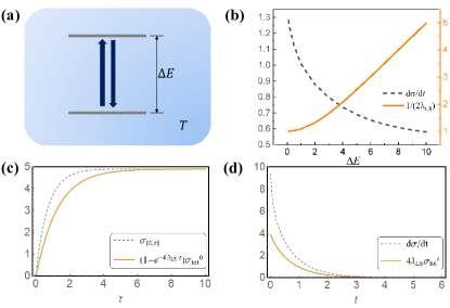
Figure 1: Illustration of the trade-off relation and the lower bound for entropy production in a two-state mode. Here, we set $\beta=1/(k_{B}T)=1$. (a) The two-state model coupled to a heat reservoir with temperature $T$. (b) The trade-off relation between the entropy production rate $\dot{\sigma}(t)$ at $t=0$ and the relaxation time scale $1/(2\lambda_{\text{LS}})$ for relaxation processes with different $\Delta E$, where the distance to equilibrium $\sigma_{\text{tot}}^{t}$ is fixed to be $0.5$. (c) and (d) We demonstrate Eq. (10) and (11) for this model, in which $\Delta E=5.0$ and the initial distribution is chosen to be $(p_{u},p_{d})=(0.99,0.01)$.

It should be noted that, the lower bound for entropy production rate (or trade-off relation) we find is not limited to the discrete-state systems and classical systems. Thanks to the fact that the entropy production still has a close connection with the KL divergence in open quantum systems Breuer et al. (2002) and continuous-space Markovian systems Van den Broeck and Esposito (2010), similar lower bounds can be found in both of the systems, as shown in Sec. IV of SM.

Inverse speed limit.— A direct corollary of Eq. (10) is an inverse speed limit:

$$\tau \leq\frac{1}{4\lambda_{\text{LS}}}\ln\left\{\frac{\sigma_{\text{tot}}^{0}}{\sigma_{\text{tot}}^{0}-\sigma_{[0,\tau]}}\right\}$$

$$\leq\frac{\tau_{\text{rel}}}{2}\ln\left\{\frac{\sigma_{\text{tot}}^{0}}{\sigma_{\text{tot}}^{0}-\sigma_{[0,\tau]}}\right\},$$ (15)

which gives the upper bound for the time $\tau$ of the relaxation from an initial distribution $\boldsymbol{p}(0)$ to a target distribution $\boldsymbol{p}(\tau)$. The inverse speed limit in relaxation processes is our another main result. Crucially, this bound holds for any $\tau$, in contrast to the time-scale estimation $1/\lambda_{g}$ from the spectral gap $\lambda_{g}$, which only works in the large time limit. A physical interpretation of this bound is that when the entropy production cost $\sigma_{[0,\tau]}$ for the state transformation from $\boldsymbol{p}(0)$ to $\boldsymbol{p}(\tau)$ is fixed, a large initial thermodynamic cost $\sigma_{\text{tot}}(0)$ is needed to make the transformation time $\tau$ in relaxation shorter. In other words, to ensure faster relaxation, a large amount of energy should be cost to drive the system farther from equilibrium. Indeed, Eq. (15) tells that once the system is initially far enough from equilibrium, i.e., the $\sigma_{\text{tot}}(0)$ is large enough, the relaxation time can be very short even when the target state $\boldsymbol{p}(\tau)$ is rather far from the initial state. Remarkably, our upper bound provides a experimentally accessible strategy to estimate the transformation time $\tau$, since the relaxation time $\tau_{\text{rel}}$ can be approximately replaced by the experimentally measured relaxation time scale. Thus, our bound solely consists of directly measurable quantities and may be utilized in actual experiments without knowing any dynamical details. Together with the result from N. Shiraishi and K. Saito Shiraishi and Saito (2019), one can bound the transformation time $\tau$ both from above and below:

$$\frac{D[\boldsymbol{p}(0)||\boldsymbol{p}(\tau)]}{\bar{\sigma}_{[0,\tau]}}\leq\tau\leq\frac{1}{4\lambda_{\text{LS}}}\ln\left\{\frac{\sigma_{\text{tot}}^{0}}{\sigma_{\text{tot}}^{0}-\sigma_{[0,\tau]}}\right\},$$ (16)

where $\bar{\sigma}_{[0,\tau]}=\text{$\sigma_{[0,\tau]}$}/\tau$ is the average entropy production rate during transformation. The two bounds better characterizes the time transforming from a given state to another in thermal relaxation.

In addition, note that our upper bound still works when the detailed balance condition is not satisfied, the only difference is that the entropy production should be replaced with the non-adiabatic entropy production $\sigma^{\text{na}}$ and a factor $1/2$ should be multiplied to the right:

$$\tau \leq\frac{1}{2\lambda_{\text{LS}}}\ln\left\{\frac{\sigma_{\text{tot}}^{0,\text{na}}}{\sigma_{\text{tot}}^{0,\text{na}}-\sigma_{[0,\tau]}^{\text{na}}}\right\}$$

$$\leq\tau_{\text{rel}}\ln\left\{\frac{\sigma_{\text{tot}}^{0,\text{na}}}{\sigma_{\text{tot}}^{0,\text{na}}-\sigma_{[0,\tau]}^{\text{na}}}\right\}.$$ (17)

The total entropy production can be decomposed as $\sigma_{[0,\tau]}=\sigma_{[0,\tau]}^{\text{na}}+\sigma_{[0,\tau]}^{\text{hs}}$, where $\sigma_{[0,\tau]}^{\text{hs}}$ is the housekeeping entropy production cost for maintaining nonequilibrum stationary states Seifert (2012). Therefore, the above result (17) for the relaxation to nonequilibrium stationary states implies that only the non-adiabatic entropy production is crucial, and the stationary (housekeeping) entropy production rate may play no roles in time-scale of thermal relaxation processes.

It is worth mentioning that, one can obtain other upper bounds of the transformation time $\tau$ simply by replacing the KL divergence with other distance functions, though the physical meaning of which may be not that clear. For instance, if one choose the $L_{2}$ norm (the definition is $||f||_{2}\equiv\sqrt{\langle f,f\rangle_{\pi}}$) as the distance function, a different upper bound for $\tau$ can be derived as

$$\tau\leq\frac{1}{\lambda_{g}}\ln\frac{||\boldsymbol{p}(\tau)-\boldsymbol{p}^{\text{eq}}||_{2}}{||\boldsymbol{p}(0)-\boldsymbol{p}^{\text{eq}}||_{2}},$$ (18)

with the spectral gap $\lambda_{g}$ being defined as

$$\lambda_{g}=\inf_{\langle f,f\rangle_{\pi}\neq 0}\frac{\text{Re}\langle-\mathcal{\mathcal{L}}f,f\rangle_{\pi}}{\langle f,f\rangle_{\pi}}.$$ (19)

Which upper bound is tighter remains to be explored. Further, there even may exist one kind of distance function that can optimize the estimation of $\tau$, i.e., make the upper bound tightest, which we leave for future study.

Sketch of the proof of Eq. (3).—To prove Eq. (3), it is equivalently to prove

$$\frac{\text{d}}{\text{d}t}D[\boldsymbol{p}(t)||\boldsymbol{\pi}_{t}]-\dot{\boldsymbol{\pi}}_{t}\partial_{\boldsymbol{\pi}_{t}}D[\boldsymbol{p}(t)||\boldsymbol{\pi}_{t}]\leq-4\lambda_{\text{LS}}(t)D[\boldsymbol{p}(t)||\boldsymbol{\pi}_{t}].$$ (20)

Note $\frac{\text{d}}{\text{d}\tau}D[\boldsymbol{p}(\tau)||\boldsymbol{\pi}_{t}]|_{\tau=t}$ equals to the left hand side, which can then be directly computed as

$$\frac{\text{d}}{\text{d}\tau}D[\boldsymbol{p}(\tau)||\boldsymbol{\pi}_{t}]|_{\tau=t}= \dot{\boldsymbol{p}}\partial_{\boldsymbol{p}}D[\boldsymbol{p}||\boldsymbol{\pi}_{t}]$$

$$= \sum_{i}\dot{p}_{i}(t)\left[\ln\frac{p_{i}(t)}{\pi_{i}^{t}}+1\right]$$

$$= \sum_{i}\mathcal{L}(t)p_{i}(t)\ln\frac{p_{i}(t)}{\pi_{i,t}}$$

$$= -\langle\ln\frac{\boldsymbol{p}(t)}{\boldsymbol{\pi}_{t}},-\mathcal{L}\left(\frac{\boldsymbol{p}(t)}{\boldsymbol{\pi}_{t}}\right)\rangle_{\pi},$$ (21)

where in the first and third line, the relation $\dot{D}[\boldsymbol{p}||\boldsymbol{\pi}_{t}]=\dot{\boldsymbol{p}}\partial_{\boldsymbol{p}}D[\boldsymbol{p}||\boldsymbol{\pi}_{t}]+\dot{\boldsymbol{\pi}}_{t}\partial_{\boldsymbol{\pi}_{t}}D[\boldsymbol{p}||\boldsymbol{\pi}_{t}]$ and the conservation of probability $\frac{\text{d}}{\text{d}t}\sum_{i}p_{i}(t)=0$ have been used. Defining $f(t)\equiv\frac{\boldsymbol{p}(t)}{\boldsymbol{\pi}_{t}}$, it can be shown that with detailed balance condition (see SM for details and the case without detailed balance condition),

$$-\langle\ln f,-\mathcal{L}f\rangle_{\pi}(t)\leq- 4\text{Re}\langle-\mathcal{L}\sqrt{f},\sqrt{f}\rangle_{\pi}(t)$$

$$\leq- 4\lambda_{\text{SL}}(t)\text{Ent}(\sqrt{f})(t)$$

$$=- 4\lambda_{\text{SL}}\sum_{i=1}^{N}\frac{p_{i}(t)}{\pi_{i}^{t}}\ln\left(\frac{p_{i}(t)}{\pi_{i}^{t}}\right)\pi_{i}^{t}$$

$$=- 4\lambda_{\text{SL}}(t)D[\boldsymbol{p}(t)||\boldsymbol{\pi}_{t}],$$ (22)

which leads to the desired inequality (20). In the second last line, the identity $\langle\sqrt{\frac{\boldsymbol{p}(t)}{\boldsymbol{\pi}_{t}}},\sqrt{\frac{\boldsymbol{p}(t)}{\boldsymbol{\pi}_{t}}}\rangle_{\pi}=1$ has been used. And note that when $f=\boldsymbol{p}(t)/\boldsymbol{\pi}$, one has $\text{Ent}(\sqrt{f})=D[\boldsymbol{p}(t)||\boldsymbol{\pi}]$.

Discussion.— In this letter, we propose a general lower bound for entropy production related to the LS constant and KL divergence and utilize it to find a trade-off relation that deepens the understanding of thermal relaxation processes. The trade-off relation may be utilized to experimentally estimate entropy production irrespective of model details in that we believe one can safely approximate the LS constant using relaxation time to stationarity observed in actual experiments, i.e., $\dot{\sigma}(t)\tau_{\text{rel}}\geq 2\sigma_{\text{tot}}^{t}$. Another important consequence of the bound is an inverse speed limit for transforming states in thermal relaxation, which can improve the estimation of the transformation time. The inverse speed limit is pertinent to the thermodynamic cost in thermal relaxation, which may be used to optimize relaxation processes. Additionally, it may uncover that a system is unlikely to be trapped in a metastable state for more time than a certain threshold.

To summarize, this letter reveals some hidden general properties of thermal relaxation dynamics and paves the way for further application of LS constant in stochastic thermodynamics. However, the complete information of the dynamics is contained in all eigenvalues of the stochastic matrix. It is thus still an open problem to analyze thermal relaxation processes beyond the spectral gap and LS constant, which only characterize the slowest dynamical mode.

We are grateful to Guangyi Zou, Zhiyu Cao and Shiling Liang for useful discussions. This work is supported by MOST(2022YFA1303100), NSFC (32090044).

Supplemental Material for “A Universal Trade-off Relation Between Dissipation and Relaxation Time-scale and An Inverse Speed Limit in Thermal Relaxation”

Appendix A Detailed derivation of Eq. (3) in the main text

Without loss of generality, we assume transition rates $k_{ij}$ satisfy the normalization condition $\sum_{i}k_{ij}=1$ throughout this section. Releasing the constraint, the only difference is a multiplicative factor $\sum_{i}k_{ij}$, which will not affect the derivations here. Under the condition, the stochastic matrix $\mathcal{L}(t)$ in the main text can be written as $K(t)-\mathbb{I}$, where $K_{ij}(t)=k_{ij}(t)$ and $\mathbb{I}$ is the identity matrix. Then for any function $f$, the operator $K$ satisfies $(Kf)_{i}=\sum_{j}k_{ij}f_{j}$. Recall that the the inner product induced by the stationary distribution is defined as

$$\langle f,g\rangle_{\pi}=\sum_{i}f_{i}g_{i}^{\dagger}\pi_{i}.$$ (23)

Based on this inner product, one can further define an adjoint operator $\mathcal{L}^{\star}$ of $\mathcal{L}$ as $\langle f,\mathcal{L}g\rangle_{\pi}=\langle\mathcal{L}^{\star}f,g\rangle_{\pi}$ for any function $f$ and $g$. Likewise, another adjoint operator $K^{\star}$ of $K$ is given by $\langle f,Kg\rangle_{\pi}=\langle K^{\star}f,g\rangle_{\pi}$. Consequently, one can readily check that the operator $K^{\star}$ satisfies $(K^{\star}f)_{j}=\sum_{i}k_{ij}f_{i}$. These relations will be useful in the derivations below. For more details, see Ref. Diaconis and Saloff-Coste (1996). Moreover, one can define the LS constant with respect to $\mathcal{L}_{s}\equiv(\mathcal{L}+\mathcal{L}^{\star})/2$, the symmetrized version of $\mathcal{L},$ as

$$\lambda_{\text{LS}}= \inf_{\text{Ent}(f)\neq 0}\frac{\text{Re}\langle-\mathcal{L}f,f\rangle_{\pi}}{\text{Ent}(f)}$$

$$= \inf_{\text{Ent}(f)\neq 0}\frac{\langle-\mathcal{L}_{s}f,f\rangle_{\pi}}{\text{Ent}(f)}.$$ (24)

Note that $\mathcal{L}^{\star}=\mathcal{L}$ so that $\mathcal{L}_{s}=\mathcal{L}$ when the detailed balance condition holds. We drop $t$ dependence in the following for notation’s brevity.

Lemma 1: $$\text{Re}\langle-\mathcal{L}^{\star}f,f\rangle_{\pi}=\frac{1}{2}\sum_{i,j}|f_{i}-f_{j}|^{2}k_{ij}\pi_{j},$$ (25)

where $|A|\equiv\sqrt{AA^{\dagger}}$.

Proof:

Notice that $\text{Re}\langle-\mathcal{L}^{\star}f,f\rangle_{\pi}=\text{Re}\langle(\mathbb{I}-K^{\star})f,f\rangle_{\pi}=\langle f,f\rangle_{\pi}-\text{Re}\langle K^{\star}f,f\rangle_{\pi}$, and the right hand side of Eq. (25) can be rewritten as

$$\frac{1}{2}\sum_{i,j}|f_{i}-f_{j}|^{2}k_{ij}\pi_{j}= \frac{1}{2}\sum_{i,j}\left[|f_{i}|^{2}+|f_{j}|^{2}-2\text{Re}(f_{i}f_{j}^{\dagger})\right]k_{ij}\pi_{j}$$ (26)

$$= \frac{\sum_{i}|f_{i}|^{2}\sum_{j}k_{ij}\pi_{j}+\sum_{j}|f_{j}|^{2}\pi_{j}\sum_{i}k_{ij}}{2}-\text{Re}\sum_{i,j}k_{ij}f_{i}f_{j}^{\dagger}\pi_{j}$$ (27)

$$= \frac{\sum_{i}|f_{i}|^{2}\pi_{i}+\sum_{j}|f_{j}|^{2}\pi_{j}}{2}-\text{Re}\sum_{j}(K^{\star}f)_{j}f_{j}^{\dagger}\pi_{j}$$ (28)

$$= \langle f,f\rangle_{\pi}-\text{Re}\langle K^{\star}f,f\rangle_{\pi},$$ (29)

where in the third line, the identities $\sum_{j}k_{ij}\pi_{j}=\pi_{i}$ and $\sum_{i}k_{ij}=1$ have been used. Therefore, $\text{Re}\langle-\mathcal{L}^{\star}f,f\rangle_{\pi}=\langle f,f\rangle_{\pi}-\text{Re}\langle K^{\star}f,f\rangle_{\pi}=\frac{1}{2}\sum_{i,j}|f_{i}-f_{j}|^{2}k_{ij}\pi_{j}$.

Further, with the detailed balance condition $k_{ij}\pi_{j}=k_{ji}\pi_{i}$ holding, one can similarly show that

$$\text{Re}\langle-\mathcal{L}f,g\rangle_{\pi}=\frac{1}{2}\sum_{i,j}\left(f_{i}-f_{j}\right)\left(g_{i}-g_{j}\right)k_{ij}\pi_{j}.$$ (30)

Note that $f$ can be a complex function and $f_{i}^{\dagger}$ denote the complex conjugate of $f_{i}$.

Lemma 2:

For a system with detailed balance condition ($\boldsymbol{\pi}=\boldsymbol{p}^{\text{eq}}$), any function $f$ in the state space of the system satisfies:

$$\langle-\mathcal{L}^{\star}\ln f,f\rangle_{\pi}\geq 4\langle-\mathcal{L}^{\star}\sqrt{f},\sqrt{f}\rangle_{\pi}.$$ (31)

Additionally, in the absence of detailed balance condition, a weaker inequality

$$\langle-\mathcal{L}^{\star}\ln f,f\rangle_{\pi}\geq 2\langle-\mathcal{L}^{\star}\sqrt{f},\sqrt{f}\rangle_{\pi}$$ (32)

holds.

Proof:

For any $a,b>0$,

$$\left(\frac{\sqrt{a}-\sqrt{b}}{a-b}\right)^{2}= \left[\frac{1}{2(a-b)}\int_{b}^{a}x^{-\frac{1}{2}}\text{d}x\right]^{2}$$

$$\leq \left[\int_{b}^{a}\frac{1}{4(a-b)^{2}}\text{d}x\right]\left(\int_{b}^{a}x^{-1}\text{d}x\right)=\frac{1}{4}\frac{\ln a-\ln b}{a-b}$$ (33)

thus the inequality below is fulfilled:

$$\left(a-b\right)\left[\ln a-\ln b\right] \geq 4\left(\sqrt{a}-\sqrt{b}\right)^{2}.$$ (34)

Then using Lemma 1 and Eq. (30), the inequality $\langle-\mathcal{L}^{\star}\ln f,f\rangle_{\pi}\geq 4\langle-\mathcal{L}^{\star}\sqrt{f},\sqrt{f}\rangle_{\pi}$ is immediately derived. For any $a,b>0$, there is another inequality

$$\ln a^{2}-\ln b^{2}\leq\frac{2(a-b)}{b}$$ (35)

due to the concavity of the function $\ln x^{2}$. Multiplying both sides by $b^{2}$ leads to

$$b^{2}(\ln a^{2}-\ln b^{2})\leq 2b(a-b).$$ (36)

Then let $f_{i}=b^{2}$ and $(K\ln f)_{i}=\ln a^{2}$, one obtains

$$f_{i}[(K^{\star}-\mathbb{I})\ln f]_{i}\leq 2\sqrt{f_{i}}(\sqrt{e^{K^{\star}\ln f}}-\sqrt{f})_{i}\leq 2\sqrt{f_{i}}[(K^{\star}-\mathbb{I})\sqrt{f}]_{i},$$ (37)

where the inequality

$$(\sqrt{e^{K^{\star}\ln f}})_{i}=\sqrt{e^{\sum_{j}k_{ji}(\ln f)_{j}}} \leq \sum_{j}k_{ji}(\sqrt{e^{\ln f_{j}}})=K^{\star}\sqrt{f}$$

has been used (the inequality is from the convexity of the function $\sqrt{e^{x}}$ and the Jensen inequality). Notice that $-\mathcal{L}^{\star}=\mathbb{I}-K^{\star}$, thus Eq. (37) is equal to

$$[(-\mathcal{L}^{\star})\ln f]_{i}f_{i}\pi_{i}\geq 2[(-\mathcal{L}^{\star})\sqrt{f}]_{i}\sqrt{f_{i}}\pi_{i},$$ (38)

which directly yields $\langle-\mathcal{L}^{\star}\ln f,f\rangle_{\pi}\geq 2\langle-\mathcal{L}^{\star}\sqrt{f},\sqrt{f}\rangle_{\pi}$.

Proof of the Eq. (3) in the main text:

Equipped with Lemma 1 and Lemma 2, we can prove the inequality (3) (with detailed balance) as follow:

$$\frac{\text{d}}{\text{d}t}D[\boldsymbol{p}(t)||\boldsymbol{\pi}_{\tau}]|_{\tau=t}= \sum_{i}[1+\ln\frac{p_{i}(t)}{\pi_{i}^{t}}]\dot{p}_{i}(t)$$ (39)

$$= \sum_{i}\ln\frac{p_{i}(t)}{\pi_{i}^{t}}\frac{\text{d}}{\text{d}t}\left[\frac{p_{i}(t)}{\pi_{i}^{t}}\right]\pi_{i}$$ (40)

$$= -\sum_{i}\ln\frac{p_{i}(t)}{\pi_{i}^{t}}\left[-\mathcal{L}\frac{\boldsymbol{p}(t)}{\boldsymbol{\pi}_{t}}\right]_{i}\pi_{i}$$ (41)

$$= -\langle\ln\frac{\boldsymbol{p}(t)}{\boldsymbol{\pi}_{t}},-\mathcal{L}\frac{\boldsymbol{p}(t)}{\boldsymbol{\pi}_{t}}\rangle_{\pi}$$ (42)

$$\equiv -\langle\ln f(t),-\mathcal{L}f(t)\rangle_{\pi}$$ (43)

$$= -\langle-\mathcal{L}^{\star}\ln f(t),f(t)\rangle_{\pi}$$ (44)

$$\leq -4\langle-\mathcal{L}^{\star}\sqrt{f(t)},\sqrt{f(t)}\rangle_{\pi}$$ (45)

$$= -4\text{Re}\langle-\mathcal{L}\sqrt{f(t)},\sqrt{f(t)}\rangle_{\pi}\leq-4\lambda_{\text{LS}}(t)\text{Ent}(\sqrt{f(t)})$$ (46)

$$= -4\lambda_{\text{LS}}(t)\sum_{i=1}^{N}|\sqrt{\frac{p_{i}(t)}{\pi_{i}^{t}}}|^{2}\ln\left(\frac{|\sqrt{\frac{p_{i}(t)}{\pi_{i}}}|^{2}}{\langle\sqrt{\frac{\boldsymbol{p}(t)}{\boldsymbol{\pi}_{t}}},\sqrt{\frac{\boldsymbol{p}(t)}{\boldsymbol{\pi}_{t}}}\rangle_{\pi}}\right)\pi_{i}^{t}$$ (47)

$$= -4\lambda_{\text{LS}}(t)D[\boldsymbol{p}(t)||\boldsymbol{\pi}_{t}].$$ (48)

It should be noted that, since $f(t)=\frac{\boldsymbol{p}(t)}{\boldsymbol{\pi}_{t}}$ is a real function and $\langle-\mathcal{L}^{\star}f,f\rangle_{\pi}=\langle f,-\mathcal{L}f\rangle_{\pi}=\langle-\mathcal{L}f,f\rangle_{\pi}^{\dagger}$, we get that $\langle-\mathcal{L}^{\star}f,f\rangle_{\pi}=\text{Re}\langle-\mathcal{L}^{\star}f,f\rangle_{\pi}=\text{Re}\langle-\mathcal{L}f,f\rangle_{\pi}$, which has been used in the third last line. Without detailed balance, Eq. (45) should be substituted with $-2\langle-\mathcal{L}^{\star}\sqrt{f(t)},\sqrt{f(t)}\rangle_{\pi}$, where the only difference is a multiplicative constant $1/2$.

The discussions above can be naturally generalized to the system coupled to multiple heat baths, in which the stochastic matrix consists of contributions from each independent baths as $\mathcal{L}(t)=\sum_{\nu}\mathcal{L}^{\nu}(t)$, with $\mathcal{L}^{\nu}(t)$ being the stochastic matrix related to the $\nu$th bath. With multiple heat baths, the non-adiabatic entropy production rate can still be associated with the KL divergence as

$$\dot{\sigma}^{\text{na}}(t)=-\sum_{i}\dot{p}_{i}(t)\ln\frac{p_{i}(t)}{\pi_{i}^{t}}=-\frac{\text{d}}{\text{d}t}D[\boldsymbol{p}(t)||\boldsymbol{\pi}_{\tau}]|_{\tau=t}.$$ (49)

Notably, $\dot{\sigma}^{\text{na}}(t)$ is only a function of the coarse-grained transition rates $k_{ij}(t)=\sum_{\nu}k_{ij}^{\nu}(t)$, which is not pertinent to the individual contribution from the $\nu$th heat bath. Therefore, the general bound (6) in the main text can be directly generalized to the system coupled to multiple heat baths as

$$\dot{\sigma}(t)\geq\dot{\sigma}^{\text{na}}(t)\geq 2\lambda_{\text{LS}}(t)D[\boldsymbol{p}(t)||\boldsymbol{\pi}_{t}].$$ (50)

As mentioned in the main text, the total entropy production rate can be decomposed into two parts, one part is the non-adiabatic entropy production, and another part (housekeeping or adiabatic entropy production rate) reads

$$\dot{\sigma}^{\text{hs}}(t)=\sum_{\nu}\sum_{i,j}k_{ij}^{\nu}(t)p_{j}(t)\ln\frac{k_{ij}^{\nu}(t)\pi_{j}^{t}}{k_{ji}^{\nu}(t)\pi_{i}^{t}}.$$ (51)

It can be seen from this expression that only if the transitions induced by every heat bath all satisfy the detailed balance condition, i.e., $k_{ij}^{\nu}(t)\pi_{j}^{t}=k_{ji}^{\nu}(t)\pi_{i}^{t}$ for any $\nu$, will the housekeeping part vanish (so that $\boldsymbol{\pi}_{t}=\boldsymbol{p}_{t}^{\text{eq}}$). In this case, $\dot{\sigma}(t)=\dot{\sigma}^{\text{na}}(t)\geq 4\lambda_{\text{LS}}(t)D[\boldsymbol{p}(t)||\boldsymbol{p}_{t}^{\text{eq}}]$.

Appendix B An application of Eq. (6) to time-dependent dynamics

In this section, we are interested in an example considered in Refs. Busiello et al. (2021b); Zhang et al. (2023), where the transition matrix is under periodic oscillations. This setting has actual applications in biological and chemical systems. As a result, the dynamics is governed by a time-dependent stochastic matrix : $\frac{\text{d}}{\text{d}t}\boldsymbol{p}(t)=\mathcal{L}(t)\boldsymbol{p}(t),$ where

$$\mathcal{L}(t)=\begin{cases}\mathcal{L}_{1}&t\in[2n\tau,(2n+1)\tau]\\ \mathcal{L}_{2}&t\in[(2n+1)\tau,(2n+2)\tau]\end{cases},\ n\in\mathbb{N}.$$ (52)

Here, $\mathcal{L}_{1}$ and $\mathcal{L}_{2}$ are time-independent stochastic matrices satisfying the detailed balance condition and $\tau$ is the period of oscillation. The LS constant of $\mathcal{L}_{1}$ and $\mathcal{L}_{2}$ are denoted as $\lambda_{\text{LS,1}}$ and $\lambda_{\text{LS,2}}$ respectively. The system under this setting will finally converge to a periodic stationary state in which $\boldsymbol{p}(t)=\boldsymbol{p}(t+\tau)$.

In the fast oscillation limit $\tau\rightarrow 0$, it has been demonstrated that the periodic stationary state reduces to an effective equilibrium state $\boldsymbol{p}^{\text{eff}}$ corresponding to an effective stochastic matrix

$$\mathcal{L}^{\text{eff}}\equiv\frac{\mathcal{L}_{1}+\mathcal{L}_{2}}{2},$$ (53)

i.e.,

$$\mathcal{L}^{\text{eff}}\boldsymbol{p}^{\text{eff}}=0.$$ (54)

The effective LS constant corresponding to the effective stochastic matrix is given by

$$\lambda_{\text{LS}}^{\text{eff}}= \inf_{\text{Ent}(f)\neq 0}\frac{\text{Re}\langle-\mathcal{\mathcal{L}^{\text{eff}}}f,f\rangle_{\pi}}{\text{Ent}(f)}$$

$$= \frac{1}{2}\inf_{\text{Ent}(f)\neq 0}\frac{\text{Re}\langle-\left(\mathcal{L}_{1}+\mathcal{L}_{2}\right)f,f\rangle_{\pi}}{\text{Ent}(f)}$$

$$= \frac{\inf_{\text{Ent}(f)\neq 0}\frac{\text{Re}\langle-\mathcal{L}_{1}f,f\rangle_{\pi}}{\text{Ent}(f)}+\inf_{\text{Ent}(f)\neq 0}\frac{\text{Re}\langle-\mathcal{L}_{2}f,f\rangle_{\pi}}{\text{Ent}(f)}}{2}$$

$$= \frac{\lambda_{\text{LS,1}}+\lambda_{\text{LS,2}}}{2}.$$ (55)

Then, applying our first main result Eq. (7) to the situation when the system has reached the effective equilibrium yields that

$$\text{$\dot{\sigma}(t)$}\geq 2\left(\lambda_{\text{LS,1}}+\lambda_{\text{LS,2}}\right)D\left[\boldsymbol{p}^{\text{eff}}||\boldsymbol{p}_{t}^{\text{eq}}\right],$$ (56)

since the system is in the effective equilibrium state and the effective LS constant is given by $(\lambda_{\text{LS,1}}+\lambda_{\text{LS,2}})/2$. Note that the instantaneous equilibrium distribution $\boldsymbol{p}_{t}^{\text{eq}}$ at time $t$ will be one of the equilibrium distributions $\boldsymbol{p}_{1}^{\text{eq}}$ or $\boldsymbol{p}_{2}^{\text{eq}}$ corresponding to $\mathcal{L}_{1}$ or $\mathcal{L}_{2}$, which are not matched with the effective equilibrium state. As a consequence, $D\left[\boldsymbol{p}^{\text{eff}}||\boldsymbol{p}_{t}^{\text{eq}}\right]>0$ so that the lower bound given by Eq. (56) is positive. For a very large time $t\gg\tau$, one can further bound the entropy production $\sigma_{[0,t]}$ during the interval $[0,t]$ asymptotically from below as

$$\sigma_{[0,t]}\gtrsim\left(\lambda_{\text{LS,1}}+\lambda_{\text{LS,2}}\right)\left(D\left[\boldsymbol{p}^{\text{eff}}||\boldsymbol{p}_{1}^{\text{eq}}\right]+D\left[\boldsymbol{p}^{\text{eff}}||\boldsymbol{p}_{2}^{\text{eq}}\right]\right)t$$ (57)

This is remarkable because the system in an effective equilibrium state may not be distinguished from a real equilibrium state in a coarse grained level, e.g., in the experimental observations level, which may lead to the wrong conclusion that there is no entropy production. However, our positive bound can recover at least part of the “hidden” entropy production (rate), which is notably stronger than the conventional second law of thermodynamics. We should emphasize that even when the system is not periodically switching, but randomly switching between two configurations $\mathcal{L}_{1}$ and $\mathcal{L}_{2}$ at a constant Poisson rate $r$, the above result can still apply in the fast switching limit $r\rightarrow\infty$, when the system is still in an effective equilibrium state corresponding to $\mathcal{L}^{\text{eff}}$.

Certainly, our bound is not limited to the fast oscillation limit, when the period $\tau$ is finite, our lower bound can still be applied and probably give a positive value. For example, assuming $t>\tau$ and $\mathcal{L}(0)=\mathcal{L}_{1}$, one can utilize obtain a positive lower bound for $\sigma_{[0,t]}$ in this case, as

$$\sigma_{[0,t]}\geq\left[1-e^{-4\lambda_{\text{LS,1}}\tau}\right]D\left[\boldsymbol{p}(0)||\boldsymbol{p}_{\mathcal{L}_{1}}^{\text{eq}}\right]+\left[1-e^{-4\lambda_{\text{LS,2}}(t-\tau)}\right]D\left[\boldsymbol{p}(\tau)||\boldsymbol{p}_{\mathcal{L}_{2}}^{\text{eq}}\right],$$ (58)

where $\boldsymbol{p}(\tau)=\mathcal{T}e^{\int_{0}^{\tau}\mathcal{L}_{1}\text{d}t}\boldsymbol{p}(0)$, $\mathcal{T}$ is the time-ordering.

Appendix C Properties of the LS constant and its relation to the spectral gap

The LS constant characterizes the relaxation timescale as

$$\frac{1}{2\lambda_{\text{LS}}}\leq\tau_{\text{rel}}\leq\frac{4+\log\log[1/\pi_{\star}]}{2\lambda_{\text{LS}}},$$

where $\pi_{\star}\equiv\min_{i}\pi_{i}$ and the relaxation time $\tau_{\text{rel}}$ is defined as

$$\tau_{\text{rel}}=\inf\left\{t>0:\sup_{i}\left\|\frac{\boldsymbol{p}(t|p_{j}(0)=\delta_{ij})}{\boldsymbol{\pi}}-\mathbb{I}\right\|_{2}\leq\frac{1}{e}\right\},$$

with the $L_{2}$ norm being defined as $||f||_{2}\equiv\sqrt{\langle f,f\rangle_{\pi}}=\sqrt{\sum_{i}|f_{i}|^{2}\pi_{i}}$ and $\mathbb{I}$ being the identity matrix. When the unique stationary distribution $\boldsymbol{\pi}$ is an equilibrium distribution $\boldsymbol{p}^{\text{eq}}$, the upper bound of $\tau_{\text{rel}}$ can be enhanced by a factor $1/2$. There are similar inequalities for $\tau_{\text{rel}}$ using the spectral gap $\lambda_{g}$ when detailed balance condition holds, i.e.,

$$\frac{1}{\lambda_{g}}\leq\tau_{\text{rel}}\leq\frac{2+\log[1/\pi_{\star}]}{2\lambda_{g}}.$$

Further, there is a hierarchical relation between the spectral gap $\lambda_{g}$ and LS constant $\lambda_{\text{LS}}$ Giné et al. (2006):

$$\frac{\lambda_{g}}{2}\geq\lambda_{\text{LS}}\geq\frac{1-2\pi_{\star}}{\ln(1-\pi_{\star}/\pi_{\star})}\lambda_{g}>0.$$ (59)

The spectral gap $\lambda_{g}$ is the second largest eigenvalue of $-\mathcal{L}_{s}$, and it has a similar definition to $\lambda_{\text{LS}}$ as

$$\lambda_{g}= \inf_{\langle f,f\rangle_{\pi}\neq 0}\frac{\text{Re}\langle-\mathcal{\mathcal{L}}f,f\rangle_{\pi}}{\langle f,f\rangle_{\pi}}$$

$$= \inf_{\langle f,f\rangle_{\pi}\neq 0}\frac{\langle-\mathcal{\mathcal{L}}_{s}f,f\rangle_{\pi}}{\langle f,f\rangle_{\pi}}.$$ (60)

Note that when the detailed balance condition holds, $\mathcal{\mathcal{L}}_{s}=\mathcal{\mathcal{L}}$ so that $\lambda_{g}$ becomes the second largest eigenvalue of $-\mathcal{L}$ in this case.

Consequently, $\lambda_{\text{LS}}$ may characterize the relaxation timescale better compared with the spectral gap $\lambda_{g}$ due to the hierarchical relation above (the inequality from $\lambda_{\text{LS}}$ is tighter than the inequality from $\lambda_{g}$).

Due to the close connection between $\lambda_{\text{LS}}$ and the spectral gap $\lambda_{g}$ which is usually easier to determined, one can obtain another useful bound related to $\lambda_{g}$ as

$$\dot{\sigma}(t)\geq 4C\lambda_{g}\sigma_{\text{tot}}^{t},$$ (61)

where $C=(1-2\pi_{\star})/\ln(1-\pi_{\star}/\pi_{\star})$. This bound uncovers a connection between the thermodynamic irreversibility and the spectrum of the dynamical generator in thermal relaxation.

Appendix D Generalization to open quantum systems and continuous-space Markov processes

D.1 Generalization to Markovian open quantum systems

Here we show that, our main results can be generalized to quantum Markov processes described by the Lindblad master equations. In this setting, the dynamics of the density operator $\rho_{t}\equiv\rho(t)$ at time $t$ is given by $\dot{\rho}_{t}=\mathcal{L}(\rho_{t}),$ where

$$\mathcal{L}(\rho)\equiv-i[H,\rho]+\sum_{i}\left[J_{i}\rho J_{i}^{\dagger}-\frac{1}{2}\{J_{i}^{\dagger}J_{i},\rho\}\right]$$ (62)

is the Lindbladian. Here, $H$ is the Hamiltonian in a $d-$dimensional Hilbert space $\mathcal{H}^{d}$ and $J_{i}$ is the $j$th jump operator describing dissipation effect due to the environment. To proceed, we assume that the Lindbladian satisfies the quantum detailed balance condition Firanko et al. (2022), in which case the density operator will finally converge to a Gibbs state $\rho_{\beta}=\lim_{t\rightarrow\infty}e^{\mathcal{L}t}\rho_{0}=e^{-\beta H}/\text{Tr($e^{-\beta H}$)}$. The inner product should be redefined as $\langle A,B\rangle_{\pi}\equiv\text{Tr}(A^{\dagger}B\rho_{\beta})$, the average over the Gibbs state reads $\langle A\rangle_{\pi}\equiv\text{Tr}(A\rho_{\beta})$ and the quantum KL divergence is given by $D(\rho||\rho^{\prime})=\text{Tr}(\rho\ln\rho-\rho\ln\rho^{\prime})$. The entropy production rate $\dot{\sigma}_{t}$ at time $t$ in the open quantum systems can be separated to the change rate of system entropy $\dot{s}_{t}=\text{Tr}(\dot{\rho_{t}}\ln\rho_{t})$ and the heat flow $\beta\dot{q}=\beta\text{Tr($\dot{\rho}_{t}H$)}$ as $\dot{\sigma}_{t}=\dot{s}_{t}-\beta\dot{q}$. Like in the classical case, $\dot{\sigma}_{t}$ has a direct connection with KL divergence that $\dot{\sigma}_{t}=-\partial_{t}D(\rho_{t}||\rho_{\beta})$ Breuer et al. (2002). Recently, it has been proved that there always exist a positive constant $\alpha$ assuring that the quantum LS inequality

$$-\langle\mathcal{L}(f),\ln f\rangle_{\pi}\geq\alpha\langle f\ln f\rangle_{\pi}$$ (63)

holds Gao and Rouzé (2022) for any postive operator $f\in\mathcal{H}^{d}$ satifying $\langle f\rangle_{\pi}=1$, once the quantum detailed balance condition is satisfied. Consequently, a straightforward calculation shows that,

$$\dot{\sigma}_{t}= -\partial_{t}D(\rho_{t}||\rho_{\beta})$$

$$= -\langle\mathcal{L}(\frac{\rho_{t}}{\rho_{\beta}}),\ln\frac{\rho_{t}}{\rho_{\beta}}\rangle_{\pi}$$

$$\geq \lambda_{\text{QLS}}\langle\frac{\rho_{t}}{\rho_{\beta}}\ln\frac{\rho_{t}}{\rho_{\beta}}\rangle_{\pi},$$

$$= \lambda_{\text{QLS}}D(\rho_{t}||\rho_{\beta}),$$ (64)

where

$$\lambda_{\text{QLS}}\equiv\inf_{f>0,\ \langle f\rangle_{\pi}=1}\frac{-\langle\mathcal{L}(f),\ln f\rangle_{\pi}}{\text{$\langle f\ln f\rangle_{\pi}$}}>0$$ (65)

is the quantum LS constant. Integrating both parts of Eq. (64) from $0$ to $t$ results in $D(\rho_{t}||\rho_{\beta})\leq D(\rho_{0}||\rho_{\beta})e^{-\lambda_{\text{QLS}}t}$. Then, an inverse quantum speed limit can still be directly obtained as in the classical case:

$$\tau\leq\frac{1}{\lambda_{\text{QLS}}}\ln\left\{\frac{\sigma_{\text{tot}}^{0}}{\sigma_{\text{tot}}^{0}-\sigma_{[0,\tau]}}\right\},$$ (66)

where $\sigma_{[0,\tau]}=\int_{0}^{\tau}\dot{\sigma}_{t}\text{d}t=D(\rho_{0}||\rho_{\beta})-D(\rho_{t}||\rho_{\beta})$ and $\sigma_{\text{tot}}^{0}=D(\rho_{0}||\rho_{\beta})$. The quantum LS constant can also be connected with the relaxation time scale by using the Pinsker inequality $(\text{Tr}|\rho-\rho^{\prime}|)^{2}\leq 2D(\rho||\rho^{\prime})$. In open quantum systems, the distance between two density operator is commonly described by the trace distance defined as $D_{\text{Tr}}(\rho||\rho^{\prime})\equiv\frac{1}{2}\text{Tr}|\rho-\rho^{\prime}|$. Thus the relaxation time scale to the Gibbs state is naturally characterized by the convergence rate of $D_{\text{Tr}}(\rho_{t}||\rho_{\beta})$. Here, we have that

$$D_{\text{Tr}}(\rho_{t}||\rho_{\beta})\leq \sqrt{D(\rho_{t}||\rho_{\beta})/2}$$

$$\leq \sqrt{D(\rho_{0}||\rho_{\beta})/2}e^{-\lambda_{\text{QLS}}t/2},$$ (67)

which implies that $\lambda_{\text{QLS}}$ is a characterization of relaxation time scale in open quantum systems. In summary, the upper bound of the transformation time $\tau$ in relaxation of open quantum systems depends both on the relaxation time scale of the whole process and the initial energetic cost, similar to the classical case.

Whether the above relations hold true in the nonequilibrium open quantum systems remains an interesting open problem.

D.2 Generalization to Continuous-space Markov processes

The Markov processes in continuous-space can be described by the Fokker-Planck equation. Here, we would like to discuss a system within a time-dependent conservative force field $U(x,t)$, where $x\in\mathbb{R}^{n}$ is a $n$-dimensional vector. The dynamics of the system is described by a Langevin equation (we have set the mobility $\mu=1$)

$$\dot{x}(t)=F(x,t)+\sqrt{2D}\xi(t),$$ (68)

where the force $F(x,t)\equiv-\nabla U(x,t)$. The corresponding Fokker-Planck equation reads

$$\frac{\partial p(x,t)}{\partial t}=-\nabla j(x,t),$$ (69)

where the current $j(x,t)\equiv F(x,t)p(x,t)-D\nabla p(x,t)$. The Fokker-Planck equation has an instantaneous stationary solution $p_{t}^{st}(x)\propto e^{-\beta U(x,t)}$ with Boltzmann form at any time $t$.

According to Ref. Markowich and Villani (2000), the LS inequality

$$\frac{\lambda}{2}\int u\ln up^{st}(x)\text{d}x\leq\int|\nabla\sqrt{u}|^{2}p^{st}(x)\text{d}x$$ (70)

holds for any positive function $u=u(x,t)$ satisfying $\int u(x,t)p^{st}(x)\text{d}x=1$ and any stationary distribution $p^{st}(x)\propto e^{-\beta U(x)}$, if the following condition is fulfilled for the positive constant $\lambda$:

$$\nabla^{2}U(x)\geq\lambda\mathbb{I}_{n},$$

where $\mathbb{I}_{n}$ is the $n$-dimensional identity matrix. For instance, consider a one-dimensional Brownian particle confined in a harmonic potential $U(x)=\frac{1}{2}kx^{2}$. In this case, $U^{\prime\prime}(x)=k$, such that the positive constant $\lambda$ is exactly equal to the stiffness $k$ of the potential.

The entropy production rate $\dot{\sigma}(t)$ at time $t$ obtained from Eq. (69) can be expressed as the time-derivative of the KL divergence Dechant et al. (2022), i.e.,

$$\dot{\sigma}(t)=-\frac{\text{d}}{\text{d}t}D[p(x,s)||p_{t}^{st}(x)]|_{s=t}=\int\left|\nabla\ln\left[\frac{p(x,t)}{p_{t}^{st}(x)}\right]\right|^{2}p(x,t)\text{d}x\geq 0.$$ (71)

Notice that $\dot{\sigma}(t)$ can be rewritten as

$$\dot{\sigma}(t)=4\int\left|\nabla\sqrt{\frac{p(x,t)}{p_{t}^{st}(x)}}\right|^{2}p_{t}^{st}(x)\text{d}x,$$ (72)

then applying the LS inequality (70) to it yields

$$\dot{\sigma}(t)\geq 2\lambda\int\frac{p(x,t)}{p_{t}^{st}(x)}\ln\frac{p(x,t)}{p_{t}^{st}(x)}p^{st}(x)\text{d}x=2\lambda D[p(x,t)||p_{t}^{st}(x)].$$ (73)

Therefore, there is still a general lower bound $\dot{\sigma}(t)\geq 2\lambda D[p(x,t)||p_{t}^{st}(x)]$ for the continuous-space Markov process described by Eq. (69), serving as a stronger second law of thermodynamics.

Whether it is possible to find a general lower bound for the local entropy production rate using local version of the KL divergence or other distance function is another interesting open question.

References

- Jarzynski (1997) C. Jarzynski, Phys. Rev. Lett. 78, 2690 (1997), URL https://link.aps.org/doi/10.1103/PhysRevLett.78.2690.
- Evans et al. (1993) D. J. Evans, E. G. D. Cohen, and G. P. Morriss, Phys. Rev. Lett. 71, 2401 (1993), URL https://link.aps.org/doi/10.1103/PhysRevLett.71.2401.
- Evans and Searles (1994) D. J. Evans and D. J. Searles, Phys. Rev. E 50, 1645 (1994), URL https://link.aps.org/doi/10.1103/PhysRevE.50.1645.
- Crooks (1999) G. E. Crooks, Phys. Rev. E 60, 2721 (1999), URL https://link.aps.org/doi/10.1103/PhysRevE.60.2721.
- Jarzynski and Wójcik (2004) C. Jarzynski and D. K. Wójcik, Phys. Rev. Lett. 92, 230602 (2004), URL https://link.aps.org/doi/10.1103/PhysRevLett.92.230602.
- Esposito et al. (2009) M. Esposito, U. Harbola, and S. Mukamel, Rev. Mod. Phys. 81, 1665 (2009), URL https://link.aps.org/doi/10.1103/RevModPhys.81.1665.
- Esposito and Van den Broeck (2010a) M. Esposito and C. Van den Broeck, Phys. Rev. Lett. 104, 090601 (2010a), URL https://link.aps.org/doi/10.1103/PhysRevLett.104.090601.
- Verley and Lacoste (2012) G. Verley and D. Lacoste, Phys. Rev. E 86, 051127 (2012), URL https://link.aps.org/doi/10.1103/PhysRevE.86.051127.
- Verley et al. (2012) G. Verley, R. Chétrite, and D. Lacoste, Phys. Rev. Lett. 108, 120601 (2012), URL https://link.aps.org/doi/10.1103/PhysRevLett.108.120601.
- Collin et al. (2005) D. Collin, F. Ritort, C. Jarzynski, S. B. Smith, I. Tinoco Jr, and C. Bustamante, Nature 437, 231 (2005).
- Wang et al. (2002) G. M. Wang, E. M. Sevick, E. Mittag, D. J. Searles, and D. J. Evans, Phys. Rev. Lett. 89, 050601 (2002), URL https://link.aps.org/doi/10.1103/PhysRevLett.89.050601.
- Koski et al. (2014) J. V. Koski, V. F. Maisi, T. Sagawa, and J. P. Pekola, Phys. Rev. Lett. 113, 030601 (2014), URL https://link.aps.org/doi/10.1103/PhysRevLett.113.030601.
- Shiraishi et al. (2018) N. Shiraishi, K. Funo, and K. Saito, Phys. Rev. Lett. 121, 070601 (2018), URL https://link.aps.org/doi/10.1103/PhysRevLett.121.070601.
- Cao et al. (2023) Z. Cao, R. Bao, J. Zheng, and Z. Hou, The Journal of Physical Chemistry Letters 14, 66 (2023), pMID: 36566388, eprint https://doi.org/10.1021/acs.jpclett.2c03335, URL https://doi.org/10.1021/acs.jpclett.2c03335.
- Falasco and Esposito (2020) G. Falasco and M. Esposito, Phys. Rev. Lett. 125, 120604 (2020), URL https://link.aps.org/doi/10.1103/PhysRevLett.125.120604.
- García-Pintos et al. (2022) L. P. García-Pintos, S. B. Nicholson, J. R. Green, A. del Campo, and A. V. Gorshkov, Phys. Rev. X 12, 011038 (2022), URL https://link.aps.org/doi/10.1103/PhysRevX.12.011038.
- Hamazaki (2022) R. Hamazaki, PRX Quantum 3, 020319 (2022), URL https://link.aps.org/doi/10.1103/PRXQuantum.3.020319.
- Van Vu and Saito (2023a) T. Van Vu and K. Saito, Phys. Rev. Lett. 130, 010402 (2023a), URL https://link.aps.org/doi/10.1103/PhysRevLett.130.010402.
- Lee et al. (2022) J. S. Lee, S. Lee, H. Kwon, and H. Park, Phys. Rev. Lett. 129, 120603 (2022), URL https://link.aps.org/doi/10.1103/PhysRevLett.129.120603.
- Van Vu and Saito (2023b) T. Van Vu and K. Saito, Phys. Rev. X 13, 011013 (2023b), URL https://link.aps.org/doi/10.1103/PhysRevX.13.011013.
- Pigolotti et al. (2017) S. Pigolotti, I. Neri, E. Roldán, and F. Jülicher, Phys. Rev. Lett. 119, 140604 (2017), URL https://link.aps.org/doi/10.1103/PhysRevLett.119.140604.
- Neri et al. (2017) I. Neri, E. Roldán, and F. Jülicher, Phys. Rev. X 7, 011019 (2017), URL https://link.aps.org/doi/10.1103/PhysRevX.7.011019.
- Shiraishi and Saito (2019) N. Shiraishi and K. Saito, Phys. Rev. Lett. 123, 110603 (2019), URL https://link.aps.org/doi/10.1103/PhysRevLett.123.110603.
- Neri (2020) I. Neri, Phys. Rev. Lett. 124, 040601 (2020), URL https://link.aps.org/doi/10.1103/PhysRevLett.124.040601.
- Van Vu and Hasegawa (2021a) T. Van Vu and Y. Hasegawa, Phys. Rev. Lett. 127, 190601 (2021a), URL https://link.aps.org/doi/10.1103/PhysRevLett.127.190601.
- Van Vu and Hasegawa (2021b) T. Van Vu and Y. Hasegawa, Phys. Rev. Lett. 126, 010601 (2021b), URL https://link.aps.org/doi/10.1103/PhysRevLett.126.010601.
- Roldán et al. (2015) E. Roldán, I. Neri, M. Dörpinghaus, H. Meyr, and F. Jülicher, Phys. Rev. Lett. 115, 250602 (2015), URL https://link.aps.org/doi/10.1103/PhysRevLett.115.250602.
- Barato and Seifert (2015) A. C. Barato and U. Seifert, Phys. Rev. Lett. 114, 158101 (2015), URL https://link.aps.org/doi/10.1103/PhysRevLett.114.158101.
- Gingrich et al. (2016) T. R. Gingrich, J. M. Horowitz, N. Perunov, and J. L. England, Phys. Rev. Lett. 116, 120601 (2016), URL https://link.aps.org/doi/10.1103/PhysRevLett.116.120601.
- Horowitz and Gingrich (2017) J. M. Horowitz and T. R. Gingrich, Phys. Rev. E 96, 020103 (2017), URL https://link.aps.org/doi/10.1103/PhysRevE.96.020103.
- Cao et al. (2020) Z. Cao, H. Jiang, and Z. Hou, Phys. Rev. Res. 2, 043331 (2020), URL https://link.aps.org/doi/10.1103/PhysRevResearch.2.043331.
- Dechant and Sasa (2021a) A. Dechant and S.-i. Sasa, Phys. Rev. Research 3, L042012 (2021a), URL https://link.aps.org/doi/10.1103/PhysRevResearch.3.L042012.
- Dechant and Sasa (2021b) A. Dechant and S.-i. Sasa, Phys. Rev. X 11, 041061 (2021b), URL https://link.aps.org/doi/10.1103/PhysRevX.11.041061.
- Das et al. (2022) B. Das, S. K. Manikandan, and A. Banerjee, Phys. Rev. Research 4, 043080 (2022), URL https://link.aps.org/doi/10.1103/PhysRevResearch.4.043080.
- Bao and Hou (2023) R. Bao and Z. Hou, Phys. Rev. E 107, 024112 (2023), URL https://link.aps.org/doi/10.1103/PhysRevE.107.024112.
- Manikandan et al. (2020) S. K. Manikandan, D. Gupta, and S. Krishnamurthy, Phys. Rev. Lett. 124, 120603 (2020), URL https://link.aps.org/doi/10.1103/PhysRevLett.124.120603.
- Gingrich and Horowitz (2017) T. R. Gingrich and J. M. Horowitz, Phys. Rev. Lett. 119, 170601 (2017), URL https://link.aps.org/doi/10.1103/PhysRevLett.119.170601.
- Cao et al. (2022) Z. Cao, J. Su, H. Jiang, and Z. Hou, Physics of Fluids 34, 053310 (2022), eprint https://doi.org/10.1063/5.0094211, URL https://doi.org/10.1063/5.0094211.
- Lapolla and Godec (2020) A. Lapolla and A. c. v. Godec, Phys. Rev. Lett. 125, 110602 (2020), URL https://link.aps.org/doi/10.1103/PhysRevLett.125.110602.
- Meibohm and Esposito (2023) J. Meibohm and M. Esposito, New Journal of Physics 25, 023034 (2023), URL https://dx.doi.org/10.1088/1367-2630/acbc41.
- Meibohm and Esposito (2022) J. Meibohm and M. Esposito, Phys. Rev. Lett. 128, 110603 (2022), URL https://link.aps.org/doi/10.1103/PhysRevLett.128.110603.
- Lu and Raz (2017) Z. Lu and O. Raz, Proceedings of the National Academy of Sciences 114, 5083 (2017).
- Manikandan (2021) S. K. Manikandan, Phys. Rev. Res. 3, 043108 (2021), URL https://link.aps.org/doi/10.1103/PhysRevResearch.3.043108.
- Van Vu and Hasegawa (2021c) T. Van Vu and Y. Hasegawa, Phys. Rev. Res. 3, 043160 (2021c), URL https://link.aps.org/doi/10.1103/PhysRevResearch.3.043160.
- Biroli and Kurchan (2001) G. Biroli and J. Kurchan, Phys. Rev. E 64, 016101 (2001), URL https://link.aps.org/doi/10.1103/PhysRevE.64.016101.
- Rose et al. (2016) D. C. Rose, K. Macieszczak, I. Lesanovsky, and J. P. Garrahan, Phys. Rev. E 94, 052132 (2016), URL https://link.aps.org/doi/10.1103/PhysRevE.94.052132.
- Macieszczak et al. (2016) K. Macieszczak, M. u. u. u. u. Guţă, I. Lesanovsky, and J. P. Garrahan, Phys. Rev. Lett. 116, 240404 (2016), URL https://link.aps.org/doi/10.1103/PhysRevLett.116.240404.
- Mori (2021) T. Mori, Phys. Rev. Res. 3, 043137 (2021), URL https://link.aps.org/doi/10.1103/PhysRevResearch.3.043137.
- Macieszczak et al. (2021) K. Macieszczak, D. C. Rose, I. Lesanovsky, and J. P. Garrahan, Phys. Rev. Res. 3, 033047 (2021), URL https://link.aps.org/doi/10.1103/PhysRevResearch.3.033047.
- Klich et al. (2019) I. Klich, O. Raz, O. Hirschberg, and M. Vucelja, Physical Review X 9, 021060 (2019).
- Kumar and Bechhoefer (2020) A. Kumar and J. Bechhoefer, Nature 584, 64 (2020).
- Santos and Prados (2020) A. Santos and A. Prados, Physics of Fluids 32, 072010 (2020).
- Gal and Raz (2020) A. Gal and O. Raz, Physical review letters 124, 060602 (2020).
- Baity-Jesi et al. (2019) M. Baity-Jesi, E. Calore, A. Cruz, L. A. Fernandez, J. M. Gil-Narvión, A. Gordillo-Guerrero, D. Iñiguez, A. Lasanta, A. Maiorano, E. Marinari, et al., Proceedings of the National Academy of Sciences 116, 15350 (2019).
- Carollo et al. (2021) F. Carollo, A. Lasanta, and I. Lesanovsky, Phys. Rev. Lett. 127, 060401 (2021), URL https://link.aps.org/doi/10.1103/PhysRevLett.127.060401.
- Busiello et al. (2021a) D. M. Busiello, D. Gupta, and A. Maritan, New Journal of Physics 23, 103012 (2021a), URL https://doi.org/10.1088/1367-2630/ac2922.
- Mori and Shirai (2022) T. Mori and T. Shirai, arXiv preprint arXiv:2212.06317 (2022).
- Giné et al. (2006) E. Giné, G. R. Grimmett, and L. Saloff-Coste, Lectures on probability theory and statistics: Ecole d’eté de probabilités de Saint-Flour XXVI-1996 (Springer, 2006).
- Seifert (2012) U. Seifert, Reports on progress in physics 75, 126001 (2012).
- Esposito and Van den Broeck (2010b) M. Esposito and C. Van den Broeck, Phys. Rev. E 82, 011143 (2010b), URL https://link.aps.org/doi/10.1103/PhysRevE.82.011143.
- Zhen et al. (2021) Y.-Z. Zhen, D. Egloff, K. Modi, and O. Dahlsten, Phys. Rev. Lett. 127, 190602 (2021), URL https://link.aps.org/doi/10.1103/PhysRevLett.127.190602.
- Yoshimura et al. (2023) K. Yoshimura, A. Kolchinsky, A. Dechant, and S. Ito, Phys. Rev. Res. 5, 013017 (2023), URL https://link.aps.org/doi/10.1103/PhysRevResearch.5.013017.
- Busiello et al. (2021b) D. M. Busiello, S. Liang, F. Piazza, and P. De Los Rios, Communications Chemistry 4, 16 (2021b).
- Zhang et al. (2023) Z. Zhang, V. Du, and Z. Lu, Phys. Rev. E 107, L012102 (2023), URL https://link.aps.org/doi/10.1103/PhysRevE.107.L012102.
- Wang et al. (2016) S.-W. Wang, K. Kawaguchi, S.-i. Sasa, and L.-H. Tang, Phys. Rev. Lett. 117, 070601 (2016), URL https://link.aps.org/doi/10.1103/PhysRevLett.117.070601.
- Breuer et al. (2002) H.-P. Breuer, F. Petruccione, et al., The theory of open quantum systems (Oxford University Press on Demand, 2002).
- Van den Broeck and Esposito (2010) C. Van den Broeck and M. Esposito, Phys. Rev. E 82, 011144 (2010), URL https://link.aps.org/doi/10.1103/PhysRevE.82.011144.
- Diaconis and Saloff-Coste (1996) P. Diaconis and L. Saloff-Coste, The Annals of Applied Probability 6, 695 (1996).
- Firanko et al. (2022) R. Firanko, M. Goldstein, and I. Arad, arXiv preprint arXiv:2212.10061 (2022).
- Gao and Rouzé (2022) L. Gao and C. Rouzé, Archive for Rational Mechanics and Analysis 245, 183 (2022).
- Markowich and Villani (2000) P. A. Markowich and C. Villani, Mat. Contemp 19, 1 (2000).
- Dechant et al. (2022) A. Dechant, S.-i. Sasa, and S. Ito, Phys. Rev. E 106, 024125 (2022), URL https://link.aps.org/doi/10.1103/PhysRevE.106.024125.