Improving the Robustness of Deep Convolutional Neural Networks Through Feature Learning

Abstract

Deep convolutional neural network (DCNN for short) models are vulnerable to examples with small perturbations. Adversarial training (AT for short) is a widely used approach to enhance the robustness of DCNN models by data augmentation. In AT, the DCNN models are trained with clean examples and adversarial examples (AE for short) which are generated using a specific attack method, aiming to gain ability to defend themselves when facing the unseen AEs. However, in practice, the trained DCNN models are often fooled by the AEs generated by the novel attack methods. This naturally raises a question: can a DCNN model learn certain features which are insensitive to small perturbations, and further defend itself no matter what attack methods are presented. To answer this question, this paper makes a beginning effort by proposing a shallow binary feature module (SBFM for short), which can be integrated into any popular backbone. The SBFM includes two types of layers, i.e., Sobel layer and threshold layer. In Sobel layer, there are four parallel feature maps which represent horizontal, vertical, and diagonal edge features, respectively. And in threshold layer, it turns the edge features learnt by Sobel layer to the binary features, which then are feeded into the fully connected layers for classification with the features learnt by the backbone. We integrate SBFM into VGG16 and ResNet34, respectively, and conduct experiments on multiple datasets. Experimental results demonstrate, under FGSM attack with $\epsilon=8/255$, the SBFM integrated models can achieve averagely 35% higher accuracy than the original ones, and in CIFAR-10 and TinyImageNet datasets, the SBFM integrated models can achieve averagely 75% classification accuracy. The work in this paper shows it is promising to enhance the robustness of DCNN models through feature learning.

I Introduction

It is well known that deep convolutional neural network (DCNN for short) models can be fooled by examples with small perturbations [1, 2], which results in serious consequences when they are applied into the safety-critical applications, e.g., autonomous driving, airport security, and industry automation. Therefore, it is of great significance to enhance the robustness of DCNN models.

Adversarial training (AT for short) is a widely used approach to enhance the robustness of DCNN models by data augmentation [3, 4, 5, 6]. In each training step, one specific attack method is employed to generate adversarial examples (AE for short), which together with the clean examples are input into DCNN models, expecting to make the trained DCNN models defend themselves on unseen AEs. However, the trained models can still be fooled by AEs figured out by the novel attack methods. This naturally raises a question: can a DCNN model learn certain features which are insensitive to small perturbations, and further defend itself no matter what attack methods are presented.

Fig. 1 shows a clean example and its adversarial counterpart. With the presence of small noise, the DCNN models amplify the noise through the deep structures, which is reduced into the final texture features, and probably output the wrong classification results. However, comparing Fig. 1(a) and Fig. 1(b), it is clear to see the shape of the cat is legible in both images, which prompts us the shape-like features may be helpful in making a correct decision with the presence of the small noise. In this regard, Li et al. [7] proposed a part-based recognition model with human prior knowledge, which first segments the objects, scores the object parts, and outputs the classification class based on the scores. Sitawarin et al. [8] also proposed a part-based classification model, which combines part segmentation with a classifier. Both works take parts of objects into consideration to enhance adversarial robustness of DCNN models. The results are outstanding, but they require the detailed segmentation annotations and cannot be integrated into popular recognition or detection architectures.

(a) Clean cat

(b) Adversarial cat

Figure 1: Clean example and adversarial example.

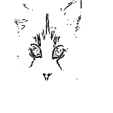
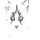
Fig. 2 shows the thresholded edge images of Fig. 1. We can see both binary images are almost the same, which indicates binary features can be taken as shape-like features to enhance the robustness of DCNN models. In this paper, a shallow binary feature module (SBFM for short) is proposed to extract the binary features of the input images, which stacks two types of layers–Sobel layer and threshold layer. In Sobel layer, there are four parallel feature maps which represent horizontal, vertical, and diagonal edge features respectively [9, 10]. And in threshold layer, it turns the learnt edge features from Sobel layers to the binary features, which then are feeded into the fully connected layers for classification with the features learnt by the backbones. SBFM is lightweight and can be integrated into any popular backbone, e.g., VGG [11] and ResNet [12]. We integrate SBFM into VGG16 and ResNet34, respectively. The experimental results on CIFAR-10, TinyImageNet, and Cats-and-dogs datasets show the training accuracy, test accuracy, and training time of the SBFM integrated models are on a par with those of original ones, and when attacked by FGSM [1] with $\epsilon=8/255$, the SBFM integrated models can achieve averagely 35% higher classification accuracy than the original ones, and 75% classification accuracy in CIFAR-10 and TinyImageNet datasets. The results demonstrate the binary features learnt by SBFM can enhance the robustness of DCNN models notably.

(a) Thresholded edge image for clean cat

(b) Thresholded edge image for adversarial cat

Figure 2: Thresholded edge images of Fig. 1.

The contributions of this paper can be summarized as follows:

1. We first raise the question ”can a DCNN model learn certain features which are insensitive to small perturbations, and further defend itself no matter what attack methods are presented”, and make a beginning effort on this.

2. SBFM is proposed to learn binary features through Sobel layer and threshold layer, which is lightweight and can be integrated into any popular backbone.

3. Experimental results on multiple datasets show, when attacked by FGSM with $\epsilon=8/255$, the SBFM integrated models can achieve averagely 35% higher accuracy compared to the original ones, and 75% classification accuracy n CIFAR-10 and TinyImageNet datasets.

II Related Work

Adversarial Training. AT is a widely used approach to enhance the robustness of DCNN models by generating AEs during each training step. Tsipras et al. [13] found there exists a tradeoff between robustness and standard accuracy of the models generated by AT, due to the robust classifiers learning a different feature representation compared to the clean classifiers. Madry et al. [14] proposed an approximated solution framework to the optimization problems of AT, and found PGD-based AT can produce models defending themselves against the first-order adversaries. Kannan et al. [15] investigated the effectiveness of AT at the scale of ImageNet [16], and proposed a logit pairing AT training method to tackle the tradeoff between robust accuracy and clean accuracy. Wong et al. [17] accelerated the training process using FGSM attack with random initialization instead of PGD attack [18], and reached significantly lower cost. Xu et al. [19] proposed a novel attack method which can make a stronger perturbation to the input images, resulting in the robustness of models by AT using this attack method is improved. Li et al. [20] revealed a link between fast growing gradient of examples and catastrophic overfitting during robust training, and proposed a subspace AT method to mitigate the overfitting and increase the robustness. Dabouei et al. [21] found the gradient norm in AT is higher than natural training, which hinders the training convergence of outer optimization of AT. And they proposed a gradient regularization method to improve the performance of AT. AT improves the robustness of the DCNN models by generating AEs using one specific attack method. However, in practice, the models trained by AT may be still vulnerable when facing the novel attack methods.

Part-based Model. Li eg al. [7] argued one reason that DCNN models are prone to be attacked is they are trained only on category labels, not on the part-based knowledge as humans do. They proposed a object recognition model, which first segments the parts of objects, scores the segmentations based on human knowledge, and final outputs the classification results based on the scores. This part-based model shows better robustness than classic recognition models across various attack settings. Sitawarin et al. [8] also thought richer annotation information can help learn more robust features. They proposed a part segmentation model with a head classifier trained end-to-end. The model first segments objects into parts, and then makes predictions based on the parts.

In both works, the shape-like features are leant to enhance the robustness of DCNN models remarkably. However, the proposed part-based models require the detailed segmentation annotation of objects and prior knowledge, and are hard to be combined with the existing recognition or detection architectures. In this paper, we propose a binary feature learning module which can be integrated into any popular backbone and enhance the robustness of DCNN models notably.

III Shallow Binary Feature Module

In this section, we give a detailed description of SBFM, which is lightweight and can be integrated into any popular backbone. SBFM stacks two types of layers–Sobel layer and threshold layer. In Sobel layer, four parallel feature maps are learnt to represent horizontal, vertical, and diagonal features respectively. In threshold layer, it sets a threshold to turn the features from Sobel layers into binary features. The architecture of a SBFM integrated classification model is shown in Fig. 3.

Figure 3: The architecture of a SBFM integrated classification model.

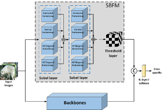
Sobel Layer. A Sobel layer consists of four parallel feature maps, i.e., horizontal feature maps, vertical feature maps, positive diagonal feature maps, and negative diagonal feature maps. For each feature map, a constrained kernel is designed to ensure the corresponding features can be learnt. Taking kernel size of 3 by 3 for example, the four types of kernel are shown in Fig. 4.

(a) Horizontal kernel

(b) Vertical kernel

(c) Positive diagonal kernel

(d) Negative diagonal kernel

Figure 4: Four types of kernels of Sobel layer.

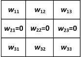
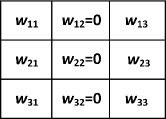
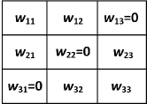
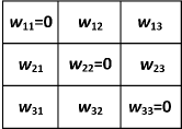
For horizontal kernel in Fig. 4(a),

$$w_{ij}\left\{\begin{array}[]{ll}\in\textrm{[0, 1]}&\mbox{if \emph{i} = 1, \emph{j} = 1, 2, 3},\\ =\textrm{0}&\mbox{if \emph{i} = 2, \emph{j} = 1, 2, 3},\\ \in\textrm{[-1, 0]}&\mbox{if \emph{i} = 3, \emph{j} = 1, 2, 3},\\ \end{array}\right.$$ (1)

For vertical kernel in Fig. 4(b),

$$w_{ij}\left\{\begin{array}[]{ll}\in\textrm{[0, 1]}&\mbox{if \emph{j} = 1, \emph{i} = 1, 2, 3},\\ =\textrm{0}&\mbox{if \emph{j} = 2, \emph{i} = 1, 2, 3},\\ \in\textrm{[-1, 0]}&\mbox{if \emph{j} = 3, \emph{i} = 1, 2, 3},\\ \end{array}\right.$$ (2)

For positive diagonal kernel in Fig. 4(c),

$$w_{ij}\left\{\begin{array}[]{ll}\in\textrm{[0, 1]}&\mbox{if (\emph{i}, \emph{j}) $\in$ \{(1, 1), (1, 2), (2, 1) \}},\\ =\textrm{0}&\mbox{if (\emph{i}, \emph{j}) $\in$ \{(1, 3), (2, 2), (3, 1) \}},\\ \in\textrm{[-1, 0]}&\mbox{if (\emph{i}, \emph{j}) $\in$ \{(2, 3), (3, 2), (3, 3) \}},\\ \end{array}\right.$$ (3)

For negative diagonal kernel in Fig. 4(d),

$$w_{ij}\left\{\begin{array}[]{ll}\in\textrm{[0, 1]}&\mbox{if (\emph{i}, \emph{j}) $\in$ \{(1, 2), (1, 3), (2, 3) \}},\\ =\textrm{0}&\mbox{if (\emph{i}, \emph{j}) $\in$ \{(1, 1), (2, 2), (3, 3) \}},\\ \in\textrm{[-1, 0]}&\mbox{if (\emph{i}, \emph{j}) $\in$ \{(2, 1), (3, 1), (3, 2) \}},\\ \end{array}\right.$$ (4)

The output of a Sobel layer is the addition of the four feature maps.

Threshold Layer. Features computed from the last Sobel layer are feeded into threshold layer, which can be denoted as $\textbf{x}^{in}$ $\in$ $R^{N\times P\times Q}$, where $N$ is the number of channels of the feature map, and $P$ and $Q$ are the width and height of each channel respectively. We set a threshold for each channel, and the features output from the threshold layer, $\textbf{x}^{out}$, can be computed using Eq. 5.

$$x_{ikj}^{out}=\left\{\begin{array}[]{ll}1&\mbox{if $x_{ikj}^{in}$ $\geq$ $t$ * $\max$($\textbf{x}_{i}^{in}$)},\\ 0&\mbox{if $x_{ikj}^{in}$ $<$ $t$ * $\max$($\textbf{x}_{i}^{in}$)},\\ \end{array}\\ \right.$$ (5)

where $i$ = 1,2,…,$N$, $k$ = 1,2,…,$P$, and $j$ = 1,2,…,$Q$. $t$ $\in$ [0, 1], and $\max$($\textbf{x}_{i}^{in}$) represents the maximum value of channel $i$.

It is obvious to see that, the higher $t$, the less binary features obtained; the smaller $t$, the more binary features obtained.

IV Experiments

In this section, we conduct experiments to examine whether the SBFM integrated VGG16 (VGG16-SBFM) and ResNet34 (ResNet34-SBFM) are more robust than the original ones on CIFAR-10 [22], TinyImageNet [23], and Cats-and-Dogs [24] datasets. Firstly, the effects of SBFM on model training are described. Secondly, the robustness of the SBFM integrated models and the original ones are compared under FGSM attack. And thirdly, the impacts of the number of Sobel layers and threshold on the robustness of the SBFM integrated models are analyzed. All experiments are coded using TensorFlow, and run on Intel i9 cpu of 3.6GHz with 64 GB RAM. One TITAN XP GPU is employed.

IV-A Datasets

CIFAR-10. CIFAR-10 dataset includes 10 classes, each of which has 6,000 training images, and 1,000 test images. In experiments, 10% training images in each class are taken as validation images. The resolution of images is 32$\times$ 32.

TinyImageNet. TinyImageNet dataset includes 200 classes, each of which has 500 training images, and 50 validation images. In experiments, validation images are taken as test images, and 10% training images in each class are taken as validation images. The resolution of images is 64$\times$ 64.

Cats-and-Dogs. Cats-and-Dogs dataset includes 2 classes, each of which has 12,500 images. In experiments, 9,000, 1,000, and 2,500 images in each class are taken as training, validation, and test images, respectively. The resolution of images is resized to 224$\times$ 224.

IV-B Effects of SBFM on model training

We examine the effects of SBFM on model training by comparing three metrics between the SBFM integrated models and the original ones, i.e., training accuracy, test accuracy, and training time per epoch. In SBFM, there are generally two parameters to be set–one is the number of Sobel layers, denoted as $l$, and the other is the proportion coefficient for threshold layer, denoted as $t$. On CIFAR-10 dataset, $l$ and $t$ are set to 3 and 0.8, respectively, for both VGG16-SBFM and ResNet34-SBFM. On TinyImageNet and Cats-and-Dogs dataset, $l$ and $t$ are set to 2 and 0.8 for VGG16-SBFM, and 3 and 0.8 for ResNet34-SBFM, respectively. The loss function, optimizer, the batch size, and the number of epochs are set to be the same. Each model is run for five times, and the average values are recorded. Table I shows the comparison of training performance between SBFM integrated models and the original ones. From the table, it is clear to see the SBFM integrated models are on a par with the original models on three metrics, which indicates SBFM has no side effect on model training and is lightweight.

	CIFAR-10			TinyImageNet			Cats-and-Dogs
	Tr.Acc.	Te.Acc.	TimePE	Tr.Acc.	Te.Acc.	TimePE	Tr.Acc.	Te.Acc.	TimePE
VGG16	99.17%	83.70%	18s	94.32%	33.84%	80s	97.64%	80.10%	14s
VGG16-SBFM	99.53%	82.95%	18s	92.03%	30.01%	95s	97.05%	83.17%	23s
ResNet34	99.32%	79.19%	48s	97.53%	30.80%	238s	96.32%	78.30%	85s
ResNet34-SBFM	99.48%	74.58%	48s	97.98%	26.31%	250s	95.64%	73.80%	92s

• Tr.Acc. stands for training accuracy. Te.Acc. stands for test accuracy. TimePE stands for training time per epoch.

TABLE I: Comparison of training performance between SBFM integrated models and the original ones.

IV-C Performance comparison between SBFM integrated models and original models under FGSM attack

We compare the classification accuracy between SBFM integrated models and original ones under FGSM attack, with $\epsilon$ set to 0.1/255, 0.5/255, 1/255, 2/255, 3/255, 5/255, and 8/255. $l$ and $t$ of the SBFM integrated models are set to the same values in Sec. IV-B. Each model is run for five times, and the average value is recorded.

Fig. 5-Fig. 7 show the changing curves of the classification accuracy for both SBFM integrated models and the original ones with the attack intensity $\epsilon$ increasing. From the figures, we can see that, in both CIFAR-10 and TinyImageNet datasets, the changing curves of SBFM integrated models are much more gentle compared to the original ones with the increase of $\epsilon$, showing the robustness is enhanced greatly after integrating SBFM. In Cats-and-Dogs dataset, the changing patterns of curves for both SBFM integrated models and the original ones are nearly the same, showing no notable advantage by SBFM for robustness enhancement. Here we make a note that, when training on Cats-and-Dogs dataset, the strides and pooling coefficients for SBFM are forced to set larger than those on CIFAR-10 and TinyImageNet datasets, due to the memory limitation. This may result in the poor performance of SBFM integrated models on Cats-and-Dogs dataset.

Figure 5: Changing curve of classification accuracy with the strengthening of the attack intensity $\epsilon$ on CIFAR-10.

Figure 6: Changing curve of classification accuracy with the strengthening of the attack intensity $\epsilon$ on TinyImageNet.

Figure 7: Changing curve of classification accuracy with the strengthening of the attack intensity $\epsilon$ on Cats-and-Dogs.

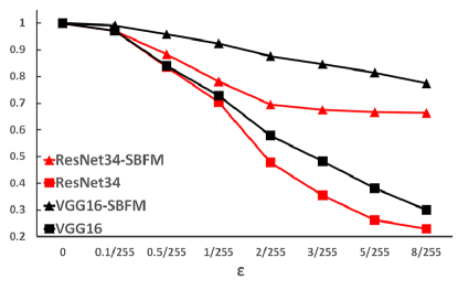
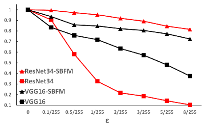
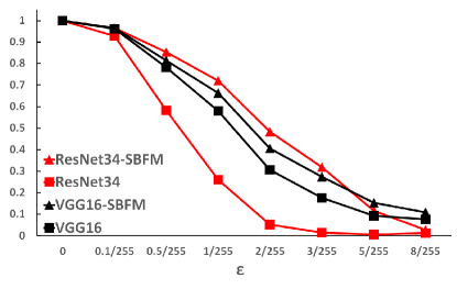
Table II shows the classification accuracy at $\epsilon$ = 8/255 for both SBFM integrated models and the original ones on three datasets. From the table, we can see that, on CIFAR-10, VGG16-SBFM is 47.43% higher accurate than VGG16, achieving 77.44% classification accuracy. ResNet34-SBFM is 43.46% higher accurate than ResNet34, achieving 66.41% classification accuracy. And on TinyImageNet dataset, VGG16-SBFM is 44.37% higher accurate than VGG16, achieving 72.38% classification accuracy. ResNet34-SBFM is 71.10% higher accurate than ResNet34, achieving 81.46% classification accuracy. The results demonstrate the binary features learnt by SBFM can enhance the robustness of DCNN models notably.

	CIFAR-10	TIN	CaD
VGG16	30.01%	37.65%	7.64%
VGG16-SBFM	77.44%	72.38%	10.95%
ResNet34	22.95%	10.36%	1.35%
ResNet34-SBFM	66.41%	81.46%	2.69%

• TIN stands for TinyImageNet. CaD stands for Cats-and-Dogs.

TABLE II: Comparison of classification accuracy between SBFM integrated models and original ones under FGSM attack with $\epsilon$ = 8/255.

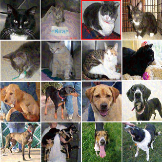
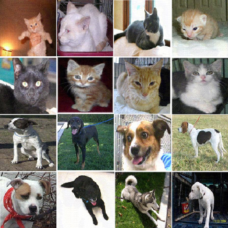
Fig. 8-Fig. 11 show the AEs of $\epsilon$ = 8/255 which can be classified correctly by the SBFM integrated models.

Figure 8: Correctly classified adversarial examples of TinyImageNet by VGG16-SBFM.

Figure 9: Correctly classified adversarial examples of TinyImageNet by ResNet34-SBFM.

Figure 10: Correctly classified adversarial examples of Cats-and-Dogs by VGG16-SBFM.

Figure 11: Correctly classified adversarial examples of Cats-and-Dogs by ResNet34-SBFM.

IV-D Impacts of the number of Sobel layers and threshold

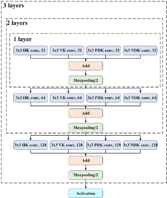
We examine the impacts of $l$ and $t$ settings on classification accuracy under $\epsilon$=8/255 attack. The values of $l$ and $t$ are set to 1, 2, 3, and 0.4, 0.6, 0.8 respectively. The loss function, optimizer, the batch size, and the number of epochs are set to be the same. Each model is run for five times, and the average value is recorded. Fig. 12 illustrates the architecture of SBFM with 1 Sobel layer, 2 Sobel layers, and 3 Sobel layers. Table III-Table VI describe the classification accuracy and training performance of SBFM integrated models under different settings of $l$ and $t$ on CIFAR-10, TinyImageNet, and Cats-and-Dogs datasets. From the tables, we can see that, the classification accuracy of the SBFM integrated models under attack varies distinctly with different $l$ and $t$ settings, e.g., on CIFAR-10 dataset, ResNet34-SBFM reaches 64.19% classification accuracy at $l$=2 and $t$=0.8, while achieving 17.19% classification accuracy at $l$=2 and $t$=0.4. And in addition, the test accuracy of the SBFM integrated models is not satisfying at certain settings of $l$ and $t$, e.g., in CIFAR-10 dataset, test accuracy of ResNet34-SBFM is 64.53% at $l$=2 and $t$=0.4, compared to 78.73% at $l$=2 and $t$=0.8.

Figure 12: SBFM with 1 Sobel layer, 2 Sobel layers, and 3 Sobel layers. HK stands for horizontal kernel. VK stands for vertical kernel. PDK stands for positive diagonal kernel. NDK stands for negative diagonal kernel.

	l = 1			l = 2			l = 3
	t = 0.4	t = 0.6	t = 0.8	t = 0.4	t = 0.6	t = 0.8	t = 0.4	t = 0.6	t = 0.8
VGG16-SBFM	40.43%	47.81%	47.22%	49.07%	57.36%	52.21%	79.96%	75.08%	77.44%
ResNet34-SBFM	62.79%	60.75%	58.71%	17.19%	29.74	64.19%	68.67%	67.65%	66.41%

TABLE III: Comparison of classification accuracy of the SBFM integrated models for different $l$ and $t$ settings on CIFAR-10 dataset. $\epsilon$=8/255.

	l = 1			l = 2			l = 3
	t = 0.4	t = 0.6	t = 0.8	t = 0.4	t = 0.6	t = 0.8	t = 0.4	t = 0.6	t = 0.8
VGG16-SBFM	27.62%	31.50%	31.69%	47.28%	63.86%	72.38%	35.53%	44.68%	50.97%
ResNet34-SBFM	5.21%	25.35%	20.81%	40.23%	56.68%	65.54%	84.56%	86.86%	81.46%

TABLE IV: Comparison of classification accuracy of the SBFM integrated models for different $l$ and $t$ settings on TinyImageNet dataset. $\epsilon$=8/255.

	l = 1			l = 2			l = 3
	t = 0.4	t = 0.6	t = 0.8	t = 0.4	t = 0.6	t = 0.8	t = 0.4	t = 0.6	t = 0.8
VGG16-SBFM	4.83%	18.05%	11.66%	26.31%	24.68%	10.95%	45.28%	10.59%	7.69%
ResNet34-SBFM	1.25%	1.28%	1.82%	0.34%	1.00%	5.73%	0.05%	0.65%	2.69%

TABLE V: Comparison of classification accuracy of the SBFM integrated models for different $l$ and $t$ settings on Cats-and-Dogs dataset. $\epsilon$=8/255.

	CIFAR-10			TinyImageNet			Cats-and-Dogs
	Tr.Acc.	Te.Acc.	TimePE	Tr.Acc.	Te.Acc.	TimePE	Tr.Acc.	Te.Acc.	TimePE
VGG16-SBFM, $l$=1, $t$=0.4	99.17%	82.50%	23s	95.96%	32.89%	81s	99.58%	74.77%	22s
VGG16-SBFM, $l$=1, $t$=0.6	99.32%	83.07%	23s	95.56%	30.63%	80s	96.59%	66.80%	22s
VGG16-SBFM, $l$=1, $t$=0.8	99.50%	83.99%	23s	96.44%	30.47%	80s	98.48%	75.90%	22s
VGG16-SBFM, $l$=2, $t$=0.4	99.21%	83.43%	22s	90.80%	31.14%	92s	98.88%	71.07%	20s
VGG16-SBFM, $l$=2, $t$=0.6	98.87%	83.12%	22s	95.42%	27.35%	93s	98.90%	67.23%	20s
VGG16-SBFM, $l$=2, $t$=0.8	99.00%	83.24%	22s	92.28%	30.01%	92s	99.34%	83.17%	20s
VGG16-SBFM, $l$=3, $t$=0.4	99.17%	83.48%	18s	56.32%	33.00%	92s	99.04%	64.27%	23s
VGG16-SBFM, $l$=3, $t$=0.6	99.32%	83.58%	18s	91.15%	30.77%	92s	99.17%	82.47%	23s
VGG16-SBFM, $l$=3, $t$=0.8	99.19%	82.59%	18s	92.03%	30.20%	92s	99.64%	82.80%	23s
ResNet34-SBFM, $l$=1, $t$=0.4	99.59%	72.80%	48s	98.54%	15.77%	247s	97.89%	62.07%	86s
ResNet34-SBFM, $l$=1, $t$=0.6	99.43%	77.92%	48s	98.33%	27.81%	246s	98.12%	60.77%	87s
ResNet34-SBFM, $l$=1, $t$=0.8	99.32%	78.96%	48s	98.31%	24.93%	246s	98.04%	56.43%	87s
ResNet34-SBFM, $l$=2, $t$=0.4	99.50%	64.53%	50s	98.22%	22.36%	250s	98.69%	71.07%	89s
ResNet34-SBFM, $l$=2, $t$=0.6	99.34%	65.87%	50s	97.98%	24.20%	250s	98.12%	68.17%	89s
ResNet34-SBFM, $l$=2, $t$=0.8	99.67%	78.73%	50s	97.87%	21.73%	249s	97.99%	65.87%	89s
ResNet34-SBFM, $l$=3, $t$=0.4	99.43%	69.49%	51s	97.65%	21.78%	254s	96.03%	75.10%	91s
ResNet34-SBFM, $l$=3, $t$=0.6	99.17%	73.40%	51s	96.92%	23.68%	254s	96.64%	71.33%	90s
ResNet34-SBFM, $l$=3, $t$=0.8	99.27%	74.58%	51s	97.92%	26.31%	256s	97.13%	73.80%	91s

• Tr.Acc. stands for training accuracy. Te.Acc. stands for test accuracy. TimePE stands for training time per epoch.

TABLE VI: Comparison of training performance between SBFM integrated models with different $l$ and $t$ settings.

V Discussions

The experimental results from Section IV shows SBFM has no side effect on model training, and it is lightweight and can be integrated into any backbone. Furthermore, the binary features learnt by the SBFM can enhance the robustness of DCNN models notably.

Here, we want to emphasize that, in this paper, a heuristic combination form of texture features and binary features (shown in Fig. 3) is introduced. We believe it is worthwhile to explore other effective and efficient combination forms of both features to enhance the robustness of DCNN models. Also, from the experimental results, it can be seen that, the performance of SBFM integrated models under attack changes distinctly for different parameter settings, and the generalization ability of the trained SBFM integrated models is relatively weak at certain parameter settings. It hints us that it is of great importance to design an optimization framework for parameter searching to yield the SBFM integrated models with exceptional classification accuracy under attack and satisfying generalization ability.

VI Conclusions

Enhancing the robustness of DCNN models is of great significance for the safety-critical applications in the real world. In this paper, we first raise the question ”can a DCNN model learn certain features which are insensitive to small perturbations, and further defend itself no matter what attack methods are presented”, and make a beginning effort to answer it. A shallow binary feature module is proposed, which is lightweight and can be integrated into any popular backbone. The experimental results on multiple datasets show the binary features learnt by the shallow binary feature module can enhance the robustness of DCNN models notably. In future’s work, we endeavor to explore other effective and efficient combination forms of binary features and texture features, and design an optimization framework for the parameter searching to yield models with good performance under attack and generalization ability. The work in this paper shows it is promising to enhance the robustness of DCNN models through feature learning.

References

- [1] I. J. Goodfellow, J. Shlens, and C. Szegedy, “Explaining and harnessing adversarial examples,” in International Conference on Learning Representations (ICLR), 2015.
- [2] C. Szegedy, W. Zaremba, I. Sutskever, J. Bruna, D. Erhan, I. Goodfellow, and R. Fergus, “Intriguing properties of neural networks,” in International Conference on Learning Representations (ICLR), 2014.
- [3] M. Andriushchenko and N. Flammarion, “Understanding and improving fast adversarial training,” in Proceedings of the 34th International Conference on Neural Information Processing Systems, 2020.
- [4] T. Bai, J. Luo, J. Zhao, B. Wen, and Q. Wang, “Recent advances in adversarial training for adversarial robustness,” in Proceedings of the Thirtieth International Joint Conference on Artificial Intelligence, IJCAI-21, 2021, pp. 4312–4321. [Online]. Available: https://doi.org/10.24963/ijcai.2021/591
- [5] N. Carlini and D. Wagner, “Towards evaluating the robustness of neural networks,” in 2017 IEEE Symposium on Security and Privacy (SP), 2017, pp. 39–57.
- [6] H. Wang, A. Zhang, S. Zheng, X. Shi, M. Li, and Z. Wang, “Removing batch normalization boosts adversarial training,” in Proceedings of the 39th International Conference on Machine Learning, 2022, pp. 23 433–23 445.
- [7] X. Li, Z. Wang, B. Zhang, F. Sun, and X. Hu, “Recognizing object by components with human prior knowledge enhances adversarial robustness of deep neural networks,” IEEE Transactions on Pattern Analysis and Machine Intelligence, 2023.
- [8] C. Sitawarin, K. Pongmala, Y. Chen, N. Carlini, and D. Wagner, “Part-based models improve adversarial robustness,” arXiv preprint arXiv:2209.09117, 2022.
- [9] J. Kittler, “On the accuracy of the sobel edge detector,” Image and Vision Computing, vol. 1, no. 1, pp. 37–42, 1983.
- [10] H. Xiao, S. Xiao, G. Ma, and C. Li, “Image sobel edge extraction algorithm accelerated by opencl,” JOURNAL OF SUPERCOMPUTING, vol. 78, no. 14, pp. 16 236–16 265, SEP 2022.
- [11] K. Simonyan and A. Zisserman, “Very deep convolutional networks for large-scale image recognition,” in International Conference on Learning Representations (ICLR), 2015.
- [12] K. He, X. Zhang, S. Ren, and J. Sun, “Deep residual learning for image recognition,” in Proceedings of the IEEE conference on computer vision and pattern recognition, 2016, pp. 770–778.
- [13] D. Tsipras, S. Santurkar, L. Engstrom, A. Turner, and A. Madry, “Robustness may be at odds with accuracy,” in International Conference on Learning Representations (ICLR), 2019.
- [14] A. Madry, A. Makelov, L. Schmidt, D. Tsipras, and A. Vladu, “Towards deep learning models resistant to adversarial attacks,” in International Conference on Learning Representations (ICLR), 2018.
- [15] H. Kannan, A. Kurakin, and I. Goodfellow, “Adversarial logit pairing,” in Proceedings of the 32th International Conference on Neural Information Processing Systems, 2018.
- [16] J. Deng, W. Dong, R. Socher, L.-J. Li, K. Li, and L. Fei-Fei, “Imagenet: A large-scale hierarchical image database,” in IEEE conference on computer vision and pattern recognition. Ieee, 2009, pp. 248–255.
- [17] E. Wong, L. Rice, and J. Z. Kolter, “Fast is better than free: Revisiting adversarial training,” in International Conference on Learning Representations (ICLR), 2020.
- [18] A. Kurakin, I. Goodfellow, and S. Bengio, “Adversarial machine learning at scale,” in International Conference on Learning Representations (ICLR), 2017.
- [19] Z. Xu, G. Zhu, C. Meng, S. Cui, Z. Ying, W. Wang, M. Gu, and Y. Huang, “A2: Efficient automated attacker for boosting adversarial training,” in Proceedings of the 36th International Conference on Neural Information Processing Systems, 2022.
- [20] T. Li, Y. Wu, S. Chen, K. Fang, and X. Huang, “Subspace adversarial training,” in Proceedings of the IEEE/CVF Conference on Computer Vision and Pattern Recognition, 2022, pp. 13 409–13 418.
- [21] A. Dabouei, F. Taherkhani, S. Soleymani, and N. M. Nasrabadi, “Revisiting outer optimization in adversarial training,” in Computer Vision–ECCV 2022: 17th European Conference, Tel Aviv, Israel, October 23–27, 2022, Proceedings, Part V. Springer, 2022, pp. 244–261.
- [22] A. Krizhevsky, G. Hinton et al., “Learning multiple layers of features from tiny images,” 2009.
- [23] Y. Le and X. Yang, “Tiny imagenet visual recognition challenge,” CS 231N, vol. 7, no. 7, p. 3, 2015.
- [24] J. Elson, J. J. Douceur, J. Howell, and J. Saul, “Asirra: A captcha that exploits interest-aligned manual image categorization,” in Proceedings of 14th ACM Conference on Computer and Communications Security (CCS), October 2007.