To the theory of phase transition of a binary solution into an inhomogeneous phase

Abstract

In the framework of the theoretical model of the phase transition of binary solutions into spatially inhomogeneous states proposed earlier by the authors [1], which takes into account nonlinear effects, the role of the cubic in concentration term in the expansion of free energy was studied. It is shown that taking into account the cubic term contributes to the stabilization of a homogeneous state. The existence of two inhomogeneous phases in an isotropic medium, considered in [1], proves to be possible only at half the concentration of the solution. The contribution of inhomogeneity effects to thermodynamic quantities is calculated. Phase transitions from a homogeneous state and between inhomogeneous phases are second-order phase transitions.
Key words: binary solution, concentration, phase transition, stratification, concentration waves, phase diagram, free energy, entropy, heat capacity

I Introduction

In [1], the authors proposed a model for the phase transition of a binary solution into an inhomogeneous state and studied the thermodynamics of this process. This work was a development of the approach proposed earlier in articles [2–5]. A feature of the model considered in [1] is that it assumes, as is the case in real conditions, a fixed average concentration. The free energy of the solution is chosen as a polynomial of the fourth degree in the concentration fluctuations. In [1] the authors analyzed in detail the particular case when there is absent a cubic term in the expansion of free energy, which can be realized in crystals of a certain crystal symmetry [6]. It was shown that in this case the solution, as a result of the loss of stability of a spatially homogeneous state, can at an arbitrary concentration go either into a state with a concentration wave (W -phase), or into a state with stratification which is described by a solution in the form of a ”kink” (K -phase).

The purpose of this work is to study the influence of the term in the free energy, which is cubic with respect to concentration fluctuations, on the character of transition to an inhomogeneous state. Within the framework of the model of an isotropic medium, it is shown that taking into account the cubic contribution leads to the stabilization of a homogeneous state. The transition to an inhomogeneous state proves to be possible only at the half concentration, when the cubic in concentration term vanishes. At other concentrations there also exist coordinate-dependent solutions in theory, but they do not satisfy the requirement of conservation of the number of particles, and therefore are not realized physically. The contribution of inhomogeneity to thermodynamic characteristics of a binary solution is studied and it is shown that transitions between phases are second-order transitions with a jump in the heat capacity.

II Formulation of the task

We consider a solution of particles of two types, the number of which is $N_{1}$ and $N_{2}$, occupying a constant volume $V$. In the isotropic approximation and for a spatially homogeneous state, the thermodynamic properties of such a solution can be described using a free energy, which is a function of temperature $T$, volume $V$, and depends on the number of particles of each component: $F=F(T,V,N_{1},N_{2})$. Sometimes it is more convenient to proceed to the description using the total number of particles $N=N_{1}+N_{2}$ and the concentration $c_{1}\equiv\overline{c}=N_{1}/N$ of one of the components. As is known [7], in a spatially homogeneous state the free energy for the one-component case can be represented as $F=N\varphi(n,T)$. In the case of two components, a similar relationship will take the form $F=N\varphi(n,T,c)$, where $n=N/V$ is the total density of the number of particles, which will be assumed to be constant. In a spatially inhomogeneous state, the concentration $c=c({\bf r})$ will be considered as a continuous function of spatial coordinates. In this case, the total free energy will be written in the form

$$\begin{array}[]{l}\displaystyle{\overline{F}=n\!\int\!\varphi\big{(}T,n,\overline{c}\,;\delta c({\bf r}),\nabla\delta c({\bf r})\big{)}\,d{\bf r}.}\end{array}$$ (1)

Thermodynamic potential (1) is a potential with incomplete thermodynamic equilibrium. The temperature and density in it are assumed to be equilibrium and independent of the coordinates, and the order parameter, in our case it is the deviation of the concentration from its equilibrium average value $\delta c({\bf r})=c({\bf r})-\overline{c}$, should be found as a result of varying the free energy (1) with respect to the concentration from the condition $\delta\overline{F}=0$. This leads to the equation

$$\begin{array}[]{l}\displaystyle{\frac{\partial\varphi}{\partial\delta c}-\nabla\frac{\partial\varphi}{\partial\nabla\delta c}=0.}\end{array}$$ (2)

Usually, the number of particles in a system is assumed to be fixed, since it is determined by the composition of a sample; therefore, we will consider the average concentration $\overline{c}=N_{1}/N$ as a fixed parameter. By virtue of the requirement of conservation of the total number of particles, the following conditions must be satisfied

$$\begin{array}[]{l}\displaystyle{\frac{1}{V}\!\int\!\delta c({\bf r};T,n,\overline{c})\,d{\bf r}=0,\qquad\overline{c}=\frac{1}{V}\!\int\!c({\bf r};T,n,\overline{c})\,d{\bf r}.}\end{array}$$ (3)

Solutions of equation (2), which depend on temperature, density and the average concentration $\delta c=\delta c({\bf r};T,n,\overline{c})$, should be substituted into the expression for the free energy (1). As a result, we obtain the formula for the equilibrium free energy

$$\begin{array}[]{l}\displaystyle{F=n\!\int\!\varphi\big{(}T,n,\overline{c}\,;\delta c({\bf r};T,n,\overline{c}),\nabla\delta c({\bf r};T,n,\overline{c})\big{)}\,d{\bf r}.}\end{array}$$ (4)

The total entropy of the solution is determined through the derivative of the equilibrium free energy (4) with respect to temperature at constant parameters $n$ and $\overline{c}$:

$$\begin{array}[]{l}\displaystyle{S=-\frac{\partial F}{\partial T}=-n\int\frac{\partial^{\prime}\varphi}{\partial T}\,d{\bf r}.}\end{array}$$ (5)

In this case, due to condition (2), only the explicit dependence of $\varphi$ on temperature should be differentiated, which is marked in (5) with a prime. The equilibrium total energy of the solution is determined by the usual formula:

$$\begin{array}[]{l}\displaystyle{E=F+TS=n\int\!\left(\varphi-T\frac{\partial^{\prime}\varphi}{\partial T}\right)\!d{\bf r}.}\end{array}$$ (6)

In the proposed model, we choose the free energy density as an expansion in powers of the concentration fluctuation up to the fourth power inclusively:

$$\begin{array}[]{l}\displaystyle{\varphi=\varphi_{0}(T,n,\overline{c})+\frac{K}{2}\big{(}\nabla\delta c\big{)}^{2}+a_{2}\frac{(\delta c)^{2}}{2}+a_{3}\frac{(\delta c)^{3}}{3}+a_{4}\frac{(\delta c)^{4}}{4}.}\end{array}$$ (7)

The first term $\varphi_{0}(T,n,\overline{c})$ in (7) describes the contribution of the homogeneous state to the total free energy. In what follows, we will be interested in the effects associated with the inhomogeneity of a state. The linear term in (7) drops out due to the conservation condition (3). The coefficients in the expansion (7) depend, generally speaking, on the temperature, density, and also the average concentration $a_{i}=a_{i}(T,n,\overline{c})$, $K=K(T,n,\overline{c})$. To ensure the stability of the homogeneous state at high temperatures, the coefficients $K$ and $a_{4}$ should be considered positive, and the coefficient $a_{3}$ can be either positive or negative. Suppose that the coefficient $a_{2}$ changes sign at a certain temperature $T_{p}$, becoming negative at $T<T_{p}$. This temperature is also a function of the average concentration and density $T_{p}=T_{p}(\overline{c},n)$. As will be seen later, one can use the linear approximation $a_{2}=a_{0}\tau,\,\,\tau\equiv(T-T_{p})\big{/}T_{p}\,\,(a_{0}>0)$. For the free energy density of the form (7), formula (2) leads to the equation

$$\begin{array}[]{l}\displaystyle{K\Delta\delta c=a_{2}\delta c+a_{3}(\delta c)^{2}+a_{4}(\delta c)^{3}.}\end{array}$$ (8)

Among all possible solutions of this nonlinear equation, only those ones are physically realizable for which $0\leq c({\bf r})\leq 1$.

The explicit form of the phenomenological parameters entering into expansion (7) and their dependence on the average concentration, temperature, and density can be found using the well-known representation of the free energy [6, 8], which in the considered case of an isotropic medium can be represented as

$$\begin{array}[]{l}\displaystyle{\overline{F}=\frac{n^{2}}{2}\!\int\!d{\bf r}d{\bf r}^{\prime}V\big{(}|{\bf r}-{\bf r}^{\prime}|\big{)}c({\bf r})c({\bf r}^{\prime})+nT\!\int\!d{\bf r}\Big{[}c({\bf r})\ln c({\bf r})+\big{(}1-c({\bf r})\big{)}\ln\big{(}1-c({\bf r})\big{)}\Big{]},}\end{array}$$ (9)

where $V\big{(}|{\bf r}-{\bf r}^{\prime}|\big{)}$ is the interaction potential between particles. Expanding (9) in terms of small fluctuations $\delta c({\bf r})=c({\bf r})-\overline{c}$  and comparing with (4), (7), we obtain the following expressions for the expansion coefficients:

$$\begin{array}[]{ccc}\displaystyle{a_{2}=nV_{0}+\frac{T}{\overline{c}\,(1-\overline{c})},\qquad a_{3}=-\frac{(1-2\overline{c})}{2\,\overline{c}^{\,2}(1-\overline{c})^{2}}\,T,\qquad a_{4}=\frac{(1-3\overline{c}+3\overline{c}^{\,2})}{3\,\overline{c}^{\,3}(1-\overline{c})^{3}}\,T,\vspace{2mm}}\\ \displaystyle{K=-\frac{2\pi}{3}\,n\!\int\!dr\,r^{4}V(r),\qquad\varphi_{0}(T,\overline{c})=\frac{\overline{c}^{\,2}n}{2}\,V_{0}+T\big{[}\,\overline{c}\ln\overline{c}+(1-\overline{c})\ln(1-\overline{c})\big{]},}\end{array}$$ (10)

where $V_{0}=\!\int d{\bf r}V(r)$. The coefficient $a_{2}$ can change sign at some temperature becoming negative, if only $V_{0}<0$, so that the possibility of a loss of stability is determined by the nature of the interaction between atoms [1]. The temperature, at which the coefficient $a_{2}$ changes sign, is given by formula

$$\begin{array}[]{l}\displaystyle{T_{p}=n|V_{0}|\,\overline{c}\,(1-\overline{c}).}\end{array}$$ (11)

The coefficient $a_{2}=a_{0}\tau$ includes the parameter

$$\begin{array}[]{l}\displaystyle{a_{0}\equiv n|V_{0}|,}\end{array}$$ (12)

and the other two expansion coefficients have the form

$$\begin{array}[]{ccc}\displaystyle{a_{3}=-\frac{(1-2\overline{c})}{2\,\overline{c}^{\,2}(1-\overline{c})^{2}}\,T,\qquad a_{4}=\frac{(1-3\overline{c}+3\overline{c}^{\,2})}{3\,\overline{c}^{\,3}(1-\overline{c})^{3}}\,T.}\end{array}$$ (13)

The coefficient $K$ in this model does not depend on temperature. We represent the coefficients (13) as $a_{3}\equiv-Tq_{3}(\overline{c})$, $a_{4}\equiv Tq_{4}(\overline{c})$,where functions are introduced which depend only on the average concentration:

$$\begin{array}[]{ccc}\displaystyle{q_{3}(\overline{c})\equiv\frac{(1-2\overline{c})}{2\,\overline{c}^{\,2}(1-\overline{c})^{2}},\qquad q_{4}(\overline{c})\equiv\frac{(1-3\overline{c}+3\overline{c}^{\,2})}{3\,\overline{c}^{\,3}(1-\overline{c})^{3}}.}\end{array}$$ (14)

In paper [1] the authors considered in detail the case when the coefficient $a_{3}=0$. As we can see, in the considered approximation of a homogeneous medium the coefficient at the cubic term in expansion (7) vanishes only at the average concentration $\overline{c}=1/2$.

III Transition to spatially inhomogeneous states

Let us consider the transitions of a binary solution to spatially inhomogeneous states, assuming that the concentration can depend only on one spatial coordinate $x$, which varies within the limits $-L/2\leq x\leq L/2$. In this one-dimensional case, the total free energy (1) can be written as

$$\begin{array}[]{l}\displaystyle{\overline{F}=nA\!\int\!dx\left[\frac{K}{2}\left(\frac{d\,\delta c}{dx}\right)^{2}+a_{2}\frac{(\delta c)^{2}}{2}+a_{3}\frac{(\delta c)^{3}}{3}+a_{4}\frac{(\delta c)^{4}}{4}\right],}\end{array}$$ (15)

where $A$ is the area of a sample, the normal to which is parallel to the $x$ axis. Equation (8) in this case takes the form

$$\begin{array}[]{l}\displaystyle{K\frac{d^{2}\delta c}{dx^{2}}=a_{2}\delta c+a_{3}(\delta c)^{2}+a_{4}(\delta c)^{3}.}\end{array}$$ (16)

The first integral of this equation is

$$\begin{array}[]{l}\displaystyle{\frac{K}{2}\!\left(\frac{d\,\delta c}{dx}\right)^{2}=C-U(\delta c),}\end{array}$$ (17)

where $C$ is the constant of integration, and

$$\begin{array}[]{l}\displaystyle{U(\delta c)=-a_{4}\frac{(\delta c)^{4}}{4}-a_{3}\frac{(\delta c)^{3}}{3}-a_{2}\frac{(\delta c)^{2}}{2}.}\end{array}$$ (18)

Equation (17) is similar to the equation of motion of a material point in an external field $U(\delta c)$ (18) with energy $C$. Taking into account formulas (12) – (14), the field (18) can be represented as $U(\delta c)\equiv Tq_{4}\bar{U}(c)\big{/}4$:

$$\begin{array}[]{ccc}\displaystyle{\bar{U}(c)=-\Big{[}(\delta c)^{2}-2q(\overline{c})(\delta c)+p(\overline{c})\frac{\tau}{1+\tau}\Big{]}(\delta c)^{2}=-(c-c_{01})(c-c_{02})(c-\overline{c})^{2},\vspace{2mm}}\\ \end{array}$$ (19)

where

$$\begin{array}[]{ccc}\displaystyle{q(\overline{c})\equiv\frac{2}{3}\frac{q_{3}}{q_{4}}\equiv\frac{(1-2\overline{c})\,\overline{c}\,(1-\overline{c})}{(1-3\overline{c}+3\overline{c}^{2})},\qquad p(\overline{c})=\frac{2a_{0}}{T_{p}q_{4}}\equiv\frac{6\overline{c}^{2}(1-\overline{c})^{2}}{(1-3\overline{c}+3\overline{c}^{2})}.}\end{array}$$ (20)

The concentrations at which the field vanishes are determined by the formulas

$$\begin{array}[]{ccc}\displaystyle{c_{0}=\overline{c},\qquad c_{01}=\overline{c}+q-D,\qquad c_{02}=\overline{c}+Q+D,}\end{array}$$ (21)

where

$$\begin{array}[]{ccc}\displaystyle{D\equiv D(\tau)\equiv\sqrt{\frac{p}{1+\tau_{C}}}\sqrt{\frac{\tau_{C}-\tau}{1+\tau}},}\end{array}$$ (22)

and temperature

$$\begin{array}[]{ccc}\displaystyle{\tau_{C}=\frac{6(1-3\overline{c}+3\overline{c}^{2})}{(5-14\overline{c}+14\overline{c}^{2})}-1}\end{array}$$ (23)

is found from the condition $\big{(}q^{2}\big{/}p\big{)}-\tau_{C}\big{/}(1+\tau_{C})=0$. Inhomogeneous phases can exist at temperatures $\tau<\tau_{C}$, when the radical expression in (22) is positive. As was noted, for $\overline{c}=1/2$ the cubic term in (18) vanishes, and the field $U(\delta c)$ becomes symmetric with respect to the axis $c=\overline{c}$. In this case $\tau_{C}=0$. This case was in detail considered by the authors earlier in [1]. At other concentrations $q\neq 0$, the field $U(\delta c)$ turns out to be asymmetric, and $\tau_{C}\neq 0$. The form of the function $\bar{U}(c)=-(c-c_{01})(c-c_{02})(c-\overline{c})^{2}$ (19) is shown in Fig. 1. Its maximums are located at the points

$$\begin{array}[]{ccc}\displaystyle{c_{m1}=\overline{c}+\frac{3}{4}\Big{(}q-\frac{1}{2}G\Big{)},\qquad c_{m2}=\overline{c}+\frac{3}{4}\Big{(}q+\frac{1}{2}G\Big{)},}\end{array}$$ (24)

where $G\equiv\frac{2}{3}\sqrt{q^{2}+8D^{2}}$. The field values in maximums:

$$\begin{array}[]{ccc}\displaystyle{\left.\begin{array}[]{l}\bar{U}(c_{m1})\\ \bar{U}(c_{m2})\end{array}\!\right\}=\frac{9}{16}\bigg{[}D^{2}-\frac{1}{16}\bigg{(}q\pm\frac{3}{2}G\bigg{)}^{\!2}\bigg{]}\!\bigg{(}q\mp\frac{1}{2}G\bigg{)}^{\!2}.}\end{array}$$ (25)

In the symmetric case (Fig. 1a) at $\overline{c}=1/2$, when $q=0$, we have $\bar{U}(c_{m1})=\bar{U}(c_{m2})=D^{2}\!\big{/}4$.

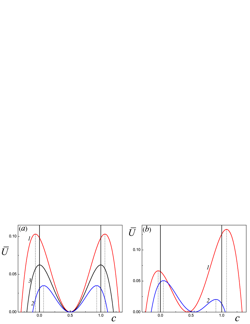
Figure 1: Form of the field $\bar{U}(c)$ (19): (​a) the symmetric case $\overline{c}=1/2$ at temperatures: (1) $\tau=-0.30$, (2) $\tau=-0.20$,
(3) $\tau=-0.25$; (​b) the asymmetric case: (1) $\overline{c}=0.45,\,\tau=-0.30$, (2) $\overline{c}=0.55,\,\tau=-0.20$.

There are two characteristic temperature regions, where the states are qualitatively different. In region I the values of concentration, at which the field (19) reaches its maximum, lie in the region of permissible values $0\leq c_{m1}<c_{m2}\leq 1$ (Fig. 1, curves 2). In region II the maximums lie outside the region of permissible values, so that the inequalities $c_{m1}<0$ and $c_{m2}>1$ are satisfied (Fig. 1, curves 1). The boundary temperature $T_{1}$ is determined by the conditions $c_{m1}=0,\,c_{m2}=1$ and $\overline{c}=1/2$, so that

$$\begin{array}[]{ccc}\displaystyle{\frac{T_{1}}{T_{p}}=\frac{3}{4}.}\end{array}$$ (26)

Thus, two temperature regions should be considered, where the states are qualitatively different: region I at $T_{1}<T<T_{p}$ , which was called the K -phase in [1], and region II at $0<T<T_{1}$ (the W -phase).

Equation (17) can be represented as

$$\begin{array}[]{l}\displaystyle{\xi^{2}\!\left(\frac{dz}{dx}\right)^{\!2}=(z-z_{1})(z-z_{2})(z-z_{3})(z-z_{4}).}\end{array}$$ (27)

Here and below we use the notation $z\equiv\delta c=c-\overline{c}$. In (27) $z_{1}\leq z_{2}\leq z_{3}\leq z_{4}$ are the real, arranged in ascending order roots of the algebraic equation

$$\begin{array}[]{l}\displaystyle{(z-q+D)(z-q-D)z^{2}+\varepsilon=0,}\end{array}$$ (28)

where $\varepsilon\equiv 4C\big{/}Tq_{4}$, and the correlation length $\xi$ in (27), which determines the size of the inhomogeneity region, is given by the relation

$$\begin{array}[]{l}\displaystyle{\xi^{2}\equiv\frac{2K}{Tq_{4}}.}\end{array}$$ (29)

If all real roots of equation (28) are different, then equation (27) has a periodic solution [9]

$$\begin{array}[]{l}\displaystyle{z(x)=z_{1}+\frac{r(z_{2}-z_{1})}{r-{\rm sn}^{2}\Big{(}\displaystyle{s\,\frac{x}{\xi}},m\Big{)}},}\end{array}$$ (30)

where ${\rm sn}\Big{(}\displaystyle{s\,\frac{x}{\xi}},m\Big{)}$ is the elliptic sine [10], and also

$$\begin{array}[]{l}\displaystyle{s\equiv\frac{1}{2}\sqrt{(z_{4}-z_{2})(z_{3}-z_{1})},\qquad r\equiv\frac{(z_{3}-z_{1})}{(z_{3}-z_{2})},\qquad m=\frac{(z_{3}-z_{2})(z_{4}-z_{1})}{(z_{4}-z_{2})(z_{3}-z_{1})}.}\end{array}$$ (31)

The period of the solution (30) is

$$\begin{array}[]{l}\displaystyle{L_{0}=\frac{2K(m)}{s}\,\xi,}\end{array}$$ (32)

where $K(m)$ the complete elliptic integral of the first kind [10].

IV The case of concentrations other than one-half. The matching condition

Let us first consider the case, when the average concentration is different from $\overline{c}=1/2$. In this case the cubic term in the free energy expansion (15) is nonzero. In this case, there exist periodic solutions in the form of concentration waves (30). In order for such solutions to describe real physical states, they must satisfy the matching condition (3), which follows from the requirement of conservation of the number of particles. In the one-dimensional case under consideration this condition has the form

$$\begin{array}[]{l}\displaystyle{\int_{0}^{L_{0}}\!z(x)dx=0,}\end{array}$$ (33)

where $L_{0}$ is the period (32). Using equation (27), the matching condition (33) can be represented as

$$\begin{array}[]{l}\displaystyle{J\big{(}\alpha,\beta\big{)}=J\big{(}\beta,\alpha\big{)},}\end{array}$$ (34)

where

$$\begin{array}[]{l}\displaystyle{J\big{(}\alpha,\beta\big{)}\equiv\int_{0}^{1}\!\frac{\lambda\,d\lambda}{\sqrt{\big{(}\cos^{-1}\!\alpha-\lambda\big{)}\big{(}1-\lambda\big{)}\big{(}\psi(\alpha,\beta)+\lambda\big{)}\big{(}\cos^{-1}\!\beta\,\cdot\psi(\alpha,\beta)+\lambda\big{)}}},}\end{array}$$ (35)

$\displaystyle{\psi(\alpha,\beta)=\frac{1+\cos\beta}{1+\cos\alpha}}$, and the angles $\alpha,\beta$ are defined through the ratios of the moduli of the roots of equation (28)

$$\begin{array}[]{l}\displaystyle{\frac{|z_{2}|}{|z_{1}|}=\cos\alpha,\qquad\frac{|z_{3}|}{|z_{4}|}=\cos\beta,}\end{array}$$ (36)

so that $0<\alpha,\,\beta<\pi/2$. An analysis shows that the condition (34) is satisfied in the single case $\alpha=\beta$, which corresponds to the symmetric case with concentration $\overline{c}=1/2$. For all other concentrations the condition (34) is not fulfilled and, consequently, such solutions are not realized.

In addition, aside from periodic solutions, when the condition $\varepsilon=\bar{U}(z_{m1})$ is fulfilled, where $z_{m1}=c_{m1}-\overline{c}$, Eq. (27) has a solution localized near an arbitrary point $x_{0}$, which can be represented as

$$\begin{array}[]{l}\displaystyle{\frac{1}{\sqrt{\big{(}a_{-}-a_{m}\big{)}\big{(}1-a_{m}\big{)}}}\,\ln\left[\frac{\left[\sqrt{\big{(}1-a_{m}\big{)}\big{(}a_{-}-\lambda\big{)}}-\sqrt{\big{(}a_{-}-a_{m}\big{)}\big{(}1-\lambda\big{)}}\,\right]^{\!2}}{|\lambda-a_{m}|}\right]=\pm z_{+}\frac{\big{(}x-x_{0}\big{)}}{\xi},}\end{array}$$ (37)

where $\lambda\equiv z\big{/}z_{+}$, $a_{m}\equiv z_{m1}\big{/}z_{+}$, $a_{-}\equiv z_{-}\big{/}z_{+}$, and here

$$\begin{array}[]{l}\displaystyle{z_{\pm}=\frac{1}{4}\left(q+\frac{3}{2}\,G\pm 2\sqrt{q^{2}+\frac{3}{2}\,qG}\right),\qquad z_{m1}=\frac{3}{8}\big{(}2q-G\big{)},}\end{array}$$ (38)

and as before $G\equiv\frac{2}{3}\sqrt{q^{2}+8D^{2}}$. This solution satisfies the matching condition (33) only in the limit of a sample of infinite length. Thus, at concentrations $\overline{c}\neq 1/2$, when the cubic term in the free energy is nonzero, the existing spatially inhomogeneous periodic and localized solutions do not satisfy the matching condition, and therefore cannot be physically realized.

V Thermodynamics of inhomogeneous states at $\overline{c}=1/2$

At the average concentration of $\overline{c}=1/2$ the cubic term in expansion (18) vanishes, since $q(1/2)=0$, and also in this case $q_{4}(1/2)=16/3$, $p(1/2)=3/2$. This case was considered in detail in the authors’ work [1]. Here, using a slightly different method, we present the main results and introduce some refinements into the method of describing the thermodynamics of inhomogeneous states.

In the temperature range $T_{1}<T<T_{p}$ (K -phase) at $\varepsilon=D^{4}\big{/}4$ there exist solutions in the form of a “kink”

$$\begin{array}[]{l}\displaystyle{z(x)=c(x)-\frac{1}{2}=\pm\frac{D}{\sqrt{2}}\,{\rm th}\bigg{(}\frac{D}{\sqrt{2}}\frac{x}{\xi}\bigg{)},}\end{array}$$ (39)

describing the stratification of the solution into regions with enriched and depleted concentrations, as well as, at $0<\varepsilon<D^{4}\big{/}4$, there exist solutions in the form of concentration waves

$$\begin{array}[]{l}\displaystyle{z(x)=c(x)-\frac{1}{2}=\pm\frac{D_{-}}{\sqrt{2}}\,{\rm sn}\bigg{(}\frac{D_{+}}{\sqrt{2}}\frac{x}{\xi};m\bigg{)},}\end{array}$$ (40)

where $m=D_{-}^{2}\big{/}D_{+}^{2}$, $D_{\pm}\equiv\sqrt{D^{2}\pm\sqrt{D^{4}-4\varepsilon}}$. In the temperature range $0<T<T_{1}$ (W -phase), there are physical solutions only in the form of concentration waves (40). Solutions (39), (40) satisfy the matching conditions (3), (33). Since $\varepsilon=D^{4}m\big{/}(1+m)^{2}$, $D_{+}^{2}=2D^{2}\big{/}(1+m)$, $D_{-}^{2}=2D^{2}m\big{/}(1+m)$, then each of the solutions is characterized by a parameter $m$ numerating all possible inhomogeneous states. For $m=1$, solution (40) transforms into the “kink” (39). The temperature dependence of quantities is mainly determined by the function (22), which in this case takes the form

$$\begin{array}[]{l}\displaystyle{D^{2}\equiv D^{2}(\tau)=-\frac{3}{2}\frac{\tau}{(1+\tau)}.}\end{array}$$ (41)

The width of the transition region in the “kink” $L_{K}(\tau)$ and the period of the concentration wave $L_{0}(m;\tau)$ are determined by the formulas

$$\begin{array}[]{l}\displaystyle{L_{K}\big{(}T\big{)}=\sqrt{2}\frac{\xi_{0}}{\sqrt{1-T/T_{p}}},\qquad L_{0}\big{(}m;T\big{)}=4K(m)\sqrt{1+m}\frac{\xi_{0}}{\sqrt{1-T/T_{p}}},}\end{array}$$ (42)

where $\xi_{0}^{2}=K/a_{0}$ is the temperature-independent correlation length, and $\xi^{2}=3\xi_{0}^{2}\big{/}2(1+\tau)$ (29). The temperature dependences of the lengths (42) are shown in Fig. 2. When approaching the homogeneous phase $T\rightarrow T_{p}$, they tend to infinity, and as $T\rightarrow 0$ they tend to a finite value $\sim\xi_{0}$.

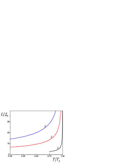
Figure 2: Temperature dependencies of the inhomogeneity dimensions: (1) “kink” width $L_{K}\big{(}T\big{)}$; wave period $L_{0}\big{(}m;T\big{)}$ for
(2) $m=0.1$ and (3) $m=0.9$.

Let us calculate the contribution of inhomogeneities to the thermodynamic quantities of the solution at the concentration $\overline{c}=1/2$. According to (5), (6), the entropy and energy can be represented in the form $S=-N\big{(}\partial\varphi_{0}/\partial T\big{)}+\delta S$, $E=N\big{(}\varphi_{0}-T\partial\varphi_{0}/\partial T\big{)}+\delta E$. We will be interested in the contributions of inhomogeneities to these quantities, defined by the formulas

$$\begin{array}[]{l}\displaystyle{\delta S=-\frac{4}{3}nA\Big{(}\frac{3}{2}J_{2}+J_{4}\Big{)},}\end{array}$$ (43)

$$\begin{array}[]{l}\displaystyle{\delta E=2nAT_{p}\big{(}\xi_{0}^{2}J-J_{2}\big{)}.}\end{array}$$ (44)

Here we introduce the notation of the following integrals:

$$\begin{array}[]{l}\displaystyle{J\equiv\int\!\bigg{(}\frac{dz}{dx}\bigg{)}^{\!2}dx,\qquad J_{2}\equiv\int\!z^{2}dx,\qquad J_{4}\equiv\int\!z^{4}dx.}\end{array}$$ (45)

For the “kink” (39) in a sample of length $L$, these integrals are as follows:

$$\begin{array}[]{l}\displaystyle{J=\frac{D^{3}}{\sqrt{2}\,\xi}\Big{(}{\rm th}y-\frac{1}{3}\,{\rm th}^{3}y\Big{)},\qquad J_{2}=\sqrt{2}D\xi\big{(}y-{\rm th}y\big{)},\qquad J_{4}=\frac{D^{3}}{\sqrt{2}}\,\xi\Big{(}y-{\rm th}y-\frac{1}{3}\,{\rm th}^{3}y\Big{)},}\end{array}$$ (46)

where $y\equiv\big{(}D\big{/}2\sqrt{2}\big{)}\big{(}L/\xi\big{)}$. For the concentration waves, integrals (45) are expressed by the formulas

$$\begin{array}[]{l}\displaystyle{J=\frac{L}{\xi^{2}}D^{4}\frac{m}{(1+m)^{2}}\frac{I_{0}(m)}{K(m)},\qquad J_{2}=LD^{2}\frac{m}{(1+m)}\frac{I_{2}(m)}{K(m)},\qquad J_{4}=LD^{4}\frac{m^{2}}{(1+m)^{2}}\frac{I_{4}(m)}{K(m)}.}\end{array}$$ (47)

Here

$$\begin{array}[]{ccc}\displaystyle{I_{0}(m)=\frac{1}{3m}\big{[}(m-1)K(m)+(m+1)E(m)\big{]},\vspace{2mm}}\\ \displaystyle{I_{2}(m)=\frac{1}{m}\big{[}K(m)+E(m)\big{]},\vspace{2mm}}\\ \displaystyle{I_{4}(m)=\frac{1}{3m^{2}}\big{[}(m+2)K(m)-2(m+1)E(m)\big{]},}\end{array}$$ (48)

where $K(m),\,E(m)$ are the complete elliptic integrals of the first and second kind [10].

For the entropy and energy per a particle in the “kink”, for $L\gg\xi$, we get:

$$\begin{array}[]{l}\displaystyle{s_{K}\equiv\frac{\delta S_{K}}{N}=-D^{2}-\frac{1}{3}D^{4},}\end{array}$$ (49)

$$\begin{array}[]{l}\displaystyle{e_{K}\equiv\frac{\delta E_{K}}{N}=-T_{p}D^{2}.}\end{array}$$ (50)

The contribution of the “kink” to the free energy:

$$\begin{array}[]{l}\displaystyle{\psi_{K}\equiv\frac{\delta F_{K}}{N}=e_{K}-Ts_{K}=(T-T_{p})D^{2}+\frac{T}{3}D^{4}.}\end{array}$$ (51)

Taking into account formulas (47), (48), for the entropy and energy of the concentration wave per a particle we obtain:

$$\begin{array}[]{ccc}\displaystyle{s(m)\equiv\frac{\delta S_{W}(m)}{N}=-2\Big{[}g(m)D^{2}+\frac{2}{9}f(m)D^{4}\Big{]},}\end{array}$$ (52)

$$\begin{array}[]{ccc}\displaystyle{e(m)\equiv\frac{\delta E_{W}(m)}{N}=T_{p}\Big{[}\!-2g(m)D^{2}+\frac{4}{9}(1+\tau)\big{(}3g(m)-2f(m)\big{)}D^{4}\Big{]}.}\end{array}$$ (53)

Here the functions are introduced

$$\begin{array}[]{ccc}\displaystyle{f(m)\equiv\frac{(2+m)}{(1+m)^{2}}-\frac{2}{(1+m)}\frac{E(m)}{K(m)}}\end{array}$$ (54)

and

$$\begin{array}[]{ccc}\displaystyle{g(m)=\frac{1}{(1+m)}\bigg{(}1-\frac{E(m)}{K(m)}\bigg{)}.}\end{array}$$ (55)

There is a relationship between these functions $f(m)=-m\big{/}(1+m)^{2}+2g(m)$. The form of functions (54), (55) is shown in Fig. 3.

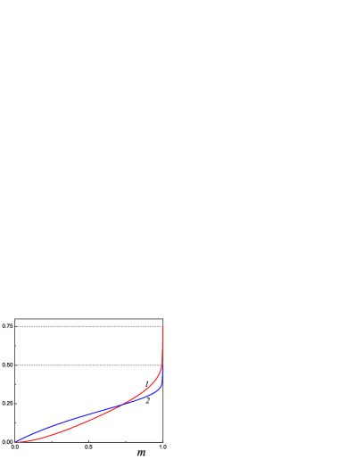
Figure 3: Functions: (1) $f(m)$  (54), (2) $g(m)$  (55).

The free energy per a particle:

$$\begin{array}[]{ccc}\displaystyle{\psi(m)\equiv\frac{\delta F_{W}(m)}{N}=e(m)-Ts(m)=2\,T_{p}g(m)\tau D^{2}+\frac{4}{9}T_{p}(1+\tau)\big{(}3g(m)-f(m)\big{)}D^{4}.}\end{array}$$ (56)

The free energy (56) can be expressed in terms of one function (54):

$$\begin{array}[]{ccc}\displaystyle{\psi(m)=-T_{p}\frac{\tau^{2}}{(1+\tau)}f(m).}\end{array}$$ (57)

Note that near the temperature of transition to the inhomogeneous state, the entropy (49), (52) and the energy (50), (53) are linear in $\tau$, while the free energy (51), (56), (57) is quadratic. Taking into account that $f(1)=3/4$ and $g(1)=1/2$, formulas (52), (53), (56) transform into formulas (49), (50), (51) for the “kink”.

Formulas (49) – (57) determine the contribution of a specific solution of the nonlinear equation (27) to the entropy, energy and free energy. When finding the total thermodynamic quantities, the contributions of all solutions should be taken into account. The contribution of the solution will be the more significant, the lower the free energy associated with it. According to the general principles of statistical physics, the probability $dw=w(m)dm$ of finding a system in a state with parameter $m$ in the interval $m\div m+dm$ is determined by a “single-particle” distribution function over states $m$: $\displaystyle{w(m;\tau)\sim\exp\!\bigg{(}\!-\frac{\psi(m;\tau)}{T}\bigg{)}=\exp\!\bigg{(}\frac{\tau^{2}}{(1+\tau)^{2}}f(m)\bigg{)}}$. Function $f(m)$ is increasing and reaches its maximum value $f(1)=3/4$ at $m=1$ (Fig. 3, curve 1). With a small deviation from $m=1$, it decreases very quickly from its maximum value as $f(m)\approx f(1)-2\big{/}\ln\!\!\big{[}16/(1-m)\big{]}$. Therefore, it is more convenient to define the distribution function in terms of the difference $\Delta f(m)\equiv f(m)-f(1)$, so that we set

$$\begin{array}[]{ccc}\displaystyle{w(m;\tau)=\frac{1}{Z(\tau)}\exp\!\bigg{(}\frac{\tau^{2}}{(1+\tau)^{2}}\Delta f(m)\bigg{)}.}\end{array}$$ (58)

The statistical integral $Z(\tau)$ is defined by the normalization condition $\int_{0}^{m_{*}(\tau)}\!w(m;\tau)dm=1$:

$$\begin{array}[]{ccc}\displaystyle{Z(\tau)=\int_{0}^{m_{*}(\tau)}\!e^{\frac{\tau^{2}}{(1+\tau)^{2}}\Delta f(m)}dm,}\end{array}$$ (59)

where the integration is carried out over all permissible values of the parameter $m$, which vary from zero to the maximum value $m_{*}$. Since $f(m)$ is an increasing function, then the solutions close to the maximum value $m_{*}$ make the main contribution to the thermodynamic quantities. In the K -phase the solution with the maximum $m_{*}=1$ is the “kink” (39). Taking into account that ${\rm sn}u\approx{\rm th}u$ [10] at $m\rightarrow 1$, in this limit solution (40) goes over to (39). Thus, in the K -phase, where $m_{*}=1$, the main contribution to the thermodynamic quantities is made by the solution in the form of the “kink”. In the W -phase, the maximum value of the parameter $m$ depends on temperature

$$\begin{array}[]{ccc}\displaystyle{m_{*}(\tau)=\frac{1}{\big{(}4D^{2}-1\big{)}}=-\frac{(1+\tau)}{(1+7\tau)}=\frac{T/T_{p}}{6-7\big{(}T/T_{p}\big{)}},}\end{array}$$ (60)

and thermodynamics is determined only by solutions of the form of concentration waves. The temperature dependence of the parameter $m_{*}(\tau)$ (60) is shown in Fig. 4.

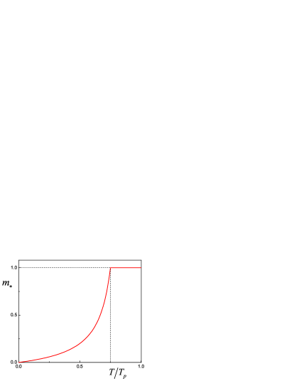
Figure 4: Dependence of the maximum value of the parameter $m\equiv m_{*}(T)$ on temperature.

The form of distribution functions in both inhomogeneous phases is shown in Fig. 5.

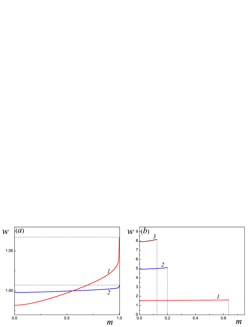
Figure 5: Distribution functions $w(m;\tau)$ at certain temperatures: (a) in the K -phase at (1) $\tau=-0.25$, (2) $\tau=-0.1$; (b) in the W -phase at (1) $\tau=-0.3$, (2) $\tau=-0.5$, (3) $\tau=-0.6$.

The average value of an arbitrary function $\Phi(m)$ is found by the formula

$$\begin{array}[]{ccc}\displaystyle{\big{\langle}\Phi\big{\rangle}=\int_{0}^{m_{*}}\!\Phi(m)\,w(m;\tau)\,dm.}\end{array}$$ (61)

Averaging expressions (52), (53) and (57), we obtain the average values of entropy, energy and free energy, which are expressed through the average values of functions (54), (55):

$$\begin{array}[]{ccc}\displaystyle{\langle s\rangle=-2\Big{[}\langle g\rangle D^{2}+\frac{2}{9}\langle f\rangle D^{4}\Big{]},}\end{array}$$ (62)

$$\begin{array}[]{ccc}\displaystyle{\langle e\rangle=T_{p}\Big{[}-2\langle g\rangle D^{2}+\frac{4}{9}(1+\tau)\big{(}3\langle g\rangle-2\langle f\rangle\big{)}D^{4}\Big{]},}\end{array}$$ (63)

$$\begin{array}[]{ccc}\displaystyle{\langle\psi\rangle=-T_{p}\frac{\tau^{2}}{(1+\tau)}\langle f\rangle.}\end{array}$$ (64)

The heat capacity per a particle at constant volume follows from formula (62) for the entropy:

$$\begin{array}[]{ccc}\displaystyle{\frac{C_{V}}{N}=T\frac{d\langle s\rangle}{dT}=-\bigg{\{}2D^{2}\langle g\rangle\bigg{[}T\frac{d\ln\langle g\rangle}{dT}+\frac{1}{\tau}\bigg{]}+\frac{4}{9}D^{4}\langle f\rangle\bigg{[}T\frac{d\ln\langle f\rangle}{dT}+\frac{2}{\tau}\bigg{]}\bigg{\}}.}\end{array}$$ (65)

From formulas (62) – (64) it also follows that there holds the identity $\langle\psi\rangle=\langle e\rangle-T\langle s\rangle$. Note that in work [1] the entropy was defined through the average of the logarithm of the one-particle distribution function, as is customary in the theory of rarefied gases [11]. However, in this case the direct calculation of the entropy, which is based on the use of formula (9) for the free energy, shows that the entropy of the inhomogeneous state is not reduced to the average of the logarithm of the distribution function. Therefore, in respect to the calculation of the entropy and heat capacity, we corrected the results of work [1]. The results of a new calculation of the temperature dependences of the entropy and heat capacity by the formulas (62), (65) are shown in Fig. 6.

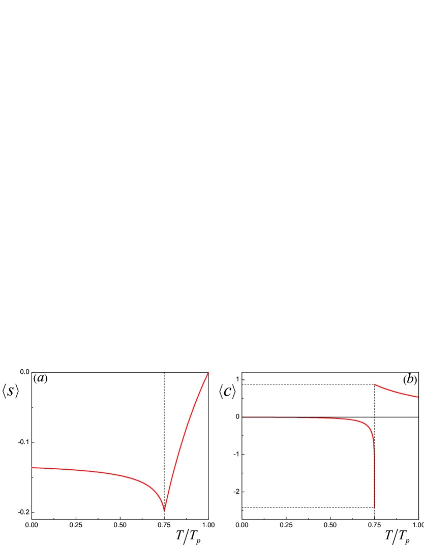
Figure 6: Temperature dependencies of the inhomogeneity contribution: (a) to entropy, (b) to heat capacity.

VI Transitions between phases. Heat capacity.

Above the temperature $T_{p}$ the solution is in the homogeneous state (H -phase). In the temperature range $T_{1}<T<T_{p}$, there arises the K -phase in which the states both in the form of the “kink” (39) and in the form of the concentration waves (40) are possible. For the “kink” the parameter $m\equiv m_{*}=1$, and for the waves in this phase it varies in the interval $0\leq m<1$, but the main contribution to thermodynamics is made by the “kink”. Consider the transition from the homogeneous state to the K -phase. Near the transition temperature at $|\tau|\ll 1$, the entropy (62) is $\langle s\rangle\approx 3\langle g\rangle_{0}\tau$, where $\langle g\rangle_{0}=\int_{0}^{1}\!g(m)dm$. Therefore, during the transition from the H -phase to the K -phase the heat capacity undergoes a jump

$$\begin{array}[]{ccc}\displaystyle{\frac{\Delta C}{N}=3\langle g\rangle_{0}\approx 0.533.}\end{array}$$ (66)

Note that the jump in the isochoric heat capacity per a particle (66) is a number which does not depend on the parameters of the system and thermodynamic quantities.

In the temperature range $0<T<T_{1}$ , there is the W -phase in which there are possible states only in the form of the concentration waves (40). In this phase the parameter changes in the interval $0\leq m\leq m_{*}$, where $m_{*}$ is defined by formula (60) (Fig. 4). With a decrease in temperature at $T_{1}\big{/}T_{p}=3/4$ or $\tau_{1}=-1/4$, a phase transition from the K - to the W -phase occurs. Near the temperature of transition between these inhomogeneous phases the entropy can be represented as

$$\begin{array}[]{ccc}\displaystyle{\langle s\rangle=\langle s\rangle_{1}+\zeta_{1}\Delta\tau+\zeta_{2}\Delta m_{*},}\end{array}$$ (67)

where $\Delta\tau=\tau-\tau_{1}$,

$$\begin{array}[]{ccc}\displaystyle{\Delta m_{*}(\tau)=1-m_{*}(\tau)=\left\{\begin{array}[]{l}\,\,\,\,0,\qquad\Delta\tau>0,\vspace{2mm}\\ \displaystyle{\frac{32}{3}}\Delta\tau,\,\,\,\,\Delta\tau<0,\end{array}\!\right.}\end{array}$$ (68)

and also

$$\begin{array}[]{ccc}\displaystyle{\langle s\rangle_{1}=-\Big{(}\frac{7}{12}+\langle\Delta g\rangle_{1}+\frac{1}{9}\langle\Delta f\rangle_{1}\Big{)},}\end{array}$$ (69)

$$\begin{array}[]{ccc}\displaystyle{\zeta_{1}=\frac{32}{27}\Big{[}\Big{(}\big{\langle}\Delta f\Delta g\big{\rangle}_{1}-\langle\Delta f\rangle_{1}\langle\Delta g\rangle_{1}\Big{)}+\frac{1}{9}\Big{(}\big{\langle}(\Delta f)^{2}\big{\rangle}_{1}-\langle\Delta f\rangle_{1}^{2}\Big{)}\Big{]}+\frac{16}{3}\Big{[}\frac{2}{3}+\langle\Delta g\rangle_{1}+\frac{2}{9}\langle\Delta f\rangle_{1}\Big{]},}\end{array}$$ (70)

$$\begin{array}[]{ccc}\displaystyle{\zeta_{2}=w(1;\tau_{1})\Big{(}\langle\Delta g\rangle_{1}+\frac{1}{9}\langle\Delta f\rangle_{1}\Big{)}.}\end{array}$$ (71)

Here $\langle\ldots\rangle_{1}$ means averaging with the distribution function $w(m;\tau_{1})$, and $w(1;\tau_{1})=1/Z(\tau_{1})$. From formulas (67) – (71) it follows that during the transition between the inhomogeneous phases the heat capacity undergoes a negative jump (Fig. 6b)

$$\begin{array}[]{ccc}\displaystyle{\frac{\Delta C}{N}=\frac{\big{(}C_{W}-C_{K}\big{)}}{N}=8\zeta_{2}.}\end{array}$$ (72)

The qualitative difference between the results of this calculation in comparison with the previous one [1] is that the transition from the homogeneous state to the K -phase is the second-order phase transition with a jump in the heat capacity. The transition from the high-temperature inhomogeneous K -phase to the low-temperature inhomogeneous W -phase remains, just as in [1], the second-order transition, but with a negative jump in the heat capacity (Fig. 6b).

Let us also consider the behavior of the entropy and heat capacity in the low-temperature limit $T\rightarrow 0$, when $1+\tau\equiv\alpha\ll 1$. Since in this case $m_{*}\ll 1$, then there hold the approximations $f(m)\approx 9m^{2}/8$, $g(m)\approx 0.5\big{(}m-7m^{2}/8\big{)}$. In view of this we find

$$\begin{array}[]{ccc}\displaystyle{\langle s\rangle=s_{0}-s_{0}^{\prime}\frac{T}{T_{p}},}\end{array}$$ (73)

$$\begin{array}[]{ccc}\displaystyle{\frac{C}{N}=-s_{0}^{\prime}\frac{T}{T_{p}},}\end{array}$$ (74)

where

$$\begin{array}[]{ccc}\displaystyle{s_{0}=-\sqrt{2}\rho_{1}-\rho_{2},\qquad s_{0}^{\prime}=\frac{\sqrt{2}\,e^{1\!/32}}{192\,r_{0}(0)}\Big{[}\big{(}1-4\sqrt{2}\rho_{1}\big{)}+\Big{(}\frac{1}{8}-4\rho_{2}\Big{)}\Big{]},}\end{array}$$ (75)

and here $\rho_{n}=r_{n}(0)/r_{0}(0)$, $r_{n}(0)=\int_{0}^{\sqrt{2}/8}e^{y^{2}}y^{n}\,dy$. Thus, the contribution of inhomogeneity effects to the heat capacity at $T\rightarrow 0$ tends to zero in proportion to temperature, and the entropy tends to the constant value $s_{0}$ linearly with temperature. Note that this does not contradict the basic principles of thermodynamics, since under the used classical description the entropy is determined up to a constant value, and a physical meaning has a difference of entropies. To estimate the temperature range in which the influence of quantum effects can be neglected, we use the requirement of smallness of the thermal de Broglie wavelength $\Lambda_{B}\sim\hbar\big{/}\sqrt{MT}$ ($M$ is the reduced mass of particles in a solution) in comparison with the period of the concentration wave. Since the wave period tends to the correlation length $\xi_{0}=\sqrt{K/a_{0}}$ in the low-temperature limit, we have the condition $\xi_{0}\gg\Lambda_{B}$. From it there follows the limitation on temperature values at which the classical description is permissible:

$$\begin{array}[]{ccc}\displaystyle{T\gg\frac{\hbar^{2}}{M\xi_{0}^{2}}.}\end{array}$$ (76)

For $M\sim 10^{-22}$ g and $\xi_{0}\sim 10^{-8}$ cm, it gives $T\gg 1$ K.

VII Conclusion

In this work on the basis of a theoretical approach to the description of a binary solution, previously proposed by the authors in [1], the role of the cubic in concentration term in the expansion of the free energy is studied and a refined calculation of the contribution of inhomogeneity to thermodynamic quantities is given. It is shown that taking into account the cubic term contributes to the stability of the spatially homogeneous state of the solution. In the considered model of an isotropic medium, the phase transition to the inhomogeneous state proves to be possible only at half the concentration. At other concentrations solutions of the equation for the concentration in the form of concentration waves also exist, but they do not satisfy the matching condition which follows from the requirement of conservation of the number of particles, and therefore are not realized. Note, however, that our calculations were carried out under the assumption that the total density is constant. Accounting for the inhomogeneity of the total density should probably lead to an expansion of the range of concentrations at which the transition to the inhomogeneous phase is possible.

Using the introduced distribution function of inhomogeneous states, the contribution of inhomogeneity to the entropy and heat capacity is calculated. This calculation refines and corrects the corresponding calculation of the previous work [1]. It is shown that during the transition from the homogeneous state to the inhomogeneous state and the transition between two inhomogeneous phases the heat capacity undergoes a jump, so that these transitions are second-order phase transitions. When approaching zero temperature, the contribution to the heat capacity from inhomogeneity decreases linearly with decreasing temperature. An estimate is given of the temperature range in which the classical description is acceptable.

References

(1)
Yu.M. Poluektov, A.A. Soroka, Transition of a binary solution into
an inhomogeneous phase, Phase Transition 95 (4), 267 (2022). doi:10.1080/01411594.2022.2041015; arXiv:2109.02404 [cond-mat.stat-mech]
(2)
J.W. Cahn, J.E. Hilliard, Free energy of a nonuniform system. I.
Interfacial free energy, J. Chem. Phys. 28, 258 (1958).
doi:10.1063/1.1744102
(3)
J.W. Cahn, J.E. Hilliard, Free energy of a nonuniform system. II.
Thermodynamic basis, J. Chem. Phys. 30, 1121 (1959).
doi:10.1063/1.1730145
(4)
J.W. Cahn, J.E. Hilliard, Free energy of a nonuniform system. III.
Nucleation in a two-component incompressible fluid, J. Chem. Phys. 31, 688 (1959). doi:10.1063/1.1730447
(5)
M. Hillert, A solid-solution model for inhomogeneous systems, Acta
Metallurgica 9, 525 (1961).
doi:10.1016/0001-6160(61)90155-9
(6)
A.G. Khachaturian, Theory of phase transformations and structure of
solid solutions, Nauka, Moscow, 384 p. (1974).
(8)
T. Muto, Yu. Takagi, The theory of order-disorder transitions in
alloys, Solid State Physics 1, 193 (1955).
doi:10.1016/S0081-1947(08)60679-7
(9)
I.S. Gradshteyn and I.M. Ryzhik, Tables of integrals, series and
products, Fizmatgiz, Moscow, 1100 p. (1963).
(10)
M. Abramowitz, I. Stegun (Editors), Handbook of mathematical
functions, National Bureau of Standards Applied mathematics Series
55, 1046p. (1964).
(11)
J.H. Ferziger, H.G. Kaper, Mathematical theory of transport
processes in gases, North-Holland, Amsterdam, 579 p. (1972).