No-regret Algorithms for Fair Resource Allocation

Abstract

We consider a fair resource allocation problem in the no-regret setting against an unrestricted adversary. The objective is to allocate resources equitably among several agents in an online fashion so that the difference of the aggregate $\alpha$-fair utilities of the agents between an optimal static clairvoyant allocation and that of the online policy grows sub-linearly with time. The problem is challenging due to the non-additive nature of the $\alpha$-fairness function. Previously, it was shown that no online policy can exist for this problem with a sublinear standard regret. In this paper, we propose an efficient online resource allocation policy, called Online Proportional Fair (OPF), that achieves $c_{\alpha}$-approximate sublinear regret with the approximation factor $c_{\alpha}=(1-\alpha)^{-(1-\alpha)}\leq 1.445,$ for $0\leq\alpha<1$. The upper bound to the $c_{\alpha}$-regret for this problem exhibits a surprising phase transition phenomenon. The regret bound changes from a power-law to a constant at the critical exponent $\alpha=\nicefrac{{1}}{{2}}.$ As a corollary, our result also resolves an open problem raised by Even-Dar et al. (2009) on designing an efficient no-regret policy for the online job scheduling problem in certain parameter regimes. The proof of our results introduces new algorithmic and analytical techniques, including greedy estimation of the future gradients for non-additive global reward functions and bootstrapping adaptive regret bounds, which may be of independent interest.

1 Introduction

The notion of algorithmic fairness refers to learning algorithms that guarantee fair predictions even when subjected to adversarially-biased training data (Dwork et al., 2012). In addition to efficiency, fairness has become a major criterion for designing and deploying large-scale learning algorithms that affect a diverse user base. Since the training data could be highly skewed in practice, it is essential to make minimal assumptions about the data-generating process and design provably robust fair learning policies. Guaranteeing fairness becomes even more challenging in the online learning set-up as there is no distinction between the training and test data, and no assumption is made on the input data sequence. As an example, consider an online recruitment campaign where a learning algorithm decides the target group (identified by, say, the tuple (race, gender, age)) to which an ad for a job vacancy is to be displayed. Suppose a revenue-maximizing recommendation algorithm concludes from past data that more revenue is generated by showing the ad to Group A compared to Group B. In that case, it will eventually end up showing that ad exclusively to Group A while discriminating against Group B users of a potential job opportunity (Hao, 2019). One of the overarching goals of this paper is to design efficient online learning policies that provably mitigate this algorithmic bias while maintaining efficiency irrespective of the past data seen so far (refer to Example 2.2 for a relevant model for the above example considered in this paper).

Towards this goal, we consider a generic online fair resource allocation problem called NOFRA (No-Regret Fair Resource Allocation). In this problem, a fixed set of resources needs to be equitably shared among $m$ agents over multiple rounds. Note that fairness is a complex, multidimensional, and essentially subjective concept. Several quantitative metrics have been introduced in the literature for quantifying the degree of fairness in resource allocation, including $\alpha$-fairness (Lan et al., 2010), proportional fairness (Kelly, 1997; Mo and Walrand, 2000), max-min fairness (Radunovic and Le Boudec, 2007; Nace and Pióro, 2008), and Jain’s fairness index (Jain et al., 1984). In this paper, we consider the problem of maximizing the $\alpha$-fairness function, in which the utility of each agent when allocated $R$ units grows as $R^{1-\alpha}$. The parameter $\alpha$ is restricted to the interval $[0,1).$ This same range of $\alpha$ has been studied earlier in a game-theoretic set up by Altman et al. (2010).

On the hardness of the NOFRA problem:

In the standard online learning setting, the cumulative reward accrued over a given time horizon is taken to be the sum of the rewards obtained at each round (Hazan, 2019). In contrast, the objective of the NOFRA problem is to maximize the global $\alpha$-fairness function, which is equal to the sum of cumulative rewards of each agent raised to the power $1-\alpha,0\leq\alpha<1$. Because of the power-law non-linearity, the objective function of the NOFRA problem is non-additive with respect to time. Note that the non-additivity of the objective function is essential to induce fairness in sequential allocations by incorporating the diminishing return property. However, this renders the NOFRA problem fundamentally different from standard online learning problems. In particular, Theorem 2 proves a non-trivial lower bound to the approximation ratio achievable by any online learning policy for this problem. This lower bound does not hold in classic settings with additive rewards. Although some specific problems with non-additive reward functions have been previously studied in the online learning literature (Si Salem et al., 2022; Even-Dar et al., 2009; Rakhlin et al., 2011), in the following, we explain why the NOFRA problem is fundamentally different from the existing studies.

Related work:

In a closely-related paper, Si Salem et al. (2022) considered the problem of designing fair online resource allocation policies. The authors showed that it is impossible to design a no-regret policy without restricting the set of admissible adversarial demand sequences. Given this negative result, the authors proposed a no-regret policy using a primal-dual framework under the assumption of a restricted adversary, which exhibits an essentially i.i.d. random-like $o(T)$ fluctuation. In contrast, we design a robust policy with an approximate sublinear regret without restricting the adversary. Due to the weaker assumption, our policy and its analysis are also very different from that of Si Salem et al. (2022). Wang et al. (2022) considered an online resource allocation problem where the objective is to guarantee a sublinear regret for the allocation efficiency and a sublinear minimum guarantee violation penalty. The authors proposed an online policy that achieves this goal by using a weighted $\alpha$-fair allocation on each round while sequentially tuning the weights and the exponents of the $\alpha$-fairness function. Although they use round-wise $\alpha$-fair allocation as a tool, their objective is not to optimize the $\alpha$-fairness of the cumulative allocation, which is the focus of our paper. even2009online considered optimizing a global concave objective function in the no-regret setup, under the further assumption that the optimal reward is convex. They presented an approachability-based policy in this setting and also proved the impossibility of achieving zero regret when the convexity condition is violated. In our case of the $\alpha$-fairness function for $0\leq\alpha<1$, although the objective function is concave, we show that the optimal static offline reward function fails to be convex (see Appendix 7.7). Hence, their policy does not apply to the NOFRA problem. The paper by rakhlin2011online considered the problem of no-regret learnability for a wide class of non-additive global functions. However, their results also do not apply to our setting as our problem is not no-regret learnable (see Theorem 2). Several prior works exist that design no-regret policies for specific non-additive functions. As an example, blum1997line; fine-paging used online learning techniques for solving the online paging and the Metrical Task System problem, which contains states. The fairness problem has also been extensively studied in the stochastic multi-armed bandit setting (narahari-fair; joseph2016fairness; li2019combinatorial).

Our contributions:

We show that despite its non-additive structure, the NOFRA problem can be approximately reduced to an instance of an online linear optimization problem with a greedily defined sequence of reward vectors. In particular, we make the following contributions:

• In Algorithm 1, we present an efficient online resource allocation policy, called Online Proportional Fair (OPF), that approximately maximizes the aggregate $\alpha$-fairness function of the agents in the sense of standard regret. We show that the above policy achieves $(1-\alpha)^{-(1-\alpha)}\leq 1.445$-approximate sublinear regret (Theorem 1). To the best of our knowledge, OPF is the first online policy that approximately maximizes the $\alpha$-fairness for any adversarial sequence.

• In Theorem 2, we establish a lower bound to the approximation factor $c_{\alpha}$ achievable by any online learning policy for the $\alpha$-fair reward function. Our lower bound improves upon the best-known lower bound for this problem.

• On the algorithmic side, we introduce a new class of online policies for optimizing non-additive global reward functions by greedily estimating the future gradients and using these estimated gradients within an online gradient ascent policy with adaptive step sizes. The resulting algorithm is simple and intuitive: we have weights on each user that decay as the user’s cumulative reward increases. We show that the greedy estimation is sufficient for obtaining a constant-factor approximate sublinear regret for the $\alpha$-fair reward function.

• On the analytical side, we introduce a new proof technique that simultaneously controls the magnitude of the gradients and the adaptive regret bound under the above policy. This technique applies to problems with memory or states where the future gradients depend on past actions.

2 Problem Formulation

In this section, we give a general formulation of the NOFRA problem. In Section 2.1, we give examples of three concrete resource allocation problems that fit into this general framework.

Let the term agents denote entities among which a limited resource is to be fairly divided. Assume that the resource allocated to the $i$^th agent on the $t$^th round is represented by an $N$-dimensional non-negative Euclidean vector $y_{i}(t)$, where $N$ is an arbitrary number. On every round $t$, the $i$^th agent requests an $N$-dimensional non-negative demand (or, reward) vector $x_{i}(t)$. The demand vectors are revealed to an online allocation policy $\pi$ at the end of each round. We make no assumption on the regularity of the demand vector sequence, which could be adversarially chosen (c.f., si2022enabling). Before the $N\times m$ dimensional aggregate demand matrix $\bm{x}(t)\equiv\big{(}x_{1}(t),x_{2}(t),\ldots,x_{m}(t)\big{)}$ for round $t$ is revealed, the online resource allocation policy $\pi$ chooses a non-negative $N\times m$ dimensional allocation matrix $\bm{y}(t)=\big{(}y_{1}(t),y_{2}(t),\ldots,y_{m}(t)\big{)}$ from the set of all feasible allocations $\Delta$. The set of all feasible allocations is assumed to be convex (see Remark 2 below). The reward accrued by the agent $i$ on round $t$ is given by the inner-product $\langle x_{i}(t),y_{i}(t)\rangle,$ which, without any loss of generality, is assumed to be upper-bounded by one. The total cumulative reward accrued by agent $i$ agent at the end of round $t$ is given by

$$R_{i}(t+1)=R_{i}(t)+\langle x_{i}(t),y_{i}(t)\rangle,~{}\forall i,t,$$ (1)

where $R_{i}(0)=0,\forall i.$ By iterating the above recursion, the cumulative reward $R_{i}(t)$ can be alternatively expressed as follows:

$$R_{i}(t)=\sum_{\tau=1}^{t-1}\langle x_{i}(\tau),y_{i}(\tau)\rangle.$$ (2)

We make two mild technical assumptions on the structure of the demand and allocation vectors.

Assumption 1.

$\delta\leq||x_{i}(t)||_{1}\leq 1,\forall i,t,$ for some constant $\delta>0.$

Assumption 2.

Let $\bm{1}_{N\times m}$ denote the $N\times m$ all-$1$ matrix. Then $\mu\bm{1}_{N\times m}\in\Delta$ for some constant $\mu>0.$

The above assumptions imply that it is possible to ensure a non-zero reward for all agents on all rounds. This property will be exploited in the proofs of our regret bounds (see Eq. (25)).

The utility of any user for a cumulative reward of $R$ is given by the concave $\alpha$-fair utility function $\phi:\mathbb{R}_{+}\to\mathbb{R}_{+},$ defined as follows:

$$\phi(R)=\phi_{\alpha}(R)\equiv\frac{R^{1-\alpha}}{1-\alpha},~{}~{}R\geq 0,$$ (3)

for some constant $0\leq\alpha<1$. The fairness parameter $\alpha$ induces a trade-off between the desired efficiency and fairness by incorporating a notion of diminishing return property in the global objective function. The static offline optimal allocation with larger $\alpha$ leads to more equitable cumulative rewards (bertsimas2012efficiency). Setting $\alpha=0$ reduces the problem to the “unfair” online linear optimization problem. Our objective is to design an online resource allocation policy $\pi\equiv\{\bm{y}(t)\}_{t\geq 1}$ that minimizes the regret for maximizing the aggregate utilities of all users compared to any fixed offline resource allocation strategy $\bm{y}^{*}\in\Delta.$ To be precise, assume that the offline, fixed resource allocation $\bm{y}^{*}$ yields a cumulative reward of $\bm{R}^{*}(T)$ at the end of round $T\geq 1.$ Then, our objective is to design a resource allocation policy which minimizes the $c$-approximate regret (which we refer to as $c$-regret for short) defined as:

$$\textrm{Regret}_{T}(c)\equiv\sum_{i=1}^{m}\phi(R_{i}^{*}(T))-c\sum_{i=1}^{m}\phi(R_{i}(T)),$$ (4)

for some small constant $c\geq 1.$ In the case of standard regret ($c=1$), we drop the argument in the parenthesis. Note that, unlike the standard online convex optimization problem, in the NOFRA problem, the reward function is global, in the sense that it is non-separable across time (even2009online). For this reason, it is necessary to consider the $c$-regret with $c>1$, rather than the standard regret (i.e., with $c=1$). This will become clear from Theorem 2, where we prove an explicit lower bound to the approximation factor achievable by any online policy for the global $\alpha$-fair reward function. This lower bound implies a concrete lower bound on the achievable $c$. Our lower bound improves upon (si2022enabling, Theorem 1), where it was shown that no online policy can achieve a sublinear standard regret for the NOFRA problem under an unrestricted adversary.

Remark 1: When $\alpha>1,$ the offline benchmark $\phi(R_{i}^{*}(T))$ itself becomes $O(1),\forall i.$ Hence, in this regime, a sublinear regret bound (4) becomes vacuous. Consequently, we restrict the fairness parameter $\alpha$ to the interval $[0,1).$

Remark 2: Apart from Section 4, we assume that the set of feasible allocations $\Delta$ is convex and thus that there are no integrality constraints on the allocation, i.e., the components of the allocation matrix $\bm{y}(t)$ are allowed to be fractional. However, in many combinatorial resource allocation problems, such as shared caching (Example 2.1), the allocation vector is required to be integral. In this case, the feasible action set $\Delta$ is naturally defined to be the convex hull of the integral actions. In Section 4, we consider the integrality constraints on the allocation vector and derive a randomized integral allocation policy with a sublinear regret bound as a corollary of our results for the relaxed problem.

2.1 Examples

The statement of NOFRA is fairly general and by suitably choosing the reward and allocation vectors, many resource allocation problems can be reduced to NOFRA. In this section, we highlight three such problems: fair allocation in online shared caching, online job scheduling, and online matching.

Example 2.1 (Online Shared Caching (SIGMETRICS20)).

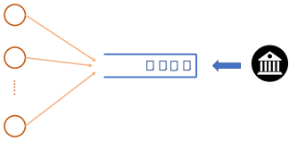
Figure 1: Online shared caching problem

In the Online Shared Caching problem with a single shared cache, $m$ users are connected to a single cache of capacity $k$ (see Figure 1 for a schematic). At each round, each user requests a file from a library of size $N.$ The file request sequence may be adversarial. At the beginning of each round $t$, an online caching policy prefetches at most $k$ files on the cache, denoted by the vector $y(t)$ such that

$$\sum_{i=1}^{N}y_{i}(t)=k,~{}~{}0\leq y_{i}(t)\leq 1~{},\forall i\in[m].$$ (5)

The set of all feasible caching configurations is denoted by $\Delta^{N}_{k}.$ Immediately after the prefetching at round $t$, each user $i$ reveals its file request, represented by the one-hot encoded demand vector $x_{i}(t)$, $1\leq i\leq m$. A special case of the above caching model for a single user ($m=1$) has been investigated in previous work (SIGMETRICS20; mhaisen2022optimistic; ITW22).

Let $R_{i}(t)$ denote the cumulative (fractional) hits obtained by the $i$^th user up to round $t\geq 1$. Clearly,

$$R_{i}(T)=\sum_{t=1}^{T}\langle x_{i}(t),y(t)\rangle,~{}~{}1\leq i\leq m,$$ (6)

The online shared caching problem can be easily reduced to an instance of the NOFRA problem by taking the demand matrix to be $\bm{x}(t)=\big{(}x_{1}(t),x_{2}(t),\ldots,x_{m}(t)\big{)}.$ Since the allocation vector $y(t)$ is common to all users, the allocation matrix can be taken to be $\bm{y}(t)=\big{(}y(t),y(t),\ldots,y(t)\big{)}.$ It can be observed that Assumption 2 holds in this case with $\mu=k/N$ by noting that $\frac{k}{N}\bm{1}_{N}\in\Delta^{N}_{k}.$

Example 2.2 (Online Job Scheduling (even2009online)).

In this problem, there are $m$ machines, which play the role of agents. A single job arrives at each round. The reward accrued by assigning the incoming job at round $t$ to the $i$^th machine is given by $x_{i}(t)$ where $x_{i}(t)\in[\delta,1],\forall i\in[m],$ where $\delta>0$ is a small positive constant. Before the rewards for round $t$ are revealed, an online allocation policy selects a probability distribution $\bm{y}_{t}$ on $m$ machines such that

$$\sum_{i=1}^{m}y_{i}(t)=1,~{}y_{i}(t)\geq 0,\forall i\in[m].$$

The policy allocates a fraction $y_{i}(t)$ of the job to the $i$^th machine $\forall i\in[m]$. As a result, the $i$^th machine accrues a reward of $x_{i}(t)y_{i}(t)$ on round $t.$ Hence, the cumulative reward accrued by the $i$^th machine in a time-horizon of length $T$ is given by:

$$R_{i}(T)=\sum_{t=1}^{T}x_{i}(t)y_{i}(t),~{}\forall i\in[m].$$

The objective of the online fair job scheduling problem is to design an online allocation policy that achieves a sublinear regret with respect to the $\alpha$-fairness of the cumulative rewards defined in (4). From the above description, it is immediately clear that this problem is a special case of the general NOFRA problem. The Online job scheduling problem occurs in many practical contexts, e.g., in the targeted ad-campaigning problem discussed in the introduction, the ads can be modelled as jobs and different groups of users can be modelled as machines.

Example 2.3 (Online Matching).

Consider an $m\times m$ bipartite graph where the vertices on the left denote the agents and the vertices on the right denote the resources. On every round, each agent can be matched with one resource only, where we allow fractional matchings. The $m\times 1$ demand vector of the agent $i$ on round $t$ is denoted by $x_{i}(t).$ The $j$^th component of the demand vector $x_{i}(t)$ denotes the potential reward accrued by the $i$^th agent had it been completely matched with the $j$^th resource on round $t$. Let the binary action variable $y_{ij}(t)\in[0,1]$ denote the amount by which the agent $i$ is matched with resource $j$ on round $t$. Hence, the reward accrued by the agent $i$ on time $t$ is given by $\langle x_{i}(t),y_{i}(t)\rangle.$ Let $\Delta$ denote the convex hull of all matchings. It is well known that $\Delta$ can be succinctly represented by the set of all $m\times m$ doubly stochastic matrices, a.k.a. the Birkhoff polytope (ziegler2012lectures)). In other words, in the OFM problem, the set of all feasible actions $\Delta$ consists of all $m\times m$ matrices $\big{(}y_{ij}\big{)}_{i,j}$ satisfying the following constraints :

$$\sum_{i=1}^{m}y_{ij}=1,~{}\forall j,~{}~{}\sum_{j=1}^{m}y_{ij}=1,~{}\forall i,~{}~{}0\leq y_{ij}\leq 1,~{}\forall i,j.$$ (7)

Let the variable $R_{i}(t)$ denote the cumulative rewards accried by the $i$^th agent up to round $t$. Clearly,

$$R_{i}(t+1)=R_{i}(t)+\langle x_{i}(t),y_{i}(t)\rangle,R_{i}(0)=0,~{}~{}1\leq i\leq m,$$ (8)

It can be verified that Assumption 2 holds in this problem with $\mu=m^{-1}$ by noting that $m^{-1}\bm{1}_{m\times m}\in\Delta.$ The objective of the Online Fair Matching (OFM) problem is to design an online matching policy that minimizes the $c$-Regret (4). Figure 2 illustrates a special case of the problem for binary-valued demands. From the above formulation, it can be immediately seen that the Online Matching problem is an instance of the NOFRA problem. Furthermore, it also generalizes the online scheduling problem described in Example 2.2.

The online matching problem arises in numerous practical settings. For example, in the problem of online Ad Allocation, there are $m$ different advertisers whose ads need to be placed in $m$ different display slots on a webpage. Each slot can accommodate only one ad. On round $t$, a new user arrives and presents a reward vector $\bm{x}_{i}(t)$ for each advertiser. For example, the component $x_{ij}(t)$ could denote potential revenue accrued by the advertiser if the ad $i$ is placed on the $j$^th slot on round $t$. The objective of the allocation policy is to match the ads to the slots on each round so that the total earned revenue is fairly distributed among the advertisers. Similar problems arise in designing recommendation systems for crowdsourcing or online dating websites (tu2014online), fair channel assignment in wireless networks (ALTMAN2010338).

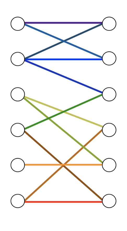
A Bipartite graph $\mathcal{G}$

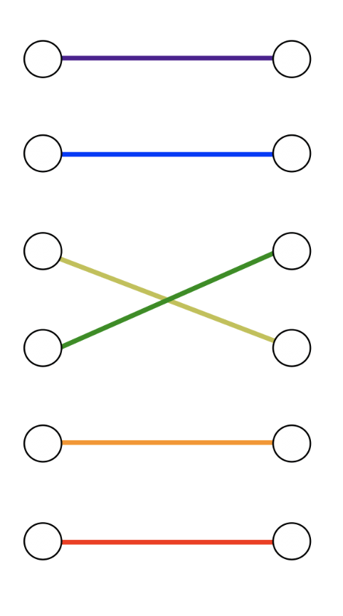
A Matching in $\mathcal{G}$

Figure 2: Illustrating the Online Fair Matching (OFM) problem for zero-one demands. The existence of an edge denotes unit demand, and likewise, the absence of any edge implies zero demand.

3 Designing an approximately-no-regret policy for NOFRA

In view of the difficulty outlined in Section 1, the design and analysis of the Online Proportional Fair (OPF) policy consists of two parts. First, in Lemma 1, we show that by greedily estimating the terminal gradient with the current gradients at each round, the standard regret of the NOFRA problem can be upper bounded by the $(1-\alpha)^{-(1-\alpha)}$-approximate static regret of a surrogate online linear optimization problem with a policy-dependent gradient sequence. Finally, we use the online gradient ascent policy with adaptive step sizes to solve the surrogate problem while simultaneously controlling the magnitude of the gradients. The following section details our technique.

3.1 Reducing the NOFRA problem to an Online Linear Optimization Problem with policy-dependent subgradients

Since the fairness function $\phi:\mathbb{R}_{+}\to\mathbb{R}_{+}$ is concave, we have that for any $x,y\geq 0:$

$$\phi(x)-\phi(y)\leq\phi^{\prime}(y)(x-y).$$ (9)

Let $\beta\geq 1$ be some constant to be determined later. Taking $x=R_{i}^{*}(T)$ and $y=\beta R_{i}(T)$ in the above inequality, we have

$$\phi(R_{i}^{*}(T))-\beta^{1-\alpha}\phi(R_{i}(T)) \stackrel{{\scriptstyle(a)}}{{=}} \phi(R_{i}^{*}(T))-\phi(\beta R_{i}(T)),$$ (10)

$$\stackrel{{\scriptstyle(b)}}{{\leq}} \phi^{\prime}(\beta R_{i}(T))(R_{i}^{*}(T)-\beta R_{i}(T))$$

$$\stackrel{{\scriptstyle(c)}}{{=}} \beta^{-\alpha}\phi^{\prime}(R_{i}(T))\sum_{t=1}^{T}\langle x_{i}(t),y_{i}^{*}-\beta y_{i}(t)\rangle.$$

where in (a), we have used the positive homogeneity property of the fairness function $\phi(\beta x)=\beta^{1-\alpha}\phi(x),$ in (b), we have used the concavity of the fairness function $\phi(\cdot)$ from Eqn. (9), and, finally, in (c), we have used the definition of cumulative rewards (2) and the homogeneity of the function $\phi(\cdot)$ to conclude that $\phi^{\prime}(\beta x)=\beta^{-\alpha}\phi^{\prime}(x).$

Summing up the bound (10) over all agents $i\in[m]$, we obtain the following upper bound to the $\beta^{1-\alpha}$-Regret of any online policy for the NOFRA problem:

$$\textrm{Regret}_{T}(\beta^{1-\alpha})\leq\beta^{-\alpha}\sum_{t=1}^{T}\bigg{(}\sum_{i}\langle\phi^{\prime}(R_{i}(T))x_{i}(t),y_{i}^{*}-\beta y_{i}(t)\rangle\bigg{)}.$$ (11)

It is critical to note that each of the quantities $\phi^{\prime}(R_{i}(T))$ depends on the entire sequence of past actions $\{y_{t}\}_{t=1}^{T}.$ Hence, (11) is not the standard regret as the terminal value of $\phi^{\prime}(R_{i}(T))$ is not known to the online policy when it takes its actions. More importantly, the value of the coefficient $\phi^{\prime}(R_{i}(T))$ depends on the future actions and requests through (1), and hence, it is impossible to know the value of this coefficient in an online fashion. To get around this fundamental difficulty, we now consider a surrogate regret-minimization problem by replacing the term $\phi^{\prime}(R_{i}(T))$ by its causal version $\phi^{\prime}(R_{i}(t))$ on round $t$. In other words, we now seek to design an online learning policy $\pi$ that minimizes the regret of the following surrogate online linear optimization problem:

$$\hat{\textrm{Regret}_{T}}\equiv\sum_{t=1}^{T}\bigg{(}\sum_{i}\langle\phi^{\prime}(R_{i}(t))x_{i}(t),y_{i}^{*}-y_{i}(t)\rangle\bigg{)}.$$ (12)

To recapitulate the information structure, recall that the cumulative reward vector $\bm{R}(t)$ is known, but the current request vector $\bm{x}(t)$ is unknown to the online learner before it makes a decision $y_{t}$ on the $t$^th round. We now establish the following central result that relates the bound (11) to the regret bound (12) of the online linear optimization problem.

Lemma 1.

Consider any arbitrary online resource allocation policy and assume that the utility function of each user is given by the $\alpha$-fair utility function (3). Then, we have

$$\textrm{Regret}_{T}(c_{\alpha})\leq(1-\alpha)^{\alpha}\hat{\textrm{Regret}_{T}},$$ (13)

where $c_{\alpha}\equiv(1-\alpha)^{-(1-\alpha)}\leq e^{1/e}<1.445.$

Proof outline

As discussed above, the surrogate problem greedily replaces the non-causal terminal gradient $\phi^{\prime}(R_{i}(T))$ in Eqn. (11) by the current gradient $\phi^{\prime}(R_{i}(t)),\forall i$ on round $t$. The proof of Lemma 1 revolves around showing that this transformation can be done by incurring only a small penalty factor to the overall regret bound. For proving this result, we split the regret expression (11) into the difference between two terms - term $(A)$ corresponding to the cumulative reward accrued by the benchmark static allocation ($\bm{y}^{*}$), and term $(B)$ corresponding to the reward accrued by the online policy. Next, we compare these two terms separately with the corresponding terms $(A^{\prime})$ and $(B^{\prime})$ in the regret expression for the surrogate online linear optimization problem (12). By exploiting the non-decreasing nature of the cumulative rewards, we first show that $(A)\leq(A^{\prime})$ (see Eqn. (16)). Next, by using form of the $\alpha$-fair utility function, we show that $(B^{\prime})\leq(1-\alpha)^{-1}(B)$ under the action of any policy (see Eqn. (17)). Lemma 1 then follows by combining the above two results. See Appendix 7.3 for the proof of Lemma 1.

3.2 Online Learning Policy for the Surrogate Problem and its Regret Analysis

Algorithm 1 The Online Proportional Fair (OPF) Policy

1:Input: Fairness parameter $0\leq\alpha<1$, Demand/Reward vectors from the agents $\{\bm{x}(t)\}_{t=1}^{T},$ Euclidean projection oracle $\Pi_{\Delta}(\cdot)$ onto the feasible set $\Delta,$ an upper-bound $D$ to the Euclidean diameter of the feasible set.

2:Output: Online resource allocation decisions $\{y_{t}\}_{t=1}^{T}$

3:$R_{i}\leftarrow 1,\forall i\in[m],\bm{y}\leftarrow\mu\mathds{1}_{N\times m},S\leftarrow 0$ $\triangleright$ Initialization

4:for each round $t=2:T$: do

5:     $g_{i}\leftarrow\frac{x_{i}(t-1)}{R_{i}^{\alpha}},\forall i\in[m]$ $\triangleright$ Computing the gradient components for each agents

6:     $g\leftarrow(g_{1},g_{2},\ldots,g_{m})$ $\triangleright$ Computing the full gradient

7:     $S\leftarrow S+||g||_{2}^{2},$ $\triangleright$ Accumulating the norm of the gradients

8:     $y\leftarrow\Pi_{\Delta}\big{(}y+\frac{D}{2\sqrt{S}}g\big{)}$ $\triangleright$ Updating the inclusion probabilities using OGA

9:     [Optional] Sample a randomized integral allocation $Y$ s.t. $\mathbb{E}[Y]=y.$

10:     The agents reveal their demand/ reward vectors $\{x_{i}(t)\}_{i\in[m]}$ for the current round.

11:     $R_{i}\leftarrow R_{i}+\langle x_{i}(t),y_{i}(t)\rangle,~{}\forall i\in[m].$ $\triangleright$ Updating cumulative rewards

12:end for each

Having established that the $c$-regret of the original problem is upper bounded by the regret of the surrogate learning problem, we now proceed to upper bound the regret of the surrogate problem under the action of a no-regret learner. In the sequel, we use the projected Online Gradient Ascent (OGA) with adaptive step sizes (orabona2019modern, Algorithm 2.2) for designing a no-regret policy for the surrogate problem. We call the resulting online learning policy Online Proportional Fair (OPF). The pseudocode of the OPF policy is given in Algorithm 2.

The Online Proportional Fair policy (OPF):

At the end of each round, each user $i$ computes its gradient component $g_{i}$ by dividing its current demand vector $x_{i}(t-1)$ with its current cumulative reward $R_{i}(t)$ raised to the power $\alpha$ (line 5 of Algorithm 1). This formalizes the intuition that a user with a larger current cumulative reward has a smaller gradient component. In line 8, we take a projected gradient ascent step, where the projection operation constitutes the main computational bottleneck. In practice, the projection can often be computed efficiently using variants of the Frank-Wolfe algorithm while given access to an efficient LP oracle. With additional structure, the OPF policy can be simplified further with a more efficient projection. For example, we give a simplified implementation for the online shared caching problem in Appendix 7.5 by exploiting the fact that the action vector $y(t)$ is the same for all users, i.e., $y_{1}(t)=y_{2}(t)=\ldots=y_{m}(t)\equiv y(t),\forall t.$ Step 9 is an optional sampling step which is executed only if an integral allocation is required. For pedagogical reasons, we will skip Step 9 in this section and discuss it later in Section 4. Finally, the cumulative rewards of all users are updated in step 11. The following lemma gives an upper bound to the regret of the OPF policy for the surrogate problem.

Lemma 2.

The Online Proportional Fair policy, described in Algorithm 1 achieves the following standard regret bound for the surrogate problem (12) for the $\alpha$-fair utility function:

$$\hat{\textrm{Regret}}_{T}=\begin{cases}O(T^{1/2-\alpha}),~{}~{}\textrm{if}~{}~{}0<\alpha<\nicefrac{{1}}{{2}},\\ O(\sqrt{\log T}),~{}~{}\textrm{if}~{}~{}\alpha=\nicefrac{{1}}{{2}}\\ O(1),~{}~{}\textrm{if}~{}~{}\nicefrac{{1}}{{2}}<\alpha<1.\end{cases}$$

Furthermore, under this policy, the cumulative rewards of each user increases linearly with time, i.e., $R_{i}(T)=\Omega(T),\forall i,T$.

Proof outline:

One of the major challenges in the regret analysis of the surrogate problem (12) is that the coefficients of the gradients $\{\phi^{\prime}(R_{i}(t)),i\in[m]\}$ on round $t$ depends on the past actions $\{\bm{y}(\tau)\}_{\tau=1}^{t}$ of the policy itself. Since the regret bound of any online linear optimization problem scales with the norm of the gradients, we now need to simultaneously control the regret and the norm of the gradients generated by the online policy. Surprisingly, the proof of Theorem 7.4 shows that the proposed online gradient ascent policy with adaptive step sizes not only provides a sublinear regret but it also keeps the gradients small, which in turn helps keep the regret small. In fact, these two goals are well-aligned and our proof precisely exploits the reinforcing nature of these two objectives via a new Bootstrapping technique. See Appendix 7.4 for the proof of Lemma 2.

Finally, combining Lemma 1 and Lemma 2, we obtain the main result of this paper.

Theorem 1 ((Regret bound of the OPF policy)).

The Online Proportional Fair (OPF) policy, described in Algorithm 1, achieves the following approximate regret bound for the NOFRA problem (4):

$$\textrm{Regret}_{T}(c_{\alpha})=(1-\alpha)^{\alpha}\begin{cases}O(T^{1/2-\alpha})~{}~{}\textrm{if}~{}~{}0<\alpha<\nicefrac{{1}}{{2}},\\ O(\sqrt{\log T})~{}~{}\textrm{if}~{}~{}\alpha=\nicefrac{{1}}{{2}}\\ O(1)~{}~{}\textrm{if}~{}~{}\nicefrac{{1}}{{2}}<\alpha<1,\end{cases}$$ (14)

where $c_{\alpha}\equiv(1-\alpha)^{-(1-\alpha)}$.

Remarks:

1. For the job scheduling problem in the reward maximization setting, even2009online showed that if the cumulative reward is concave and the offline optimal reward is convex, then their proposed (albeit complex) approachability-based recursive policy achieves zero-regret. In Section 7 of the same paper, the authors posed an open problem of attaining a relaxed goal when the above sufficient condition is violated. In Appendix 7.7, we show that for the $\alpha$-fair utility function (3), the offline optimal cumulative reward is non-convex in the regime $0<\alpha<1$. Hence, Theorem 1 gives a resolution to the above open problem by exhibiting a simple online policy with a sublinear approximate regret when the given sufficient condition is violated. Furthermore, the computational complexity of our policy is linear in the number of machines $m,$ which is way better than their approachability-based policy whose complexity scales exponentially in $m$.

2. Observe that the regret bound given by Theorem 2 always remains non-vacuous, irrespective of the value of the fairness parameter $\alpha$ and the sequence of adversarial reward vectors. This follows from the fact that irrespective of the demand vectors, by choosing the constant action $y=\mu\mathds{1},$ each user can achieve a cumulative reward of $\mu\delta T.$ Hence, the optimal offline value of the $\alpha$-fair utility function $\Omega(T^{1-\alpha}).$ On the other hand, the OPF policy achieves a regret bound of $O(T^{\nicefrac{{1}}{{2}}-\alpha}),$ (Theorem 1) that is always dominated by the optimal static offline objective.

3. In the special case of $\alpha=0,$ the NOFRA problem corresponds to the cumulative reward maximization problem for all users. Hence, Theorem 2 recovers the well-known $O(\sqrt{T})$ standard regret bound obtained by SIGMETRICS20 in the context of online caching.

The following converse result gives a universal lower bound to the approximation factor $c$ for which it is possible to design an online policy with a sublinear $c$-regret.

Theorem 2 ((Lower bound to the approximation factor)).

Consider the online shared caching problem for the $\alpha$-fair reward function with $m=2$ users. Then for any online policy with a sublinear $c_{\alpha}$-regret, we must have

$$c_{\alpha}\geq\max_{0\leq\eta\leq\nicefrac{{1}}{{2}}}\frac{{\eta}^{1-\alpha}+{(1-\eta)}^{1-\alpha}}{{(1-\eta/2)}^{1-\alpha}+{({\eta}/{2})}^{1-\alpha}}>1,~{}~{}0<\alpha<1.$$

A numerical comparison between the upper and lower bounds on the approximation factor is shown in Figure 3. See Appendix 7.8 for the proof of Theorem 2.

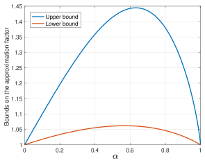
Figure 3: Comparison between the upper and lower bounds of the approximation ratio

4 High-probability regret bound for randomized integral allocations

Theorem 2 establishes $c_{\alpha}\equiv(1-\alpha)^{-(1-\alpha)}$-regret guarantee for the Online Proportional Fair (OPF) policy for fractional allocations where the set of admissible actions $\Delta$ is the convex hull of integral allocations. In the following, we show that a sub-linear $c_{\alpha}$-regret guarantee holds with high probability when randomized integral actions are chosen according to the optional step (9) in the OPF policy. Recall that for integral allocation, on each round $t$ we independently sample an integral allocation $Y_{t}\in\{0,1\}^{mN},$ that matches with the fractional allocation $y_{t}$ in expectation, i.e., $\mathbb{E}[Y_{t}]=y_{t}$ where $y_{t}$ is the fractional allocation vector recommended by the OPF policy. A fractional allocation vector $y_{t}$ in the convex hull of integral allocations can be turned to a randomized integral allocation by expressing $y_{t}$ as a convex combination of integral allocations and then randomly sampling one of the integral allocations with appropriate probabilities. As Appendix 7.6 shows, for many problems with structure, such a decomposition can be efficiently computed.

Regret analysis:

By appealing to (cesa2006prediction, Lemma 4.1), it is enough to consider an oblivious adversary that fixes the sequence of demand vectors $\{\bm{x}(t)\}_{t\geq 1}$ before the game commences. Let the random variable $\mathsf{R}_{i}(T)$ denote the random cumulative reward obtained by the $i$^th user under the randomized integral allocation policy and the deterministic variable $R_{i}(T)$ is defined as in Eqn. (2). By construction, we have $\mathbb{E}[\mathsf{R}_{i}(T)]=R_{i}(T).$ Furthermore, since $\mathsf{R}_{i}(T)$ is the sum of $T$ independent random variables, each of magnitude at most one, from the standard Hoeffding’s inequality, we have

$$\mathbb{P}(|\mathsf{R}_{i}(T)-R_{i}(T)|\geq\lambda)\leq\exp(-2\lambda^{2}/T),\forall i\in[m].$$

Hence, with probability at least $1-\texttt{poly}(1/T),$ the aggregate $\alpha$-fair utility (3) accrued by the randomized policy can be lower bounded as:

$$(1-\alpha)^{-1}\sum_{i}\mathsf{R}^{1-\alpha}_{i}(T) \geq (1-\alpha)^{-1}\sum_{i}\bigg{(}R_{i}(T)-O(\sqrt{T\log T})\bigg{)}^{1-\alpha}$$ (15)

$$\stackrel{{\scriptstyle(a)}}{{\geq}} (1-\alpha)^{-1}\sum_{i}R_{i}^{1-\alpha}(T)-O\big{(}(T\log T)^{\frac{1-\alpha}{2}}\big{)},$$

where in inequality (a), we have used the fact that $(x+y)^{1-\alpha}\leq x^{1-\alpha}+y^{1-\alpha},\forall 0\leq\alpha\leq 1,x,y\geq 0.$ Combining the above with the approximate regret bound in Theorem 1, and taking the dominant term, we conclude that the $c_{\alpha}$-regret for the randomized integral allocation policy is upper-bounded by $O\big{(}(T\log T)^{\frac{1-\alpha}{2}}\big{)}$ w.h.p. for all $0\leq\alpha\leq 1.$ Unfortunately, unlike Theorem 1, the integral allocation policy incurs a non-trivial (but sublinear) $c_{\alpha}$-regret for the entire range of the fairness parameter $0\leq\alpha<1.$

5 Conclusion and open problems

In this paper, we propose an efficient online resource allocation policy, called Online Proportional Fair (OPF), that achieves a $c_{\alpha}$-approximate sublinear regret bound for the $\alpha$-fairness objective, where $c_{\alpha}\equiv(1-\alpha)^{-(1-\alpha)}\leq 1.445,$ for $0<\alpha<1.$ Our main technical contribution is to show that the non-additive $\alpha$-fairness function can be efficiently learned by greedily estimating the terminal gradients. An important follow-up problem is to investigate the extent to which the algorithmic and analytical methodologies introduced in this paper can be generalized. Specifically, it would be interesting to see if a similar online policy can be designed for the online scheduling problem in the regime $\alpha>1.$ Note that, for the online scheduling problem, only a recursive approachability-based policy is known in the literature, whose complexity scales exponentially with the number of machines (even2009online). Another related problem is to design an optimistic version of the proposed OPF policy that offers an improved regret bound by efficiently incorporating hints regarding the future demand sequence (mhaisen2022optimistic; bhaskara2020online). Furthermore, reducing the gap between the upper and lower bounds of the approximation factor in Figure 3 would be interesting. Finally, designing an online resource allocation policy with a small dynamic regret would give a more fine-grained regret bound depending on the regularity of the demand/reward sequence.

6 Acknowledgement

This work was supported by a US-India NSF-DST collaborative grant coordinated by IDEAS-Technology Innovation Hub (TIH) at the Indian Statistical Institute, Kolkata. C. Musco was also partially supported by an Adobe Research grant.

7 Appendix

7.1 Proof of the inequality $\phi^{\prime}(R_{i}(t))(R_{i}(t+1)-R_{i}(t))\leq\int_{R_{i}(t)-1}^{R_{i}(t+1)-1}\phi^{\prime}(R)dR$

We use the fact that $\phi^{\prime}(\cdot)$ is a non-increasing function and $R_{i}(t+1)-R_{i}(t)\leq 1.$ The following diagram is self-explanatory.

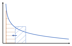
Figure 4: Graphical proof of the upper bound

7.2 Upper bound on the diameter of the admissible sets

Lemma 3.

For the online shared caching problem the diameter of the admissible action set can be bounded as follows:

$$\textrm{Diam}(\Delta^{N}_{k})\leq\sqrt{2k}.$$

Proof.

Let $x,y\in\Delta^{N}_{k}.$ We have

$$||x-y||_{2}^{2}=\sum_{i=1}^{N}(x_{i}-y_{i})^{2}=\sum_{i=1}^{N}|x_{i}-y_{i}||x_{i}-y_{i}|\stackrel{{\scriptstyle(a)}}{{\leq}}\sum_{i=1}^{N}|x_{i}-y_{i}|\stackrel{{\scriptstyle(b)}}{{\leq}}\sum_{i=1}^{N}|x_{i}|+\sum_{i=1}^{N}|y_{i}|\stackrel{{\scriptstyle(c)}}{{=}}2k,$$

where, in (a), we have used the fact that $0\leq x_{i},y_{i}\leq 1,$ in (b), we have used triangle inequality, and in (c), we have used the fact that the sum of the components of each feasible vector is $k$. ∎

Lemma 4.

For the online matching problem, the diameter of the admissible action set can be bounded as follows:

$$\textrm{Diam}(\Delta)\leq\sqrt{2m}.$$

Let $x,y\in\Delta,$ where $\Delta$ is the feasible set for the OFM problem. We have

$$||x-y||_{2}^{2}=\sum_{i,j}(x_{ij}-y_{ij})^{2}\leq\sum_{i,j}|x_{ij}-y_{ij}|\leq\sum_{ij}x_{ij}+\sum_{ij}y_{ij}\leq 2m,$$

where the inequalities follow from similar arguments as in the proof of the previous lemma.

7.3 Proof of Lemma 1

Proof.

The expression for $\textrm{Regret}_{T}(\beta^{1-\alpha})$ from Eqn. (11) can be split into two terms as follows:

$$\textrm{Regret}_{T}(\beta^{1-\alpha})=\beta^{-\alpha}\big{[}\underbrace{\sum_{i}\phi^{\prime}(R_{i}(T))\sum_{t=1}^{T}\langle x_{i}(t),y_{i}^{*}\rangle}_{\textrm{{\color[rgb]{0,0,1}$(A)$}}}-\beta\underbrace{\sum_{i}\phi^{\prime}(R_{i}(T))\sum_{t=1}^{T}\langle x_{i}(t),y_{i}(t)\rangle}_{\textrm{{\color[rgb]{0,0,1}$(B)$}}}\big{]}.$$

Also denote the corresponding terms in the regret expression (12) for the surrogate learning problem by $(A^{\prime})$ and $(B^{\prime})$. We will now separately bound each of the above two terms in terms of the corresponding terms in the regret expression (12) for the surrogate learning problem.

Proving $(A)\leq(A^{\prime})$

Recall that the utility function $\phi(\cdot)$ is concave. Hence, its derivative is non-decreasing in its argument. Furthermore, under the action of any policy, the cumulative reward $R_{i}(\cdot)$ is non-decreasing for each user $i\in[m].$ Thus, we have $\phi^{\prime}(R_{i}(t))\geq\phi^{\prime}(R_{i}(T))$ for all $t\in[T],i\in[m].$ Hence,

$$(A)\leq\sum_{t=1}^{T}\langle\sum_{i}\phi^{\prime}(R_{i}(t))x_{i}(t),y_{i}^{*}\rangle\leq(A^{\prime}).$$ (16)

Proving $(B^{\prime})\leq(1-\alpha)^{-1}(B)$

We have

$$(B)^{\prime} = \sum_{i}\sum_{t=1}^{T}\phi^{\prime}(R_{i}(t))\langle x_{i}(t),y_{i}(t)\rangle$$ (17)

$$= \sum_{i}\sum_{t=1}^{T}\phi^{\prime}(R_{i}(t))\big{(}R_{i}(t+1)-R_{i}(t)\big{)}$$

$$\stackrel{{\scriptstyle(a)}}{{\leq}} \sum_{i}\int_{0}^{R_{i}(T)}\phi^{\prime}(R)dR$$

$$= \sum_{i}\phi(R_{i}(T))$$

$$\stackrel{{\scriptstyle(b)}}{{=}} (1-\alpha)^{-1}\sum_{i}\phi^{\prime}(R_{i}(T))R_{i}(T)$$

$$\stackrel{{\scriptstyle(c)}}{{=}} (1-\alpha)^{-1}\sum_{i}\phi^{\prime}(R_{i}(T))\sum_{t=1}^{T}\langle x_{i}(t),y_{i}(t)\rangle$$

$$= (1-\alpha)^{-1}(B),$$

where, in (a), we have used the fact that $\phi^{\prime}(\cdot)$ is non-increasing and $R_{i}(t+1)-R_{i}(t)=\langle x_{i}(t),y_{i}(t)\leq 1$ (see Figure 7.1 in the Appendix for a geometric visualization), in (b), we have used the explicit form of the $\alpha$-fair utility function to substitute $x\phi^{\prime}(x)=(1-\alpha)\phi(x)$, and in (c), we have used (2). Combining (16) and (17) and choosing $\beta=(1-\alpha)^{-1},$ we conclude that

$$\textrm{Regret}_{T}((1-\alpha)^{-(1-\alpha)})\leq(1-\alpha)^{\alpha}\hat{\textrm{Regret}_{T}}.$$

∎

7.4 Proof of Lemma 2

Proof.

We will be using the following adaptive regret bound for the online gradient descent policy with an appropriate adaptive step sizes sequence. We will see that the norm of the gradients diminishes at a steady rate under the action of the OPF policy. Hence, the data-dependent regret bound plays a central role for a tight regret analysis of the OPF policy.

Theorem 3 ((Theorem 4.14 of orabona2019modern)).

Let $\Delta\subset\mathbb{R}^{d}$ be a convex set with with diameter $D.$ Let us consider a sequence of linear reward functions with gradients $\{\bm{g}_{t}\}_{t\geq 1}.$ Run the Online Gradient Ascent policy with step sizes $\eta_{t}=\frac{D}{\sqrt{2\sum_{\tau=1}^{t}||\bm{g}_{\tau}||_{2}^{2}}},1\leq t\leq T.$ Then the standard regret under the OGA policy can be upper-bounded as follows:

$$\textrm{Regret}_{T}\leq D\sqrt{2\sum_{t=1}^{T}||\bm{g}_{t}||_{2}^{2}}.$$ (18)

Note that, the gradient component $g_{i}$ corresponding to the $i$^th user for the surrogate problem (12) on round $t$ is given by the vector $g_{i}(t)=\phi^{\prime}(R_{i}(t))x_{i}(t).$ Using the above data-dependent static regret bound (18), the regret achieved by the OGA policy for the surrogate problem for any round $T\geq 1$ can be upper-bounded as follows:

$$\hat{\textrm{Regret}}_{T}=O\bigg{(}\sqrt{\sum_{t=1}^{T}\sum_{i}\phi^{\prime}(R_{i}(t))^{2}}\bigg{)}=O\bigg{(}\sqrt{\sum_{t=1}^{T}\sum_{i}\frac{1}{R_{i}(t)^{2\alpha}}}\bigg{)},$$ (19)

where we have used the fact that the demand vectors at each round are bounded.

Clearly, the regret bound (19) depends on the sequence of the cumulative rewards $\{\bm{R}(t)\}_{t\geq 1}$, which is implicitly controlled by the past actions of the online policy itself. By the definition of regret, for any fixed allocation $y^{*}\in\Delta^{N}_{k},$ we have for any time step $T$:

$$\sum_{t=1}^{T}\sum_{i}\langle\phi^{\prime}(R_{i}(t))x_{i}(t),y_{i}(t)\rangle\geq\sum_{t=1}^{T}\sum_{i}\langle\phi^{\prime}(R_{i}(t))x_{i}(t),y_{i}^{*}\rangle-\hat{\textrm{Regret}}_{T},$$ (20)

where $\hat{\textrm{Regret}}_{T}$ denotes the worst-case cumulative regret of the adaptive OGD policy up to time $T$. Since the cumulative reward of each user is monotonically non-decreasing, we have:

$$R_{i}(T)\geq 1,\forall i,\forall T.$$ (21)

This can easily be ensured by an appropriate initialization using Assumptions 1 and 2.

Substituting this bound to the regret bound in (19), we obtain our first (loose) upper-bound for the regret of the fair allocation problem (12):

$$\hat{\textrm{Regret}}_{T}=O(\sqrt{T}).$$ (22)

Note that this bound might be too loose as the offline benchmark itself could be smaller in magnitude than this regret bound. A closer inspection reveals the root cause for this looseness - the cumulative reward lower bound (21) is too loose for our purpose, as cumulative rewards grow steadily with time, depending on the online policy. We now strengthen the above upper-bound using a novel bootstrapping method, that simultaneously tightens the lower bound for the cumulative rewards (21) and, consequently, improves the regret upper bound (19).

Using the fact that $\langle x_{i}(t),y_{i}(t)\rangle=R_{i}(t+1)-R_{i}(t),$ and following the same steps as (17), we have

$$\sum_{i}\sum_{t=1}^{T}\phi^{\prime}(R_{i}(t))\langle x_{i}(t),y_{i}(t)\rangle\leq\sum_{i}\phi(R_{i}(T)).$$ (23)

Furthermore, lower bounding $\phi^{\prime}(R_{i}(t))$ by $\phi^{\prime}(R_{i}(T)),$ we have

$$\sum_{t=1}^{T}\sum_{i}\langle\phi^{\prime}(R_{i}(t))x_{i}(t),y_{i}^{*}\rangle\geq\sum_{i}\phi^{\prime}(R_{i}(T))R_{i}^{*}(T),$$ (24)

where $R_{i}^{*}(T)\equiv\sum_{t=1}^{T}\langle x_{i}(t),y_{i}^{*}\rangle$ is the cumulative reward accrued by a fixed allocation $y^{*}\in\Delta$ up to time $T.$ Using Assumptions 1 and 2 and choosing $y_{i}^{*}=\mu\mathds{1}_{N},$ we have $R_{i}^{*}(T)\geq\mu\delta T,\forall i.$ Hence, combining (23), (24), and (20), we have

$$\sum_{i}\phi(R_{i}(T))\geq\mu\delta T\sum_{i}\phi^{\prime}(R_{i}(T))-\hat{\textrm{Regret}}_{T}.$$ (25)

Since $0<R_{i}(T)\leq T,\forall i,$ and $\phi(\cdot)$ is monotone non-decreasing, for any user $i\in[m]$, the above inequality yields:

$$\frac{m}{(1-\alpha)T^{\alpha}}\geq\frac{\mu\delta}{R_{i}^{\alpha}(T)}-\frac{\hat{\textrm{Regret}}_{T}}{T}.$$

i.e.,

$$R_{i}^{\alpha}(T)\geq\mu\delta\bigg{(}\frac{\hat{\textrm{Regret}}_{T}}{T}+\frac{m}{1-\alpha}T^{-\alpha}\bigg{)}^{-1}=\Omega(T^{\min(1/2,\alpha)}),\forall i\in[m],$$ (26)

where we have used our previous upper bound (22) on the regret. Eqn. (26) is our key equation for carrying out the bootstrapping process as it lower bounds the minimum cumulative reward of users in terms of the worst-case regret. Now we consider two cases:

Figure 5: Illustrating the new Bootstrapping technique used in the proof of Lemma 2

Case-I: $0\leq\alpha\leq\nicefrac{{1}}{{2}}$

In this case, we immediately have $R_{i}(T)=\Omega(T),\forall i,T.$ Substituting this bound on (19), we have

$$\hat{\textrm{Regret}}_{T}=\begin{cases}O(\sqrt{\log T})~{}~{}\textrm{if}~{}~{}\alpha=1/2\\ O(T^{1/2-\alpha})~{}~{}\textrm{if}~{}~{}0<\alpha<1/2.\end{cases}$$

Case-II: $\nicefrac{{1}}{{2}}<\alpha<1$

In this case, using the bound (26), we have $R_{i}(T)=\Omega(T^{1/2\alpha}),\forall i,T.$ Using the regret bound (19), the regret can be bounded as

$$\hat{\textrm{Regret}}_{T}=O(\sqrt{\sum_{t=1}^{T}\frac{1}{t}})=O(\sqrt{\log T}).$$

Substituting this bound again in (26), we have $R_{i}(T)\geq\Omega(T).$ This, in turn, yields the following regret bound:

$$\hat{\textrm{Regret}}_{T}=O\big{(}\sqrt{\sum_{t=1}^{T}\frac{1}{t^{2\alpha}}}\big{)}=O(1).$$

∎

7.5 Simplified Pseudocode for the Online Proportional Fair Policy for the Caching Problem

Algorithm 2 Online Proportional Fair Caching (OPFC)

1:Input: Fairness parameter $0\leq\alpha<1.$ Online file request sequence $\{x_{i}(t)\}_{t=1}^{T}$ from user $i,i\in[m],$ Euclidean projection oracle $\Pi_{\Delta^{N}_{k}}(\cdot)$ onto the feasible convex set $\Delta^{N}_{k}.$

2:Output: Sequence of file inclusion probabilities $\{y_{t}\}_{t=1}^{T}$ and samples from this distribution

3:$R_{i}\leftarrow 1,\forall i\in[m],\bm{y}\leftarrow\frac{k}{N}\mathds{1}_{N},S\leftarrow 0.$ $\triangleright$ Initialization

4:for each round $t=2:T$: do

5:     $g\leftarrow\sum_{i=1}^{m}\frac{x_{i}(t-1)}{R_{i}^{\alpha}}$ $\triangleright$ Computing the gradient

6:     $S\leftarrow S+||g||_{2}^{2},$ $\triangleright$ Accumulating the norm of the gradients

7:     $y\leftarrow\Pi_{\Delta^{N}_{k}}\big{(}y+\frac{k}{\sqrt{S}}g\big{)}$ $\triangleright$ Updating the inclusion probabilities using OGA

8:     The users reveal their latest file requests $\{x_{i}(t),i\in[m]\}.$

9:     $R_{i}\leftarrow R_{i}+\langle x_{i}(t),y\rangle,~{}\forall i\in[m].$ $\triangleright$ Updating cumulative hits $\triangleright$ Sample a subset of $k$ files by invoking Algorithm 3

10:end for each

7.6 Efficiently sampling an integral allocation from a mixed allocation in the convex hull

1. Online shared caching:

For the online shared caching problem, the admissible set $\Delta$ is given by Eq. (5). Clearly, incidence vectors of all $k$-sets, containing $k$ 1’s and $N-k$ zeros, belong to $\Delta.$ Furthermore, given any vector in $\bm{y}\in\Delta,$ a randomized integral allocation can be sampled in linear time using Madow’s sampling scheme, described in Algorithm 3, which yields the vector $\bm{y}$ in expectation.

Algorithm 3 Madow-Sample ($p$)

1:Input: A universe $[N]$ of size $N$, the cardinality of the sampled set $k$, and a marginal inclusion probability vector $p\in\Delta^{N}_{k}.$

2:Output: A random $k$-set $S$ with $|S|=k$ such that, $\mathbb{P}(i\in S)=p_{i},\forall i\in[N]$

3:Define $\Pi_{0}=0$, and $\Pi_{i}=\Pi_{i-1}+p_{i},\forall 1\leq i\leq N.$

4:Sample a uniformly distributed random variable $U$ from the interval $[0,1].$

5:$S\leftarrow\emptyset$

6:for each $i\leftarrow 0$ to $k-1$ do

7:     Select the element $j$ if $\Pi_{j-1}\leq U+i<\Pi_{j}.$

8:end for each

9:return $S$

2. Online job scheduling:

In the online job scheduling problem the admissible action set $\Delta$ is given by the $N$-simplex. Given any point on the $N$-simplex, it is trivial to randomly sample a coordinate using a single uniform random variable.

3. Online matching:

In the online matching problem, the admissible action set $\Delta$ is given by the Birkhoff polytope (7). Given any point $\bm{y}$ in the Birkhoff polytope, it can be efficiently decomposed as a convex combination of a small number of matchings using the Birkhoff-von-Neumann (BvN) decomposition algorithm (valls2021birkhoff). Using the coefficients of the decomposition, a matching can be randomly sampled that exactly matches the point $\bm{y}$ in expectation.

7.7 Non-Convexity of the optimal offline benchmark for the online job scheduling problem

Consider the job scheduling problem in the reward maximization setting as described in Example 2.2. Clearly, the $\alpha$-fairness metric accumulated by the online policy is concave in the regime $0\leq\alpha\leq 1.$ However, the following proposition shows that the offline static benchmark for this problem is non-convex for the $\alpha$-fair utility function in the regime $0<\alpha<1.$

Proposition 1.

The offline optimal $\alpha$-fair reward function for the job scheduling problem is non-convex for $0<\alpha<1.$

Proof.

Let the probability distribution $\bm{y}^{*}$ be an optimal static offline allocation vector for the reward sequence $\{\bm{x}_{t}\}_{t\geq 1}.$ Also, let $R_{T}(i)\equiv\sum_{t}x_{i}(t)$ be the cumulative reward observed by the $i$^th machine, $1\leq i\leq m$. Then the optimal allocation $\bm{y}^{*}$ maximizes the following objective:

$$(1-\alpha)^{-1}\sum_{i}(y_{i}R_{T}(i))^{1-\alpha}.$$ (27)

s.t. the constraints $\sum_{i}y_{i}=1,\bm{y}\geq\bm{0}.$ Since $0<\alpha<1,$ the objective function is strongly concave and the optimal solution $\bm{y}^{*}$ is unique. Using the standard Hölder’s inequality with the conjugate norms $p=\nicefrac{{1}}{{1-\alpha}},q=\nicefrac{{1}}{{\alpha}},$ we can upper bound the objective (27) as

$$(1-\alpha)^{-1}\sum_{i=1}^{m}(y_{i}R_{T}(i))^{1-\alpha} \leq (1-\alpha)^{-1}(\sum_{i}y_{i})^{1-\alpha}(\sum_{i}R_{T}(i)^{\frac{1-\alpha}{\alpha}})^{\alpha}$$ (28)

$$= (1-\alpha)^{-1}(\sum_{i}R_{T}(i)^{\frac{1-\alpha}{\alpha}})^{\alpha},$$

where we have used the constraint $\sum_{i}y_{i}=1$ in the last equality. The upper-bound is achieved by the following distribution

$$y^{*}_{i}=\frac{R_{i}^{\frac{1-\alpha}{\alpha}}}{\sum_{i}R_{i}^{\frac{1-\alpha}{\alpha}}},~{}\forall i\in[m].$$ (29)

Hence, the optimal offline reward (27) is given by

$$\mathcal{R}^{*}=(1-\alpha)^{-1}(\sum_{i}R_{T}(i)^{\frac{1-\alpha}{\alpha}})^{\alpha}.$$ (30)

To show that $\mathcal{R}^{*}$ is non-convex in the cumulative reward vector $\bm{R}_{T}$ in the regime $0<\alpha<1,$ consider the case of two users. Letting $x=R_{T}(1),y=R_{T}(2)$ and ignoring the positive pre-factor, the function under consideration is given as follows:

$$f(x,y)=(x^{\frac{1-\alpha}{\alpha}}+y^{\frac{1-\alpha}{\alpha}})^{\alpha}.$$ (31)

Recall that a function is convex if and only if the determinants of all leading principal minors of its Hessian matrix are non-negative. A straightforward computation yields the following expression for the determinant of the Hessian of the function $f(x,y):$

$$\textrm{det}(\nabla^{2}f(x,y))=(2\alpha-1)\frac{(\alpha-1)^{2}x^{1/\alpha-1}y^{1/\alpha-1}(x^{1/\alpha-1}+y^{1/\alpha-1})^{2\alpha}}{(yx^{1/\alpha}+xy^{1/\alpha})^{2}}.$$

Clearly, the determinant becomes strictly negative in the regime $0<\alpha<\frac{1}{2}.$ This shows that the function (31) is non-convex for $0<\alpha<\frac{1}{2}$. On the other hand, we have

$$\frac{\partial^{2}f(x,y)}{\partial x^{2}}=(\alpha-1)\frac{yx^{1/\alpha-2}(x^{1/\alpha-1}+y^{1/\alpha-1})^{\alpha}(\alpha^{2}yx^{1/\alpha}+2\alpha xy^{1/\alpha}-xy^{1/\alpha})}{\alpha(yx^{1/\alpha}+xy^{1/\alpha})^{2}}.$$

In particular, at the point $(1,1)$ the above second partial derivative evaluates to be

$$\frac{\partial^{2}f(x,y)}{\partial x^{2}}|_{(x,y)=(1,1)}=-\frac{2^{\alpha-2}(1-\alpha)}{\alpha}(\alpha^{2}+2\alpha-1),$$

which is strictly negative for $\sqrt{2}-1<\alpha<1.$ Taking the above two results together, we conclude that the offline optimal reward function (31) is non-convex for $0<\alpha<1.$ ∎

7.8 Proof of Theorem 2 (lower bounding the approximation factor)

Consider the following instance of the online shared caching problem with $m=2$ users and a cache of unit capacity. Assume that size ($N$) of the library is sufficiently large. Let the total length of the request sequence be $T$ rounds and let $\eta\in[0,1]$ be some constant fraction to be fixed later. Consider two different file request sequence:

• Instance 1: For the first $\eta T$ rounds, user 1 always requests file 1 and user 2 always requests file 2. For the next $(1-\eta)T$ rounds, user 1 always requests file 2 and user 2 requests a file chosen uniformly at random from the library.

• Instance 2: For the first $\eta T$ rounds, as in Instance $1$, user 1 always requests file 1 and user 2 always requests file 2. However, for the next $(1-\eta)T$ rounds, user 1 requests a random file chosen uniformly at random from the library and user 2 always requests file 1.

We now lower bound the approximation factor achievable by any online policy for the above two request sequences.

Optimal static offline policy: It is easy to see that the optimal offline strategy is to cache file $2$ for all $T$ rounds. Hence, the total $\alpha$-fairness objective accrued by the static offline policy is

$$\textsf{Offline $\alpha$-fairness}=(1-\alpha)^{-1}T^{1-\alpha}\big{[}\eta^{1-\alpha}+(1-\eta)^{1-\alpha}\big{]}.$$

Clearly, the same fairness objective is achieved for the second instance by a static policy that always caches file 1.

Online Policy: Suppose that during the first $\eta T$ rounds, the online policy caches file 1 for $\gamma$ fraction of the time and file 2 for $1-\gamma$ fraction of the time. Since the policy is online, the fraction $\gamma$ remains the same for both instances. Clearly, for the next $(1-\eta)T$ time slots, an optimal online policy caches file 2 for instance 1 and file 1 for instance 2. Taking worst among the two instances, any online policy achieves the following fairness objective:

$$\textsf{Online $\alpha$-fairness}=(1-\alpha)^{-1}T^{1-\alpha}\min\big{(}g(\gamma),g(1-\gamma)\big{)},$$

where $g(\gamma)\equiv\big{(}\gamma\eta+(1-\eta)\big{)}^{1-\alpha}+\big{(}(1-\gamma)\eta\big{)}^{1-\alpha}.$ From simple calculus, it follows that the function $g(\gamma)$ is non-increasing for $0\leq\eta\leq\nicefrac{{1}}{{2}},0\leq\alpha<1.$ This implies that the online $\alpha$-fairness is maximized when $\gamma^{*}=\frac{1}{2}$. Hence, the $\alpha$-fairness metric achieved by any online policy for the worst of the above two instances is upper bounded by:

$$\textsf{Online $\alpha$-fairness}\leq{(1-\eta/2)}^{1-\alpha}+{({\eta}/{2})}^{1-\alpha}.$$

Hence, the achievable approximation ratio $c_{\alpha}$ for any online policy with a sublinear $c_{\alpha}$-regret is lower bounded as follows:

$$\textsf{Approx.\ ratio}\geq\frac{\textsf{Offline $\alpha$-fairness}}{\textsf{Online $\alpha$-fairness}}=\frac{{\eta}^{1-\alpha}+{(1-\eta)}^{1-\alpha}}{{(1-\eta/2)}^{1-\alpha}+{({\eta}/{2})}^{1-\alpha}}.$$ (32)

Taking the maximum of the RHS with respect to the parameter $\eta$ yields the desired result.

References

- Even-Dar et al. (2009) Eyal Even-Dar, Robert Kleinberg, Shie Mannor, and Yishay Mansour. Online learning for global cost functions. In COLT, 2009.
- Dwork et al. (2012) Cynthia Dwork, Moritz Hardt, Toniann Pitassi, Omer Reingold, and Richard Zemel. Fairness through awareness. In Proceedings of the 3rd Innovations in Theoretical Computer Science Conference, ITCS ’12, page 214–226, New York, NY, USA, 2012. Association for Computing Machinery. ISBN 9781450311151. doi: 10.1145/2090236.2090255. URL https://doi.org/10.1145/2090236.2090255.
- Hao (2019) Karen Hao. Facebook’s ad-serving algorithm discriminates by gender and race. MIT Technology Review, 2019.
- Lan et al. (2010) Tian Lan, David Kao, Mung Chiang, and Ashutosh Sabharwal. An axiomatic theory of fairness in network resource allocation. IEEE, 2010.
- Kelly (1997) Frank Kelly. Charging and rate control for elastic traffic. European transactions on Telecommunications, 8(1):33–37, 1997.
- Mo and Walrand (2000) Jeonghoon Mo and Jean Walrand. Fair end-to-end window-based congestion control. IEEE/ACM Transactions on networking, 8(5):556–567, 2000.
- Radunovic and Le Boudec (2007) Bozidar Radunovic and Jean-Yves Le Boudec. A unified framework for max-min and min-max fairness with applications. IEEE/ACM Transactions on networking, 15(5):1073–1083, 2007.
- Nace and Pióro (2008) Dritan Nace and Michal Pióro. Max-min fairness and its applications to routing and load-balancing in communication networks: a tutorial. IEEE Communications Surveys & Tutorials, 10(4):5–17, 2008.
- Jain et al. (1984) Rajendra K Jain, Dah-Ming W Chiu, William R Hawe, et al. A quantitative measure of fairness and discrimination. Eastern Research Laboratory, Digital Equipment Corporation, Hudson, MA, 21, 1984.
- Altman et al. (2010) E. Altman, K. Avrachenkov, and A. Garnaev. Fair resource allocation in wireless networks in the presence of a jammer. Performance Evaluation, 67(4):338–349, 2010. ISSN 0166-5316. doi: https://doi.org/10.1016/j.peva.2009.08.002. URL https://www.sciencedirect.com/science/article/pii/S0166531609001035. Performance Evaluation Methodologies and Tools: Selected Papers from VALUETOOLS 2008.
- Hazan (2019) Elad Hazan. Introduction to online convex optimization. arXiv preprint arXiv:1909.05207, 2019.
- Si Salem et al. (2022) Tareq Si Salem, Georgios Iosifidis, and Giovanni Neglia. Enabling long-term fairness in dynamic resource allocation. Proceedings of the ACM on Measurement and Analysis of Computing Systems, 6(3):1–36, 2022.
- Rakhlin et al. (2011) Alexander Rakhlin, Karthik Sridharan, and Ambuj Tewari. Online learning: Beyond regret. In Proceedings of the 24th Annual Conference on Learning Theory, pages 559–594. JMLR Workshop and Conference Proceedings, 2011.
- Wang et al. (2022) Zhiyuan Wang, Jiancheng Ye, Dong Lin, and John C. S. Lui. Achieving efficiency via fairness in online resource allocation. In Proceedings of the Twenty-Third International Symposium on Theory, Algorithmic Foundations, and Protocol Design for Mobile Networks and Mobile Computing, MobiHoc ’22, page 101–110, New York, NY, USA, 2022. Association for Computing Machinery. ISBN 9781450391658. doi: 10.1145/3492866.3549724. URL https://doi.org/10.1145/3492866.3549724.
- Blum and Burch (1997) Avrim Blum and Carl Burch. On-line learning and the metrical task system problem. In Proceedings of the tenth annual conference on Computational learning theory, pages 45–53, 1997.
- Blum et al. (1999) A. Blum, C. Burch, and A. Kalai. Finely-competitive paging. In 40th Annual Symposium on Foundations of Computer Science (Cat. No.99CB37039), pages 450–457, 1999. doi: 10.1109/SFFCS.1999.814617.
- Patil et al. (2021) Vishakha Patil, Ganesh Ghalme, Vineet Nair, and Y. Narahari. Achieving fairness in the stochastic multi-armed bandit problem. J. Mach. Learn. Res., 22(1), jan 2021. ISSN 1532-4435.
- Joseph et al. (2016) Matthew Joseph, Michael Kearns, Jamie H Morgenstern, and Aaron Roth. Fairness in learning: Classic and contextual bandits. Advances in neural information processing systems, 29, 2016.
- Li et al. (2019) Fengjiao Li, Jia Liu, and Bo Ji. Combinatorial sleeping bandits with fairness constraints. IEEE Transactions on Network Science and Engineering, 7(3):1799–1813, 2019.
- Bertsimas et al. (2012) Dimitris Bertsimas, Vivek F Farias, and Nikolaos Trichakis. On the efficiency-fairness trade-off. Management Science, 58(12):2234–2250, 2012.
- Bhattacharjee et al. (2020) Rajarshi Bhattacharjee, Subhankar Banerjee, and Abhishek Sinha. Fundamental limits on the regret of online network-caching. Proc. ACM Meas. Anal. Comput. Syst., 4(2), June 2020. doi: 10.1145/3392143. URL https://doi.org/10.1145/3392143.
- Mhaisen et al. (2022) Naram Mhaisen, Abhishek Sinha, Georgios Paschos, and Georgios Iosifidis. Optimistic no-regret algorithms for discrete caching. arXiv preprint arXiv:2208.06414, 2022.
- Joshi and Sinha (2022) Ativ Joshi and Abhishek Sinha. Universal caching. In 2022 IEEE Information Theory Workshop (ITW), pages 684–689, 2022. doi: 10.1109/ITW54588.2022.9965906.
- Ziegler (2012) Günter M Ziegler. Lectures on polytopes, volume 152. Springer Science & Business Media, 2012.
- Tu et al. (2014) Kun Tu, Bruno Ribeiro, David Jensen, Don Towsley, Benyuan Liu, Hua Jiang, and Xiaodong Wang. Online dating recommendations: matching markets and learning preferences. In Proceedings of the 23rd international conference on world wide web, pages 787–792, 2014.
- Orabona (2019) Francesco Orabona. A modern introduction to online learning. arXiv preprint arXiv:1912.13213, 2019.
- Cesa-Bianchi and Lugosi (2006) Nicolo Cesa-Bianchi and Gábor Lugosi. Prediction, learning, and games. Cambridge university press, 2006.
- Bhaskara et al. (2020) Aditya Bhaskara, Ashok Cutkosky, Ravi Kumar, and Manish Purohit. Online learning with imperfect hints. In International Conference on Machine Learning, pages 822–831. PMLR, 2020.
- Valls et al. (2021) Víctor Valls, George Iosifidis, and Leandros Tassiulas. Birkhoff’s decomposition revisited: Sparse scheduling for high-speed circuit switches. IEEE/ACM Transactions on Networking, 29(6):2399–2412, 2021.