A Novel Method Combines Moving Fronts, Data Decomposition and Deep Learning to Forecast Intricate Time Series
[PRE-PRINT]

Abstract

A univariate time series with high variability can pose a challenge even to Deep Neural Network (DNN). To overcome this, a univariate time series is decomposed into simpler constituent series, whose sum equals the original series. As demonstrated in this article, the conventional one-time decomposition technique suffers from a leak of information from the future, referred to as a data leak. In this work, a novel Moving Front (MF) method is proposed to prevent data leakage, so that the decomposed series can be treated like other time series. Indian Summer Monsoon Rainfall (ISMR) is a very complex time series, which poses a challenge to DNN and is therefore selected as an example. From the many signal processing tools available, Empirical Wavelet Transform (EWT) was chosen for decomposing the ISMR into simpler constituent series, as it was found to be more effective than the other popular algorithm, Complete Ensemble Empirical Mode Decomposition with Adaptive Noise (CEEMDAN). The proposed MF method was used to generate the constituent leakage-free time series. Predictions and forecasts were made by state-of-the-art Long and Short-Term Memory (LSTM) network architecture, especially suitable for making predictions of sequential patterns. The constituent MF series has been divided into training, testing, and forecasting. It has been found that the model (EWT-MF-LSTM) developed here made exceptionally good train and test predictions, as well as Walk-Forward Validation (WFV), forecasts with Performance Parameter ($PP$) values of 0.99, 0.86, and 0.95, respectively, where $PP$ = 1.0 signifies perfect reproduction of the data.

Keywords

Time series forecast, EWT, decomposition, LSTM, Indian Summer Monsoon Rainfall

Introduction

Machine Learning (ML) techniques have achieved significant successes in the prediction of univariate time series such as inter-annual variation of rainfall during Indian Summer Monsoon (ISMR). ML models are developed by dividing the time series into a training set and a testing set. The model developed by using the former is evaluated against the latter and evolves by a repetition of these steps until the desired accuracy for testing data is reached. It is important to keep the test data set separate from the model building during training. If this is not carefully enforced, testing of the performance of the model will not be rigorous. Many ML models are often based on the reduction of the variability of the time series by distributing it among simpler constituents, using signal decomposition methods. The decomposition is often performed on the entire data set once and then the training and testing sets are generated by dividing the constituent series. This methodology suffers from data leakage, as will be discussed later, which makes ML model building ineffective. Hence, models so built will be unfit for making forecasts. A method is developed in this paper to prevent data leakage, enabling the usage of the subseries in conventional methods.

The proposed method decomposes the complex time series, by using Empirical Wavelet Transform (EWT), into a finite number of constituent functions to make machine learning easier. However, the innovation is in the novel method which collates information from Moving Fronts (MF), to get rid of the data leak. The data from constituent functions obtained from MF were used as parallel series, to form a multivariate problem. This was synthesized with deep learning techniques using LSTM network.

Prediction of inter-annual variation of ISMR is important and this was taken up for a demonstration of the method proposed. Many attempts have been made over a long period to predict the ISMR. A large number of articles have also been written based on statistical methods, regression techniques, ANN, DNN modelling and mixtures of different methods also have been proposed. All these have achieved only limited success in both testing and forecasting, and this series was chosen here to demonstrate the efficacy of the method proposed. Free from any future information leakage, the results obtained both for testing and forecasting in the present work are very good.

The article has been organized as follows. Decomposition techniques and data leak is discussed first. A survey of research work ISMR that employ decomposition is presented next. It is followed by an exploratory data analysis, and a discussion of the method to avoid data leaks. The results obtained are discussed and conclusions follow at the end.

Previous Related Work

Decomposition of Time Series and Data Leak

Many published works on time series from a variety of disciplines employ Empirical Mode Decomposition (EMD) or its variants, Empirical Wavelet Transform (EWT), Variational Mode Decomposition (VMD) to decompose the entire available data set and then divide the resulting components into training and testing  ^{1, 2, 3, 4, 5, 6, 7, 8, 9, 10, 11, 12, 13, 14, 15}. This is referred to as one-time decomposition. However, two deficiencies have been detected in this strategy of one-time decomposition. Firstly, there is a scope for information from the test period percolating into the training period, and hence testing of the model is not rigorous. Secondly, it does not work well in forecasting when the range of time series is extended beyond the last data point of the testing set. This in part can be attributed to the weakness in testing resulting from the transfer of information just now referred to.

Wang and Wu ¹⁶, using EMD drew attention to the fact that every addition of a new data point to an existing time series significantly alters the sub-series after decomposition including the new point. Therefore, adding future data changes the original training and testing data. They surmised that this could be the flaw that prevents successful forecasting.

Gao et al. ¹⁷ applied EWT to open datasets, and clearly shows the problem of data leakage graphically using data. They pointed out that the practice of one-time decomposition causes data leakage from future values. They used Random Vector Functional Link (RFVL) as a machine learning model, and EWT. A walk-forward technique had to be used to obtain good results.

Huang and Deng ⁹ also pointed out the drawback of data leaks. They used VMD with moving windows to eliminate data leaks.

The problem of possible data leaks was recognized by workers attempting to predict and forecast ISMR. Iyengar and Kanth ¹⁸ proposed the decomposition of ISMR into EMD. However, the range of data was such that only one mode function needed a neural network to predict while all the others could be fitted by regression. They could forecast but only for a short period of about ten years. Johny et al. ¹⁹ decomposed the ISMR data by Ensemble Empirical Mode Decomposition (EEMD). They recognized the data leak issue and could forecast by a walk-forward technique that required the development of new ANN model whenever a new data point was added.

It is thus clear that data leak is a problem that needs to be circumvented to develop better artificial intelligence models to make predictions and forecasts of complex time series.

Prediction and Forecasting of ISMR

A performance parameter ($\mathit{PP}$) is defined here, and is used to give the level of predictive skill reached in the work reviewed. It is defined as

$$PP=1-{\left(RMSE/SD\right)}^{2}$$

where RMSE is the Root Mean Squared Error and SD is the Standard Deviation of the data. $\mathit{PP}$ $>$ 0 indicates a better prediction than the mean value. The closer the $\mathit{PP}$ is to 1, the better the forecast. As $PP$ gives a better insight into how much the RMSE of the prediction differs from the standard deviation (SD) of the observations, this has been selected as the measure of the accuracy of the prediction in this work as well. The voluminous work done on ISMR is skipped and only the works that involved decomposition are discussed. Work unrelated to ISMR is mentioned briefly for completeness.

Hybrid Methods

A hybrid method consisting of ANN/LSTM in conjunction with data decomposition is used in this work. Previous related works are reviewed to indicate the usefulness of the hybrid methods. Work unrelated to ISMR is mentioned briefly for completeness.

ANN Accompanied by Wavelet Decomposition

Here, data are decomposed using Discrete Wavelet Transform (DWT) instead of EMD. This method has been widely used in forecasting run-off and flood forecast, e.g., see paper by Sahay and Srivastava ²⁰ and literature cited there.

Ramana et al. ²¹ applied this combination of Wavelet and ANN models (WANN) to the monthly rainfall data of the Darjeeling rain gauge station. They concluded that the hybrid method worked better than the ANN models. Azad et al. ²² focused on the most significant Spectrally Homogeneous Region (SHR), which has characteristics of South West monsoon but to analyse variance. They concluded that a hybrid model could account for a 45% variance in the observed rainfall data.

Empirical Mode Decomposition (EMD) and ANN

Iyengar and Kanth ¹⁸ proposed that the ISMR time series be decomposed into uncorrelated empirical modes called Intrinsic Mode Functions (IMF). Method of Huang et al. ²³ was used for decomposition. ISMR data between the years 1871-2002 was considered. The first IMF accounted for the highest variability and was modelled using ANN. The remaining IMFs were amenable to linear auto-regression. The sum of all the predicted IMF values constituted the forecast. The forecast was made for the years 1991-2002 with a value of $\mathit{PP}_{Test}$ = 0.82. The introduction of this idea of decomposing the time series into less variable constituent time series had been adapted by others. Beltrán-Castro et al. ²⁴ followed this method to analyse rainfall data at Manizales city, Colombia. Basak ²⁵ also used this methodology to analyse South West Monsoon rainfall data of the Gangetic West Bengal (GWB), but used Generalized Regression Neural Network (GRNN). The $\mathit{PP}_{Test}$ value reported as 0.75.

Johny et al. ¹⁹ decomposed the ISMR data by Ensemble Empirical Mode Decomposition (EEMD). They pointed out that decomposing the entire data using EEMD and then dividing the decomposed data into training and testing will use information from the future, and hence the forecast will be unreal. They introduced a new forecasting technique called Adaptive Ensemble Empirical Mode Decomposition-Artificial Neural Network (AEEMD-ANN) to overcome this problem. The data were partitioned into training (1871-1970) and testing (1971-2014). The training data were decomposed into IMFs and a residue. ANN models were developed from training, and a one-step forecast was made using those models. Then data from the testing set, are added to the training set one at a time. After each addition, the training data is re-decomposed, and new models were developed to make the next forecast. They presented parity plots, but $PP$ for the forecasts could be calculated from the data presented and was found to be 0.75.

The present work strives to achieve superior predictions using an approach that hybridizes controlled signal decomposition by EWT with a state-of-the-art sequence learning network (LSTM) that makes predictions based on its memory of historical data.

Methodology of Processing Data

Exploratory Data Analysis

The rainfall data from the year 1871 to 2016 and 2017 to 2022 were obtained from the Indian Institute of Tropical Meteorology (IITM) and Indian Meteorological Department’s (IMD) websites respectively.. The summer rainfall, a sum of rainfall in June, July, August and September (will be termed as JJAS henceforth), has been chosen to make predictions.

The descriptive statistics of the rainfall data are presented in below Table 1.

Measure	Value
Data Points	152
Average	850.01
Std. deviation (SD)	83.16
Max	1020.2
Min	604.0

Table 1: Descriptive statistics of the rainfall data, 1871 to 2022

The probability density function revealed a skewed distribution. Almost no (or very weak) autocorrelation was found, and this explains why the linear time-series modelling failed. Seasonality was found to be absent. The trend was also found to be absent using the Augmented Dickey-Fuller (ADF) test of Said and Dickey ²⁶. Hence, the data, as retrieved, were used as the input to the predicting models. Details are presented in Supplementary information A.

The Choice of the Decomposition Technique

As mentioned earlier, one way to improve prediction accuracy is to distribute the variability of the time-series data into constituent child sub-series. To achieve this, many signal decomposition methods have been proposed. There are several methods based on Empirical Mode Decomposition proposed by Huang et al. ²³. For all those, the user has no control over the number of modes that result after decomposition. Several improvements were made to the original method, and the advanced one is a Complete Ensemble Empirical Mode Decomposition with Adaptive Noise (CEEMDAN). Here, CEEMDAN was used as a representative of EMD techniques. The other widely used method is EWT. The user can define the number of modes to be extracted in EWT, whereas there is no control over the number of IMFs generated by the EMD family. This can offer an advantage since by specifying a higher number of modes, one can obtain a more uniform distribution of the variability in the time series. The investigation into the distribution of variability of the modes indicated that the complexity is accumulated in IMF1 obtained from CEEMDAN. Details of this work are presented in Supplementary information C. EWT with the higher number of modes was tried as an alternative to decompose JJAS. It was found to be suitable for this work. The component time series obtained by EWT decomposition is shown in Figure 1.

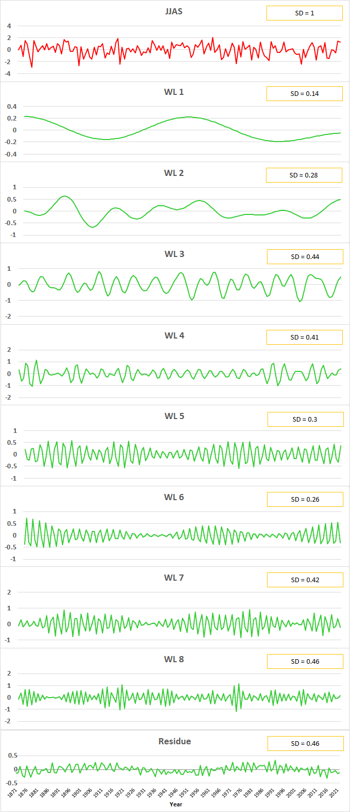
Figure 1: The component time series (labelled WL) obtained by applying EWT

New Scheme to Eliminate Data Leak

Before we proceed to discuss the new scheme developed in this work, it is necessary to draw attention to an inherent difficulty in the use of decomposed data for predicting/forecasting.

Decomposed Data and Information Leak

As mentioned earlier, only if the test data set is kept carefully aside and unseen by the model, the comparison of predictions with observed values will be an effective test of the performance of the model. The pre-requisite for this scheme to work is that the training and the testing data must remain constant so that patterns detected by DNN are fixed. Further, there should be no percolation of information from the test set to the training set. The data leakage problem during one-time decomposition has already been mentioned. Our investigations with JJAS decomposed using the whole data set also confirmed these findings. An analysis of this problem is presented next and is followed by a proposed solution.

Use of Information from Future

The following observation indicates that leak or sharing of information from testing to training set can occur. When a data set is decomposed into component series, the resultant components can change appreciably even when one new data point is added, e.g., when the period of JJAS is changed from 1871-2000 to 1871-2001. This is described below. Let $\mathbb{J}$ be the variable to be predicted from the JJAS data series:

$$\mathbb{J}=\{J_{y_{1}},J_{y_{2}},J_{y_{3}},...,J_{y_{N}}\}$$

where $J_{y_{i}}$ is the rainfall data for the year $y_{i}$. In the present case, $y_{1}$ = 1871 and $y_{N}$ = 2022 for the entire data set. We can model the entire set or subsets of it. We will consider a general case where only a part of the series may be used in calculations. Let the series $\mathbb{J}$ from $y_{n}$ to $y_{m}$ be decomposed into $k$ component series where $y_{n}$ and $y_{m}$ are the first and end years. The data for each component is a value corresponding to a year. Thus, data for the year $y_{l}$ will be the values denoted by $\mathbb{C}_{y_{n},y_{m}}(y_{l},1),\mathbb{C}_{y_{n},y_{m}}(y_{l},2),\ldots\mathbb{C}_{y_{n},y_{m}}(y_{l},k)$. Subscripts indicate a range of data while arguments indicate the year and number of the constituent series. The entire decomposed data of the component series is then a matrix having dimension $(y_{m}-y_{n})\times k$. Let $\mathbb{C}_{y_{n},y_{m}}$ denote the matrix, and the elements are given by $\mathbb{C}_{y_{n},y_{m}}(y_{j},l)$, where  $j=n\,\text{to}\,m$, and  $l=1\,\text{to}\,k$.

$$\mathbb{C}_{y_{n},y_{m}}=\begin{Bmatrix}$$\mathbb{C}_{y_{n},y_{m}}(y_{n},1)&\mathbb{C}_{y_{n},y_{m}}(y_{n},2)&...&\mathbb{C}_{y_{n},y_{m}}(y_{n},k)$$\\ $$\mathbb{C}_{y_{n},y_{m}}(y_{n+1},1)&\mathbb{C}_{y_{n},y_{m}}(y_{n+1},2)&...&\mathbb{C}_{y_{n},y_{m}}(y_{n+1},k)$$\\ \vdots\\ $$\mathbb{C}_{y_{n},y_{m}}(y_{m-1},1)&\mathbb{C}_{y_{n},y_{m}}(y_{m-1},2)&...&\mathbb{C}_{y_{n},y_{m}}(y_{m-1},k)$$\\ $$\mathbb{C}_{y_{n},y_{m}}(y_{m},1)&\mathbb{C}_{y_{n},y_{m}}(y_{m},2)&...&\mathbb{C}_{y_{n},y_{m}}(y_{m},k)$$\end{Bmatrix}$$

Each column of $\mathbb{C}_{y_{n},y_{m}}$ forms a data series, and is like a conventional time series.

When the period of the decomposition changes, even when the starting year $y_{n}$ is fixed, all the individual elements of the data series, i.e., of each of the columns, can change. Thus, if the decomposition is done from year $y_{n}$ to $y_{m+1}$, an additional row comprising of $\mathbb{C}_{y_{n},y_{m+1}}(y_{m+1},l)$ is added to the matrix. The matrix will now be:

$$\mathbb{C}_{y_{n},y_{m+1}}=\begin{Bmatrix}$$\mathbb{C}_{y_{n},y_{m+1}}(y_{n},1)&\mathbb{C}_{y_{n},y_{m+1}}(y_{n},2)&...&\mathbb{C}_{y_{n},y_{m+1}}(y_{n},k)$$\\ $$\mathbb{C}_{y_{n},y_{m+1}}(y_{n+1},1)&\mathbb{C}_{y_{n},y_{m+1}}(y_{n+1},2)&...&\mathbb{C}_{y_{n},y_{m+1}}(y_{n+1},k)$$\\ \vdots\\ $$\mathbb{C}_{y_{n},y_{m+1}}(y_{m-1},1)&\mathbb{C}_{y_{n},y_{m+1}}(y_{m-1},2)&...&\mathbb{C}_{y_{n},y_{m+1}}(y_{m-1},k)$$\\ $$\mathbb{C}_{y_{n},y_{m+1}}(y_{m},1)&\mathbb{C}_{y_{n},y_{m+1}}(y_{m},2)&...&\mathbb{C}_{y_{n},y_{m+1}}(y_{m},k)$$\\ $$\mathbb{C}_{y_{n},y_{m+1}}(y_{m+1},1)&\mathbb{C}_{y_{n},y_{m+1}}(y_{m+1},2)&...&\mathbb{C}_{y_{n},y_{m+1}}(y_{m+1},k)$$\end{Bmatrix}$$

where the elements of this matrix for the first $m$ rows can have values different from those in the matrix obtained from decomposition of the previous year’s data: $\mathbb{C}_{y_{n},y_{m}}(y_{j},l)\neq\mathbb{C}_{y_{n},y_{m+1}}(y_{j},l)$. This was found to be the case with JJAS, and also by others.^{17, 27} This behaviour is illustrated in Figure 2 for one component labelled WL8. Three decompositions from JJAS data were made: 1871-1901, 1871-1902 and 1871-1903 (data shown from 1898). It shows clearly how the component labelled WL8 changes as data of one extra year are added.

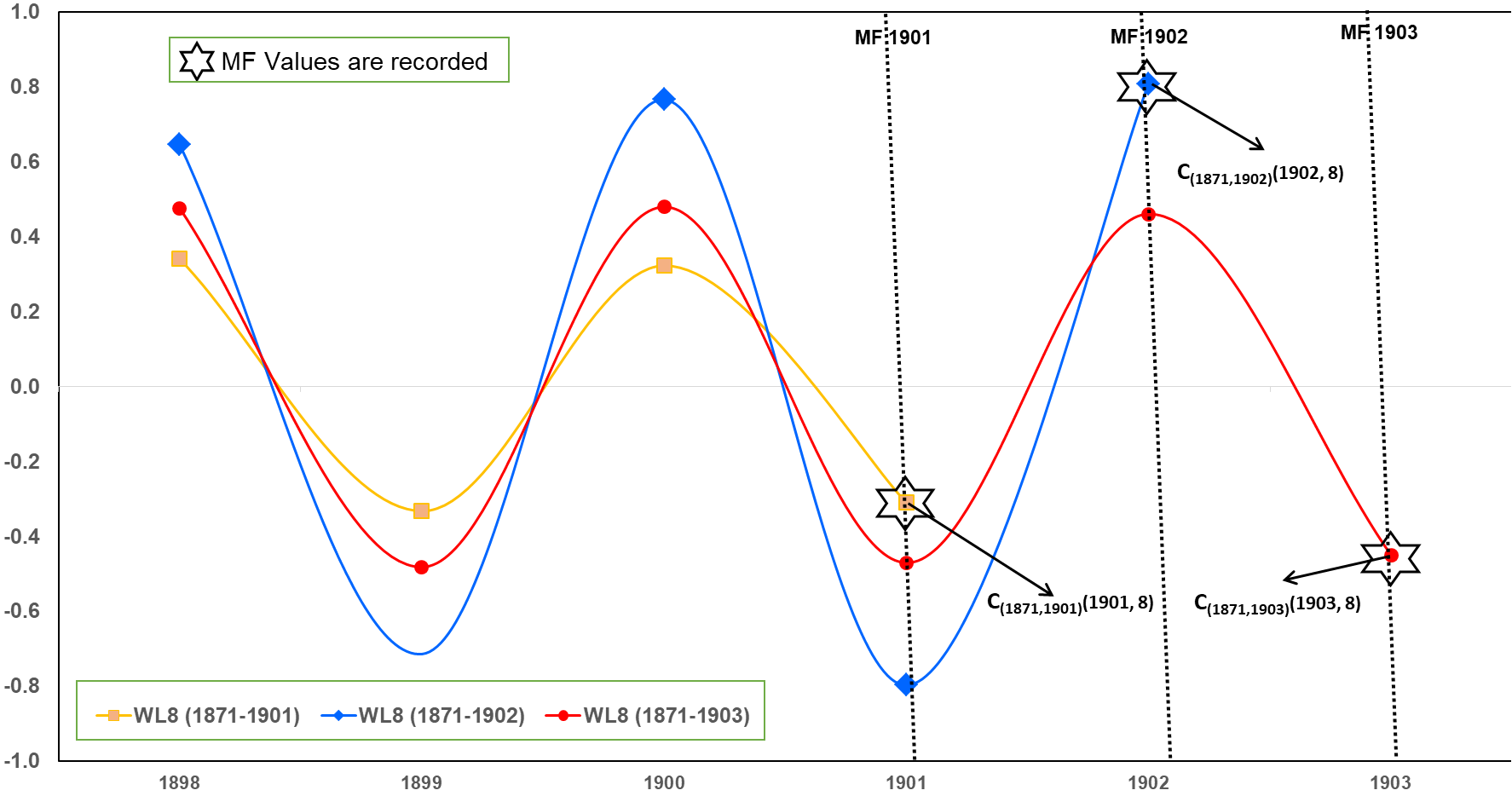
Figure 2: Variation of component labelled WL8 with Progressive Decomposition, Starting with 1901 and ending at 1903

The implication of this is that information on the entire range of data is embedded in all the elements of the matrix obtained by the decomposition of data corresponding to all the years. Thus, even if data for one additional year is added, the information of that year is incorporated into all the coefficients corresponding to earlier years, and the character of all the component series changes. To be precise, the data $\mathbb{C}_{y_{1},y_{m}}$ represent the state of the component series as would finally, be evolved to in the year $y_{m}$. This has two consequences. Firstly, suppose the data from $y_{1}$ to $y_{m}$ of the time-series (e.g., 1871-1901) were divided into training set from $y_{1}$ to $y_{n}$ (e.g., 1871-1891) and the rest $y_{n+1}$ to $y_{m}$ (e.g., 1892-1901) as a testing set, and a model was developed. It could do very well to predict the test data, but that could as well be since information of $y_{n+1}$ to $y_{m}$ (e.g., 1892-1901) was present in all the coefficients from $y_{1}$ up to $y_{n}$ as explained just now. Thus, in one-time decomposition method, both training and testing data are using information from ’future’. Johny et al. ¹⁹, Gao et al. ¹⁷, Huang and Deng ²⁷ had recognized this. It was termed ¹⁷ as data-leakage problem. Secondly, the component series from $y_{1}$ to $y_{n}$ used for training but obtained from years $y_{1}$ to $y_{m}$ are very different from those for the same period ($y_{1}$ to $y_{n}$) but obtained from $y_{1}$ to $y_{m+1}$ of the time series data. Thus, the prediction of JJAS for the year $y_{m+1}$ based on training on the earlier data set cannot be expected to succeed. Thus, a forecast of data of JJAS even for one year beyond the last data point, i.e., for $y_{N+1}$, cannot be expected to be successful based on training and testing of JJAS data from $y_{1}$ to $y_{N}$. While the procedure may succeed in some instances, it cannot be a reliable method.

Proposed Strategy

Changes in the components of the component series (i.e., elements of columns of the matrix $\mathbb{C}_{y_{n},y_{m}}$) when a time series is decomposed after a new data point is added to it are indicative of the difficulties pointed out. These would be resolved if components of a series obtained by decomposition can be made to remain unchanged during progressive decomposition, and only a new element is added to the existing data series with every decomposition. If that can be achieved, a time series can be decomposed, and divided into training and testing sets while ensuring that information from the testing period is not permeating into training period. Then, the time-series can be modelled using the usual method of training and testing, accompanied with the advantages of decomposition into simpler parallel data series that are more amenable to the learning process of the ML algorithms. A successful model can then be used for forecasting with some hope.

We propose the following method to achieve the constancy desired. Some finite period is required to begin the decomposition of rainfall data into component series. Let that be $y_{b}$. Let JJAS data from years $y_{1}$ to $y_{b}$ be decomposed into $k$ component series. The rainfall for year $y_{b}$ is given by

$$J_{y_{b}}=\sum_{l=1}^{k}\mathbb{C}_{y_{1},y_{b}}(y_{b},l)$$

It is to be noted that $J_{y_{b}}$ is part of historical data and is constant, and hence $\mathbb{C}_{y_{1},y_{b}}(y_{b},l)$ are also constant. Now let data for one more year be added, and JJAS data from years $y_{1}$ to $y_{b+1}$ be decomposed into $k$ wavelets. Before the rainfall for year $y_{b+1}$ is given by

$$J_{y_{b+1}}=\sum_{l=1}^{k}\mathbb{C}_{y_{1},y_{b+1}}(y_{b+1},l)$$

and the rainfall for $y_{b}$ is also given by

$$J_{y_{b}}=\sum_{l=1}^{k}\mathbb{C}_{y_{1},y_{b+1}}(y_{b},l)$$

As discussed earlier, $\mathbb{C}_{y_{1},y_{b+1}}(y_{b},l)\neq\mathbb{C}_{y_{1},y_{b}}(y_{b},l)$. The key point of the proposed method is to recognize that we do not have to use $\mathbb{C}_{y_{1},y_{b+1}}(y_{b},l)$ to predict rainfall $J_{y_{b}}$, but instead should use $\mathbb{C}_{y_{1},y_{b}}(y_{b},l)$. The main advantage is that, as pointed out earlier, $\mathbb{C}_{y_{1},y_{b}}(y_{b},l)$ are not affected by the addition of data for $y_{b+1}$, and remain unchanged. Thus, we need to record only $\mathbb{C}_{y_{1},y_{b}}(y_{b},l)$ for the year $y_{b}$ and $\mathbb{C}_{y_{1},y_{b+1}}(y_{b+1},l)$ for the year $y_{b+1}$. The argument can be extended for the years to follow. Thus, we propose that coefficients of component functions for a year corresponding to the rainfall for that year only will be recorded. Those form a time series which can be learned by ML methods. It can be imagined that each component of the series has a front, with the ending discrete value of the component of the series lying on this front. The front moves as more and more data of JJAS are added and decomposed. Let us denote the moving front by MF. Using JJAS data, decomposed using EWT, the MFs are shown in Figure 2 by vertical dotted lines. MF moves year by year, and the ending values at each MF are recorded (denoted by an asterisk in Figure 2). Between successive MFs, the data changes, but for any MF in a particular year, the stored end-point remains constant. Let $\mathbb{E}_{y_{b},y_{N}}$ be the matrix of endpoints so recorded by decomposing JJAS data but beginning from the year $y_{b}$. It will be given by

$$\mathbb{E}_{y_{b},y_{N}}=\begin{Bmatrix}$$\mathbb{C}_{y_{1},y_{b}}(y_{b},1)&\mathbb{C}_{y_{1},y_{b}}(y_{b},2)&...&\mathbb{C}_{y_{1},y_{b}}(y_{b},k)$$\\ $$\mathbb{C}_{y_{1},y_{b+1}}(y_{b+1},1)&\mathbb{C}_{y_{1},y_{b+1}}(y_{b+1},2)&...&\mathbb{C}_{y_{1},y_{b+1}}(y_{2},k)$$\\ \vdots\\ $$\mathbb{C}_{y_{1},y_{N-1}}(y_{N-1},1)&\mathbb{C}_{y_{1},y_{N-1}}(y_{N-1},2)&...&\mathbb{C}_{y_{1},y_{N-1}}(y_{N-1},k)$$\\ $$\mathbb{C}_{y_{1},y_{N}}(y_{N},1)&\mathbb{C}_{y_{1},y_{N}}(y_{N},2)&...&\mathbb{C}_{y_{1},y_{N-1}}(y_{N},k)$$\\ \end{Bmatrix}$$

Note that rainfall for the year $y_{i}$ is given by

$$J_{y_{i}}=\sum_{l=1}^{k}\mathbb{C}_{y_{1},y_{i}}(y_{i},l)$$

Elements of the above matrix are constant during the entire period of JJAS data, as they represent only the endpoints generated by the latest decompositions. Further, if a data point for the next year $y_{N+1}$ is added to JJAS, and it is decomposed into components, a new row with elements $\mathbb{C}_{y_{1},y_{N+1}}(y_{N+1},l)$ will be added but all the other elements of the above matrix will not change. Each column of the matrix is like any conventional time series over the period chosen. Such time series is pictorially represented in Figure 3, where the ending points of the MFs for WL8 are captured for three years.

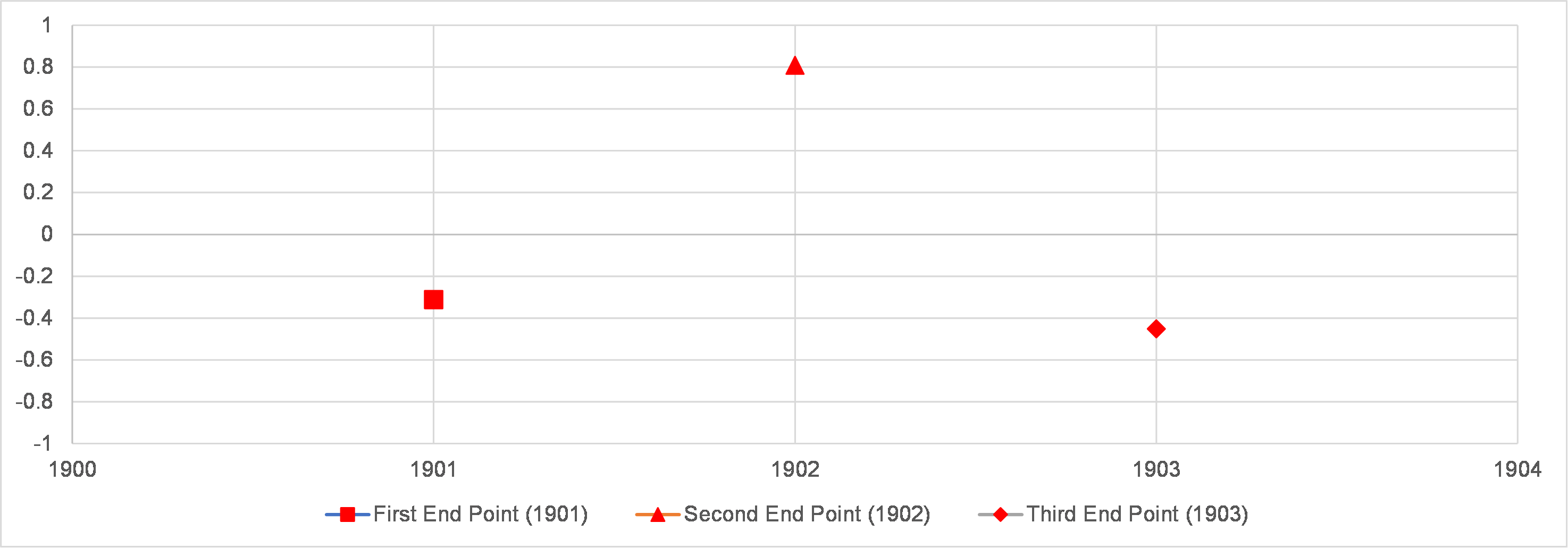
Figure 3: Variation of a component series denoted by WL8

with Progressive Decomposition, Starting with 1901 and ending at 1903

This formulation does not suffer from any of the flaws mentioned before, and the data set can be used to train, test and forecast in the the usual way, without having to worry about leakage of future data. So, this new method applies to other decomposition methods as well, e.g., CEEMDAN, when applied to time series. It is worth describing an alternative view of the moving front method of data collection. It is generally understood that the testing of a model can be considered objective if data in the training set used to develop the model are unbiased by the data in the testing set. As shown above, the coefficients $\mathbb{C}_{y_{1},y_{i}}(y_{i},l),b\leq i\leq n$ in the training data set are unaffected by the coefficients $\mathbb{C}_{y_{1},y_{k}}(y_{k},l),n+1\leq k\leq N$ in the testing set. Thus, one can expect moving front mode of data collection from progressive decomposition to make testing effective.

Nature of Information in the Endpoint Matrix

It is to be noted that when JJAS data during the period $y_{1}$ to $y_{N}$ is decomposed into component series, the matrix $\mathbb{C}_{y_{1},y_{N}}$ will have $(y_{N}-y_{1})\times k$ elements. $\mathbb{E}_{y_{b},y_{N}}$, the matrix generated by storing endpoints, has less number of elements, though the difference can be minimized by choosing the least possible value for $y_{b}$. More importantly, however, the nature of the information contained in the two matrices is different and richer in the latter. The element $\mathbb{C}_{y_{1},y_{N}}(y_{m},l)$ of the former matrix represents the value of the $l^{th}$ component of the series corresponding to the year $y_{m}$ in its evolved state in the year $y_{N}$. The corresponding element in the $\mathbb{E}_{y_{b},y_{N}}$ matrix is $\mathbb{C}_{y_{1},y_{m}}(y_{m},l)$. It on the other hand represents the value of the $l^{th}$ component of the series corresponding to the year $y_{m}$ as it was in its state evolved in the year $y_{m}$. Thus, $\mathbb{E}_{y_{b},y_{N}}$ is recording information of values in states evolved up to some year that lies in the period $y_{b}$ to $y_{N}$. The information contained in $\mathbb{E}_{y_{b},y_{N}}$ is richer but the hope is that a DNN will be capable of learning the hidden patterns. The gain compensating for the additional complexity is the constancy of the elements to the addition of data points, which makes it very amenable to forecasting/predicting. It may also be noted that successive decompositions beginning from year $y_{b}$ are needed to generate the endpoint matrix and hence involves more effort. However, this extra effort is far less compared to that expended in developing entirely new models as practised in walk-forward validation methods, to be discussed later.

The Choice of Deep Learning Network

A Deep Learning Neural Network (DNN) has more than one hidden layer, enabling them to process much more information, and hence it was chosen in this work.

Rainfall is a time series data, and the type of neural network selected has to recognize the time dependency. Recurrent Neural Network (RNN) attempts to do this by taking into consideration the output of the previous time steps also, in addition to the customary input for the current time step. Though in theory, such pristine RNNs can learn arbitrarily long dependencies present in the input sequence, in practice, retaining long-term memory poses a problem with the same. Long Short-Term Memory networks have been developed as an alternative and are used in the present work. A brief description of LSTM is presented in Supplementary information B.

Training, Testing and Forecasting

Consider the JJAS data from year $y_{1}$ to year $y_{N}$. As mentioned earlier, some time is needed to begin decomposition into component series. Let the decomposition start from the year $y_{b}$. Thus, matrix $\mathbb{E}_{y_{b},y_{N}}$ can be formed as described before. Let the data series formed by the elements of columns of that matrix be divided into training set from $y_{b}$ to $y_{TR}$ and a testing set from $y_{TR+1}$ to $y_{TE}$. The rest of the data, i.e. $y_{TE+1}$ to $y_{N}$, are set aside for one-time forecasting and forecasting using Walk Foreward Validation (WFV) It is once again emphasized that elements of the submatrix $\mathbb{E}_{y_{b},y_{TR}}$ are not influenced in any way by the elements of the submatrix $\mathbb{E}_{y_{TR+1},y_{TE}}$. Therefore, the conventional method of splitting the data into training and testing, sets provide a valid test of the model. Each of the $k$ data series will show patterns of variation. If these patterns could be learnt by an ML model, they can be used to make predictions of rainfall for each year in the testing period As $\mathbb{E}_{y_{TE+1},y_{N}}$ are kept separate from both testing and training, and are independent of the other elements, they can be used for evaluating the effectiveness of a developed model in forecasting as well.

The Calculation Scheme of LSTM

The standard multivariate LSTM is implemented, which is diagrammatically in Supplementary Material D.

Computational Specifics of Predictions by EWT-MF-LSTM

Each column of the matrix $\mathbb{E}_{y_{b},y_{N}}$ are the sub-series that are used as independent variables. The matrix $\mathbb{P}_{y_{b},y_{N}}=$ is obtained by combining with the $\mathbb{J}$ vector (dependent variable):

$$\mathbb{P}_{y_{b},y_{N}}=\begin{Bmatrix}$$\mathbb{C}_{y_{1},y_{b}}(y_{b},1)&\mathbb{C}_{y_{1},y_{b}}(y_{b},2)&...&\mathbb{C}_{y_{1},y_{b}}(y_{b},k),\ J_{y_{1}}$$\\ $$\mathbb{C}_{y_{1},y_{b+1}}(y_{b+1},1)&\mathbb{C}_{y_{1},y_{b+1}}(y_{b+1},2)&...&\mathbb{C}_{y_{1},y_{b+1}}(y_{2},k,\ J_{y_{2}}$$\\ \vdots\\ $$\mathbb{C}_{y_{1},y_{N-1}}(y_{N-1},1)&\mathbb{C}_{y_{1},y_{{N-1}}}(y_{N-1},2)&...&\mathbb{C}_{y_{1},y_{N-1}}(y_{N-1},k),\ J_{y_{(N-1)}}$$\\ $$\mathbb{C}_{y_{1},y_{N}}(y_{N},1)&\mathbb{C}_{y_{1},y_{N}}(y_{N},2)&...&\mathbb{C}_{y_{1},y_{N-1}}(y_{N},k),\ J_{y_{N}}$$\\ \end{Bmatrix}$$

These parallel time series, i.e. the columns in the matrix $\mathbb{P}_{y_{b},y_{N}}$ were re-framed as a supervised learning problem by transforming the sequence in the form of input and output pairs using lag value. As mentioned earlier, some finite period is needed to create a component of the series, and end-point collection can start. Thus, 1901 was chosen as the starting point. Out of available data (1871-2022), eight component series and one residue were extracted by progressive decomposition using EWT-MF, ultimately forming nine ($k$ = 9) parallel series of end data points, the points for the period 1901-1980 were devoted to training and the next 1981 to 1999 as testing. The data from 2000 to 2022 were reserved for forecasting.

As mentioned before, a lag period ($\mathit{L}$) or window size was used in re-framing the data $\mathbb{P}$ into a supervised learning problem. Different window sizes, number of hidden layers, number of nodes in each layer, learning rate, tolerable number of epochs to allow a monotonic increase of error before the training is stopped, batch size and so on are varied interactively using experience. The mentioned parameters are called hyperparameters and their values are not known a-priori and must be found by trial and error. Grid search for the above parameters was not conducted, as it is computationally very expensive. The model is trained by using EWT-MF-LSTM data during the period 1901-1980.

For each row of the supervised data of independent variable (in a pre-defined tensor format) input to LSTM, it makes predictions for rainfall for each row. When the last $\mathit{L}$ rows of supervised data of independent variable (again in a particular tensor format), are input to LSTM, it makes one unknown future forecast for rainfall.

The testing period was defined as 1981-1999. The trained model was evaluated against the test set. If the error between actual and predicted values is tolerable, the model is frozen. Otherwise, the model is re-built with modified hyperparameters and the valuation is done against the testing set.

Next, the satisfactory model obtained from the above step is trained for the entire data from 1901-1999, keeping the model hyperparameters to be the same, to arrive at the model that is ready for forecasting from 2000-2022. It is customarily referred to as the final model.

Stochastic Nature

ANN solutions are non-deterministic because they use random numbers for (a) the initialization of weights attached to each node of the network (b) the optimization of weights to solve by Gradient Descent method. This implies that a different pathway will be followed when the same algorithm with the same data is repeatedly run, resulting in a slightly different solution. The randomness can be stopped by specifying a random seed. However, the recommended practice in Data Science is to run the same program with the same data an appreciable number of times and then calculate the result as the average of all the runs. The number of repeated runs has been chosen as 20 since beyond that there is no appreciable difference.

Programming Language and Packages Used

As mentioned earlier LSTM was the choice of deep learning to deal with the high variability of rainfall data. To this end, a description of the programming language and the packages used are described here. Python 3.9 was used to develop the computer program utilizing the available packages: numpy, pandas, numpy, sklearn, pickle, statsmodels, matplotlib, seaborn, statistics.

Python package of EWT (ewtpy) is available at https://pypi.org/project/ewtpy/. Keras, an open-source deep-learning Application Programming Interface (API) (https://pypi.org/project/keras/) written in Python was used to train and predict LSTM networks. Keras acts as an interface for the TensorFlow (https://www.tensorflow.org/install/pip) library, developed by Google Brain. The versions of Keras and Tensorflow were 2.4.3 and 2.4.0 respectively.

Results & Discussion

The section is divided into three parts. We begin by presenting results obtained from the application of the LSTM model developed in the present work. It is followed by a discussion of other models reported in the literature. Finally, predictions by statistical methods are presented.

Predictions of EWT-MF-LSTM model

The Moving Front (MF) data started in 1901. Table 2 shows the duration of the training, testing and forecasting (WFV without and with retraining).

The year ranges are shown in Table 2.

Table 2: Training, Testing and Forecasting Periods

[rgb] .753, 0, 0 Training	Testining	Forecasting
1901-1980	1981-1999	2000-2022

The corresponding $PP$ values are listed in Table Predictions of EWT-MF-LSTM model.

Table 3: $PP$ Values

[rgb] 0, 0, .4                                Training				Testining	Forecasting
[rgb] 0, 0, .4		WFV (No Retraining)	WFV (Retraining)
0.99	0.86	0.90	0.95

The observed versus predicted values are plotted in Figure 4, 5 and 6, for training, testing and the final models.

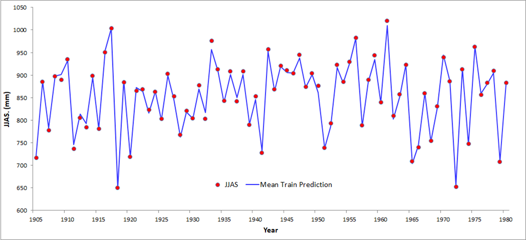
Figure 4: Observations and model predictions during training period

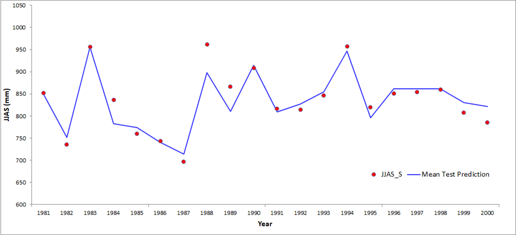
Figure 5: Observations and model predictions during the period assigned for testing.

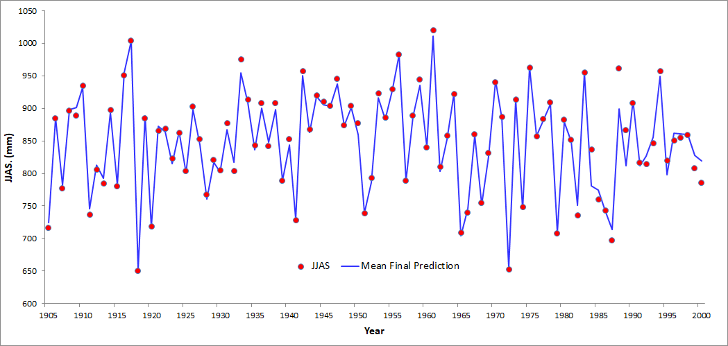
Figure 6: Observations and predictions of the final model for the training and testing period.

The red points are the observed values, and the Blue lines represent predictions. The reported value is obtained by repeating the same experiment 20 times as discussed before.

Forecasting and Comparison with the Other Models

As discussed earlier, when multiple rows of the supervised data, in a compatible tensor format is input to the trained (or final) model, the same number of predictions/forecasts for $JJAS$ are obtained. Thus, if the data from 2000-2022 are fed to the final model (which has been trained using data from 1901-1999), 23 years of forecasts are obtained, at a time. In Figure 7, the Green line represents these forecasts. The $PP$ of these forecasts were 0.90. It is to be noted that this is an in-sample forecast and serves the purpose of determining the efficacy of the learning by DNN, without the influence of training and testing data set. Since $JJAS$ is already known for the period 2000-2022, and hence the EWT-MF points, it cannot be called a true forecast.

Another way suggested uses methods that are referred to in general as Walk Forward Validation (WFV) techniques. In the most widely practised method, the model is trained with all the data up to the latest available to make a forecast for the next year. When an observation for this forecast becomes available next year, the model is updated to include that value, and a forecast is made for the following year. Hence the name WFV. This process yields a forecast, one year at a time. This method is followed in this work for the same forecasting period (2000-2022). The WFV forecasts are presented in Figure 7 in colour Blue. The attained $PP$ = 0.95 is higher than when WFV was not used and can be considered very good.

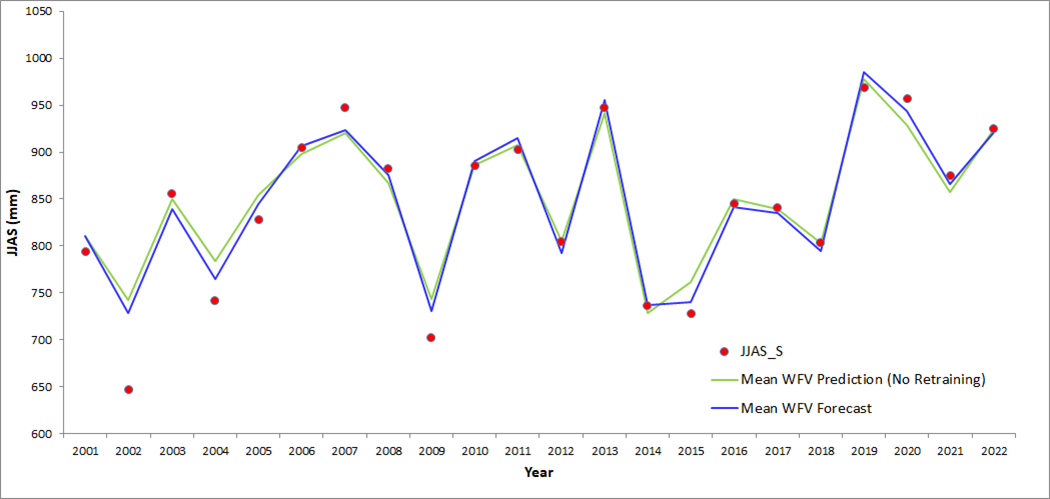
Figure 7: WFV Forecasts without and with retraining

When WFV, with retraining at each step, is applied using EWT-MF forecast data from 2000-2022, the LSTM has a better chance to learn the variations of the EWT-MF components, since it is progressively retrained with the addition of the forecast data one at a time. This variation can be learnt during the training phase, but not necessarily completely, as the model becomes more and more skilful with the added data. For retraining progressively by adding forecast data one by one, all other hyperparameters are kept the same, i.e. no new model was generated. It is pertinent to add that, instead of feeding all 23 years of supervised data at once, one set of supervised rows can be input at a time, just like WFV, but no retraining is done. This also results in the same output values as before (23 years at a time) with a $PP$ of 0.90.

Earlier work on different forecasting strategies that used decomposition techniques is discussed here. It is difficult to compare the present work with others since decomposition strategies and neural network models are different. The comparison is presented to simply give an idea of the relative performances.

Some simpler routes have been tried to avoid the leakage of future information. In one such, all the available data are decomposed once only, and the constituent series are trained and used to make predictions, e.g., JJAS data from 1901-2022 followed by a forecast for 2023. However, the reliability of such a model is unknown in the absence of any evaluation procedure. Further, a model developed by minimising only the training error often results in an over-fitted model.

Iyengar and Kanth ²⁸ divided JJAS data into training and forecast sets. Forecasts were made by a combination of regression and the walk-forward method. Details of training have not been provided, but they report a $PP$ of 0.83 for training. This may be compared with a $PP$ of 0.90 reached during testing in this work. It is also worth noting that they attained a $PP$ of 0.82 for the forecast set, which is nearly the same as that for training. This is a much poorer performance compared to that obtained for forecast in the present work.

Johny et al. ¹⁹ developed another variation of WFV. After dividing the data into training and testing, the training data is divided into a quasi-training and quasi-testing set. A model is developed ignoring the fact that both the quasi-train and quasi-test set will contain future information. They then proceed to use the saved trained model to make a forecast for one year. Redecomposition is made after including the actual value of the forecasted year, followed by retraining and another forecasting. As the saved model is used, i.e. no change in the model is done, though test data with data leak are being used, it is the closest to compare with the present work. They do not report $PP$ for the forecast period. However, the Mean Absolute Error reported can be used in place of RMSE to estimate $PP$. It is about 0.8, lower than what was obtained in this work. Johny et al. ¹⁹ also used another strategy, referred to as AEEMD, where an entirely new model is developed every time a data point is added from the test set, to make forecasts. A $PP$ of these forecasts is estimated from their parity plots to be 0.75, a value near that of $PP$ for forecasts.

Predictive/forecasting capability of the present EWT-MF-LSTM method is compared with that of others in Table 4. Here the performance numbers quoted are as reported by the respective authors and, if it was not reported by the authors it was computed from the values provided by them where possible. As can be seen, the present method does achieve better accuracy than other methods.

Table 4: Broad comparison of the performance of predictive capabilities of models

Reference	Rainfall Data	Training	Testing	Method	Future Prediction	RMSE (mm)	NRMSE	MAPE	R	$PP$
Hybrid models: present and others
Present Work	1871-2022	1901-1999	2000-2022	EWT-MF-LSTM		4.49	0.005	0.0039	0.997	0.95
Johny et al. 19	1871-2018	1871-1970	1971-2018	AEEMD-ANN			0.14		0.91	0.75
Iyengar and Kanth 28	1871-1994	1872-1990	1991-2003	EMD-NN-Regression	1 year					0.82
* Acronyms:
EWT: Empirical Wavelet Transform
MF: Moving Front
LSTM: Long Short-Term Memory
AEEMD: Adaptive Ensemble Empirical Mode Decomposition
ANN: Artificial Neural Network
EMD: Empirical Mode Decomposition

Conclusions

Complex time series have very high variability, and due to their highly non-linear complex nature, not even DNN alone may be insufficient to learn and forecast it with high accuracy. In such instances, many researchers in different domains employed the decomposition of the parent time series into simpler constituent series using signal processing tools like EMD, EEMD, CEEMDAN, EWT and VMD. The idea is to learn the sub-series individually and then sum up the individual predictions to reproduce the original time series or to formulate a multivariate problem. Decomposition of the whole dataset only once and dividing it into training and testing sets is widely practised in literature. However, a property of the one-time decomposition technique is that each of the sub-series changes its nature depending upon the starting and ending period. This leads to leakage of future information, making the whole testing process ineffective, and has been referred to as a ’data leak’. A novel MF method has been proposed in this work to prevent the data leak so that the decomposed constituent time series can be treated as normal time series and reap the benefits of decomposition as well. The technique employs progressive decomposition and collection of endpoints at each step. ISMR data was selected to demonstrate the efficacy of the MF method. EWT was found to be superior to CEEMDAN and was used to decompose ISMR data employing the MF method. Instead of using the conventional univariate technique of learning decomposed time series individually, a multivariate formulation is employed in the present work. Here, the constituent series form a parallel independent series with the target time series as the dependent one. State-of-the-art LSTM network architecture with superior sequence predictive capabilities was used in this work. The entire data was divided into training, testing and forecasting periods. The performance of the resulting MF-EWT-LSTM model was excellent in training and testing. Forecasts were obtained by a finalized model all at once and also using a walk-forward method widely used in the literature. The results obtained were much superior to those reported in the literature.

Supplementary Material

A. Statistical Properties

The probability density function revealed a skewed distribution. Almost no (or very weak) autocorrelation was found, and this explains why the linear time-series modelling failed. "Stationarity" has to be ascertained, and any trend and/or seasonal effects are to be removed before beginning neural network modelling of time-series data. The seasonal_decompose the function of the Python package statsmodels has been used to determine "seasonality" (a data science term), it was found seasonal component was absent. This was to be expected as the data was the seasonal average.

The Augmented Dickey-Fuller (ADF) test by Said and Dickey ²⁶ is a common statistical test to determine how strongly a time series is defined by a trend. The result of this test is interpreted using the $p$-value. Using a Python function adfuller from the statsmodels package, the $p$-value was found to be zero for the JJAS, and it is inferred that the time series is stationary. Hence, the data, as retrieved, were used as the input to the forecasting models.

B. Long Short-Term Memory (LSTM)

RNNs using Long Short-Term Memory (LSTM) units can decide whether to keep the long-term memory or not. LSTMs use a series of gates (Forget Gate, Input Gate and Output Gate) and a new-memory block which controls how the sequential information enters and leaves the network while retaining the relevant memory. This enables LSTM to allow the previously mentioned gradients to flow unchanged, thereby partially solving the vanishing gradient problem. LSTM was proposed by Hochreiter and Schmidhuber ²⁹. Google, Apple, Amazon, Facebook and Microsoft are among the giant companies that use LSTM, and it, therefore, is a time-tested neural network with a significant ability to predict sequential data. It is chosen in this work also. The gates in the LSTM mentioned and the New Memory block is all neural networks in themselves and all of them receive the same two inputs: the previous hidden state $h_{t-1}$, and input for the current step $x_{t}$. The outputs of the Forget, Input and Output are $f$, $i$ and $o$, suffixed by the time step $t$. At the very end, the hidden state $h_{t}$ is converted to the final result by a linear layer to give the actual predicted value $\hat{y}_{t}$:

^y_t = W h_t

The equations below, for the forward pass, are presented below. The influence of bias has not been taken into account.

Equations for the forward pass of LSTM are:

$$f_{t} =\sigma(W_{f}x_{t}+U_{f}h_{t-1})$$

$$i_{t} =\sigma(W_{i}x_{t}+U_{i}h_{t-1})$$

$$o_{t} =\sigma(W_{o}x_{t}+U_{o}h_{t-1})$$

$$\tilde{c}_{t} =\sigma(W_{c}x_{t}+U_{c}h_{t-1})$$

$$c_{t} =f_{t}\circ c_{t-1}+i_{t}\circ\tilde{c}_{t}$$

$$h_{t} =o_{t}\circ\sigma_{h}(c_{t})$$

where the initial values are ${\displaystyle c_{0}=0}$ and ${\displaystyle h_{0}=0}$ and the operator ${\displaystyle\circ}$ denotes the element-wise product. The subscript ${\displaystyle t}$ indexes the time step. Further,

${\displaystyle x_{t}}$ : Input vector to the LSTM unit ${\displaystyle f_{t}}$ : Output vector of the Forget Gate ${\displaystyle i_{t}}$ : Output vector of the Input Gate ${\displaystyle o_{t}}$ : Output vector of the Output Gate ${\displaystyle h_{t}}$ : Hidden state vector is also known as the output vector of the LSTM unit ${\displaystyle{\tilde{c}}_{t}}$ : Output vector of the New memory cell ${\displaystyle c_{t}}$ : Cell state vector ${\displaystyle W}$, ${\displaystyle U}$ : Weight matrices which are adjusted during training

The Activation functions are:

${\displaystyle\sigma}$ : Sigmoid function ${\displaystyle tanh}$ : Hyperbolic tangent function

C. Comparison of Data Decomposition Methods

As discussed before, CEEMDAN is the most effective technique in the EMD family, and this was chosen to decompose JJAS data. However, with the LSTM network and CEEMDAN decomposition described above, the predictive capability was not satisfactory. This prompted an investigation to find out possible reasons for the lack of improvement. The first IMF (IMF1) computed by CEEMDAN appeared to account for most of the non-linearity of JJAS as indicated by the graphs of the IMFs. The comparison is shown in the left panel of Figure 1.

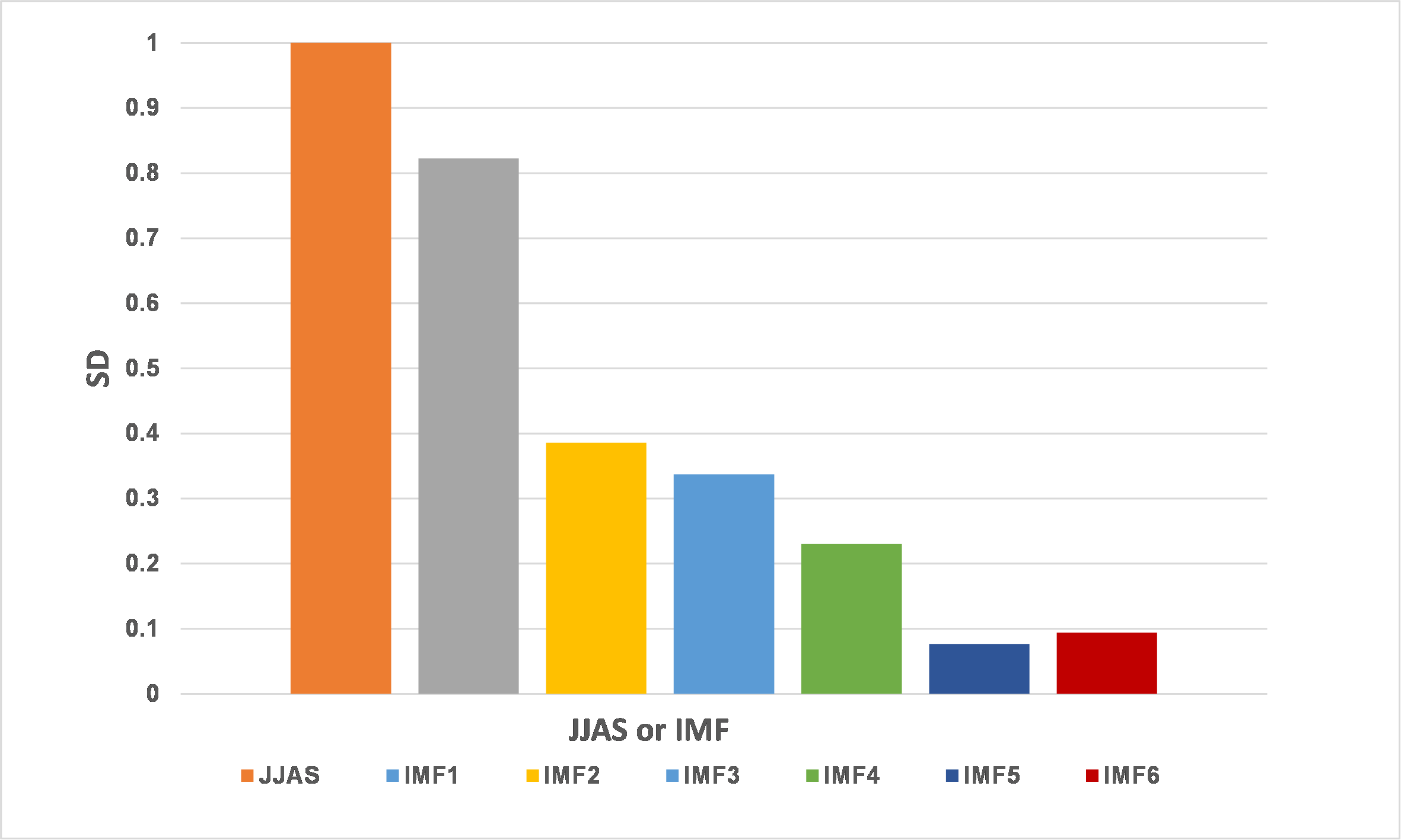
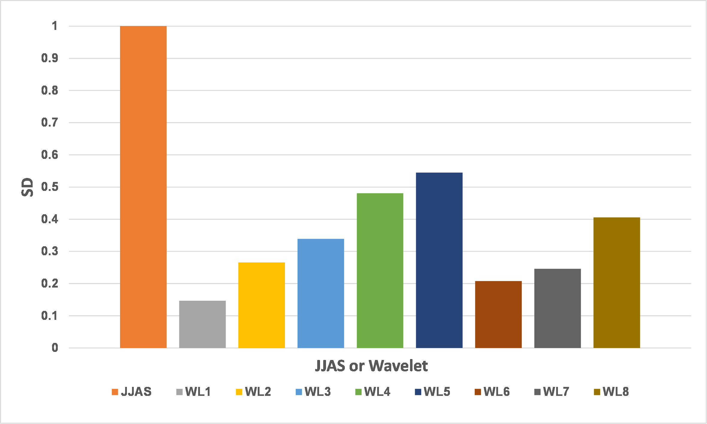
Figure 1: Left panel shows a comparison of Standard Deviations (SD) of JJAS with that of the IMFs extracted using CEEMDAN. Right panel shows a comparison of Standard Deviations (SD) of JJAS with that of Wavelets extracted using EWT.

It is evident from the figure that IMF1 contained the majority of the high amplitude components, making it difficult to learn by ANN. A better distribution is not possible since the EMD/EEMD/CEEMDAN algorithms fixed the number of IMFs automatically determined. Lack of improvement in $\mathit{PP}_{Test}$ can be attributed to the inability of the CEEMDAN algorithm to distribute the variances in the original signal into a large number of less complex components. Secondly, it was observed that the LSTM network could not predict IMF1 with the desired accuracy. This indicated the complexity of the patterns in IMF1 was so high that it was not amenable even to the sophisticated deep learning LSTM networks.

As mentioned earlier, a higher number of modes can be specified with EWT. Hence, EWT was tried as an alternative to decompose JJAS. The right panel of Figure 1 shows the SD for different wavelets obtained versus the SD of the rainfall data, after extracting 8 modes by EWT. It is evident from Figure 1, the fluctuations in JJAS are more evenly distributed among the decomposed time series for EWT as shown in Figure 1.

D. Calculation Scheme

Figure 2 shows the flow diagram. The JJAS data, first scaled using the mean and the SD, was decomposed by the decomposition algorithm (EWT) into the $k$ constituent simpler time series, following the MF method described earlier. Each such time series was input to $k$ dimensional multi-variate LSTM network, for training and making predictions. The prediction is inversely scaled to get the predicted JJAS.

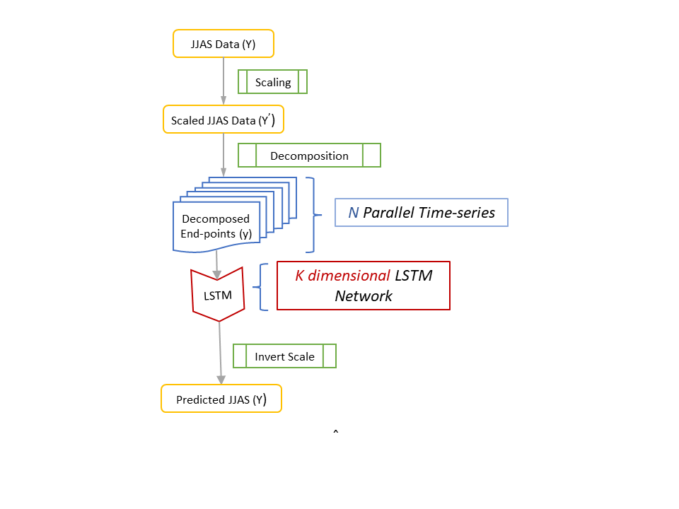
Figure 2: The calculation flow diagram

Statements and Declarations

• Acknowledgements: The author sincerely thanks Profs. J. Srinivasan of Divecha Center for Climate Change, Indian Institute of Science, Bangalore, and K.S. Gandhi, Department of Chemical Engineering, Indian Institute of Science, Bangalore, for insightful discussions and critical comments on the manuscript. Also, I thank Prof. K.V.S. Hari, Department of ECE, Indian Institute of Science, Bangalore, for his expert comments on the method proposed.

• Funding: The author declares that no funds, grants, or other support were received during the preparation of this manuscript.

• Competing interests: The authors have no competing interests to declare that are relevant to the content of this article.

• Compliance with Ethical Standards: The research meets all ethical guidelines, including adherence to the legal requirements of the study country.

• Consent to participate: Not applicable.

• Consent for publication: The author agrees with the content and gave explicit consent to submit and that he obtained consent from the responsible authorities at the Indian Institute of Science, where the work has been carried out before the work is submitted.

• Availability of data and materials: The rainfall data from the year 1871 to 2016 and 2017 to 2022 were obtained from the Indian Institute of Tropical Meteorology (IITM) and Indian Meteorological Department’s (IMD) websites respectively.

• Research involving Human Participants and/or Animals: Not applicable.

References

- Zhang et al. 2008 Xun Zhang, K.K. Lai, and Shou-Yang Wang. A new approach for crude oil price analysis based on empirical mode decomposition. Energy Economics, 30(3):905–918, May 2008. doi: 10.1016/j.eneco.2007.02.012. URL https://doi.org/10.1016/j.eneco.2007.02.012.
- Bai et al. 2009 Weili Bai, Zhigang Liu, Dengdeng Zhou, and Qi Wang. Research of the load forecasting model base on HHT and combination of ANN. In 2009 Asia-Pacific Power and Energy Engineering Conference. IEEE, March 2009. doi: 10.1109/appeec.2009.4918671. URL https://doi.org/10.1109/appeec.2009.4918671.
- Liu et al. 2012 Hui Liu, Chao Chen, Hong qi Tian, and Yan fei Li. A hybrid model for wind speed prediction using empirical mode decomposition and artificial neural networks. Renewable Energy, 48:545–556, December 2012. doi: 10.1016/j.renene.2012.06.012. URL https://doi.org/10.1016/j.renene.2012.06.012.
- Wei and Chen 2012 Yu Wei and Mu-Chen Chen. Forecasting the short-term metro passenger flow with empirical mode decomposition and neural networks. Transportation Research Part C: Emerging Technologies, 21(1):148–162, April 2012. doi: 10.1016/j.trc.2011.06.009. URL https://doi.org/10.1016/j.trc.2011.06.009.
- Ghelardoni et al. 2013 Luca Ghelardoni, Alessandro Ghio, and Davide Anguita. Energy load forecasting using empirical mode decomposition and support vector regression. IEEE Transactions on Smart Grid, 4(1):549–556, March 2013. doi: 10.1109/tsg.2012.2235089. URL https://doi.org/10.1109/tsg.2012.2235089.
- Ren et al. 2015 Ye Ren, P. N. Suganthan, and Narasimalu Srikanth. A comparative study of empirical mode decomposition-based short-term wind speed forecasting methods. IEEE Transactions on Sustainable Energy, 6(1):236–244, January 2015. doi: 10.1109/tste.2014.2365580. URL https://doi.org/10.1109/tste.2014.2365580.
- Wang et al. 2016 Shouxiang Wang, Na Zhang, Lei Wu, and Yamin Wang. Wind speed forecasting based on the hybrid ensemble empirical mode decomposition and GA-BP neural network method. Renewable Energy, 94:629–636, August 2016. doi: 10.1016/j.renene.2016.03.103. URL https://doi.org/10.1016/j.renene.2016.03.103.
- Zhang et al. 2016 Chi Zhang, Haikun Wei, Junsheng Zhao, Tianhong Liu, Tingting Zhu, and Kanjian Zhang. Short-term wind speed forecasting using empirical mode decomposition and feature selection. Renewable Energy, 96:727–737, October 2016. doi: 10.1016/j.renene.2016.05.023. URL https://doi.org/10.1016/j.renene.2016.05.023.
- Huang and Deng 2021a Yusheng Huang and Yong Deng. A new crude oil price forecasting model based on variational mode decomposition. Knowledge-Based Systems, 213:106669, February 2021a. doi: 10.1016/j.knosys.2020.106669. URL https://doi.org/10.1016/j.knosys.2020.106669.
- Bisoi et al. 2019 Ranjeeta Bisoi, P.K. Dash, and S.P. Mishra. Modes decomposition method in fusion with robust random vector functional link network for crude oil price forecasting. Applied Soft Computing, 80:475–493, July 2019. doi: 10.1016/j.asoc.2019.04.026. URL https://doi.org/10.1016/j.asoc.2019.04.026.
- Li et al. 2019 Jinchao Li, Shaowen Zhu, and Qianqian Wu. Monthly crude oil spot price forecasting using variational mode decomposition. Energy Economics, 83:240–253, September 2019. doi: 10.1016/j.eneco.2019.07.009. URL https://doi.org/10.1016/j.eneco.2019.07.009.
- E et al. 2017 Jianwei E, Yanling Bao, and Jimin Ye. Crude oil price analysis and forecasting based on variational mode decomposition and independent component analysis. Physica A: Statistical Mechanics and its Applications, 484:412–427, October 2017. doi: 10.1016/j.physa.2017.04.160. URL https://doi.org/10.1016/j.physa.2017.04.160.
- Zhou et al. 2019 Yingrui Zhou, Taiyong Li, Jiayi Shi, and Zijie Qian. A CEEMDAN and XGBOOST-based approach to forecast crude oil prices. Complexity, 2019:1–15, February 2019. doi: 10.1155/2019/4392785. URL https://doi.org/10.1155/2019/4392785.
- Yang et al. 2019 Hua Yang, Yunfei Zhang, and Feng Jiang. Crude oil prices forecast based on EMD and BP neural network. In 2019 Chinese Control Conference (CCC). IEEE, July 2019. doi: 10.23919/chicc.2019.8866586. URL https://doi.org/10.23919/chicc.2019.8866586.
- Lahmiri 2017 Salim Lahmiri. Comparing variational and empirical mode decomposition in forecasting day-ahead energy prices. IEEE Systems Journal, 11(3):1907–1910, September 2017. doi: 10.1109/jsyst.2015.2487339. URL https://doi.org/10.1109/jsyst.2015.2487339.
- Wang and Wu 2016 Y. Wang and L. Wu. On practical challenges of decomposition-based hybrid forecasting algorithms for wind speed and solar irradiation. Energy, 112:208–220, 2016. doi: 10.1016/j.energy.2016.06.075. URL https://doi.org/10.1016/j.energy.2016.06.075.
- Gao et al. 2021 Ruobin Gao, Liang Du, Kum Fai Yuen, and Ponnuthurai Nagaratnam Suganthan. Walk-forward empirical wavelet random vector functional link for time series forecasting. Applied Soft Computing, 108:107450, sep 2021. doi: 10.1016/j.asoc.2021.107450. URL https://doi.org/10.1016%2Fj.asoc.2021.107450.
- Iyengar and Kanth 2004 R. N. Iyengar and S. T. G. Raghu Kanth. Intrinsic mode functions and a strategy for forecasting indian monsoon rainfall. Meteorology and Atmospheric Physics, 90(1-2):17–36, July 2004. doi: 10.1007/s00703-004-0089-4. URL https://doi.org/10.1007/s00703-004-0089-4.
- Johny et al. 2020 K. Johny, M.L. Pai, and S. Adarsh. Adaptive EEMD-ANN hybrid model for indian summer monsoon rainfall forecasting. Theoretical and Applied Climatology, 141(1-2):1–17, March 2020. doi: 10.1007/s00704-020-03177-5. URL https://doi.org/10.1007/s00704-020-03177-5.
- Sahay and Srivastava 2014 R.R. Sahay and A. Srivastava. Predicting monsoon floods in rivers embedding wavelet transform, genetic algorithm and neural network. Water Resources Management, 28(2):301–317, December 2014. doi: 10.1007/s11269-013-0446-5. URL https://doi.org/10.1007/s11269-013-0446-5.
- Ramana et al. 2013 R.V. Ramana, B. Krishna, S. R. Kumar, and N. G. Pandey. Monthly rainfall prediction using wavelet neural network analysis. Water Resources Management, 27(10):3697–3711, June 2013. doi: 10.1007/s11269-013-0374-4. URL https://doi.org/10.1007/s11269-013-0374-4.
- Azad et al. 2015 S. Azad, S. Debnath, and M. Rajeevan. Analysing predictability in indian monsoon rainfall: A data analytic approach. Environmental Processes, 2(4):717–727, September 2015. doi: 10.1007/s40710-015-0108-0. URL https://doi.org/10.1007/s40710-015-0108-0.
- Huang et al. 1998 N.E. Huang, Z. Shen, S.R. Long, M.C. Wu, H.H. Shih, Q. Zheng, Nai-Chyuan Yen, C.C. Tung, and H.H. Liu. The empirical mode decomposition and the hilbert spectrum for nonlinear and non-stationary time series analysis. Proceedings of the Royal Society of London. Series A: Mathematical, Physical and Engineering Sciences, 454(1971):903–995, March 1998. doi: 10.1098/rspa.1998.0193. URL https://doi.org/10.1098/rspa.1998.0193.
- Beltrán-Castro et al. 2013 J. Beltrán-Castro, J. Valencia-Aguirre, M. Orozco-Alzate, G. Castellanos-Domínguez, and C.M. Travieso-González. Rainfall forecasting based on ensemble empirical mode decomposition and neural networks. In Advances in Computational Intelligence, pages 471–480. Springer Berlin Heidelberg, 2013. doi: 10.1007/978-3-642-38679-4_47. URL https://doi.org/10.1007/978-3-642-38679-4_47.
- Basak 2020 P. Basak. Forecasting of summer monsoon rainfall over gangetic west bengal, india utilising intrinsic mode functions, linear and neural regression. Journal of Modeling and Optimization, 12(1):60–69, June 2020. doi: 10.32732/jmo.2020.12.1.60. URL https://doi.org/10.32732/jmo.2020.12.1.60.
- Said and Dickey 1984 S.E. Said and D.A. Dickey. Testing for unit roots in autoregressive-moving average models of unknown order. Biometrika, 71(3):599–607, 1984. doi: 10.1093/biomet/71.3.599. URL https://doi.org/10.1093/biomet/71.3.599.
- Huang and Deng 2021b Yusheng Huang and Yong Deng. A new crude oil price forecasting model based on variational mode decomposition. Knowledge-Based Systems, 213:106669, feb 2021b. doi: 10.1016/j.knosys.2020.106669. URL https://doi.org/10.1016%2Fj.knosys.2020.106669.
- Iyengar and Kanth 2003 R.N. Iyengar and S. T. Kanth. Empirical modelling and forecasting of indian monsoon rainfall. Current Science, 85(8):1189––1201, 2003. URL www.jstor.org/stable/24108618.
- Hochreiter and Schmidhuber 1997 S. Hochreiter and J. Schmidhuber. Long short-term memory. Neural Computation, 9(8):1735–1780, 1997.