Rate-Distortion Analysis for Semantic-Aware Multi-Terminal Source Coding Problem

Abstract

A novel distributed source coding model which named semantic-aware multi-terminal source coding problem is proposed and studied in the paper. This is motivated by the new communication paradigm being aware of semantic information, in which invisible semantic features are observed by multiple agents, and both semantic and observation reconstructions are imposed distortion constraints. The theoretical analysis of this model is provided in this work, in which we present a generalized Berger-Tung based sum rate region considering the semantic source, and further obtain upper and lower bounds when sources are joint Gaussian distributed. Under this case, the tradeoff between two distortions and optimal rate allocation scheme are discussed. Moreover, since the model couples the conventional multi-terminal coding and CEO problems, the degeneration of generalized bounds to existing works are shown. Finally, we also present the sum rate bounds in special cases when sources are Bernoulli and distortion measure adopts logarithmic loss.

I Introduction

In nowadays sixth-generation (6G) networks, semantic-aware communications emerge with superiorities on high compression ratio and transmission efficiency in comparison with the conventional ones. This is mainly attributed to that the meanings and intents of the source information are considered, hence the correlation among semantics largely reduces the redundancy and promotes the transmission efficiency. In such semantic-aware communications, the key problems are how to describe semantic information and design semantic source coding schemes. Therefore, theoretical models on characterizing semantic information and heuristic coding schemes are urgently required.

The conception of communication over semantic level was first presented in the masterpiece [1] in 1948. Hereafter, Bar-Hillel and Carnap [2] revisited the omitted issues in Shannon’s work and defined semantic information preliminarily. Bao et al. [3] emphasized the role of background information in semantic-aware scenarios, while Guler et al. [4] proposed a generalized framework which minimizes erroneous semantics. The aforementioned pioneering works in the past 70 years mainly focus on semantic characterization among texts via logical probability, owing to the technical defects on extracting semantics from multi-modal data. This problem has been overcome in recent years due to the prosperity in deep learning techniques, such as natural language processing (NLP), computer vision. Numerous semantic-aware frameworks on images, audios and videos are proposed and attain outstanding performances in terms of different tasks (see e.g. [5],[6],[7],[8],[9],[10], [11] for some representative works). This hence motivates a generalized mathematical model for semantic-aware source coding, in which the semantic characterizations and specific coding scheme are considered. An intuitive source coding model is proposed by Liu et al. [12], where the semantic information is characterized as an indirect and unobservable source. Under this model, the rate-distortion behavior is present in some special cases. Shi et al. [13] give an excess distortion exponent analysis for joint source-channel coding scheme in semantic-aware scenarios. Besides, authors in [14] define a novel extended rate-distortion function via information bottleneck for multiple AI tasks.

However, the aforementioned theoretical works though provide generalized semantic-aware source coding models, they mainly focus on point-to-point scenarios, which means the existing works are not instructive for the practical multi-terminal (MT) scenes. In conventional MT source coding problems the performance analysis relies on different factors, e.g. collaboration among encoders or decoders, existence of side information and common or independent codebook designs, compared with the point-to-point source coding. When incorporating a semantic source, these factors obviously play crucial roles but remains unclear. Hence, we aim to analyze the performance of the MT source coding problem considering semantics in this work.

Consider the common network information theory models, the direct MT source coding [15],[16],[17],[18] dedicates to find an optimal representation from multiple observable source symbols, and recover it exactly or approximately. Berger and Yeung [15] first stated a 2-links source coding problem while one link was imposed constraint and the other not, where the generalized and binary case rate-distortion functions were bounded. Oohama [16] extended their conclusion to Gaussian distributed random variables via entropy power inequality (EPI). Wagner and Anantharam [17] gave an improved outer bound of MT source coding while Wang et al. [18] utilized estimation theory to depict the rate region. Oppositely, in an indirect MT source coding [19],[20],[18],[21] (named as Chief Executive Officer (CEO) problem [22]), an invisible source instead of the multiple observations is concerned for reconstruction. Oohama [19] derived the sum rate region behavior of a symmetric Gaussian problem, while authors in [20] solved the rate region of an asymmetric Gaussian CEO problem with Cramer-Rao bound. Yang and Xiong [21] proposed a specific source coding design for generalized MT problems. Moreover, works [23],[24],[25] extended these works to CEO and MT scenarios with vector sources. In fact, the two above problems are highly-correlated, since the constraint on indirect source can reduce to the surrogate distortion constraints on direct sources, see e.g. [26, P. 79] and [27]. For instance, under quadratic Gaussian assumption, the linear relationship between the two distortions largely help the analysis.

Inspired by [12], we consider a semantic-aware MT source coding problem coupling the aforementioned two problems. Specifically, we start from an invisible semantic source $S$, and $L$ agents with different observation $X_{1},X_{2},\cdots,X_{L}$. The difference between the conventional source coding is that the decoder is required to reconstruct both the semantic source $\hat{S}$ and the observations $\hat{X}_{1},\hat{X}_{2},\cdots,\hat{X}_{L}$. This model is mainly motivated by some widely studied task-oriented scenarios, e.g. the low bit-rate video understanding [28] which reconstructs the original video while executes the object detection tasks, and the semantic-to-signal scalable image compression [29] which extracts semantic features from coarse to fine in cope with different tasks. Under the semantic-aware MT source coding problem, it is natural to characterize the generalized sum rate region. Moreover, some special cases are considered for further rigorous analysis where the sources are Gaussian or binary distributed, and the distortion measures are mean square error or logarithmic loss.

Based on the above discussion, we introduce a mathematical model for the semantic-aware MT source coding problem in this paper. We first extend the rate-distortion characterization from single use [12] to a multi-terminal situation, and present inner and outer bounds of sum rate for generalized sources and measure, based on Berger-Tung bounds for MT source coding. Next, three special cases for analysis are presented, namely cases of quadratic Gaussian, Gaussian with logarithmic loss and binary with logarithmic loss. These specific assumptions enable the further discussion on the tradeoff between faithfully reconstructing the observation and precisely estimating the semantic information. Moreover, since our results turn to be the generalized form of the existing works hence several degenerated cases are also presented for comparison. Finally, the tradeoff between semantic and observed distortions are illustrated via some plots and examples.

This paper is organized as follows: in Section II, we introduce the notations on semantic-aware MT source coding problem and the sum rate distortion function. In Section III, we extend the Berger-Tung bounds for MT source coding problem into semantic-aware scenario. In Section IV, the sum rate bounds in three specific cases are derived, including quadratic Gaussian, Gaussian with logarithmic loss and binary with logarithmic loss. Section V concludes the paper.

Throughout the paper, random variables are represented by upper case letters, whose realizations and alphabets are written in lower case and calligraphy, respectively. For instance, $x$ is the realization of random variable $X$ and picks values in $\mathcal{X}$. The cardinality of a set $\mathcal{A}$ is $|\mathcal{A}|$, and $x^{+}$ denotes $\max(x,0)$. Besides, we abbreviate the tuple $(X_{1},X_{2},\cdots,X_{n})$ as $X^{n}$ and the realization $x^{n}$ follows similarly. The binary convolution $p*q=p(1-q)+q(1-p)$, and $H(\cdot)$ denotes the binary entropy function and $H^{-1}(\cdot)$ is its inverse function. Moreover, $\bm{X}$ represents a vector and X stands for a matrix. $\mathbb{E}[\cdot]$, $(\cdot)^{T}$, $\mathrm{tr}(\cdot)$ and $\det(\cdot)$ denote the expectation, transpose, trace and determinant operators, respectively. ${\textbf{A}}_{ij}$ denotes the element at $i$-th row and $j$-th column of matrix A. More specifically, O are all-zero matrix (not necessarily square matrix) and ${\textbf{I}}_{m}$ means $m\times m$ identity matrix.

II Problem Formulation

In this section, the system model of the semantic-aware MT source coding problem is presented. Besides, the definition of semantic-aware MT source coding, and the sum rate-distortion region are presented as well.

II-A Problem Formulation

Figure 1: A semantic-aware multi-terminal source coding problem

A generalized semantic-aware multi-terminal source coding problem is depicted in Fig.1. A memoryless information source produces independent and identical (i.i.d) $m$-length random vector $\bm{S}$ with probability distribution $P_{\bm{S}}$ over alphabet $\mathcal{S}$. We interpret the source $\bm{S}$ as the semantic features of events/objects and cannot be observed directly, which is similar as the definition of indirect source in a CEO problem. Meanwhile $L$ agents obtain $n_{i}$-length noisy observations of the semantic source, in which each observation $\bm{X}_{i}$ takes values in $\mathcal{X}_{i}$ for $i=1,2,\cdots,L$. These observations are encoded independently and decoded together. Notably, the main difference between the semantic-aware multi-terminal source coding model and the classic CEO problem, is that the decoder intends to reconstruct both the information source $\hat{\bm{S}}$ and the observations $\hat{\bm{X}}_{1},\cdots,\hat{\bm{X}}_{L}$.

To illustrate the source coding scheme in this system model, we adopt a $k$-length block of one source-observation link $(\bm{S}^{k},\bm{X}_{i}^{k})$ over alphabet $\mathcal{S}^{k}\times\mathcal{X}_{i}^{k}$ for explanation. For $i=1,2,\cdots,L$, the semantic-aware source code at the $i$-th encoder is defined as a mapping:

$$\varphi_{i}(\cdot):\mathcal{X}_{i}^{k}\mapsto\mathcal{C}_{i}=\{1,2,\cdots,|\mathcal{C}_{i}|\},\qquad i=1,2,\cdots,L.$$

The aforementioned decoder is composed of $L+1$ mappings as:

$$\psi_{S}(\cdot):\prod_{i=1}^{L}\mathcal{C}_{i}\mapsto\hat{\mathcal{S}}^{k};\qquad\psi_{X_{i}}(\cdot):\prod_{i=1}^{L}\mathcal{C}_{i}\mapsto\hat{\mathcal{X}}_{i}^{k}\qquad\text{for }i=1,2,\cdots,L,$$

where $\hat{\mathcal{S}}$ and $\hat{\mathcal{X}}_{i}$ are the alphabets of $\hat{\bm{S}}$ and $\hat{\bm{X}}_{i}$, for $i=1,2,\cdots,L$. Consequently the code rate at $i$-th agent and the sum rate are defined as

$$R_{i}=\frac{1}{k}\log|\mathcal{C}_{i}|,\qquad R_{\mathrm{sum}}=\sum_{i=1}^{L}R_{i}.$$

For simplicity, we write $\bm{X}_{\mathcal{L}}=(\bm{X}_{1}^{T},\bm{X}_{2}^{T},\cdots,\bm{X}^{T}_{L})^{T}$, $\bm{X}^{k}_{\mathcal{L}}=((\bm{X}_{1}^{T})^{k},(\bm{X}_{2}^{T})^{k},\cdots,(\bm{X}_{L}^{T})^{k})^{T}$, the encoder tuple $\bm{\varphi}=(\varphi_{1}(\cdot),\varphi_{2}(\cdot),\cdots,\varphi_{L}(\cdot))^{T}$, decoder tuple $\bm{\psi}_{X}=(\psi_{1}(\cdot),\psi_{2}(\cdot),\cdots,\psi_{L}(\cdot))^{T}$ and $C_{\mathcal{L}}=\{C_{1},C_{2},\cdots,C_{L}\}$. Moreover, by $\mathcal{F}_{L}(R)$ we denote all the encoder-decoder pairs $(\bm{\varphi},\psi_{S},\bm{\psi}_{X})$. Now for $\hat{\bm{S}}^{k}=\psi_{S}(C_{\mathcal{L}})$ and $\hat{\bm{X}}_{\mathcal{L}}^{k}=\bm{\psi}_{X}(C_{\mathcal{L}})$, and two distortion measures $d_{S}:\mathcal{S}\times\hat{\mathcal{S}}\mapsto\mathbb{R}^{+}$ and $d_{X}:\prod_{i=1}^{L}\mathcal{X}_{i}\times\prod_{i=1}^{L}\hat{\mathcal{X}}_{i}\mapsto\mathbb{R}^{+}$, we write the block-wise distortion measure functions on semantic and observations as:

$$d_{S}^{k}\left(\bm{S}^{k},\hat{\bm{S}}^{k}\right)=\frac{1}{k}\sum_{j=1}^{k}d_{S}(\bm{S}(j),\hat{\bm{S}}(j)),$$ (1)

$$d_{X}^{k}\left(\bm{X}_{i}^{k},\hat{\bm{X}}_{i}^{k}\right)=\frac{1}{k}\sum_{j=1}^{k}d_{X}(\bm{X}_{i}(j),\hat{\bm{X}}i(j)),\qquad i=1,\cdots,L,$$ (2)

respectively. Therefore we are able to describe the admissible rate region of semantic-aware multi-terminal source coding problem as follows:

Definition 1.

[Semantic-aware rate-distortion region] Given a fixed positive integer $L$ and $k$, a rate-distortion pair $(R,D_{S},\bm{D}_{X})$ composed of total rate constraint $R=R_{\mathrm{sum}}$, semantic distortion $D_{S}$ and appearance distortion matrix $\bm{D}_{X}=\{D_{X_{1}},D_{X_{2}}\cdots,D_{X_{L}}\}$ is admissible if there exists a pair $(\bm{\varphi},\psi_{S},\bm{\psi}_{X})\in\mathcal{F}_{L}^{(k)}(R)$ such that

$$\mathbb{E}d_{S}^{k}\left(\bm{S}^{k},\hat{\bm{S}}^{k}\right)\leq D_{S},$$ (3)

$$\mathbb{E}d_{X}^{k}\left(\bm{X}_{i}^{k},\hat{\bm{X}}_{i}^{k}\right)\leq D_{X_{i}},\qquad i=1,\cdots,L.$$ (4)

Moreover, The sum rate-distortion function is

$$R(D_{S},\bm{D}_{X})\triangleq\min\{R:(R,D_{S},\bm{D}_{X})\text{ is admissible}\}.$$ (5)

In this paper, we aim to characterize the rate-distortion function in this semantic-aware multi-terminal source coding problem.

III Rate-Distortion function under Joint Gaussian Sources and Quadratic Distortion

In this section, we present outer and inner bounds of the sum rate-distortion function of semantic-aware MT source coding problem based on Berger-Tung’s works [22]. For further analysis, bounds under quadratic Gaussian assumption are derived. Naturally, the degenerated cases to the well known results are also provided. Moreover, how to minimize the gap between the converse and achievability is discussed.

In the following we first present the sum rate region for generalized semantic-aware MT source coding.

Theorem 1.

Given the above assumptions in Sec. II, the sum rate region $\mathcal{R}(D_{S},\bm{D}_{X})$ can be characterized by

$$\mathcal{R}_{\mathrm{in}}(D_{S},\bm{D}_{X})\subseteq\mathcal{R}(D_{S},\bm{D}_{X})\subseteq\mathcal{R}_{\mathrm{out}}(D_{S},\bm{D}_{X}),$$ (6)

where

$$\mathcal{R}_{\mathrm{out}}(D_{S},\bm{D}_{X})\triangleq \Bigg{\{}{R:R\geq I(S;C_{\mathcal{L}})+\sum_{i=1}^{L}I(\bm{X}_{i};C_{i}|\bm{S})},$$ (7)

$$\quad\mathbb{E}d_{S}\left(\bm{S};\psi_{S}(C_{\mathcal{L}})\right)\leq D_{S},$$ (8)

$$\quad\mathbb{E}d_{X}\left(\bm{X}_{i};\psi_{X_{i}}(C_{\mathcal{L}})\right)\leq D_{X_{i}},\quad i=1,\cdots,L\Bigg{\}}.$$ (9)

and

$$\mathcal{R}_{\mathrm{in}}(D_{S},D_{X})\triangleq \Bigg{\{}{R:R\geq I(\bm{X}_{\mathcal{L}};\bm{U}_{\mathcal{L}}|Q)},$$ (10)

$$\quad\mathbb{E}\widetilde{d}_{S}\left(\bm{X}_{\mathcal{L}};\psi_{S}(\bm{U}_{\mathcal{L}})\right)\leq D_{S},$$ (11)

$${\quad\mathbb{E}d_{X}\left(\bm{X}_{i};\psi_{X_{i}}(C_{\mathcal{L}})\right)\leq D_{X_{i}}}\quad i=1,\cdots,L\Bigg{\}}.$$ (12)

Here $\bm{U}_{\mathcal{L}}=\{\bm{U}_{1},\bm{U}_{2},\cdots,\bm{U}_{L}\}$and $\widetilde{d}_{S}\left(\bm{x}_{\mathcal{L}};\psi_{S}(\bm{u}_{\mathcal{L}})\right)=\mathbb{E}_{P_{S}}[d_{\bm{S}}\left(\bm{S},\psi_{S}\left(\bm{u}_{\mathcal{L}}\right)\right)|\bm{x}_{\mathcal{L}}]$. $Q$ is the time sharing variables.

Proof.

The proof simply follows Berger-Tung’s inner and outer bounds [22] [30, Theorem 12.1,Theorem 12.2] while considering an extra semantic distortion. Note that the constraint on semantic source in achievability can reduce to the surrogate distortion [26, P. 79] and [27] on observations. ∎

Given the generalized sum rate-distortion region, we derive the quadratic Gaussian case for further analysis.

III-A Joint Gaussian Distributed Sources

Now assuming that $\bm{S}$ and $\bm{X}_{\mathcal{L}}$ are jointly Gaussian distributed, and $d_{S}(\cdot,\cdot)$ and $\bm{d}_{X}(\cdot,\cdot)$ are Euclid distance measures, the sum rate-distortion trade-off is bounded as follows:

Theorem 2.

Let $\bm{S}$ be a Gaussian memoryless source with zero mean and covariance ${\textbf{K}}_{S}\in\mathbb{R}^{m\times m}$, and $\bm{X}_{i}$ be Gaussian vector with zero mean and covariance matrix ${\textbf{K}}_{X_{i}}\in\mathbb{R}^{n_{i}\times n_{i}}$. For simplicity we write the total covariance matrix of $(\bm{X}_{1},\bm{X}_{2},\cdots,\bm{X}_{L})$ as ${\textbf{K}}_{\bm{X}}$. The distortion measurements are defined as $d_{S}(\bm{s},\hat{\bm{s}})=\mathrm{tr}\left\{(\bm{s}-\hat{\bm{s}})(\bm{s}-\hat{\bm{s}})^{T}\right\}$ and $d_{X}(\bm{x},\hat{\bm{x}})=\mathrm{tr}\left\{(\bm{x}-\hat{\bm{x}})(\bm{x}-\hat{\bm{x}})^{T}\right\}$. Note that semantic source can be rewritten as $\bm{S}=\bm{h}\bm{X}_{\mathcal{L}}+\bm{Z}$, where $\bm{Z}$ is a zero-mean Gaussian vector with covariance matrix ${\textbf{K}}_{Z}$ and independent with $\bm{S}$. Without loss of generality, given $\mathrm{tr}\{{\textbf{K}}_{Z}\}\leq D_{S}\leq\mathrm{tr}\{{\textbf{K}}_{S}\}$, $0\leq D_{X_{i}}\leq\mathrm{tr}\{{{\textbf{K}}}_{X_{i}}\}$, and a matrix $0\preceq{\textbf{K}}_{\bm{N}}\in\mathcal{K}({\textbf{K}}_{\bm{X}})$ which enables ${\textbf{K}}_{\bm{X}}^{-1}+{\textbf{K}}_{\bm{N}}^{-1}\in\mathcal{K}_{\mathrm{BD}}$ where

$$\mathcal{K}({\textbf{K}}_{\bm{X}}) \triangleq\left\{{\textbf{K}}_{\bm{N}}\in\mathbb{R}^{\sum_{i=1}^{L}n_{i}\times\sum_{i=1}^{L}n_{i}}:{\textbf{K}}_{\bm{X}}^{-1}+{\textbf{K}}_{\bm{N}}^{-1}=\mathcal{K}_{\mathrm{BD}}\right\},$$ (13)

$$\mathcal{K}_{\mathrm{BD}} \triangleq\Big{\{}{{\textbf{K}}\in\mathbb{R}^{\sum_{i=1}^{L}n_{i}\times\sum_{i=1}^{L}n_{i}}:{\textbf{K}}=\mathrm{diag}({\textbf{A}}_{1},{\textbf{A}}_{2},\cdots,{\textbf{A}}_{L}),}$$

$$\hskip 85.35826pt\text{ where }{\textbf{A}}_{i}\in\mathbb{R}^{n_{i}\times n_{i}},{\textbf{A}}_{i}={\textbf{Q}}_{i}{\textbf{Q}}_{i}^{T}\text{ for }i=1,2,\cdots,L\Big{\}},$$ (14)

the sum rate-distortion function $R^{G}(D_{S},\bm{D}_{X})$ can be bounded by

$$\min_{{\textbf{K}}_{\bm{N}}\in\mathcal{K}({\textbf{K}}_{\bm{X}})}R^{G}_{\mathrm{out}}(D_{S},\bm{D}_{X},{\textbf{K}}_{\bm{N}})\leq R^{G}(D_{S},\bm{D}_{X})\leq R^{G}_{\mathrm{in}}(D_{S},\bm{D}_{X}),$$ (15)

where

$$R^{G}_{\mathrm{out}}(D_{S},\bm{D}_{X},{\textbf{K}}_{N})= \min_{{\textbf{D}},\bm{\Gamma}\in\mathbb{R}^{\sum_{i=1}^{L}n_{i}\times\sum_{i=1}^{L}n_{i}}} \frac{1}{2}\log\frac{\det({\textbf{K}}_{\bm{X}}+{\textbf{K}}_{\bm{N}})\det\left(({\textbf{K}}_{\bm{X}}^{-1}+{\textbf{K}}_{\bm{N}}^{-1})^{-1}\right)}{\det({\textbf{D}}+{\textbf{K}}_{\bm{N}})\det\left(\bm{\Gamma}\right)},$$ (16)

s.t. $$\bm{\Gamma}\preceq({\textbf{D}}^{-1}+{\textbf{K}}_{N}^{-1})^{-1},$$ (17)

$$\mathrm{tr}\left\{\bm{h}^{T}{\textbf{D}}\bm{h}+{\textbf{K}}_{Z}\right\}\leq D_{S},$$ (18)

$$\mathrm{tr}\left\{{\textbf{E}}_{i}^{T}{\textbf{D}}{\textbf{E}}_{i}\right\}\leq D_{X_{i}},\text{ for }i=1,2,\cdots,L,$$ (19)

$$\bm{\Gamma}\in\mathcal{K}_{\mathrm{BD}},$$ (20)

and

$$R^{G}_{\mathrm{in}}(D_{S},\bm{D}_{X})= \min_{{\textbf{D}},\bm{\Gamma}\in\mathbb{R}^{\sum_{i=1}^{L}n_{i}\times\sum_{i=1}^{L}n_{i}}} \frac{1}{2}\log\frac{\det({\textbf{K}}_{\bm{X}}+{\textbf{K}}_{\bm{N}})\det\left(({\textbf{K}}_{\bm{X}}^{-1}+{\textbf{K}}_{\bm{N}}^{-1})^{-1}\right)}{\det({\textbf{D}}+{\textbf{K}}_{\bm{N}})\det\left(\bm{\Gamma}\right)},$$ (21)

s.t. $$\bm{\Gamma}=({\textbf{D}}^{-1}+{\textbf{K}}_{N}^{-1})^{-1},$$ (22)

$$\mathrm{tr}\left\{\bm{h}^{T}{\textbf{D}}\bm{h}+{\textbf{K}}_{Z}\right\}\leq D_{S},$$ (23)

$$\mathrm{tr}\left\{{\textbf{E}}_{i}^{T}{\textbf{D}}{\textbf{E}}_{i}\right\}\leq D_{X_{i}},\text{ for }i=1,2,\cdots,L$$ (24)

$$\bm{\Gamma}\in\mathcal{K}_{\mathrm{BD}}.$$ (25)

Here ${\textbf{E}}_{i}[j]={\textbf{I}}_{n_{i}}$ for $i=j$ and ${\textbf{E}}_{i}[j]={\textbf{O}}_{n_{i}\times n_{j}}$ for $i\neq j$ with $i,j=1,2,\cdots,L$.

Proof.

Sketch proof in Appendix A. ∎

The proof of Theorem 2 start from the selection of an appropriate auxiliary random vector $\bm{Y}_{\mathcal{L}}$ as an indirect source, conditioned on which the observed $\bm{X}_{\mathcal{L}}$ are independent. Then the key idea of the proof is based on the following two facts. First the constraint on semantic source and its reconstruction is equivalent to the constraint on the observations, which is called surrogate distortion measure, and enables us merely focus on the observation $\bm{X}_{\mathcal{L}}$ to solve the problem. Second, a linear minimum mean square error (LMMSE) estimator is worse than the minimum mean square error (MMSE) estimator. This estimate-theoretic nature hence yields converse and achievability bounds of the rate-distortion function under the Gaussian assumption. Note that this approach is first utilized in [18] and still valid in the semantic-aware multi-terminal source coding scenario.

It should be noticed that the difference between inner and outer bound in Theorem 2 is that the ”semi-definite negative” in constraint (17) is replaced with ”equal” in (22). The semi-definite relation can be translated as the decoder is an optimal estimator for indirect source hence yielding a converse bound, while the equality means the decoder is a realizable LMMSE estimator. Moreover, we note that bound (21) is not dependent on the covariance matrix ${\textbf{K}}_{\bm{N}}\in$ if ${\textbf{K}}_{\bm{N}}\in\mathcal{K}({\textbf{K}}_{\bm{X}})$. In fact, (21) is the Berger-Tung inner bound with an extra constraint on semantic source and reconstruction. The following proposition enables us obtain the inner bound alternatively:

Proposition 1.

Given ${\textbf{K}}_{N}\in\mathcal{K}({\textbf{K}}_{X})$, we can rewrite bound (21) as

$$R^{G}_{\mathrm{in}}(D_{S},\bm{D}_{X}) = \min_{{\textbf{D}}}\frac{1}{2}\log\frac{\det({\textbf{K}}_{\bm{X}})}{\det({\textbf{D}})}$$ (26)

s.t. $$\mathrm{tr}\left\{\bm{h}^{T}{\textbf{D}}\bm{h}+{\textbf{K}}_{Z}\right\}\leq D_{S},$$ (27)

$$\mathrm{tr}\left\{{\textbf{E}}_{i}^{T}{\textbf{D}}{\textbf{E}}_{i}^{T}\right\}\leq D_{X_{i}},\text{ for }i=1,2,\cdots,L,$$ (28)

$${\textbf{D}}^{-1}-{\textbf{K}}_{\bm{X}}^{-1}\in\mathcal{K}_{\mathrm{BD}}.$$ (29)

The proposition can be obtained directly using Berger-Tung inner bound and Theorem 2. In the following we utilize this proposition instead of bound (21) for further analysis. Next we show some cases to verifying that the semantic-aware multi-terminal source coding problem is a generalized model coupling the CEO problem in multi-terminal source coding problem.

III-B Degenerated Cases

Herein some degernated cases with respect to some special parameters, like agents number $L$ or distortion constraints $D_{s}$ and $\bm{D}_{X}$ are discussed. Obviously Theorem 2 can be specialized to some classic source coding results, such as the Gaussian CEO problem and the multi-terminal source coding problem. In following, we present a corollary for stating these degenerations.

Corollary 1.

Upper and lower bounds in Theorem 2 can be reduced to the existing scenarios as:

1. Given $L=1$, outer bound in Eq. (16) coincides inner bound in Eq. (21), and Eq. (21) is reduced to the indirect rate-distortion characterization for semantic source [12, Theorem 2].

2. Given $D_{X_{i}}\rightarrow\infty$ for $i=1,2,\cdots,L$, bounds in Eq. (21) and Eq. (16) are degenerated to asymmetric CEO bounds [18, Problem 1,Problem 2].

3. Given $D_{X_{i}}\rightarrow\infty$ for $i=1,2,\cdots,L$, and the symmetric setups with ${\textbf{K}}_{X_{1}}={\textbf{K}}_{X_{2}}=\cdots={\textbf{K}}_{X_{L}}$ and $D_{X_{1}}=D_{X_{2}}=\cdots=D_{X_{L}}$, outer bound in Eq. (21) coincides inner bound in Eq. (16), and Eq. (21) is reduced to the bound in Oohama’s Quadratic Gaussian CEO problem [16, Theorem 1].

4. Given $D_{X_{i}}\rightarrow\infty$ for $i=1,2,\cdots,L$, Eq. (16) is reduced to the outer bound for vector Gaussian CEO problem given by Ekrem and Ulukus [25, Theorem 8].

5. Given $D_{S}\rightarrow\infty$, bounds in Eq. (21) and Eq. (16) are degenerated to multi-terminal source coding bounds [18, Theorem 1,Theorem 2].

6. Given $D_{S}\rightarrow\infty$, and $L=2$ Gaussian observations with covariance $\sigma_{X_{1}}^{2}$ and $\sigma_{X_{2}}^{2}$, Eq. (21) and Eq. (16) coincide the Berger-Tung inner and outer bounds of the two-agents lossy source coding problem [19, Theorem 1].

Proof.

See Appendix B. ∎

III-C Optimization and Rate Allocation Scheme

In this section we discuss the optimal solution to Theorem 2 and the corresponding rate allocation scheme.

Corollary 2.

By fixing ${\textbf{K}}_{\bm{N}}\in\mathcal{K}({\textbf{K}}_{\bm{X}})$, an optimal solution $({\textbf{D}}^{\star},\bm{\Gamma}^{\star})$ to bound Eq. (16) is obtained if there exists Lagrange multipliers ${\textbf{U}},V,M_{1},M_{2},\cdots,M_{L}$, and they satisfy the following constraints as

$$V\bm{h}^{T}\bm{h}+\sum_{i=1}^{L}M_{i}{\textbf{E}}_{i}^{T}{\textbf{E}}_{i} -\left({\textbf{D}}^{\star}+{\textbf{K}}_{\bm{N}}\right)^{-1}$$

$$= \left({\textbf{D}}^{\star}\right)^{-1}\left(\left({\textbf{D}}^{\star}\right)^{-1}+({\textbf{K}}_{\bm{N}})^{-1}\right)^{-1}{\textbf{U}}\left(\left({\textbf{D}}^{\star}\right)^{-1}+({\textbf{K}}_{\bm{N}})^{-1}\right)^{-1}\left({\textbf{D}}^{\star}\right)^{-1},$$ (30)

$${\textbf{U}}= \bm{\Gamma}^{-1}$$ (31)

$${\textbf{O}}= {\textbf{U}}\left(\bm{\Gamma}^{\star}-\left(\left({\textbf{D}}^{\star}\right)^{-1}+({\textbf{K}}_{\bm{N}})^{-1}\right)^{-1}\right),$$ (32)

$$0= V\left(\mathrm{tr}\left\{\bm{h}^{T}{\textbf{D}}^{\star}\bm{h}+{\textbf{K}}_{Z}\right\}-D_{S}\right),$$ (33)

$$0= M_{i}\left(\mathrm{tr}\left\{{\textbf{E}}_{i}^{T}{\textbf{D}}^{\star}{\textbf{E}}_{i}\right\}-D_{X_{i}}\right)\text{ for }i=1,2,\cdots,L,$$ (34)

$$\bm{\Gamma}^{\star}\in \mathcal{K}_{\mathrm{BD}}.$$ (35)

Proof.

The proof follows the derivative on Lagrangian function in terms of D and $\bm{\Gamma}$, and the regular conditions according to the constraints Eq.(17) to Eq.(20). ∎

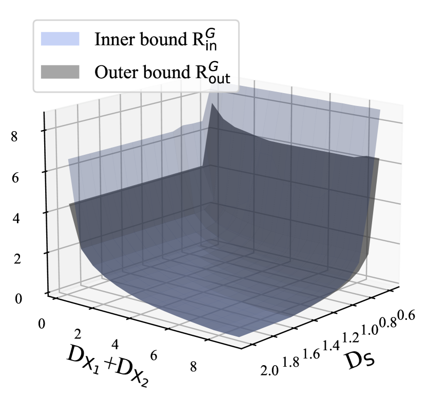
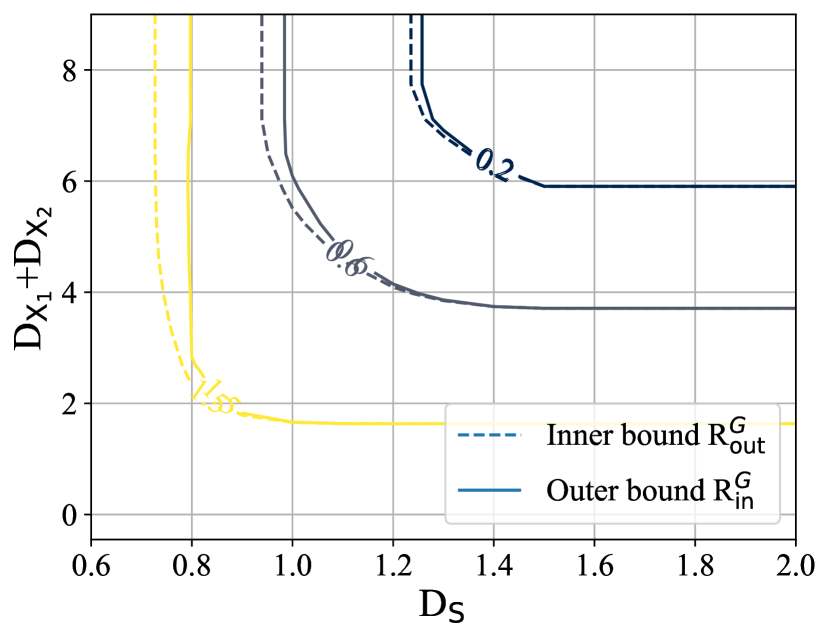
Figure 2: Characterizations for sum rate bounds of a Gaussian semantic-aware 2-links source coding: (a) Illustration for bounds over $D_{S}$ and $D_{X_{1}}+D_{X_{2}}$; (b) The trade-off between two distortions by fixing the sum rate $R_{\mathrm{sum}}=0.2,0.6,1.5$

We further present a toy example for a 2-links Gaussian semantic-aware source coding scenario, in which two observations possess different length $n_{1}=2$ and $n_{2}=1$. The overall covariance matrix ${\textbf{K}}_{\bm{X}}$, MSE matrix ${\textbf{K}}_{Z}$ and estimator $\bm{h}$ are stated as follows, respectively.

$${\textbf{K}}_{\bm{X}}=\begin{bmatrix}6&0&0.125\\ 0&1.5&-0.5\\ 0.125&-0.5&0.38125\end{bmatrix},\quad{\textbf{K}}_{Z}=\begin{bmatrix}0.396&0.090\\ 0.090&0.202\end{bmatrix},\quad\bm{h}=\begin{bmatrix}0.072&0.180&0.541\\ 0.016&0.404&-0.786\end{bmatrix}$$

Fig. 2 illustrates the characterization for sum rate bounds in Theorem 2. In Fig. 2(a), converse bound $R^{G}_{\mathrm{out}}(D_{S},\bm{D}_{X},{\textbf{K}}_{\bm{N}})$ is obtained with alternating minimization by fixing D and $\bm{\Gamma}$ successively via CVXPY, since the constraints involves the inverse of matrix to be optimized. Then the minimum is attained by the search over block diagonal matrix ${\textbf{K}}_{\bm{X}}^{-1}+{\textbf{K}}_{\bm{N}}^{-1}$. In contrast, achievability bound is higher than the converse since the constraint in Eq. (22) is stricter. In Fig. 2(b), the trade-off between two constraints are present by fixing the sum rate. The contour projections show that the constraints on semantic and observations in Eq. (18) and (19) will active simultaneously in multi-user scenarios. More specifically, given two distortions the first user is easy to recover the semantic and hence $\bm{D}_{X}$ is active, while the second user lies in the opposite situation. In the following, we give some degernated cases of Theorem 2.

IV Rate-Distortion function under Logarithmic Distortion

In view of the AI-based frameworks, the quadratic loss always describe the mean square error, which is commonly used in linear regression tasks but restricted in cope with other tasks, e.g. classification. In this section, we study the rate-distortion behavior of the semantic-aware multi-terminal source coding problem with a different distortion measure, namely the logarithmic loss, or we call it cross entropy loss, which is defined as

$$d\left(x,\hat{x}\right)\triangleq\frac{1}{\log\hat{x}(x)},$$ (36)

where $\hat{x}(x)$ denotes the Kullback-Leibler (KL) divergence between the reconstruction $\hat{x}$ and the empirical distribution. Since the convergence via logarithmic loss will not depend on derivative of the sigmoid function, resulting in a fast convergence on loss functions in training progress [31][32]. Therefore, it is valuable to research source coding problem with logarithmic loss.

IV-A Joint Gaussian Distributed Sources with Logarithmic Loss

Theorem 3.

With the same joint Gaussian distributed sources in Theorem 2, and equipped with the logarithmic distortion measures which are defined as $d_{S}(\bm{s},\hat{\bm{s}})=-\log\hat{\bm{s}}(\bm{s})$ and $d_{X}(\bm{x},\hat{\bm{x}})=-\log\hat{\bm{x}}(\bm{x})$. Given $\mathrm{tr}\{{\textbf{K}}_{Z}\}\leq D_{S}\leq\mathrm{tr}\{{\textbf{K}}_{S}\}$, $0\leq D_{X_{i}}\leq\mathrm{tr}\{{{\textbf{K}}}_{X_{i}}\}$, and a positive definite matrix ${\textbf{K}}_{\bm{N}}\in\mathcal{K}({\textbf{K}}_{\bm{X}})$, the sum rate-distortion function $\widetilde{R}^{G}(D_{S},\bm{D}_{X})$ can be bounded by

$$\min_{{\textbf{K}}_{\bm{N}}\in\mathcal{K}({\textbf{K}}_{\bm{X}})}\widetilde{R}^{G}_{\mathrm{out}}(D_{S},\bm{D}_{X},{\textbf{K}}_{N})\leq\widetilde{R}^{G}(D_{S},\bm{D}_{X})\leq\widetilde{R}^{G}_{\mathrm{in}}(D_{S},\bm{D}_{X}),$$ (37)

where

$$\widetilde{R}^{G}_{\mathrm{out}}(D_{S},D_{X},{\textbf{K}}_{N})= \min_{{\textbf{D}},\bm{\Gamma}} \frac{1}{2}\log\frac{\det({\textbf{K}}_{\bm{X}}+{\textbf{K}}_{\bm{N}})\det\left(({\textbf{K}}_{\bm{X}}^{-1}+{\textbf{K}}_{\bm{N}}^{-1})^{-1}\right)}{\det({\textbf{K}}_{\bm{N}})\det\left(\bm{\Gamma}\right)}-\mathrm{tr}\left({\textbf{D}}\right),$$ (38)

s.t. $$\bm{\Gamma}\preceq({\textbf{D}}^{-1}+{\textbf{K}}_{N}^{-1})^{-1},$$ (39)

$$\mathrm{tr}\left\{\bm{h}^{T}{\textbf{D}}\bm{h}+{\textbf{K}}_{Z}\right\}\leq D_{S},$$ (40)

$$\mathrm{tr}\left\{{\textbf{E}}_{i}^{T}{\textbf{D}}{\textbf{E}}_{i}\right\}\leq D_{X_{i}},\text{ for }i=1,2,\cdots,L,$$ (41)

$$\bm{\Gamma}\in\mathcal{K}_{\mathrm{BD}},$$ (42)

and

$$\widetilde{R}^{G}_{\mathrm{in}}(D_{S},\bm{D}_{X})= \min_{{\textbf{D}},\bm{\Gamma}\in\mathbb{R}^{L\times L}} \frac{1}{2}\log\frac{\det({\textbf{K}}_{X}+{\textbf{K}}_{N})\det\left(({\textbf{K}}_{X}^{-1}+{\textbf{K}}_{N}^{-1})^{-1}\right)}{\det({\textbf{K}}_{N})\det\left(\bm{\Gamma}\right)}-\mathrm{tr}\left({\textbf{D}}\right),$$ (43)

s.t. $$\bm{\Gamma}=({\textbf{D}}^{-1}+{\textbf{K}}_{N}^{-1})^{-1},$$ (44)

$$\mathrm{tr}\left\{\bm{h}^{T}{\textbf{D}}\bm{h}+{\textbf{K}}_{Z}\right\}\leq D_{S},$$ (45)

$$\mathrm{tr}\left\{{\textbf{E}}_{i}^{T}{\textbf{D}}{\textbf{E}}_{i}\right\}\leq D_{X_{i}},\text{ for }i=1,2,\cdots,L,$$ (46)

$$\bm{\Gamma}\in\mathcal{K}_{\mathrm{BD}}.$$ (47)

Proof.

See Appendix C. ∎

The proof of Theorem 3 follows similarly with Theorem 2 since the Gaussian nature of sources has not been changed. Specifically, the logarithmic loss brings a different connection between the entropy and the distortions, which will be explained in Lemma 1 in Appendix C and results in the different form of the objective function. Note that the proof technique remains the constraints of outer and inner bounds invariant in comparison with Theorem 2. Next we present a scalar extension with binary sources and loagrithmic loss, which is exactly the mathematic model for classification framework of semantic-aware compression.

IV-B Binary Memoryless Sources with Logarithmic Loss

In this subsection, we introduce outer and inner bounds of sum rate for semantic-aware MT source coding, where the semantic source and observations are all Bernoulli-distributed and logarithmic loss is adopted. Different from the Gaussian case, the estimator for semantic reconstruction in Bernoulli case highly depends on how to decide the output of a binary sequence. Therefore, two bounds relying on different decision rules are presented in the following.

Theorem 4.

Let $S$ be a Bernoulli source which takes values from a binary set with equal probability. The $i$-th noisy observation $X_{1},X_{2},\cdots,X_{L}$ is $X_{i}=S+N_{i}$, where $N_{i}$ is generated from the Bernoulli source with crossover probability $p_{i}$, i.e. $N_{i}\sim\mathrm{Ber}(p_{i})$ for $i=1,2,\cdots,L$. Given the logarithmic distortion measure, the sum rate-distortion function $\widetilde{R}^{B}(D_{S},\bm{D}_{X})$ can be bounded by

$$\widetilde{R}^{B}_{\mathrm{out}}(D_{S},\bm{D}_{X})\leq\widetilde{R}^{B}(D_{S},\bm{D}_{X})\leq\widetilde{R}^{B}_{\mathrm{in}}(D_{S},\bm{D}_{X})$$

where

$$\widetilde{R}^{B}_{\mathrm{out}}(D_{S},\bm{D}_{X})= \min_{d_{1},d_{2},\cdots,d_{L}} \Phi\left(\left\{p_{1},p_{2},\cdots,p_{L}\right\}\right)-\sum_{i=1}^{L}d_{i},$$ (48)

$$\mathrm{s.t.} \Phi\left(\left\{0,\alpha_{1},\alpha_{2},\cdots,\alpha_{L}\right\}\right)-\Phi\left(\left\{\alpha_{1},\alpha_{2},\cdots,\alpha_{L}\right\}\right)\leq D_{S},$$ (49)

$$0\leq d_{i}\leq D_{X_{i}},\text{ for }i=1,2,\cdots,L,$$ (50)

and

$$\widetilde{R}^{B}_{\mathrm{in}}(D_{S},\bm{D}_{X})= \min_{d_{1},d_{2},\cdots,d_{L}} \Phi\left(\left\{p_{1},p_{2},\cdots,p_{L}\right\}\right)-\sum_{i=1}^{L}d_{i},$$ (51)

$$\mathrm{s.t.} \mathcal{G}(\alpha_{1},\alpha_{2},\cdots,\alpha_{L})\leq D_{S},\hskip 142.26378pt$$ (52)

$$0\leq d_{i}\leq D_{X_{i}}\text{ for }i=1,2,\cdots,L,$$ (53)

Here $\alpha_{i}=p_{i}*H^{-1}(d_{i})$ and the joint entropy $\Phi(\mathcal{A})$ of set $\mathcal{A}$ is stated as:

$$\Phi(\mathcal{A})=-\sum_{i=1}^{2^{(|\mathcal{A}|)}}q_{i}\log_{2}\left(q_{i}\right),$$ (54)

where

$$q_{i}=\frac{1}{2}\left(\prod_{j\in\mathcal{B}_{i}}p_{j}\prod_{\ell\in\mathcal{B}_{i}^{c}}\bar{p}_{\ell}+\prod_{j\in\mathcal{B}_{i}}\bar{p}_{j}\prod_{\ell\in\mathcal{B}_{i}^{c}}p_{\ell}\right).$$

with $\bar{p}=$ $1-p$ and $\mathcal{B}_{i}\subseteq\{1,\cdots,|\mathcal{A}|\}$. Moreover,

$$\mathcal{G}(\alpha_{1},\alpha_{2},\cdots,\alpha_{L})=\left\{\begin{aligned} \sum_{t=(L+1)/2}^{L}\mathbb{P}\{T=t\}&&L\text{ is odd},\\ \frac{1}{2}\mathbb{P}\left\{T=L/2\right\}+\sum_{t=(L+1)/2}^{L}\mathbb{P}\{T=t\}&&L\text{ is even}.\end{aligned}\right.$$ (55)

where

$$\mathbb{P}\{T=t\}=\sum_{\mathcal{B}_{j}\in\mathcal{Q}_{t}}\prod_{j\in\mathcal{B}_{i}}\alpha_{j}\prod_{\ell\in\mathcal{B}_{i}^{c}}\bar{\alpha_{1}}_{\ell}$$

Proof.

See Appendix D. ∎

V Conclusion

In this paper, we investigate upper and lower bounds of semantic-aware MT source coding problem. Based on the general model, the case when the sources are Gaussian distributed under a quadratic distortion are studied. By exposing the linear relationship between semantic and observations in the Gaussian case, we characterize the sum rate region via the LMMSE estimator. The tradeoff between two distortions can be express explicitly through the statements and the plots. Moreover, the degenerated cases to existing works are presented. To characterize the practical compression model with specific tasks, we further explore the case under Bernoulli sources and logarithmic loss.

In future works, we aim to analyze the more complicated model, e.g. the side information related to Wyner-Ziv source coding problem[33],[34], in which the side information is exactly the semantic knowledge bases at encoders and decoder. Besides, the finite block length analysis for semantic-aware compression [27] will also be taken into consideration for practical application.

Appendix A Proof of Theorem 2

In this appendix we present the proof of upper and lower bounds of the sum rate-distortion function in a Gaussian semantic-aware multi-terminal source coding problem. The proof mainly follows Wang et al. [18], in which the authors provide a new method based on estimation-theoretic tool instead of the entropy power inequality (EPI) to characterize the multi-terminal source coding problem. Compared with their model, since we have an extra constraint on the semantic source, we provide the proof of converse and achievability bounds for completeness.

A-A Converse

The overview of the proof is the following. Under the Gaussian setups, we start from an additional random vector $\bm{Y}_{\mathcal{L}}=\{\bm{Y}_{1},\bm{Y}_{2},\cdots,\bm{Y}_{L}\}=\{\bm{X}_{1}+\bm{N}_{1},\bm{X}_{2}+\bm{N}_{2},\cdots,\bm{X}_{L}+\bm{N}_{L}\}$, where $\bm{N}_{\mathcal{L}}=\{\bm{N}_{1},\bm{N}_{2},\cdots,\bm{N}_{L}\}$ with covariance matrix ${\textbf{K}}_{\bm{N}}$ are independent with $\bm{X}_{\mathcal{L}}$. Note that we select the noise vector $\bm{N}$ such that $\{\bm{X}_{1},\bm{X}_{2},\cdots,\bm{X}_{L}\}$ are independent given $\bm{Y}_{\mathcal{L}}$, which is equivalent to that ${\textbf{K}}_{\bm{X}}^{-1}+{\textbf{K}}_{\bm{N}}^{-1}$ is a diagonal matrix. This assumption enables us split the mutual information as the main component and the $L$ branches in multi-terminal source problem as in the CEO problem. Next, different estimators are built via vectors $\bm{Y}_{\mathcal{L}},\bm{X}_{\mathcal{L}}$ and codewords $C_{\mathcal{L}}$. Then connections between different estimates are constructed due to the fact that linear minimum mean square error (LMMSE) estimator is always worse than minimum mean square error (MMSE) estimator, and finally the converse bound is obtained. For further use, we define MMSE matrix ${\textbf{D}}_{\bm{X}_{\mathcal{L}}|c_{\mathcal{L}}}\triangleq\mathbb{E}[\bm{X}_{\mathcal{L}}-\mathbb{E}[\bm{X}_{\mathcal{L}}|c_{\mathcal{L}}]][\bm{X}_{\mathcal{L}}-\mathbb{E}[\bm{X}|c_{\mathcal{L}}]]^{T}$.

We first lower bound the sum rate as

$$\sum_{i=1}^{L}\log|\mathcal{C}_{i}|\geq H\left(C_{\mathcal{L}}\right) =I(\bm{X}_{\mathcal{L}}^{k};C_{\mathcal{L}})$$ (56)

$$\overset{(a)}{=}I\left(\bm{X}_{\mathcal{L}}^{k},\bm{Y}_{\mathcal{L}}^{k};C_{\mathcal{L}}\right)$$ (57)

$$\overset{(b)}{=}I\left(\bm{Y}_{\mathcal{L}}^{k};C_{\mathcal{L}}\right)+\sum_{i=1}^{L}I\left(X_{i}^{k};C_{i}\mid\bm{Y}_{\mathcal{L}}^{k}\right)$$ (58)

$$=h(\bm{Y}_{\mathcal{L}}^{k})-h\left(\bm{Y}_{\mathcal{L}}^{k}\mid C_{\mathcal{L}}\right)+\sum_{i=1}^{L}\left(h\left(X_{i}^{k}\mid\bm{Y}_{\mathcal{L}}^{k}\right)-h\left(X_{i}^{k}\mid\bm{Y}_{\mathcal{L}}^{k},C_{i}\right)\right).$$ (59)

where $(a)$ follows the Markov chain $\bm{Y}_{\mathcal{L}}^{k}-\bm{X}_{\mathcal{L}}^{k}-C_{\mathcal{L}}$ and $(b)$ follows the Markov chain $C_{i}-X_{i}^{k}-\bm{Y}_{\mathcal{L}}^{k}-X_{j}^{k}-C_{j}$ where $i\neq j$. We further define two MSE estimators as

$${\textbf{D}}\triangleq\mathbb{E}[\bm{X}^{k}_{\mathcal{L}}-\mathbb{E}[\bm{X}_{\mathcal{L}}^{k}|C_{\mathcal{L}}]][\bm{X}_{\mathcal{L}}^{k}-\mathbb{E}[\bm{X}_{\mathcal{L}}^{k}|C_{\mathcal{L}}]]^{T}={\textbf{D}}_{\bm{X}^{k}|C_{\mathcal{L}}},$$ (60)

$$\bm{\Gamma}\triangleq\mathbb{E}[\bm{X}_{\mathcal{L}}^{k}-\mathbb{E}[\bm{X}_{\mathcal{L}}^{k}|\bm{Y}_{\mathcal{L}}^{k},C_{\mathcal{L}}]][\bm{X}^{k}-\mathbb{E}[\bm{X}_{\mathcal{L}}^{k}|\bm{Y}_{\mathcal{L}}^{k},C_{\mathcal{L}}]]^{T}={\textbf{D}}_{\bm{X}_{\mathcal{L}}^{k}|\bm{Y}_{\mathcal{L}}^{k},C_{\mathcal{L}}}.$$ (61)

It is easy to verify that

$$\mathbb{E}[X_{i}^{k}-\mathbb{E}[X_{i}^{k}|\bm{Y}_{\mathcal{L}}^{k},C_{\mathcal{L}}]][X_{j}^{k}-\mathbb{E}[X_{j}^{k}|\bm{Y}_{\mathcal{L}}^{k},C_{\mathcal{L}}]]^{T}=0$$ (62)

when $i\neq j$. Therefore $\bm{\Gamma}$ is a block diagonal matrix, yielding

$$\sum_{i=1}^{L}h\left(X_{i}^{k}\mid\bm{Y}_{\mathcal{L}}^{k},C_{i}\right)=\frac{1}{2}\log\det\left(\bm{\Gamma}\right)$$ (63)

Next, we consider $\bm{C}=\mathbb{E}[\bm{X}_{\mathcal{L}}^{k}|C_{\mathcal{L}}]$, the covariance matrix among three random vectors can be stated as

$${\textbf{K}}_{\left(\mathbf{X}_{\mathcal{L}}^{T},\mathbf{Y}_{\mathcal{L}}^{T},\mathbf{W}^{T}\right)^{T}}=\left(\begin{array}[]{ccc}{\textbf{K}}_{\bm{X}}&{\textbf{K}}_{\bm{X}}&{\textbf{K}}_{\bm{X}}-\mathbf{D}\\ {\textbf{K}}_{\bm{X}}&{\textbf{K}}_{\bm{X}}+{\textbf{K}}_{\bm{N}}&{\textbf{K}}_{\bm{X}}-\mathbf{D}\\ {\textbf{K}}_{\bm{X}}-\mathbf{D}&{\textbf{K}}_{\bm{X}}-\mathbf{D}&{\textbf{K}}_{\bm{X}}-\mathbf{D}\end{array}\right)$$ (67)

and hence we compute the LMMSE ${\textbf{D}}^{\mathrm{LM}}_{\bm{X}_{\mathcal{L}}^{k}|\bm{Y}_{\mathcal{L}}^{k},\bm{C}}$ as

$${\textbf{D}}^{\mathrm{LM}}_{\bm{X}_{\mathcal{L}}^{k}|\bm{Y}_{\mathcal{L}}^{k},\bm{C}} ={\textbf{K}}_{\bm{X}}-{\textbf{K}}_{\bm{X}_{\mathcal{L}}^{k},(\bm{Y}_{\mathcal{L}}^{k},\bm{C}^{k})}{\textbf{K}}^{-1}_{(\bm{Y}_{\mathcal{L}}^{k},\bm{C}^{k})}{\textbf{K}}^{T}_{\bm{X}_{\mathcal{L}}^{k},(\bm{Y}_{\mathcal{L}}^{k},\bm{C}^{k})}=\left({\textbf{D}}^{-1}+{\textbf{K}}_{\bm{N}}^{-1}\right)^{-1}$$ (68)

The constrain Eq. (17) follows the fact

$${\textbf{D}}_{\bm{X}_{\mathcal{L}}^{k}|\bm{Y}_{\mathcal{L}}^{k},C_{\mathcal{L}}}\leq{\textbf{D}}_{\bm{X}_{\mathcal{L}}^{k}|\bm{Y}_{\mathcal{L}}^{k},\bm{C}}\leq{\textbf{D}}^{\mathrm{LM}}_{\bm{X}_{\mathcal{L}}^{k}|\bm{Y}_{\mathcal{L}}^{k},\bm{C}}$$ (69)

Now we include the semantic distortion $d(S,\hat{S})\leq D_{S}$ into the multi-terminal source coding problem, which in fact is a surrogate distortion measure [27, p. 79] [26]. That is to say, the semantic distortion constraint for $S$ can be converted to a surrogate distortion constraint for ${\textbf{X}}_{\mathcal{L}}$. Given a matrix $\bm{h}\in\mathbb{R}^{m\times\sum_{i}^{L}n_{i}}$ and a Gaussian noise $\bm{Z}$ with covariance matrix ${\textbf{K}}_{Z}$, we write ${\textbf{S}}=\bm{h}\bm{X}_{\mathcal{L}}+\bm{Z}$. Note that $\bm{Z}$ is independent with $\bm{X}_{\mathcal{L}}$. Hence the semantic distortion constraint can be rewritten as

$$\mathbb{E}d_{S}\left(\bm{S},\hat{\bm{S}}\right) =\mathrm{tr}\left\{\mathbb{E}[\bm{S}-\mathbb{E}[\bm{S}|C_{\mathcal{L}}]][\bm{S}-\mathbb{E}[\bm{S}|C_{\mathcal{L}}]]^{T}\right\}$$ (70)

$$=\mathrm{tr}\left\{\mathbb{E}[\bm{h}\bm{X}_{\mathcal{L}}+\bm{Z}-\mathbb{E}[\bm{h}\bm{X}_{\mathcal{L}}+\bm{Z}|C_{\mathcal{L}}]][\bm{h}\bm{X}_{\mathcal{L}}+\bm{Z}-\mathbb{E}[\bm{h}\bm{X}_{\mathcal{L}}+\bm{Z}|C_{\mathcal{L}}]]^{T}\right\}$$ (71)

$$=\mathrm{tr}\left\{\bm{h}\mathbb{E}[\bm{X}_{\mathcal{L}}-\mathbb{E}[\bm{X}_{\mathcal{L}}|C_{\mathcal{L}}]]\mathbb{E}[\bm{X}_{\mathcal{L}}-\mathbb{E}[\bm{X}_{\mathcal{L}}|C_{\mathcal{L}}]]^{T}\bm{h}^{T}+\mathbb{E}\bm{Z}\bm{Z}^{T}\right\}$$ (72)

$$=\mathrm{tr}\left\{\bm{h}{\textbf{D}}\bm{h}^{T}+{\textbf{K}}_{Z}\right\}\leq D_{S}$$ (73)

which yields the constraint Eq. (18). Therefore the converse bound $R^{G}_{\mathrm{out}}(D_{S},\bm{D}_{X},{\textbf{K}}_{N})$ is stated as an optimization problem with constraints Eq. (17)- Eq. (19) in Theorem 2.

A-B Achievability

The achievability proof simply follows the Berger-Tung inner bound for multi-terminal source coding[26] with an extra semantic source constraint. The upper bound on sum rate distortion is obtained by proper Gaussian auxiliary random vectors and the fact the LMMSE estimator coincides MMSE estimator under Gaussian setups. More specifically, we write the Berger-Tung inner bound of sum rate for $L$-terminals

$$\sum_{i=1}^{L}R_{i} \geq I(\bm{X}^{k};\bm{U}^{k})$$ (74)

$$=I(\bm{Y}^{k},\bm{X}^{k};\bm{U}^{k})$$ (75)

$$=I(\bm{Y}^{k};\bm{U}^{k})+\sum_{i=1}^{L}I(X_{i}^{k};U_{i}^{k}|\bm{Y}^{k})$$ (76)

where $\bm{Y}^{k}$ is the imaginary remote source and $\bm{U}=\{U_{1},U_{2},\cdots,U_{L}\}$ with $U_{i}=X_{i}+W_{i}$ for $i=1,2,\cdots,L$. Equipped with ${\textbf{D}}={\textbf{D}}_{\bm{X}^{k}|{\textbf{U}}_{\mathcal{L}}}$, $\bm{\Gamma}={\textbf{D}}_{\bm{X}^{k}|\bm{Y}^{k},{\textbf{U}}_{\mathcal{L}}}$ and $\widetilde{{\textbf{U}}}=\mathbb{E}[\bm{X}|{\textbf{U}}_{\mathcal{L}}]$, now it is enough to show

$$\bm{\Gamma} ={\textbf{D}}_{\bm{X}^{k}|\bm{Y}^{k},{\textbf{U}}_{\mathcal{L}}}={\textbf{D}}_{\bm{X}^{k}|\bm{Y}^{k},\widetilde{{\textbf{U}}}}={\textbf{D}}^{\mathrm{LM}}_{\bm{X}^{k}|\bm{Y}^{k},\widetilde{{\textbf{U}}}}=\left({\textbf{D}}^{-1}+{\textbf{K}}_{N}^{-1}\right)^{-1}.$$ (77)

Moreover, with the surrogate constraint argument we obtain $\bm{h}{\textbf{D}}\bm{h}^{T}+\sigma_{Z}^{2}\leq D_{S}$ and the achievability bound $R^{G}_{\mathrm{in}}(D_{S},\bm{D}_{X})$.

Appendix B Proof of Corollary 1

We provide the proofs of these degenerated cases in this appendix.

1. (Gaussian Semantic-aware single use rate-distortion function) The multi-terminal source coding problem is reduced to the single use source coding problem given $L=1$, in which the rate-distortion function can be characterized explicitly. It means that the outer bound in Eq. (16) coincides the inner bound in Eq. (21) and we immediately obtain the rate-distortion characterization of semantic-aware source coding with constraints $\mathrm{tr}\left\{\bm{h}{\textbf{D}}\bm{h}^{T}+{\textbf{K}}_{Z}\right\}\leq D_{S}$ and $\mathrm{tr}\left\{{\textbf{D}}\right\}\leq D_{X}$ as

   $$R^{G}_{\mathrm{out}}(D_{S},\bm{D}_{X},{\textbf{K}}_{N})=R^{G}_{\mathrm{in}}(D_{S},\bm{D}_{X})=\min_{{\textbf{D}}}\frac{1}{2}\log\left(\frac{\det({\textbf{K}}_{\bm{X}})}{\det({\textbf{D}})}\right)$$ (78)

   according to Prop. 1, where constraint Eq. (29) is removed since ${\textbf{D}}^{-1}-{\textbf{K}}_{\bm{X}}^{-1}$ reduces to a scalar. This is the semantic rate-distortion function in [12, Theorem 2].

2. (Asymmetric Gaussian CEO problem) It is natural to remove constraints Eq. (17) and Eq. (19), since with the assumption that $\bm{D}_{X}\rightarrow\infty$, we get

   $$\bm{\Gamma}\preceq\left({\textbf{K}}_{X}^{-1}+{\textbf{K}}_{N}^{-1}\right)^{-1}\preceq\left({\textbf{D}}^{-1}+{\textbf{K}}_{N}^{-1}\right)^{-1}$$ (79)

   Now equipped with slightly different notations that $X=S+W_{i}$, where $W_{i}\sim\mathcal{N}(0,\sigma_{W_{i}}^{2})$ and $\gamma_{i}$ is the $i$-th diagonal entry of D, Eq. (18) can be readily rewritten as

   $$\bm{h}{\textbf{D}}\bm{h}^{T}+\sigma_{Z}^{2}=\sum_{i=1}^{L}\frac{\sigma_{Z}^{4}}{\sigma_{W_{i}}^{4}}\gamma_{i}+\sigma_{Z}^{2}\leq D_{S}$$ (80)

   where $\sigma_{Z}^{2}=\left(\sigma_{S}^{-2}+\sum_{i=1}^{L}\sigma^{-2}_{W_{i}}\right)^{-1}$ and $\bm{h}=\sigma_{Z}^{2}[\sigma_{W_{1}}^{-2},\sigma_{W_{2}}^{-2},\cdots,\sigma_{W_{L}}^{-2}]$. Then the bounds in [18, Problem 1,Problem 2] are able to obtained by dividing $\sigma_{Z}^{2}D_{S}$ at each side of the constraint Eq. (80).

3. (Symmetric Gaussian CEO problem) Obviously this is a special case of asymmetric Gaussian CEO problem. By assuming the covariance matrix of $\bm{X}$ is an identity matrix ${\textbf{I}}_{L}$, and consequently equal distortions constraints $\bm{D}_{X}=\bm{1}_{L}$, we can acquire the explicit characterization of rate-distortion function same as Oohamma [16, Theorem 1].

4. (Asymmetric MT source coding problem) The degeneration of the case $D_{s}\rightarrow\infty$ can be attained directly by removing the constraint in Eq. (18) and Eq. (23). Then Theorem 2 coincides the bounds in [18, Theorem 1,Theorem 2].

5. (2-links MT source coding problem) The degeneration of the case $D_{s}\rightarrow\infty$ and $L=2$ is obtained by selecting

   $${\textbf{K}}_{N}=\left(\begin{array}[]{cc}d_{1}&-\theta\sqrt{d_{1}d_{2}}\\ -\theta\sqrt{d_{1}d_{2}}&d_{2}\end{array}\right)\in\mathcal{K}\left({\textbf{K}}_{X}\right)$$ (83)

   where

   $$\theta=\frac{\sqrt{\left(1-\rho^{2}\right)^{2}+4\rho^{2}d_{1}d_{2}}-\left(1-\rho^{2}\right)}{2\rho\sqrt{d_{1}d_{2}}}$$

   and $\rho=\mathbb{E}[X_{1}X_{2}]$. The following derivation is present in [16, Theorem 1] by combining a two-link source coding problem with a CEO problem. For more details, reader can turn to [18, Theorem 6].

Appendix C Proof of Theorem 3

The proof of Theorem 3 mainly follows Theorem 2 since the nature of Gaussian random variables remains invariant. However, equipped with the logarithmic distortion, it is necessary to first expose the connection between the entropy and the distortion, which can be stated as $h(\bm{X}|\hat{\bm{X}})\leq\frac{1}{2}\log(2\pi e)\det({\textbf{D}}_{\bm{X}|\hat{\bm{X}}})$ in quadratic distortion measure under Gaussian case. The following lemma reveals the above issue as

Lemma 1.

c.f. [35, Lemma 1] Let $\hat{\bm{X}_{\mathcal{L}}^{k}}=\psi_{S}(C_{\mathcal{L}})$ be the argument of the recovered observations, and $d(\bm{s},\hat{\bm{s}})=\log\frac{1}{\hat{\bm{s}}(\bm{s})}$, then

$$\mathbb{E}d\left(\bm{S}^{k},\hat{\bm{S}}^{k}\right)\geq h(\bm{S}^{k}|\hat{\bm{X}_{\mathcal{L}}^{k}})$$ (84)

Lemma 1 enables us upper bound the conditional entropy as

$$h\left(\bm{Y}_{\mathcal{L}}^{k}\mid C_{\mathcal{L}}\right) =h\left(\bm{X}_{\mathcal{L}}^{k}+\bm{N}_{\mathcal{L}}^{k}\mid C_{\mathcal{L}}\right)$$ (85)

$$\leq\sum_{i=1}^{L}h\left(\bm{X}_{i}^{k}\mid C_{\mathcal{L}}\right)$$ (86)

$$\leq\sum_{i=1}^{L}\mathbb{E}_{\bm{X}_{i}^{k}|c_{\mathcal{L}}}d^{k}_{X}\left(\bm{X}_{i}^{k},\hat{\bm{X}_{i}}^{k}\right)$$ (87)

$$\leq\mathrm{tr}({\textbf{D}}),$$ (88)

which implies that

$$\sum_{i=1}^{L}\log|\mathcal{C}_{i}|\geq\frac{1}{2}\log\frac{\det({\textbf{K}}_{X}+{\textbf{K}}_{N})\det\left(({\textbf{K}}_{X}^{-1}+{\textbf{K}}_{N}^{-1})^{-1}\right)}{\det({\textbf{K}}_{N})\det\left(\bm{\Gamma}\right)}-\mathrm{tr}\left({\textbf{D}}\right),$$ (89)

if following the same steps in Theorem 2, and hence completes the proof of Theorem 3.

Appendix D Proof of Theorem 4

Herein we provide the proof of the rate-distortion function with Bernoulli sources $(S,X_{1},X_{2},$ $\cdots,X_{L})$ under the semantic-aware multi-terminal source coding framework. Now consider $S\sim\mathrm{Ber}(\frac{1}{2})$ and $\mathbb{P}(x_{i}\neq S)=p_{i}$ for $i=1,2,\cdots,L$, and the logarithmic distortion measure, the outline of the proof is the following.

D-A Converse

For the converse proof, the first part is similar as the regular multi-terminal source coding problem with binary source [36], in which we obtain the sum-rate distortion function characterized via the binary joint entropy expression $\Phi$. Like the Gaussian case, the estimated semantic source $\hat{S}$ can be obtained by reconstructed observations $\hat{X}_{1},\hat{X}_{2},\cdots,\hat{X}_{L}$ via different decision rules. In the second part, we introduce the optimal decision rules according to the normal rate-distortion function, and formulate the converse bound as an optimization problem.

We first consider

$$k\sum_{i=1}^{L}R_{i} \geq\sum_{i}^{L}H(C_{i})\geq H(C_{\mathcal{L}})$$ (90)

$$=I(X_{1}^{k},X_{2}^{k}\cdots,X_{L}^{k};C_{\mathcal{L}})$$ (91)

$$=I(X_{1}^{k};C_{\mathcal{L}})+I(X_{2}^{k},\cdots,X_{L}^{k};C_{\mathcal{L}}|X_{1}^{k})$$ (92)

$$\geq I(X_{1}^{k},\hat{X}_{1}^{k})+I(X_{2}^{k},\cdots,X_{L}^{k}:C_{\mathcal{L}},X_{1}^{k})-I(X_{2}^{k},\cdots,X_{L}^{k};X_{1}^{k})$$ (93)

$$\geq\sum_{i=1}^{L}\left(I(X_{i}^{k},\hat{X}_{i}^{k})-I(X_{i}^{k};X_{i+1}^{k},\cdots,X_{L}^{k})\right)$$ (94)

It can be readily verified with Lemma 1.

$$\frac{1}{k}I(X_{i}^{k},\hat{X}_{i}^{k}) =I(X_{i},\hat{X}_{i})=H(X_{i})-H(X_{i}|\hat{X}_{i})\geq H(p_{i})-\mathbb{E}d\left[X_{i};\hat{X}_{i}\right]$$ (95)

and

$$\frac{1}{k}\sum_{i=1}^{L}\left(I(X_{i}^{k};X_{i+1}^{k},\cdots,X_{L}^{k})\right) =H(X_{1},X_{2}\cdots,X_{L})-\sum_{i=1}^{L}H(X_{i})$$ (96)

$$=\Phi\left(\left\{p_{1},p_{2},\cdots,p_{L}\right\}\right)-\sum_{i=1}^{L}H(p_{i})$$ (97)

By denoting $d_{i}=\mathbb{E}d\left[X_{i},\hat{X}_{i}\right]$ for $i=1,2,\cdots,L$ and substituting Eq. (95) and Eq. (97) in Eq. (94), we obtain the sum rate-distortion bound as Eq. (48), and the constraints on $di$ as shown in in Eq. (94) follow immediately.

Now it is left to show the relationship between the observations and the semantic distortion $D_{S}$. We clarify that the rate-distortion performance for such a binary multi-terminal source coding problem largely depends on the decision rule at the decoder, when given the recovered $\hat{X}_{1},\hat{X}_{2},\cdots,\hat{X}_{L}$. The optimal decision rule can be formulated according to the original rate-distortion function of the semantic source as:

$$\frac{1}{k}\left(H(S^{k})-kD_{S}\right) =\frac{1}{k}\left(H(S^{k})-H(S^{k}|\hat{S}^{k})\right)$$ (98)

$$=\frac{1}{k}I(S^{k};\hat{S}^{k})$$ (99)

$$\leq I\left(S;\hat{X}_{1},\hat{X}_{2},\cdots,\hat{X}_{L}\right)$$ (100)

$$=H(S)+H\left(\hat{X}_{1},\hat{X}_{2},\cdots,\hat{X}_{L}\right)-H\left(S,\hat{X}_{1},\hat{X}_{2},\cdots,\hat{X}_{L}\right)$$ (101)

$$=H(S)+\Phi\left(\left\{\alpha_{1},\alpha_{2},\cdots,\alpha_{L}\right\}\right)-\Phi\left(\left\{0,\alpha_{1},\alpha_{2},\cdots,\alpha_{L}\right\}\right),$$ (102)

where $\hat{X}_{i}$ can be treated as a Bernoulli random variable with crossover probability $\alpha_{i}=p_{i}*H^{-1}(d_{i})$ for $i=1,2,\cdots,L$. Owing to the monotonicity of the inverse binary entropy function $H^{-1}(\cdot)$, we obtain the constrain Eq. (49) and complete the converse proof.

D-B Achievability

Since the bound for Bernoulli sources is based on the decision rule, we provide the achievability bound with the majority voting, which means that we output the $0$ or $1$ if they are more than half. In fact, the expectation on semantic distortion is equal to the error probability of judging the received binary sequence falsely. This is a Poisson binomial process [37] hence motivates we define the distortion function $\mathcal{G}(\alpha_{1},\alpha_{2},\cdots,\alpha_{L})$ as Eq. (55). The computation on Poisson binomial functions can be numerically solved by recursive equations or discrete Fourier transform [38].

References

• [1] C. E. Shannon, “A mathematical theory of communication,” Bell Syst. Tech. J., vol. 27, no. 3, pp. 379–423, Jul. 1948.
• [2] R. Carnap and Y. Bar-Hillel, “An outline of a theory of semantic information,” Brit. J. Philosophy Sci., vol. 4, no. 14, pp. 147–157, Oct. 1953.
• [3] J. Bao, P. Basu, M. Dean, C. Partridge, A. Swami, W. Leland, and J. A. Hendler, “Towards a theory of semantic communication,” in Proc. IEEE Netw. Sci. Workshop 2021, Jun. 2011, pp. 110–117.
• [4] B. Guler, A. Yener, and A. Swami, “The semantic communication game,” in IEEE Trans. Cogn. Commun. Netw., Dec. 2018.
• [5] N. Farsad, M. Rao, and A. Goldsmith, “Deep learning for joint source-channel coding of text,” in Proc IEEE Int. Conf. Acoust. Speech Signal Process., (ICASSP), Calgary, AB, Canada, Apr. 2018, pp. 2326–2330.
• [6] H. Xie, Z. Qin, G. Y. Li, and B. Juang, “Deep learning enabled semantic communication systems,” IEEE Trans. Signal Process., vol. 69, pp. 2663–2675, Apr. 2021.
• [7] Z. Weng and Z. Qin, “Semantic communication systems for speech transmission,” IEEE J. Sel. Areas Commun., vol. 39, no. 8, pp. 2434–2444, Jun. 2021.
• [8] M. Kountouris and N. Pappas, “Semantics-empowered communication for networked intelligent systems,” IEEE Commun. Mag., vol. 59, no. 6, pp. 96–102, Jun. 2021.
• [9] D. Huang, X. Tao, F. Gao, and J. Lu, “Deep learning-based image semantic coding for semantic communications,” in IEEE Glob. Commun. Conf. (GLOBECOM), Madrid, Spain, Dec. 2021, pp. 1–6.
• [10] J. Dommel, Z. Utkovski, O. Simeone, and S. Stanczak, “Joint source-channel coding for semantics-aware grant-free radio access in IoT fog networks,” IEEE Signal Process. Lett., vol. 28, pp. 728–732, Apr. 2021.
• [11] P. Jiang, C. Wen, S. Jin, and G. Y. Li, “Deep source-channel coding for sentence semantic transmission with HARQ,” IEEE Trans. Commun., vol. 70, no. 8, pp. 5225–5240, Jun. 2022.
• [12] J. Liu, S. Shao, W. Zhang, and H. V. Poor, “An indirect rate-distortion characterization for semantic sources: General model and the case of Gaussian observation,” IEEE Trans. Commun., Jun. 2022.
• [13] Y. Shi, S. Shao, Y. Wu, W. Zhang, X.-G. Xia, and C. Xiao, “Excess distortion exponent analysis for semantic-aware mimo communication systems,” IEEE Trans. Wireless Commun., 2023(early access).
• [14] F. Liu, W. Tong, Z. Sun, and C. Guo, “Task-oriented semantic communication systems based on extended rate-distortion theory,” Feb. 2022, arxiv: 2201.10929. [Online]. Available: https://arxiv.org/abs/2201.10929
• [15] T. Berger and R. Yeung, “Multiterminal source encoding with one distortion criterion,” IEEE Trans. Inf. Theory, vol. 35, no. 2, p. 228–236, Mar. 1989.
• [16] Y. Oohama, “The rate-distortion function for the quadratic Gaussian CEO problem,” IEEE Trans. Inf. Theory, vol. 44, no. 3, p. 1057–1070, May 1998.
• [17] A. Wagner and V. Anantharam, “An improved outer bound for multiterminal source coding,” IEEE Trans. Inf. Theory, vol. 54, no. 5, p. 1919–1937, May 2008.
• [18] J. Wang, J. Chen, and X. Wu, “On the sum rate of Gaussian multiterminal source coding: New proofs and results,” IEEE Trans. Inf. Theory, vol. 56, no. 8, pp. 3946–3960, Aug. 2010.
• [19] Y. Oohama, “Gaussian multiterminal source coding,” IEEE Trans. Inf. Theory, vol. 43, no. 6, p. 1912–1923, Nov. 1997.
• [20] H. Viswanathan and T. Berger, “The quadratic Gaussian CEO problem,” IEEE Trans. Inf. Theory, vol. 43, no. 5, p. 1549–1559, Sep. 1997.
• [21] Y. Yang and Z. Xiong, “On the generalized Gaussian CEO problem,” IEEE Trans. Inf. Theory, vol. 58, no. 6, p. 3350–3372, Jun. 2012.
• [22] T. Berger, Z. Zhang, and H. Viswanathan, “The CEO problem [multiterminal source coding],” IEEE Trans. Inf. Theory, May 1996.
• [23] S. Tavildar and P. Viswanath, “On the sum-rate of the vector Gaussian CEO problem,” in Proc. Conf. Rec. 39th Asilomar Conf. Signals, Syst. Comput, 2005, Pacific Grove, CA, USA, Oct. 2005, p. 3–7.
• [24] J. Chen and J. Wang, “On the vector Gaussian CEO problem,” in IEEE Int. Symp. Inf. Theory (ISIT) 2011, St. Petersburg, Russia, Jul. 2011, p. 2050–2054.
• [25] E. Ekrem and S. Ulukus, “An outer bound for the vector Gaussian CEO problem,” IEEE Trans. Inf. Theory, vol. 60, no. 11, p. 6870–6887, Nov. 2014.
• [26] T. Berger, Rate-Distortion Theory.   Prentice-Hall, Englewood Cliffs, NJ,, 1971.
• [27] V. Kostina and S. Verdú, “Nonasymptotic noisy lossy source coding,” IEEE Trans. Inf. Theory, Nov. 2016.
• [28] T. Yuan, L. Guo, Y. Yichao, Z. Guangtao, C. Li, and G. Zhiyong, “A coding framework and benchmark towards compressed video understanding,” Jun. 2022, arXiv:2202.02813. [Online]. Available: https://arxiv.org/abs/2202.02813.
• [29] K. Liu, D. Liu, L. Li, N. Yan, and H. Li, “Semantics-to-signal scalable image compression with learned revertible representations,” Int. J. Comput. Vis., vol. 129, no. 9, p. 2605–2621, Sep. 2021.
• [30] A. El Gamal and Y.-H. Kim, Network Information Theory.   Cambridge University Press, 2011.
• [31] Q. Wang, Y. Ma, K. Zhao, and Y. Tian, “A comprehensive survey of loss functions in machine learning,” Ann. Appl. Stat., vol. 9, Apr. 2022.
• [32] C. Lorenzo, E. Adam, L. Marco, M. Ashraf, and R. Alessandro, “A survey and taxonomy of loss functions in machine learning,” Jan. 2023, arXiv:2301.05579. [Online]. Available: https://arxiv.org/abs/2301.05579
• [33] R. Zamir, “The rate loss in the Wyner-Ziv problem,” IEEE Trans. Inf. Theory, vol. 42, no. 6, p. 2073–2084, Nov. 1996.
• [34] M. Gastpar, “The Wyner-Ziv problem with multiple sources,” IEEE Trans. Inf. Theory, vol. 50, no. 11, p. 2762–2768, Nov. 2004.
• [35] T. A. Courtade and T. Weissman, “Multiterminal source coding under logarithmic loss,” IEEE Trans. Inf. Theory, vol. 60, no. 1, p. 740–761, Jan. 2014.
• [36] X. He, X. Zhou, M. Juntti, and T. Matsumoto, “A rate-distortion region analysis for a binary CEO problem,” in 2016 IEEE 83rd Veh. Technol. Conf. (VTC Spring), Nanjing, China, May 2016, p. 1–5.
• [37] Y. H. Wang, “On the number of successes in independent trials,” Statistica Sinica, vol. 3, no. 2, pp. 295–312, Oct. 1993.
• [38] M. Fernandez and S. Williams, “Closed-form expression for the poisson-binomial probability density function,” IEEE Trans. Aerosp. Electron. Syst., vol. 46, no. 2, pp. 803–817, Apr. 2010.