Measuring Information Transfer Between Nodes in a Brain Network through Spectral Transfer Entropy

Abstract

Brain connectivity reflects how different regions of the brain interact during performance of a cognitive task. In studying brain signals such as electroencephalograms (EEG), this may be explored via an information-theoretic causal measure, called transfer entropy (TE), which does not impose any distributional assumption on the variables and covers any form of relationship (beyond linear) between them. To improve utility of TE in brain signal analysis, we propose a novel methodology to capture cross-channel information transfer in the frequency domain. Specifically, we introduce a new causal measure, the spectral transfer entropy (STE), to quantify the magnitude and direction of information flow from a certain frequency-band oscillation of a channel to an oscillation of another channel. In contrast with previous works on TE in the frequency domain, we differentiate our work by considering an extreme value perspective that employs the maximum magnitude of filtered series within time blocks. The main advantages of our proposed approach is that it is robust to the inherent problems of linear filtering and allows adjustments for multiple comparisons to control family-wise error rate (FWER). Another novel contribution is a simple yet efficient estimation method based on the combination vine copulas and extreme value theory that enables estimates to capture zero (boundary point) without the need for bias adjustments. With the vine copula representation, a null copula model, which exhibits zero STE, is defined, making significance testing for STE straightforward through a standard resampling approach. Lastly, we illustrate the advantage of our proposed measure through some numerical experiments and provide interesting and novel findings on the analysis of EEG recordings linked to a visual task.

Keywords: Electroencephalogram; Extreme value theory; Frequency-band analysis; Transfer Entropy; Vine copula models.

1 Introduction

Establishing causal relationships between neural signals plays a major role in understanding brain connectivity. During performance of a cognitive task, causality reflects the direction of information transfer taking place across nodes in the entire brain network. From the cortical electrical activities recorded through electroencephalography (EEG), our primary goal is to derive the functional brain connectivity structure that summarizes how information flows in the brain network during cognition. Specifically, using the EEG recordings from two channels $X$ and $Y$, we wish to test the significance of the causal impact, and quantify its magnitude if there is, of the extracted signals from $X$ to $Y$ (and vice versa); see Figure 1 for an illustration. Moreover, given the causality network of different individuals or groups of individuals, say children with and without neurodevelopmental disorders, another interest is to find the similarities and dissimilarities within the significant connections. Determining absence, increase or decrease in magnitude of certain causal links of a subject with mental disorder, as compared to a healthy subject, enables for a better understanding of the cognitive dysfunctions associated with the disorder.

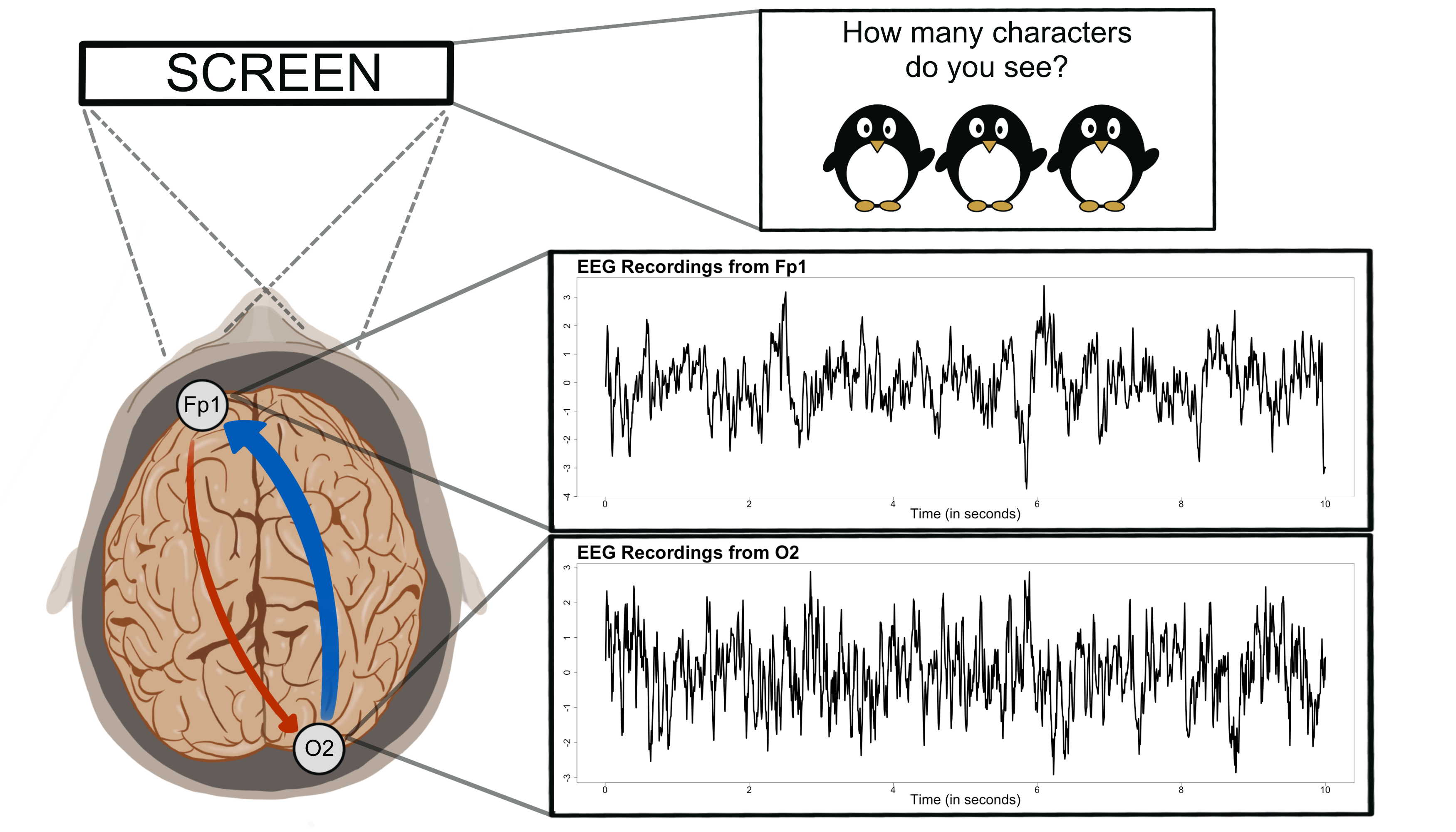
Figure 1: Illustration of a child performing a visual task, collected EEG recordings from some channels, and the hypothesized causal relationship between two brain regions.

Granger causality (GC) is a widely-used causal inference framework to answer such hypotheses. Given two time series $X$ and $Y$, the notion of “$X$ Granger-causes $Y$” implies that the variance of the predictions for $Y$ decreases by considering the past values of another series $X$ together with its own history (Granger, 1963, 1969). Since GC suggests a directional relationship, it offers an elegant foundation for exploring information transfer between signals coming from different brain regions. However, despite its well-built theoretical justifications, several restrictive assumptions (e.g., linearity, additivity and Gaussianity) limits the application of GC in neuroimaging data (Shojaie & Fox, 2022).

Conceptualized by Schreiber (2000), an alternative approach that overcomes these limitations is through the concept of transfer entropy. Transfer entropy (TE) is an information-theoretic measure that quantifies the causal impact of $X$ to $Y$ by calculating the dependence between the current values $Y_{t}$ and the history of the other series, denoted by $\bm{X}_{t-k}$, given its own past $\bm{Y}_{t-\ell}$, for some positive lags $k$ and $\ell$, directly from their conditional distribution. Being equivalent to conditional mutual information (CMI), another dependence measure in information theory (Gray, 2011; Cover & Thomas, 2012), TE shares the same properties as CMI. For example, the interpretation of “zero” TE from $X$ to $Y$ implies conditional independence between $Y_{t}$ and the lagged values $\bm{X}_{t-k}$ given its own lagged values $\bm{Y}_{t-\ell}$. Moreover, TE does not assume any type of relationship between the series or impose any assumption on the distribution of the series. This makes TE a more flexible causal measure than GC that is more suitable in analyzing connectivity in brain data like EEGs.

In EEG analysis, a common objective is to perform inference on the signals that are decomposed/filtered into different frequency bands (e.g., delta (0.5–4 Hz), theta (4–8 Hz), alpha (8–12 Hz), beta (12–30 Hz), and gamma (30–100 Hz); see Ombao et al. (2005); Nunez et al. (2016); Guerrero et al. (2023); Ombao & Pinto (2022)), which have well-known associated cognitive functions (Harmony, 2013; Bjørge & Emaus, 2017). To increase the applicability of TE in neuroscience, its development in the frequency domain becomes crucial. Recent efforts in this interest avoid the use of filtering (“frequency band-specific” analysis) due to its effect of temporal dependence distortion and inability to isolate spectral causality (Barnett & Seth, 2011), thus, implementing their methodologies on the actual spectral representations of the series (“frequency-specific” analysis for individual frequencies). Chen et al. (2019) embedded the phase-space reconstruction method with the two-dimensional Fourier transform, while Tian et al. (2021) derived the theory for using wavelet transformation on the signals before calculating TE. However, these frequency-specific approaches may result in two possible drawbacks: (i) increased family-wise error rate (FWER) in detecting significant spectral causal influence; and (ii) vague practical interpretations.

Given that frequency-specific methods estimate TE for a large number of possible frequencies and for multiple pairs of signal sources, detected significant quantities may be inappropriate even after adjusting for multiple comparisons. Furthermore, if the method employs computational-intensive techniques for testing significance (such as resampling), it is expected to be burdensome as the requirement for the number of replicates per test greatly increases with the number of simultaneous comparisons being tested (to ensure an acceptable precision). In addition, suppose a significant TE is calculated only at a specific frequency in the boundary of two frequency bands, linking these results to established findings may become subjective. Since both issues can potentially minimize the method’s utility for clinicians and neuroscientists, we pursue the use of frequency band-specific filtered signals in developing TE in the frequency domain to attain an easy-to-interpret methodology that allows for controlling the FWER in the brain connectivity analysis.

In this paper, we propose a novel approach to quantify the amount and direction of information transfer between two time series from the frequency-band perspective. Instead of directly calculating TE between two filtered band-specific signals, we develop a new spectral causal measure, which we call the spectral transfer entropy (STE), based on the maximum magnitude of the zero-mean filtered series within overlapping time blocks. This approach, through the lens of extreme value theory, offers a new perspective on capturing causal relationships in a brain network which is, more importantly, robust to the inherent problems of filtering. To minimize the impact of having different marginal characteristics in estimation, we exploit the relationship, proven by Ma & Sun (2011), between copula theory and the information-theoretic measure. More specifically, we develop an estimation procedure via vine copula models after expressing TE in terms of copula densities. By strategically arranging the variables in a D-vine structure (Kurowicka & Cooke, 2005), we demonstrate that one advantage is a simpler re-expression for calculating TE which is capable of capturing the boundary value of zero. Moreover, since generating new observations from an estimated vine copula can be done easily, a convenient resampling method for measuring uncertainty of the estimates, which can readily accommodate correction for multiple comparisons, is implemented.

The remainder of this paper is organized as follows. Section 2 provides a brief review of copula theory, dependence measures in information theory and their established equivalence. In Section 3, we propose our new causal measure in the frequency domain, the STE, and develop a novel estimation method based on vine copula models combined with extreme value theory. To provide evidence on the performance of STE in capturing spectral influence, in Section 4, we use the proposed metric on simulated series. In Section 5, we analyze actual EEG recordings from multiple children with or without attention deficit hyperactivity disorder (ADHD), and report interesting findings and novel results that describes the brain functional connectivity during performance of a visual task. Lastly, some concluding notes and future directions of our work are discussed in Section 6.

2 Quantifying Dependence via Copula Theory and Information Theory

Suppose that $\bm{X}$ is a $d$-dimensional random vector where $F(\bm{x})$ and $f(\bm{x})$ represent its cumulative distibution function (CDF) and probability density function (PDF), respectively. Similar notations are used for other random vectors when the necessity occurs. Here, we present two concepts that characterize dependence between variables, namely, copula theory and information theory. We first describe both concepts based on general random vectors but establish their relationship in the context of time series data afterwards.

2.1 Copula Theory and Vine Copula Models

For any $d$-dimensional CDF $F$ with continuous univariate margins $F_{1},\ldots,F_{d}$, Sklar’s theorem (Sklar, 1959) states that there exists a unique $d$-dimensional copula $C$ (i.e., a joint distribution function with uniform Unif$(0,1)$ margins) such that

$$F(\bm{x})=C\{F_{1}(x_{1}),\ldots,F_{d}(x_{d})\},\leavevmode\nobreak\ \leavevmode\nobreak\ \leavevmode\nobreak\ \bm{x}\in\mathbb{R}^{d}.\vspace{-6.5mm}$$ (1)

An implication of Equation (1) is that, if the CDF $F$ is absolutely continuous, then the joint PDF $f$ can be expressed as

$$f(\bm{x})=c\{F_{1}(x_{1}),\ldots,F_{d}(x_{d})\}\prod^{d}_{i=1}f_{i}(x_{i}),\vspace{-6.5mm}$$ (2)

where $c(\cdot)$ is the corresponding copula density. By Equation (2), the dependence structure of any jointly-distributed continuous random variables can be extracted independently from the marginal distributions. Moreover, given the margins $F_{i}(x_{i}),i=1,\ldots,d$, Aas et al. (2009) showed that any $d$-dimensional copula density can be decomposed as product of bivariate copulas and conditonal bivariate copulas. Although the decomposition is not unique, a graphical method, called regular vines, offers a systematic approach for specifying a valid decomposition (Bedford & Cooke, 2001).

In this work, we focus on a specific vine structure called the D-vine (Kurowicka & Cooke, 2005), because it leads to simplifications for calculating the causal measure of interest, as explained in Section 3.2.2 below. Assuming a D-vine structure, any $d$-dimensional copula density $c(F_{1}(x_{1}),\ldots,F_{d}(x_{d}))$, can be written through conditional bivariate copulas as

$$c(F_{1}(x_{1}),...,F_{d}(x_{d}))=\prod^{d-1}_{j=1}\prod^{d-j}_{i=1}c_{i,i+j|i+1,...,i+j-1}(F(x_{i}|x_{i+1},...,x_{i+j-1}),F(x_{i+j}|x_{i+1},...,x_{i+j-1})).\vspace{-6mm}$$

Under the so-called “simplifying assumption” (Czado & Nagler, 2022), we obtain a valid $d$-dimensional copula model, which spans a rich class of copulas and can be expressed through bivariate copulas only (i.e., without conditioning variables) to be specified by the analyst:

$$c(F_{1}(x_{1}),\ldots,F_{d}(x_{d}))=\prod^{d-1}_{j=1}\prod^{d-j}_{i=1}c_{i,i+j}(F(x_{i}|x_{i+1},\ldots,x_{i+j-1}),F(x_{i+j}|x_{i+1},\ldots,x_{i+j-1})).\vspace{-6mm}$$ (3)

Moreover, by strategically organizing the arrangement of variables in a D-vine of the form (3), the copula density of any subset $\{X_{j_{1}},\ldots,X_{j_{n}}\leavevmode\nobreak\ \mid\leavevmode\nobreak\ j_{1},\ldots,j_{n}\in\{1,\ldots,d\},n\leq d\}$ can be obtained from Equation (3) by extracting the corresponding bivariate copula terms. With this, computations for some information-theoretic measures are simplified, which we exploit in our proposed estimation procedure for the STE.

2.2 Mutual Information and Transfer Entropy

Mutual information (MI) is the key formulation of dependence in information theory (see Cover & Thomas, 2012). More formally, the mutual information between two random vectors $\bm{X}$ and $\bm{Y}$, denoted by $I(\bm{X},\bm{Y})$ is defined as

$$I(\bm{X},\bm{Y})=\iint f(\bm{x},\bm{y})\log\frac{f(\bm{x},\bm{y})}{f(\bm{x})f(\bm{y})}\,\mathop{}\!\mathrm{d}\bm{x}\mathop{}\!\mathrm{d}\bm{y}=D_{KL}(f(\bm{x},\bm{y})\|f(\bm{x})f(\bm{y}))\vspace{-6.5mm}$$ (4)

where $D_{KL}(P_{X}\|P_{Y})$ is the Kullback–Leibler divergence of the distribution $P_{X}$ with respect to $P_{Y}$. In broad terms, MI is a measure of statistical dependence, as it reflects the discrepancy between the true joint probability model and the statistically independent model. Clearly, $I(\bm{X},\bm{Y})=0$ if and only if $\bm{X}$ and $\bm{Y}$ are independent. Since MI does not impose any assumptions on the distribution of the random vectors or the form of relationship between them, it is a very general dependence measure.

Sometimes, the dependence between $\bm{X}$ and $\bm{Y}$ may be driven by another random vector $\bm{W}$. For the simple linear case, this is captured by the partial correlation coefficient (PCC) since it measures the linear relationship between two variables after taking the effects of the conditioning vector out of both variables (see Christensen et al., 2002). However, for nonlinear dependence, the PCC may be inappropriate. Instead, the natural congruent of PCC in the mutual information formulation relies on the conditional mutual information (CMI). By analogy with 4, the conditional mutual information between $\bm{X}$ and $\bm{Y}$ given $\bm{W}$, denoted by $I(\bm{X},\bm{Y}\mid\bm{W})$, is given by

$$I(\bm{X},\bm{Y}\mid\bm{W})=\iiint f(\bm{x},\bm{y},\bm{w})\log\frac{f(\bm{w})f(\bm{x},\bm{y},\bm{w})}{f(\bm{x},\bm{w})f(\bm{y},\bm{w})}\,\mathop{}\!\mathrm{d}\bm{x}\mathop{}\!\mathrm{d}\bm{y}\mathop{}\!\mathrm{d}\bm{w}.\vspace{-6.5mm}$$

As CMI also takes its roots from the Kullback–Leiber divergence, it shares the same properties as MI with application to conditional independence (see Gray, 2011, for a more in-depth discussion). However, one limitation of MI and CMI is that both are symmetric measures, i.e., $I(\bm{X},\bm{Y})=I(\bm{Y},\bm{X})$ and $I(\bm{X},\bm{Y}\mid\bm{W})=I(\bm{Y},\bm{X}\mid\bm{W})$. Hence, they do not indicate any direction of dependence.

To formulate a congruent information-theoretic causal inference metric for time series, Schreiber (2000) developed the concept of transfer entropy. Transfer entropy (TE) from a series $X_{t}$ to another series $Y_{t}$, denoted by $TE(X\rightarrow Y;k,\ell)$, is defined as the CMI between $Y_{t}$ and $\bm{X}_{t-k}$ given $\bm{Y}_{t-\ell}$ where $\bm{X}_{t-k}=(X_{t-1},\ldots,X_{t-k})^{T}$ and $\bm{Y}_{t-\ell}=(Y_{t-1},\dots,Y_{t-\ell})^{T}$. Mathematically,

$$TE(X\rightarrow Y;k,\ell)=I(Y_{t},\bm{X}_{t-k}\mid\bm{Y}_{t-\ell})=\iiint f(y,\bm{y}^{\prime},\bm{x}^{\prime})\log\frac{f(\bm{y}^{\prime})f(y,\bm{y}^{\prime},\bm{x}^{\prime})}{f(y,\bm{y}^{\prime})f(\bm{y}^{\prime},\bm{x}^{\prime})}\,\mathop{}\!\mathrm{d}y\mathop{}\!\mathrm{d}\bm{x}^{\prime}\mathop{}\!\mathrm{d}\bm{y}^{\prime}.\vspace{-6.5mm}$$

In other words, $TE(X\rightarrow Y;k,\ell)$ measures the impact of the lagged values $\bm{X}_{t-k}$ on the series $Y_{t}$ given its own history $\bm{Y}_{t-\ell}$ which is conceptually similar to GC. While TE is based on conditional distributions, GC looks at the improvement in the prediction variance, i.e., stating $X$ “Granger-causes” $Y$ if $\mbox{Var}(\hat{Y}_{t}\mid\bm{Y}_{t-\ell},\bm{X}_{t-k})<\mbox{Var}(\hat{Y}_{t}\mid\bm{Y}_{t-\ell})$, where $\hat{Y}_{t}$ is the optimal predictor of $Y_{t}$ (Ding et al., 2006; Bressler & Seth, 2011). Nonetheless, both frameworks infer the causal influence of one time series to another and Barnett et al. (2009) showed the equivalence of TE and GC under the Gaussianity and linearity assumption.

In this paper, we exploit the link between copula theory and information theory in order to develop an efficient approach for estimating TE in filtered EEG signals. By expressing the joint probability distribution with the corresponding copula density in Equation (2) and some change of variables in the integration, Ma & Sun (2011) showed that MI is related to copula entropy. We use the same technique for TE, viewed as CMI, to obtain the following:

$$\begin{split}TE(X\rightarrow Y;k,\ell)\;&=\int_{[0,1]^{k+\ell+1}}c(u_{y},\bm{u}_{\bm{y}^{\prime}},\bm{u}_{\bm{x}^{\prime}})\log\frac{c(\bm{u}_{\bm{y}^{\prime}})c(u_{y},\bm{u}_{\bm{y}^{\prime}},\bm{u}_{\bm{x}^{\prime}})}{c(u_{y},\bm{u}_{\bm{y}^{\prime}})c(\bm{u}_{\bm{y}^{\prime}},\bm{u}_{\bm{x}^{\prime}})}\,\mathop{}\!\mathrm{d}u_{y}\mathop{}\!\mathrm{d}\bm{u}_{\bm{x}^{\prime}}\mathop{}\!\mathrm{d}\bm{u}_{\bm{y}^{\prime}},\end{split}$$ (5)

where $u_{y}=F(y_{t})$, $\bm{u}_{\bm{y}^{\prime}}=(F(y_{t-1}),\ldots,F(y_{t-\ell}))^{T}$ and $\bm{u}_{\bm{x}^{\prime}}=(F(x_{t-k}),\ldots,F(x_{t-1}))^{T}$ with $F(\cdot)$ as the marginal distribution of the stationary processes $\{X_{t}\}$ and $\{Y_{t}\}$. Hence, we demonstrate a major advantage of our proposed estimation approach: TE estimation requires three but simple independent steps, namely, marginal estimation, copula estimation and integration. For instance, the (nonparametric) empirical distribution function is a usual option to represent the marginal distributions while common techniques for estimating copula densities may be used, e.g., empirical copulas based on ranks or some parametric multivariate copulas. Alternatively, parametric approaches may be used, as in this work. Meanwhile, the last step is straightforward since many numerical methods are available, e.g., Monte Carlo integration, when $k$ and $\ell$ are not too large. Thus, TE, together with its copula representation, offers a general and appropriate framework for causal inference in neural signals with less restrictive assumptions than commonly used.

3 Spectral Transfer Entropy

We now develop a transfer-entropy measure for studying dependence between nodes (channels, voxels or regions) in a brain network. Although classical TE can provide evidence of significant information flow between nodes in a brain network, one limitation is that it does not give any specific information on the oscillatory activities that are involved in this information transfer. Our goal is to develop a metric that captures the magnitude and direction of information flow, say, from a theta-oscillation in one channel to the delta-oscillation in another channel. Our solution is to construct TE in the frequency domain through a new spectral causal measure which we shall call the spectral transfer entropy (STE).

3.1 Definition and General Strategy

Let $\mathcal{X}_{t}$ and $\mathcal{Y}_{t}$ denote the EEG recording at time $t$ of two channels $\mathcal{X}$ and $\mathcal{Y}$, $t=1,\ldots,T$. For $\Omega_{1},\Omega_{2}\in\mathcal{O}=\{\delta,\theta,\alpha,\beta,\gamma\}$, denote by $Z^{\Omega_{1}}_{\mathcal{X},t}$ and $Z^{\Omega_{2}}_{\mathcal{Y},t}$ the latent oscillatory component of $\mathcal{X}_{t}$ and $\mathcal{Y}_{t}$ that are associated with the frequency bands $\Omega_{1}$ and $\Omega_{2}$, respectively. Suppose $\{\mathcal{X}_{t}\}$ and $\{\mathcal{Y}_{t}\}$ are stationary processes that represent mixtures of several oscillatory components. That is, $\mathcal{X}_{t}=g_{\mathcal{X}}(\bm{Z}^{\mathcal{O}}_{\mathcal{X},t})$ and $\mathcal{Y}_{t}=g_{\mathcal{Y}}(\bm{Z}^{\mathcal{O}}_{\mathcal{Y},t})$, where $g_{\mathcal{X}}(\cdot)$ and $g_{\mathcal{Y}}(\cdot)$ are “mixing” functions, $\bm{Z}^{\mathcal{O}}_{\mathcal{X},t}=\big{(}Z^{\delta}_{\mathcal{X},t},Z^{\theta}_{\mathcal{X},t},Z^{\alpha}_{\mathcal{X},t},Z^{\beta}_{\mathcal{X},t},Z^{\gamma}_{\mathcal{X},t}\big{)}^{T}$, and $\bm{Z}^{\mathcal{O}}_{\mathcal{Y},t}=\big{(}Z^{\delta}_{\mathcal{Y},t},Z^{\theta}_{\mathcal{Y},t},Z^{\alpha}_{\mathcal{Y},t},Z^{\beta}_{\mathcal{Y},t},Z^{\gamma}_{\mathcal{Y},t}\big{)}^{T}$. Specifically, $g_{\mathcal{X}}(\cdot)$ and $g_{\mathcal{Y}}(\cdot)$ are functions that combine the contribution of all latent oscillatory components into the observable time series $\{\mathcal{X}_{t}\}$ and $\{\mathcal{Y}_{t}\}$. For instance, a linear mixing function assumes the form $g(\bm{Z})=\bm{a}^{T}\bm{Z}$, where $\bm{a}=\{a_{j}\}^{d}_{j=1}$, $\bm{Z}=\{Z_{j}\}^{d}_{j=1}$ with $a_{j}>0\leavevmode\nobreak\ \forall j$ such that $\sum^{d}_{j=1}a_{j}=1$. Moreover, we do not restrict any interaction between the oscillatory components from each frequency bands, e.g., the theta-oscillations of $\mathcal{X}_{t}$ may have causal influence on the theta-oscillations, as well as the gamma-oscillations, of $\mathcal{Y}_{t}$. Here, the main interest is to derive the causality structure across the different oscillations of $\mathcal{X}_{t}$ and $\mathcal{Y}_{t}$.

In the formulation of STE, since “frequency band-specific” oscillations are known to smoothly fluctuate upwards and downwards, we argue that most of the information about the series are contained among the peaks and among the troughs, or equivalently, among the largest amplitudes (absolute values). Thus, instead of looking at the causality between two oscillatory processes based on every time point, we fix the attention only to the values where the series attain the maximum magnitudes. Define $\mathcal{M}^{\Omega_{1}}_{\mathcal{X},b}=\max\big{(}|Z^{\Omega_{1}}_{\mathcal{X},t}|;t\in\{t_{b}+1,\ldots,t_{b}+m\}\big{)}$ and $\mathcal{M}^{\Omega_{2}}_{\mathcal{Y},b}=\max\big{(}|Z^{\Omega_{2}}_{\mathcal{Y},t}|;t\in\{t_{b}+1,\ldots,t_{b}+m\}\big{)}$ where $t_{b}$ is the time point preceding the $b$-th time block, i.e., $\mathcal{M}^{\Omega_{1}}_{\mathcal{X},b}$ and $\mathcal{M}^{\Omega_{2}}_{\mathcal{Y},b}$ represent the maximum magnitude of the oscillations $Z^{\Omega_{1}}_{\mathcal{X},t}$ and $Z^{\Omega_{2}}_{\mathcal{Y},t}$, respectively, over some time block of length $m$. Explicitly, the objective is to infer the causal impact of $\mathcal{M}^{\Omega_{1}}_{\mathcal{X},b}$ on $\mathcal{M}^{\Omega_{2}}_{\mathcal{Y},b}$ (and vice versa), which is offered by the STE.

We now define the spectral transfer entropy from an oscillatory component $Z^{\Omega_{1}}_{\mathcal{X},t}$ of $\mathcal{X}_{t}$ to the oscillatory component $Z^{\Omega_{2}}_{\mathcal{Y},t}$ of $\mathcal{Y}_{t}$, denoted by $STE_{\Omega_{1},\Omega_{2}}(\mathcal{X}\rightarrow\mathcal{Y};k,\ell)$, as

$$STE_{\Omega_{1},\Omega_{2}}(\mathcal{X}\rightarrow\mathcal{Y};k,\ell)=TE(\mathcal{M}^{\Omega_{1}}_{\mathcal{X}}\rightarrow\mathcal{M}^{\Omega_{2}}_{\mathcal{Y}};k,\ell)=I(\mathcal{M}^{\Omega_{2}}_{\mathcal{Y},b},\bm{\mathcal{M}}^{\Omega_{1}}_{\mathcal{X},b-k}|\bm{\mathcal{M}}^{\Omega_{2}}_{\mathcal{Y},b-\ell}),\vspace{-6.5mm}$$ (6)

where $\bm{\mathcal{M}}^{\Omega_{1}}_{\mathcal{X},b-k}=\big{(}\mathcal{M}^{\Omega_{1}}_{\mathcal{X},b-1},\ldots,\mathcal{M}^{\Omega_{1}}_{\mathcal{X},b-k}\big{)}^{T}$ and $\bm{\mathcal{M}}^{\Omega_{1}}_{\mathcal{Y},b-\ell}=\big{(}\mathcal{M}^{\Omega_{1}}_{\mathcal{Y},b-1},\ldots,\mathcal{M}^{\Omega_{1}}_{\mathcal{Y},b-\ell}\big{)}^{T}$. By its definition, STE enjoys all the nice properties of TE (and CMI). It quantifies the amount of information transferred from a band-specific oscillation of a series to a another oscillation of another series. More importantly, having zero STE implies that one oscillatory component does not have a spectral causal influence to the other. Hence, STE bridges TE to the frequency domain.

However, since $\mathcal{M}^{\Omega_{1}}_{\mathcal{X},b}$ and $\mathcal{M}^{\Omega_{2}}_{\mathcal{Y},b}$ are functions of $Z^{\Omega_{1}}_{\mathcal{X},t}$ and $Z^{\Omega_{2}}_{\mathcal{Y},t}$ which are unobservable latent processes, estimation of STE requires extraction of these oscillatory components from the observed signals. One way to do this is by filtering. The advantage of using the maximum magnitudes over time blocks is that, given the block size $m$ is large enough, it avoids the well-known issues caused by filtering on causal inference in the frequency domain (temporal dependence distortion and false extraction of spectral influence) (see Barnett & Seth, 2011). Precisely, we perform the spectral causal inference based on STE as follows:

1. For $\Omega_{1},\Omega_{2}\in\mathcal{O}$, denote $\{\psi_{j}^{\Omega_{1}}\}$ and $\{\psi_{j}^{\Omega_{2}}\}$ to be the one-sided Butterworth (BW) filter coefficients with gain function concentrated on the bands $\Omega_{1}$ and $\Omega_{2}$, respectively. Define $\mathcal{X}^{\Omega_{1}}_{t}=\sum^{\infty}_{j=-\infty}\psi_{j}^{\Omega_{1}}\mathcal{X}_{t-j}$ and $\mathcal{Y}^{\Omega_{2}}_{t}=\sum^{\infty}_{j=-\infty}\psi_{j}^{\Omega_{2}}\mathcal{Y}_{t-j}$, which represent the extracted band-specific oscillations of $\mathcal{X}_{t}$ and $\mathcal{Y}_{t}$ for the five frequency bands.

2. Let $M^{\Omega_{1}}_{\mathcal{X},b}=\max\big{(}|\mathcal{X}^{\Omega_{1}}_{t}|;t\in\{(b-1)q+1,\ldots,(b-1)q+m\}\big{)}$ and $M^{\Omega_{2}}_{\mathcal{Y},b}=\max\big{(}|\mathcal{Y}^{\Omega_{2}}_{t}|;t\in\{(b-1)q+1,\ldots,(b-1)q+m\}\big{)}$ for $b\in\mathbb{Z}_{+}$ and some step-size $q\leq m$. That is, consider the maximum magnitude (absolute value) of the band-specific series within overlapping time blocks of length $m$ (see Figure 2).

3. Serving as the analogue for $\mathcal{M}^{\Omega_{1}}_{\mathcal{X},b}$ and $\mathcal{M}^{\Omega_{2}}_{\mathcal{Y},b}$, estimate STE based on $M^{\Omega_{1}}_{\mathcal{X},b}$ and $M^{\Omega_{2}}_{\mathcal{Y},b}$ using the proposed estimation discussed below in Section 3.2 and perform significance testing based on the proposed resampling scheme, via the D-vine copula representation, outlined in Section 3.3.

4. Since multiple connections are being tested simultaneously, apply multiple comparison correction (e.g., the Benjamini–Hochberg (BH) method of Benjamini & Hochberg, 1995) on the computed $p$-values to control for the FWER.

Although we do not explore the effect of the choice of the block size $m$ and the step size $q$, we suggest choosing $m$ and $q$ in such a way that the interpretation of information transfer is desirable for the context under study while making sure the marginal fits, based on extreme value theory (see Section 3.2.1), are good enough. For all simulations and analysis throughout the paper, we use $m=s/2$ and $q=m/2$ where $s$ is the sampling rate (in Hz) of the EEG recordings. An implication of $m=s/2$ is that the temporal scale of spectral causal impact captured by the STE metric is “per half a second”. On the other hand, the step-size $q=m/2$ is the conservative option between approximately independent non-overlapping blocks ($q=m$) and highly dependent overlapping blocks ($q=1$).

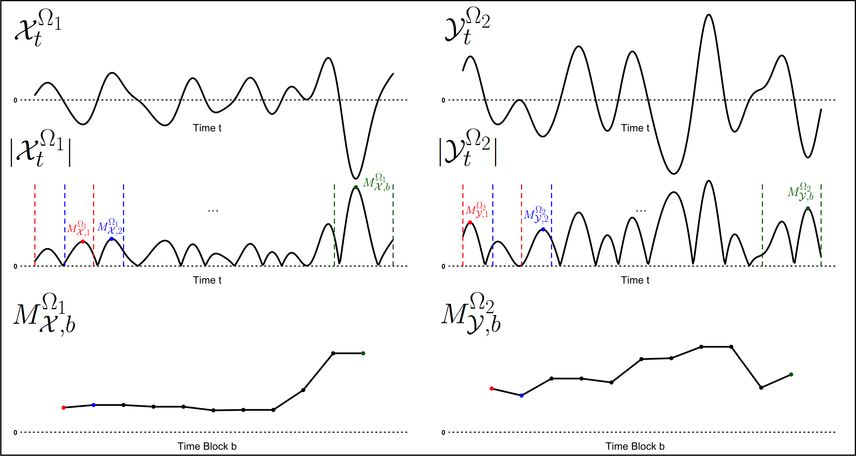
Figure 2: Illustration for the filtered band-specific series $\mathcal{X}^{\Omega_{1}}_{t}$ and $\mathcal{Y}^{\Omega_{2}}_{t}$, their magnitudes $|\mathcal{X}^{\Omega_{1}}_{t}|$ and $|\mathcal{Y}^{\Omega_{2}}_{t}|$, and the computed overlapping block maxima series $M^{\Omega_{1}}_{\mathcal{X},b}$ and $M^{\Omega_{2}}_{\mathcal{Y},b}$.

We stress again that our approach uses the maximum magnitude within overlapping time blocks instead of the actual values of the filtered series across all time points. That is, we extract the information contained in the oscillatory processes through the highest amplitudes before measuring its causal impact onto one another. Hence, the proposed approach is robust to the inherent issues of filtering, in particular, artifacts in connectivity that is induced by the linear filter operator. Moreover, with a small finite number of frequency bands, controlling for FWER becomes feasible unlike for other frequency-specific methods, even when considering multiple channel pairs in the brain network.

3.2 Novel Copula-based Estimation for STE

For the succeeding discussions, we re-label the series of block maxima for given frequency bands as $X_{t}$ and $Y_{t}$ instead of $M^{\Omega_{1}}_{\mathcal{X},b}$ and $M^{\Omega_{2}}_{\mathcal{Y},b}$. This is to avoid using more complex superscripts and subscripts, especially when defining lagged values of the block maxima series in the copula representation. Thus, the shift in notation implies that

$$STE_{\Omega_{1},\Omega_{2}}(\mathcal{X}\rightarrow\mathcal{Y};k,\ell)=TE(\mathcal{M}^{\Omega_{1}}_{\mathcal{X}}\rightarrow\mathcal{M}^{\Omega_{2}}_{\mathcal{Y}};k,\ell)\coloneqq TE(X\rightarrow Y;k,\ell).\vspace{-6.5mm}$$

Now, after extracting the band-specific series and computing the sequence of overlapping block maxima of the series’ magnitudes, the estimation of STE is reduced to two main steps: fitting the marginal distributions for the series of block maxima (Section 3.2.1) and modeling the dependence structure associated with the joint distribution of the block maxima series (Section 3.2.2).

3.2.1 Marginal Distributions based on Extreme Value Theory

Fitting the copula associated with $TE(X\rightarrow Y;k,\ell)$ requires first specifying the marginal distributions of $X_{t}$ and $Y_{t}$. This is an important task because incorrect assumptions on the margins leads to poor fit for the copula model, and thus, results in false characterization of the dependence structure. There are several ways to estimate the margins $F(x_{t})$ and $F(y_{t})$. One convenient option is to use the empirical distribution function since, by the Glivenko–Cantelli Theorem (see e.g., Wasserman (2004)), it converges to the true distribution as the sample size approaches to infinity. However, its validity becomes limited in finite samples, especially when there are too few observations. In such a scenario, an alternative approach is to consider distributions from a parametric family. Since $X_{t}$ and $Y_{t}$ are series of block maxima, an appropriate choice is offered by the generalized extreme value (GEV) distribution. Without loss of generality, suppose $\{W_{j}=|\mathcal{X}^{\Omega}_{t+j-1}|,\Omega\in\mathcal{O},j=1,\ldots,m\}$ is a sequence of independent and identically distributed (IID) random variables and hence, $X_{t}=\max(W_{1},\ldots,W_{m})=\max\big{(}|\mathcal{X}^{\Omega}_{t}|,\ldots,|\mathcal{X}^{\Omega}_{t+m-1}|\big{)}$. By the Extremal Types Theorem (Fisher & Tippett, 1928; Gnedenko, 1943), if there exist sequences of constants $a_{m}>0$ and $b_{m}\in\mathbb{R}$, such that $\lim_{m\rightarrow\infty}\mbox{P}\left[a^{-1}_{m}\{\max(W_{1},\ldots,W_{m})-b_{m}\}\leq x\right]=G(x)$, for some non-degenerate distribution function $G$, then the limit $G$ has the form

$$G(x)=\exp\left[-\Big{\{}1+\xi\Big{(}\frac{x-\mu}{\sigma}\Big{)}\Big{\}}^{-1/\xi}_{+}\right],\vspace{-5mm}$$ (7)

where $a_{+}=\max(0,a)$. Equation (7) defines the GEV distribution with location parameter $\mu$, scale parameter $\sigma$ and shape parameter $\xi$, and this family encompasses the three extreme value limit families: Fréchet ($\xi>0$), reversed Weibull ($\xi<0$) and Gumbel ($\xi=0$); see Coles, 2001. The Fréchet distribution is heavy-tailed, the reversed Weibull distribution has an upper-bounded tail, and the Gumbel distribution is thin-tailed (Bali, 2003). For a concise summary of univariate and multivariate models of extremes, see Davison & Huser (2015).

However, since the sequence $\{\mathcal{X}^{\Omega}_{t}\}$ represents an oscillatory component of the observed EEG recordings, the IID assumption on $W_{j}=|\mathcal{X}^{\Omega}_{t+j-1}|,j=1,\ldots,m$, is not appropriate. In fact, we assume the oscillatory components to be strictly stationary since frequency band-specific series, obtained from applying a linear filter (such as the BW filter) to stationary series, are also stationary (Brockwell & Davis, 2016). When $\{\mathcal{X}^{\Omega}_{t}\}$ is strictly stationary, is it straighforward to show that the absolute value sequence $\big{\{}|\mathcal{X}^{\Omega}_{t}|\big{\}}$ is also strictly stationary, but not IID. Fortunately, the extension of the Extremal Types Theorem to stationary sequences has been long established (Leadbetter, 1983). That is, under mild mixing conditions restricting long-range dependence, the limiting distribution for the renormalized maximum of the stationary sequence is still GEV, although the temporal dependence may modify the location and scale parameters (Davison & Huser, 2015). Hence, assuming GEV margins for each block maxima series $X_{t}$ and $Y_{t}$ suitable a consistent representation of its marginal characteristics for considerably large block length $m$.

3.2.2 Dependence Structure Through the D-vine Construction

After taking into account the marginal characteristics of $X_{t}$ and $Y_{t}$ using the univariate GEV distribution, the next step is to estimate the associated copula structure. While it may be natural to use multivariate max-stable extreme value distributions to model multivariate block maxima (see Coles (2001) for definitions), we purposefully choose not to use such models to describe the dependence structure in our context because of several reasons: (i) it is difficult to model and estimate unstructured max-stable distributions in high dimensions (Davison & Huser, 2015); and (ii) recent research has shown that multivariate max-stable models are often too rigid in their dependence structure leading to poor fit in various applications (Huser & Wadsworth, 2022). In summary, we seek a flexible and fast framework to estimate the STE, and vine copulas meet these requirements. Hence, we assume a vine copula model defined in Section 2.1 and employ the sequential estimation approach proposed by Aas et al. (2009) where the pair copulas that are involved in the decomposition of the $d$-dimensional copula are modelled separately. This allows for a more adaptable specification of the pairwise relationship between the variables as different copula families may be selected for each pair copula.

In addition, by strategically arranging the block maxima series and their respective lagged values as $(Y_{t},Y_{t-1},\ldots,Y_{t-\ell},X_{t-k},\ldots,X_{t-1})^{T}$ (equivalently, as $(u_{y},\bm{u}_{\bm{y}^{\prime}},\bm{u}_{\bm{x}^{\prime}})^{T}$ in (5)) in a D-vine structure, we further simplify the calculation for STE (and TE, in general). More concretely, because the $c(\bm{u}_{\bm{y}^{\prime}})$, $c(u_{y},\bm{u}_{\bm{y}^{\prime}})$, and $c(\bm{u}_{\bm{y}^{\prime}},\bm{u}_{\bm{x}^{\prime}})$ are “subsets” of the full joint copula density, by expressing them into their corresponding D-vine decomposition, some common factors cancel out in the $\log$ component of $TE(X\rightarrow Y;k,\ell)$ (see Figure 3). This simplified form based on the D-vine naturally aligns with the definition of TE, i.e., the remaining pair copulas reflect the relationship between the current value of one series to the past values of another series given its own history. In general, for any $k$ and $\ell$,

$$\log\frac{c(\bm{u}_{\bm{y}^{\prime}})c(u_{y},\bm{u}_{\bm{y}^{\prime}},\bm{u}_{\bm{x}^{\prime}})}{c(u_{y},\bm{u}_{\bm{y}^{\prime}})c(\bm{u}_{\bm{y}^{\prime}},\bm{u}_{\bm{x}^{\prime}})}=\log\prod^{k}_{j=1}c(F(y_{t}|\bm{y}_{t-\ell},\bm{x}_{t-(j+1)}),F(x_{t-j}|\bm{y}_{t-\ell},\bm{x}_{t-(j+1)})),$$ (8)

where $\bm{y}_{t-\ell}=(y_{t-1},\ldots,y_{t-\ell})^{T}$ and $\bm{x}_{t-(j+1)}=(x_{t-(j+1)},x_{t-(j+2)},\ldots,x_{t-k})^{T}$ with $\bm{x}_{t-(k+1)}$ removed from the conditioning set (see Supplementary Material for the case when $k=\ell=2$ and $k=\ell=3$). As a result, the computation for $TE(X\rightarrow Y;k,\ell)$ only requires the remaining conditional bivariate copulas (not the full joint copula density) specified in Equation (8). With this, we estimate $STE_{\Omega_{1},\Omega_{2}}(\mathcal{X}\rightarrow\mathcal{Y};k,\ell)$ as follows:

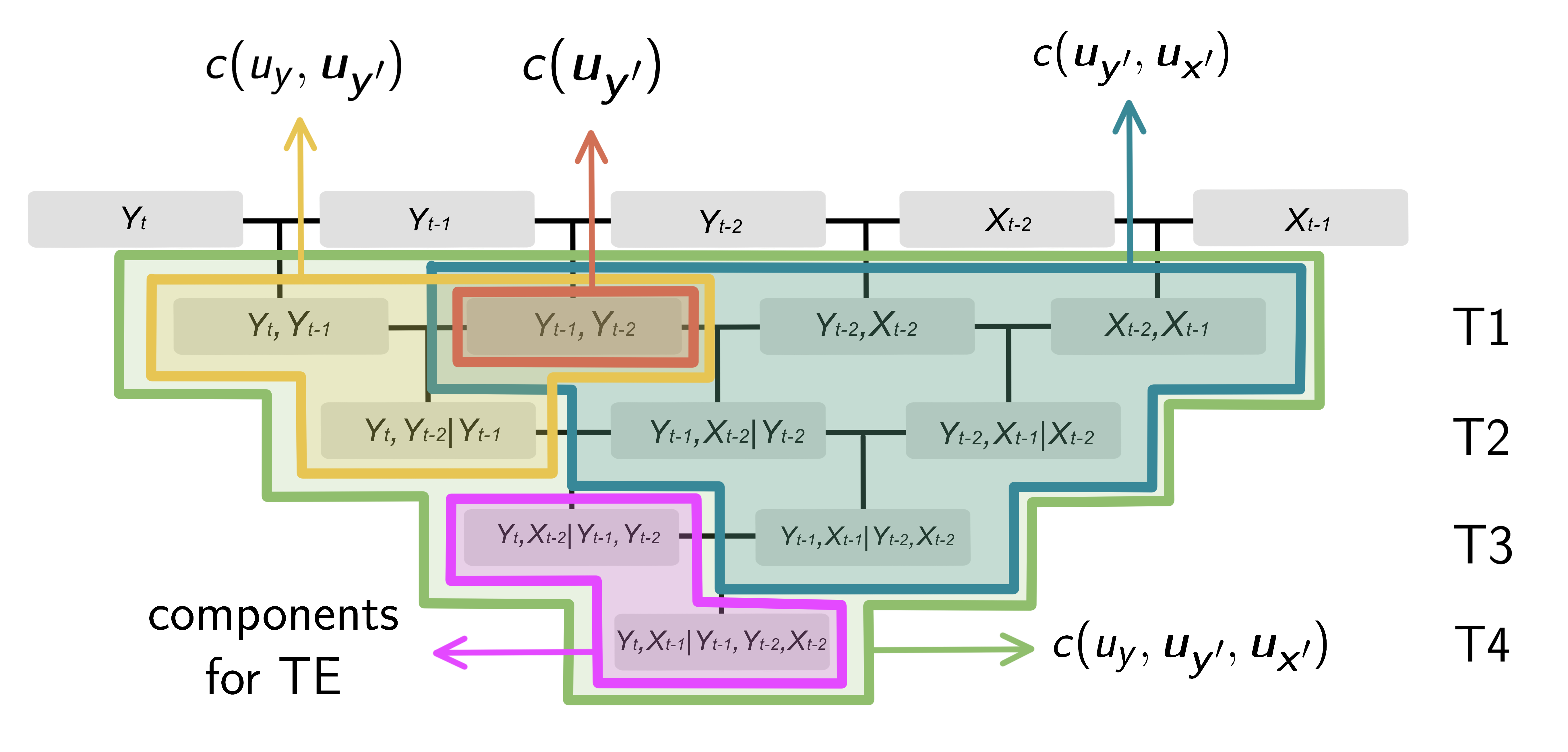
Figure 3: Illustration for calculating $TE(X\rightarrow Y;k=2,\ell=2)$ based on the strategically arranged D-vine copula structure of the series $Y_{t}$ and lagged series ($Y_{t-1},Y_{t-2},X_{t-1},X_{t-2}$).

1. Fit individual GEV distributions for the block maxima series $X_{t}$ and $Y_{t}$ computed from the filtered series, and denote the fitted margins as $\hat{G}(x_{t})$ and $\hat{G}(y_{t})$.

2. For pre-specified $k$ and $\ell$, arrange the variables in the D-vine structure and denote by $(y_{t},y_{t-1},\ldots,y_{t-\ell},x_{t-k},\ldots,x_{t-1},x_{t})^{T}\longrightarrow(u_{y},\bm{u}_{\bm{y}^{\prime}},\bm{u}_{\bm{x}^{\prime}},u_{x})^{T},$ the proposed arrangement of the transformed vector, where $u_{y}=\hat{G}(y_{t})$, $\bm{u}_{\bm{y}^{\prime}}=(\hat{G}(y_{t-1}),\ldots,\hat{G}(y_{t-\ell}))^{T}$, $\bm{u}_{\bm{x}^{\prime}}=(\hat{G}(x_{t-k}),\ldots,\hat{G}(x_{t-1}))^{T}$, and $u_{x}=\hat{G}(x_{t})$.

3. Fit a vine copula model to $(u_{y},\bm{u}_{\bm{y}^{\prime}},\bm{u}_{\bm{x}^{\prime}},u_{x})^{T}$ using the sequential estimation procedure developed by Aas et al. (2009). That is, for each pair copula in the decomposition, we select the “best” bivariate copula family among a chosen collection of copula models, based on some information criterion (e.g., modified Bayesian information criterion for vines (mBICv) (Nagler et al., 2019)), and estimate the parameters of the chosen families. Choices for the bivariate copula selection may include the independence copula, elliptical copulas (e.g., Gaussian and Student’s $t$), Archimedean copulas (Clayton, Frank, and Joe), and extreme value copulas (e.g., Gumbel), or transformations thereof.

4. Using the estimated vine copula, from Equation (8) and Monte Carlo integration, the estimator for $STE_{\Omega_{1},\Omega_{2}}(\mathcal{X}\rightarrow\mathcal{Y};k,\ell)$ is given by
   $\widehat{STE}_{\Omega_{1},\Omega_{2}}(\mathcal{X}\rightarrow\mathcal{Y};k,\ell)\leavevmode\nobreak\ \leavevmode\nobreak\ =\leavevmode\nobreak\ \leavevmode\nobreak\ \widehat{TE}(X\rightarrow Y;k,\ell)$

   $$\leavevmode\nobreak\ \leavevmode\nobreak\ \leavevmode\nobreak\ \leavevmode\nobreak\ \leavevmode\nobreak\ \leavevmode\nobreak\ \leavevmode\nobreak\ \leavevmode\nobreak\ \leavevmode\nobreak\ \leavevmode\nobreak\ \leavevmode\nobreak\ \leavevmode\nobreak\ \leavevmode\nobreak\ \leavevmode\nobreak\ \leavevmode\nobreak\ \leavevmode\nobreak\ \leavevmode\nobreak\ \leavevmode\nobreak\ \leavevmode\nobreak\ \leavevmode\nobreak\ \leavevmode\nobreak\ \leavevmode\nobreak\ \leavevmode\nobreak\ \leavevmode\nobreak\ \leavevmode\nobreak\ \leavevmode\nobreak\ =\frac{\sum^{T}_{t=p+1}\log\prod^{k}_{j=1}\hat{c}(F(y_{t}|\bm{y}_{t-\ell},\bm{x}_{t-(j+1)}),F(x_{t-j}|\bm{y}_{t-\ell},\bm{x}_{t-(j+1)}))}{T-p},\vspace{-3.5mm}$$

   where $p=\max\{k,\ell\}$ and the $\hat{c}(\cdot,\cdot)$s are the estimated pair copula densities in Step (3).

An advantage of our approach is its ability to provide estimates at the boundary point zero. Existing estimation procedures for TE requires “shuffling” to adjust the estimates from the bias due to finite sample effects (Marschinski & Kantz, 2002). However, our method is robust to this problem. Whenever independent copulas are selected for the remaining conditional bivariate copula in Equation (8), the estimated TE attains an exact value of zero, thus removing the necessity for bias adjustment. Another advantage is that the estimate for the other causal direction, denoted by $\widehat{STE}_{\Omega_{2},\Omega_{1}}(\mathcal{Y}\rightarrow\mathcal{X};\ell,k)=\widehat{TE}(Y\rightarrow X;\ell,k)$, can be directly obtained from the same estimated vine copula model for $(u_{y},\bm{u}_{\bm{y}^{\prime}},\bm{u}_{\bm{x}^{\prime}},u_{x})^{T}$. Hence, the new estimation scheme that we introduce provides a simple and efficient way for calculating STE in both causal directions based on a single fitted model, which reduces model selection bias.

3.3 A Resampling Method for Testing Significance of Spectral Transfer Entropy

Suppose we wish to test the following null hypothesis $H_{0}$,

$$\begin{split}H_{0}:\;&STE_{\Omega_{1},\Omega_{2}}(\mathcal{X}\rightarrow\mathcal{Y};k,\ell)=TE(X\rightarrow Y;k,\ell)=0\\ \text{vs.\leavevmode\nobreak\ \leavevmode\nobreak\ }H_{1}:\;&STE_{\Omega_{1},\Omega_{2}}(\mathcal{X}\rightarrow\mathcal{Y};k,\ell)=TE(X\rightarrow Y;k,\ell)>0.\end{split}\vspace{-3.5mm}$$

Under the null hypothesis, $TE(X\rightarrow Y;k,\ell)=0$ implies that the corresponding pair copulas $c(F(y_{t}|\bm{y}_{t-\ell},\bm{x}_{t-(j+1)}),F(x_{t-j}|\bm{y}_{t-\ell},\bm{x}_{t-(j+1)}))$, for $j=1,\ldots,k$, are all equal to the independence copula. This enables simulating observations under $H_{0}$ from the estimated vine copula $\hat{C}(u_{y},\bm{u}_{\bm{y}^{\prime}},\bm{u}_{\bm{x}^{\prime}},u_{x})$ based on the original data.

Denote the vine copula model under the null hypothesis as $C^{(0)}(u_{y},\bm{u}_{\bm{y}^{\prime}},\bm{u}_{\bm{x}^{\prime}},u_{x})$. The pair copulas involved in $C^{(0)}(\cdot)$ are the same bivariate copulas as those from the estimated $\hat{C}(\cdot)$ except for the components that are specifically associated with $TE(X\rightarrow Y;k,\ell)$ which we replace by the independence copula (see Figure 4). Thus, new observations generated from $C^{(0)}(\cdot)$ preserve the dependence structure within each block maxima series $X$ and $Y$, but eliminate the information transfer from the past values $\bm{X}_{t-k}$ to $Y_{t}$. Repeatedly estimating TE from these generated observations then provides an empirical distribution of the estimator under the null hypothesis of no information transfer. Hence, we perform testing for significance of $TE(X\rightarrow Y;k,\ell)$ based on the outline below:

1. Generate new observations from the null vine copula model $C^{(0)}(\cdot)$ of the same size as the original data.

2. Estimate $TE(X\rightarrow Y;k,\ell)$ from the new observations using the proposed copula-based estimation procedure and denote the estimates by $\widehat{TE}^{(b)}(X\rightarrow Y;k,\ell)$.

3. Compute the $p$-value for testing the significance of the estimate $\widehat{TE}(X\rightarrow Y;k,\ell)$ as the relative frequency of the event $\{\widehat{TE}^{(b)}(X\rightarrow Y;k,\ell)\geq\widehat{TE}(X\rightarrow Y;k,\ell)\}$ among all resamples considered ($b=1,\ldots,B$).

4. Given a specified level of significance $\alpha\in(0,1)$, reject the null hypothesis if the $p$-value is less than $\alpha$. Otherwise, do not reject $H_{0}$.

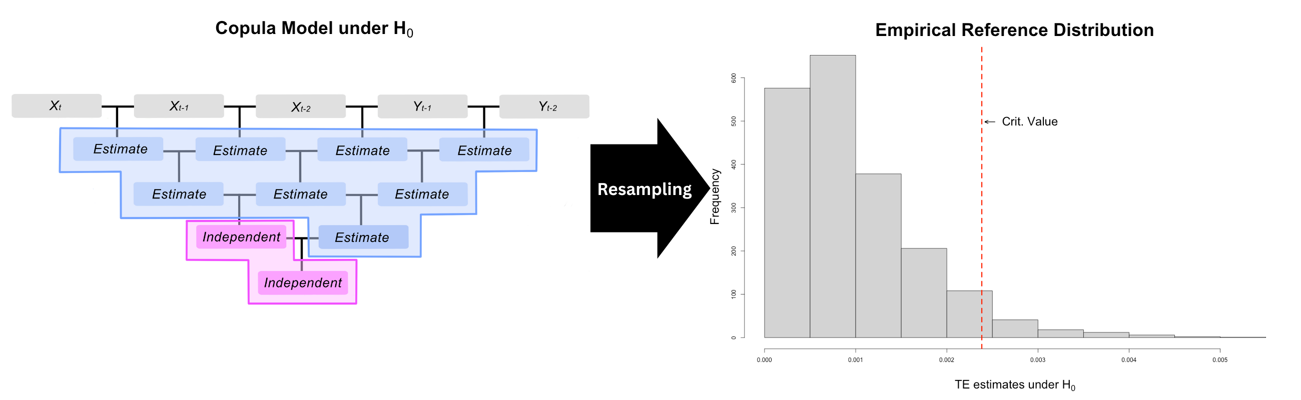
Figure 4: The copula model under the null hypothesis and the generated empirical reference distribution for hypothesis testing.

Another benefit offered by our procedure is the convenience in measuring uncertainties of the estimates. Since new observations can be easily generated from the null vine copula model, computing for significance levels (i.e., the associated $p$-values) using standard resampling methods is relatively fast even with large number of replicates (to achieve an acceptable precision for multiple comparison adjustments). Moreover, simultaneously testing for both directions ($TE(X\rightarrow Y)$ and $TE(Y\rightarrow X)$) may be implemented from the same null copula model which greatly lessens the computational costs and model selection bias. Such feature is desirable in studying brain connectivity, especially when considering multiple pairs of nodes in a brain network while, at the same time, taking into account several oscillatory components.

4 Numerical Experiments

In this section, we explore the ability of our proposed causal metric for capturing information transfer in the frequency domain through realistic EEG simulations driven by the characterization that these signals are a function of oscillations at various frequency bands. Particularly, we provide evidence on the utility of STE in detecting significant and non-significant flow of information across different frequency oscillations, which may come in both linear and nonlinear forms. In addition, we illustrate its robustness to the issues imposed by linear filtering, in comparison to the standard Wald test for Granger causality (Lütkepohl & Reimers, 1992), that is based on a fitted vector autoregressive (VAR) model.

We generated several pairs of unit-variance latent processes (at sampling rate $s=100$ Hz) based on their respective autoregressive (AR) representations, following Ombao & Pinto (2022) and Granados-Garcia et al. (2022), to mimic the five standard frequency bands: delta (0.5–4 Hz), theta (4–8 Hz), alpha (8–12 Hz), beta (12–30 Hz), and gamma (30–45 Hz). Denote $\{Z^{\Omega}_{\mathcal{X},t},Z^{\Omega}_{\mathcal{Y},t}\}$ to be the pair of latent processes coming from the same frequency band $\Omega$ where $\Omega\in\{\delta,\theta,\alpha,\beta,\gamma\}$. We induce the causal relationship between $Z^{\Omega}_{\mathcal{X},t}$ and $Z^{\Omega}_{\mathcal{Y},t}$ in three possible scenarios: (i) there is no information transfer in any direction, (ii) there is a “one-sided” information transfer, e.g., only $Z^{\Omega}_{\mathcal{X},t}\rightarrow Z^{\Omega}_{\mathcal{Y},t}$ is significant but not the other direction, and (iii) there is a “two-sided” information transfer, i.e., both $Z^{\Omega}_{\mathcal{X},t}\rightarrow Z^{\Omega}_{\mathcal{Y},t}$ and $Z^{\Omega}_{\mathcal{Y},t}\rightarrow Z^{\Omega}_{\mathcal{X},t}$ are significant. For $\Omega\in\{\beta,\gamma\}$, we simulate $Z^{\Omega}_{\mathcal{X},t}$ and $Z^{\Omega}_{\mathcal{Y},t}$ from independent AR($2$) processes which results in the first case of no information transfer. On the other hand, a VAR($2$) model is used to simulate the “one-sided” information transfer between $Z^{\Omega}_{\mathcal{X},t}$ and $Z^{\Omega}_{\mathcal{Y},t}$ where $\Omega\in\{\delta,\theta\}$. Lastly, for the “two-sided” information transfer case, we use a vector autoregressive moving average (VARMA) model of order $(2,2)$ to simulate the alpha-band pair $\{Z^{\alpha}_{\mathcal{X},t},Z^{\alpha}_{\mathcal{Y},t}\}$. Details on the models used for simulation are reported in the Supplementary Material.

In addition, we simulate the theta-gamma ($\theta$–$\gamma$) coupling phenomenon by modulating the amplitude of the gamma latent process with the magnitude of the theta latent process, i.e., $Z^{\gamma}_{\mathcal{Y}^{*},t}=\mbox{sgn}(Z^{\gamma}_{\mathcal{Y},t})\times|Z^{\theta}_{\mathcal{X},t}|$ where $\mbox{sgn}(x)=x/|x|$ for $x\neq 0$ ($0$ otherwise); see Figure 5. Then, we define two series $\mathcal{X}_{t}$ and $\mathcal{Y}_{t}$ as a linear mixing function of the latent processes, that is, $\mathcal{X}_{t}=g_{\mathcal{X}}(Z^{\delta}_{\mathcal{X},t},Z^{\theta}_{\mathcal{X},t},Z^{\alpha}_{\mathcal{X},t},Z^{\beta}_{\mathcal{X},t},Z^{\gamma}_{\mathcal{X},t-s},W_{\mathcal{X},t})$ and $\mathcal{Y}_{t}=g_{\mathcal{Y}}(Z^{\delta}_{\mathcal{Y},t},Z^{\theta}_{\mathcal{Y},t},Z^{\alpha}_{\mathcal{Y},t},Z^{\beta}_{\mathcal{Y},t},Z^{\gamma}_{\mathcal{Y}^{*},t},W_{\mathcal{Y},t})$, where $g_{\mathcal{X}}(\cdot)$ and $g_{\mathcal{Y}}(\cdot)$ are linear functions with coefficients summing to one, and $W_{\mathcal{X},t},W_{\mathcal{Y},t}\overset{\mathrm{iid}}{\sim}N(0,1)$. Specifically, all band-specific unit-variance latent oscillations are weighted equally in the linear mixture, and the coefficients are chosen such that the signal-to-noise ratio is around 95%. This ensures that the BW filter can adequately extract the oscillations and the detected causal relationships are solely because of the proposed method — not artifacts of poor filtering. Meanwhile, the ability of the choice of filter to successfully extract the oscillatory components is outside the scope of this work. With this, we explicitly simulate five directions of information transfer to be significant, namely $Z^{\delta}_{\mathcal{Y},t}\rightarrow Z^{\delta}_{\mathcal{X},t}$, $Z^{\theta}_{\mathcal{X},t}\rightarrow Z^{\theta}_{\mathcal{Y},t}$, $Z^{\theta}_{\mathcal{X},t}\rightarrow Z^{\gamma}_{\mathcal{Y},t}$, $Z^{\alpha}_{\mathcal{X},t}\rightarrow Z^{\alpha}_{\mathcal{Y},t}$, and $Z^{\alpha}_{\mathcal{Y},t}\rightarrow Z^{\alpha}_{\mathcal{X},t}$, while the rest are non-significant. We emphasize that all simulated causal influence in the same frequency band, e.g., from delta-to-delta oscillations, are linear by the nature of VAR and VARMA models. Meanwhile, the cross-frequency ($\theta$–$\gamma$) coupling exhibit nonlinear information transfer since the absolute value of the theta-oscillations modulates the magnitude of the gamma-oscillations. The novelty of STE is that it captures all (i.e., both linear and nonlinear) types of causal relationships.

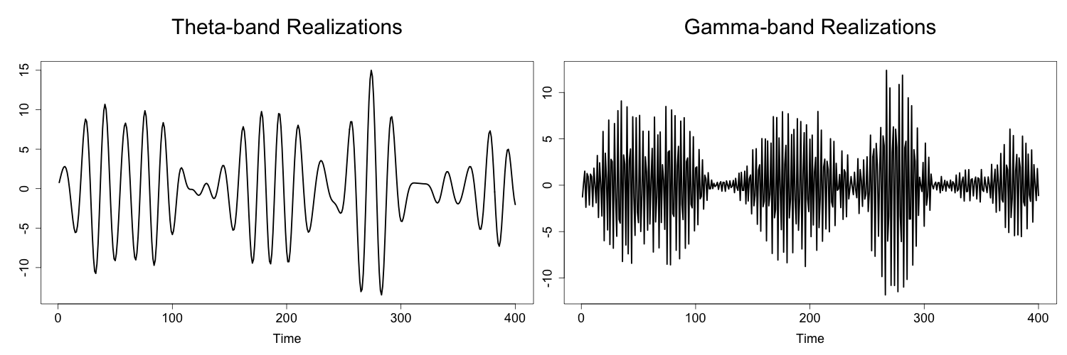
Figure 5: Simulated theta-gamma coupling phenomenon.

Figure 6 shows the empirical distribution of the STE estimates over three different time series lengths based on $1000$ simulation replicates. Our proposed spectral causal metric successfully estimates non-zero values for cases that have significant information transfers while estimating near-zero STE values for independent cases. Furthermore, there is a visible reduction in the uncertainty of the estimates given more observations, which roughly decreases like the square root of the time series length, as typically expected. This hints at the consistency of our estimation procedure.

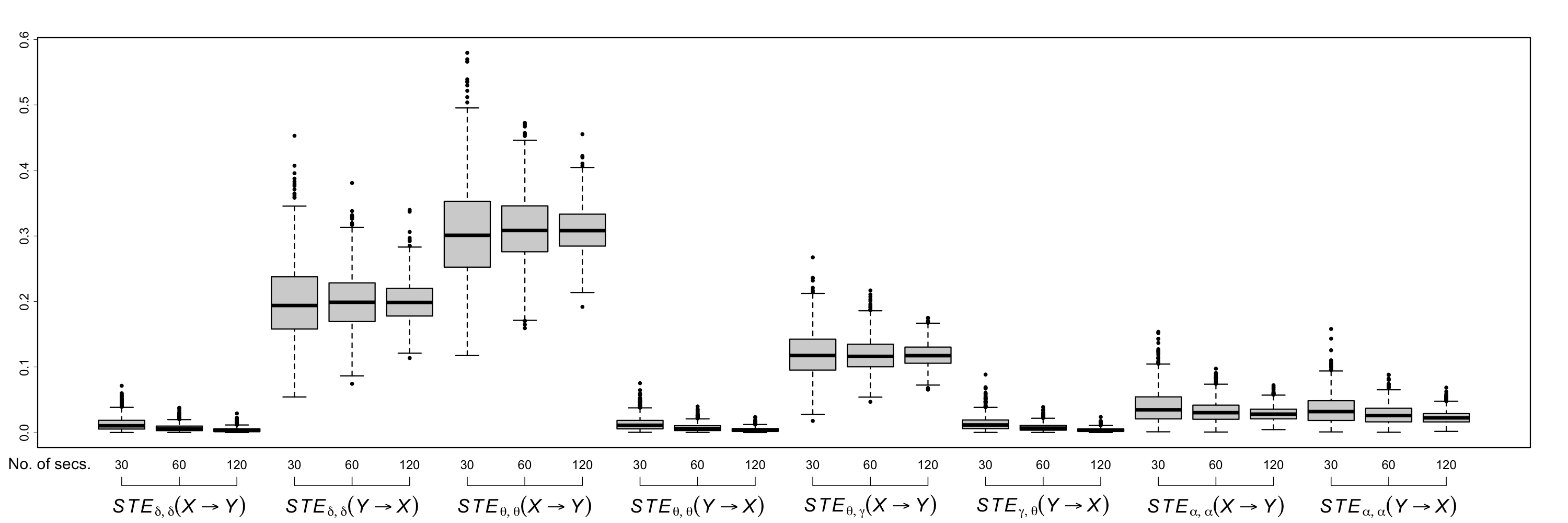
Figure 6: Estimated STE between the filtered frequency band-specific series $\mathcal{X}^{\Omega_{1}}_{t}$ and $\mathcal{Y}^{\Omega_{2}}_{t}$ for selected frequency bands $\Omega_{1}$ and $\Omega_{2}$ based from $1000$ simulation replicates.

Table 1: Proportion of significant “frequency band-specific” causal link based on the standard Wald test for GC and the proposed STE metric from $1000$ simulation replicates (considering level of significance $\alpha=0.05$).

$\mathbf{\mathcal{X}\rightarrow\mathcal{Y}}$	No. of secs.	STE	WGC	$\mathbf{\mathcal{Y}\rightarrow\mathcal{X}}$	No. of secs.	STE	WGC
	30	0.047	1.000		30	1.000	1.000
${\delta\rightarrow\delta}$	60	0.053	1.000	${\delta\rightarrow\delta}\leavevmode\nobreak\ \leavevmode\nobreak\ (*)$	60	1.000	1.000
	120	0.070	1.000		120	1.000	1.000
	30	1.000	1.000		30	0.040	1.000
${\theta\rightarrow\theta}\leavevmode\nobreak\ \leavevmode\nobreak\ (*)$	60	1.000	1.000	${\theta\rightarrow\theta}$	60	0.050	1.000
	120	1.000	1.000		120	0.078	1.000
	30	0.996	0.000		30	0.044	0.000
${\theta\rightarrow\gamma}\leavevmode\nobreak\ \leavevmode\nobreak\ (*)$	60	1.000	0.000	${\gamma\rightarrow\theta}$	60	0.054	0.000
	120	1.000	0.000		120	0.062	0.000
	30	0.454	0.983		30	0.390	0.996
${\alpha\rightarrow\alpha}\leavevmode\nobreak\ \leavevmode\nobreak\ (*)$	60	0.780	1.000	${\alpha\rightarrow\alpha}\leavevmode\nobreak\ \leavevmode\nobreak\ (*)$	60	0.685	1.000
	120	0.984	1.000		120	0.935	1.000
	30	0.056	0.457		30	0.068	0.454
${\beta\rightarrow\beta}$	60	0.041	0.664	${\beta\rightarrow\beta}$	60	0.071	0.641
	120	0.050	0.886		120	0.054	0.878
	30	0.071	0.221		30	0.065	0.325
${\gamma\rightarrow\gamma}$	60	0.047	0.190	${\gamma\rightarrow\gamma}$	60	0.045	0.272
	120	0.046	0.198		120	0.056	0.323

The simulated significant “frequency band-specific” causal links are marked with $(*)$.

Moreover, we compare our methodology with the standard Wald test for Granger causality (WGC) based on an estimated VAR($2$) model fitted to the filtered series. Table 1 shows the proportion of detected significant causal links based on the STE and WGC for some selected pairs of frequency bands based on $1000$ simulation replicates (considering a $0.05$ level of significance). For the cases where there is no information transfer between oscillatory components, our STE metric achieves correct sizes, i.e., the proportions of false detection are close to the specified nominal level. When the information transfer occurs only in one direction (e.g., $Z^{\theta}_{\mathcal{X},t}\rightarrow Z^{\theta}_{\mathcal{Y},t}$), the STE captures this link with high power, even for the cross-coupling modulation. However, in the case where the spectral link is two-sided (e.g., $Z^{\alpha}_{\mathcal{X},t}\leftrightarrow Z^{\alpha}_{\mathcal{Y},t}$), our approach has relatively low power but improves drastically with more observations. Nonetheless, the results show the robustness of our method to the problems induced by linear filtering as the STE calculated from filtered series still yields high power while remaining correctly sized.

On the other hand, the WGC test clearly suffers from the inherent problems of filtering. Due to the temporal dependence distortion, the WGC test rejects the null hypothesis of no information transfer with high probability regardless if the causal link is either significant or non-significant. This makes the WGC test incorrectly sized which limits its utility in real data applications. Furthermore, since the WGC test assumes linearity in the effect of one series to the other, it is unable to detect non-linear causal relationships such as the cross-coupling modulation. Thus, our STE metric offers a more appropriate tool for studying brain functional connectivity in the frequency domain.

5 EEG Analysis: Brain Connectivity During Visual Task

The goal of this paper is to characterize the brain functional connectivity, during cognition, of children diagnosed with attention deficit hyperactivity disorder (ADHD), in comparison to children without any registered psychiatric disorder (healthy control). Specifically, we want to find causal relationships between brain regions of subjects with ADHD that significantly differ from a healthy subject’s connectivity. Another objective is to establish the connection of such relationships to specific frequency bands that have well-known associated cognitive functions. This enables for a better understanding of the neurological dysfunctions associated with ADHD. For these purposes, existing methods are inadequate because of either too simplistic or too restrictive assumptions. Moreover, these approaches construct the causal structure in the “frequency-specific” paradigm which, most of the time, is hard to interpret and has high risk of inflated FWER. Thus, we develop a new spectral causal framework, our STE approach, in order to address these scientific questions.

Here, we investigate brain connectivity by analyzing EEG recordings of two groups of children (the ADHD group and healthy control group) during performance of a visual task. The data, collected by Motie Nasrabadi et al. (2020), contains samples of EEGs at 128Hz, from 19 channels of 51 children with ADHD and 53 healthy subjects. To remove unwanted artifacts and increase the quality of the recordings, pre-processing was conducted via the PREP pipeline of Bigdely-Shamlo et al. (2015). Then, the pre-processed EEGs were standardized to a unified scale (zero-mean unit variance series). The visual-cognitive experiment was to count the number of characters in a flashed image (recall Figure 1). Hence, to “represent” brain regions that are highly likely to be engaged during the cognitive task, we selected six EEG channels, namely, Fp1 (left pre-frontal), Fp2 (right pre-frontal), T7 (left temporal), T8 (right temporal), O1 (left occipital) and O2 (right occipital) (see Figure 7b). Given that the frontal region is linked with concentration, focus and problem solving, the temporal region with speech and memory, and the occipital region with visual processing (Bjørge & Emaus, 2017), the interest now is to identify (in both the ADHD and control groups) which cross-channel information transfer is significant and at which frequency bands it occurs.

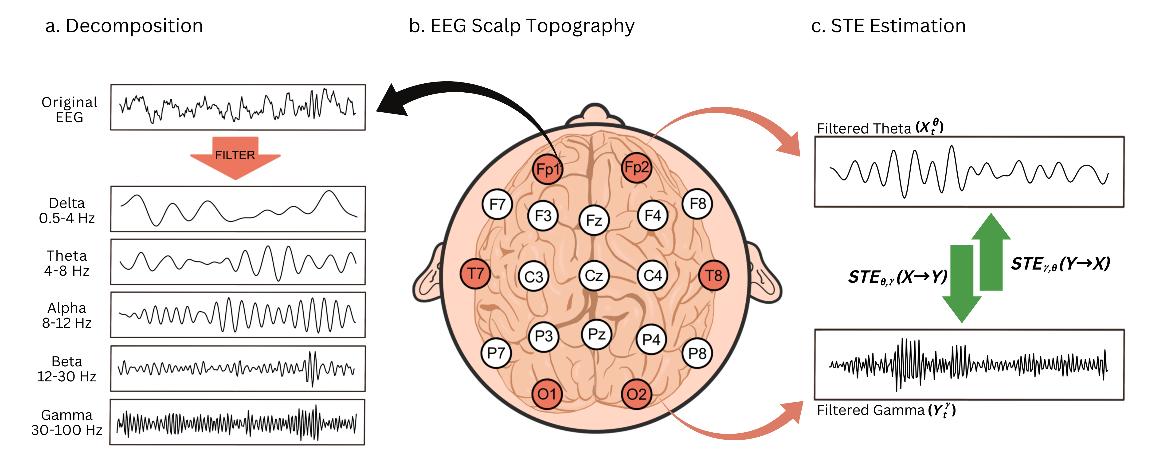
Figure 7: Building blocks of STE. (a) Application of bandpass filter on original EEG series to obtain frequency band-specific filtered series. (b) Standard 10–20 EEG scalp topography where the highlighted channels are included in the analysis. (c) Illustration for STE estimation between two filtered series.

During the experiment, the succeeding images are flashed right after the subject answers how many characters are in the shown picture. This ensures that the EEG recordings reflects the continuous thinking process associated to the visual task without any interruptions. Arguably, this continuity justifies that the series we use for estimating the STE are approximately stationary. To obtain the filtered frequency band-specific series per channel, $4^{th}$ order Butterworth band-pass filters are applied to the standardized and pre-processed EEG series (see Figure 7a). Then, we calculate the STE for each possible pair of the selected channels and for each pair of possible frequency bands (see Figure 7c). Tests for significance of the calculated STEs are conducted based on $B=500$ resamples. Since there are $\binom{6}{2}=15$ channel pairs, $5\times 5=25$ frequency band pairs, and $2$ causal directions, a total of $750$ individual significance tests for each subject are implemented and their corresponding BH-adjusted $p$-values are used to describe the brain connectivity of the two groups.

Table 2: Summary of significant “frequency band”-specific causal links based on the proposed STE metric detected from at least $30\%$ of subjects in the group after multiple comparison adjustments.

Causal Link	ADHD	Control	Causal Link	ADHD	Control
$Fp1(\theta)\rightarrow Fp2(\delta)$	$\usym{1F5F8}$	$\usym{1F5F8}$	$Fp1(\theta)\rightarrow O2(\delta)$	$\usym{1F5F8}$	$\usym{1F5F8}$
$Fp1(\delta)\rightarrow O1(\delta)$	$\usym{1F5F8}$	$\usym{1F5F8}$	$Fp1(\theta)\rightarrow T7(\delta)$		$\usym{1F5F8}$
$Fp1(\theta)\rightarrow O1(\delta)$	$\usym{1F5F8}$	$\usym{1F5F8}$	$Fp1(\theta)\rightarrow T8(\delta)$		$\usym{1F5F8}$
$Fp2(\delta)\rightarrow Fp1(\delta)$	$\usym{1F5F8}$		$Fp2(\delta)\rightarrow O2(\delta)$	$\usym{1F5F8}$	$\usym{1F5F8}$
$Fp2(\theta)\rightarrow Fp1(\delta)$	$\usym{1F5F8}$	$\usym{1F5F8}$	$Fp2(\theta)\rightarrow O2(\delta)$	$\usym{1F5F8}$	$\usym{1F5F8}$
$Fp2(\delta)\rightarrow O1(\delta)$	$\usym{1F5F8}$	$\usym{1F5F8}$	$Fp2(\theta)\rightarrow T7(\delta)$	$\usym{1F5F8}$
$Fp2(\theta)\rightarrow O1(\delta)$	$\usym{1F5F8}$	$\usym{1F5F8}$	$Fp2(\theta)\rightarrow T8(\delta)$	$\usym{1F5F8}$
$T7(\delta)\rightarrow O1(\delta)$		$\usym{1F5F8}$	$T8(\theta)\rightarrow O2(\delta)$	$\usym{1F5F8}$
$T8(\delta)\rightarrow O1(\delta)$		$\usym{1F5F8}$	$T8(\theta)\rightarrow T7(\delta)$		$\usym{1F5F8}$
$T8(\delta)\rightarrow O2(\delta)$		$\usym{1F5F8}$

Table 2 summarizes all the spectral causal links detected in at least $30\%$ of the subjects in each group by our STE metric. An interesting insight is that the prominent connections occur in the delta and theta frequency bands. Activity in the delta oscillations is related to the phenomenon of requiring attention to internal processing, i.e., selectively suppressing unnecessary or irrelevant neural activity to accomplish a mental task (Fernández et al., 1995; Harmony et al., 1996). Since the subjects are performing the repetitive task of counting characters, this is necessary to maintaining focus. On the other hand, the theta frequency band is associated with sustained attention (Clayton et al., 2015; Behzadnia et al., 2017). Moreover, for each subject, the estimated spectra from all channel recordings are majorly concentrated in the low (delta and theta) frequency bands. Thus, the detected connections that occur in these two frequency bands are highly plausible.

Additionally, we visualize the estimated brain connectivity network for the ADHD and healthy control groups in Figure 8. An arrow indicates that at least $30\%$ of the subjects in the group has significant spectral information flow between the linked channels. Similar causal links between the two pre-frontal channels and the two occipital channels are observed for both the ADHD and the control groups. The derived causal relationships suggest that information transfer happens from the problem solving channels (Fp1 and Fp2) to the visual processing channels (O1 and O2), which we refer to as the direct link between the pre-frontal and occipital regions. During the process of counting images, this phenomenon describes the brain activity when an individual intentionally stares at an object. We expect these causal links to appear in both groups as all subjects performed the same visual task.

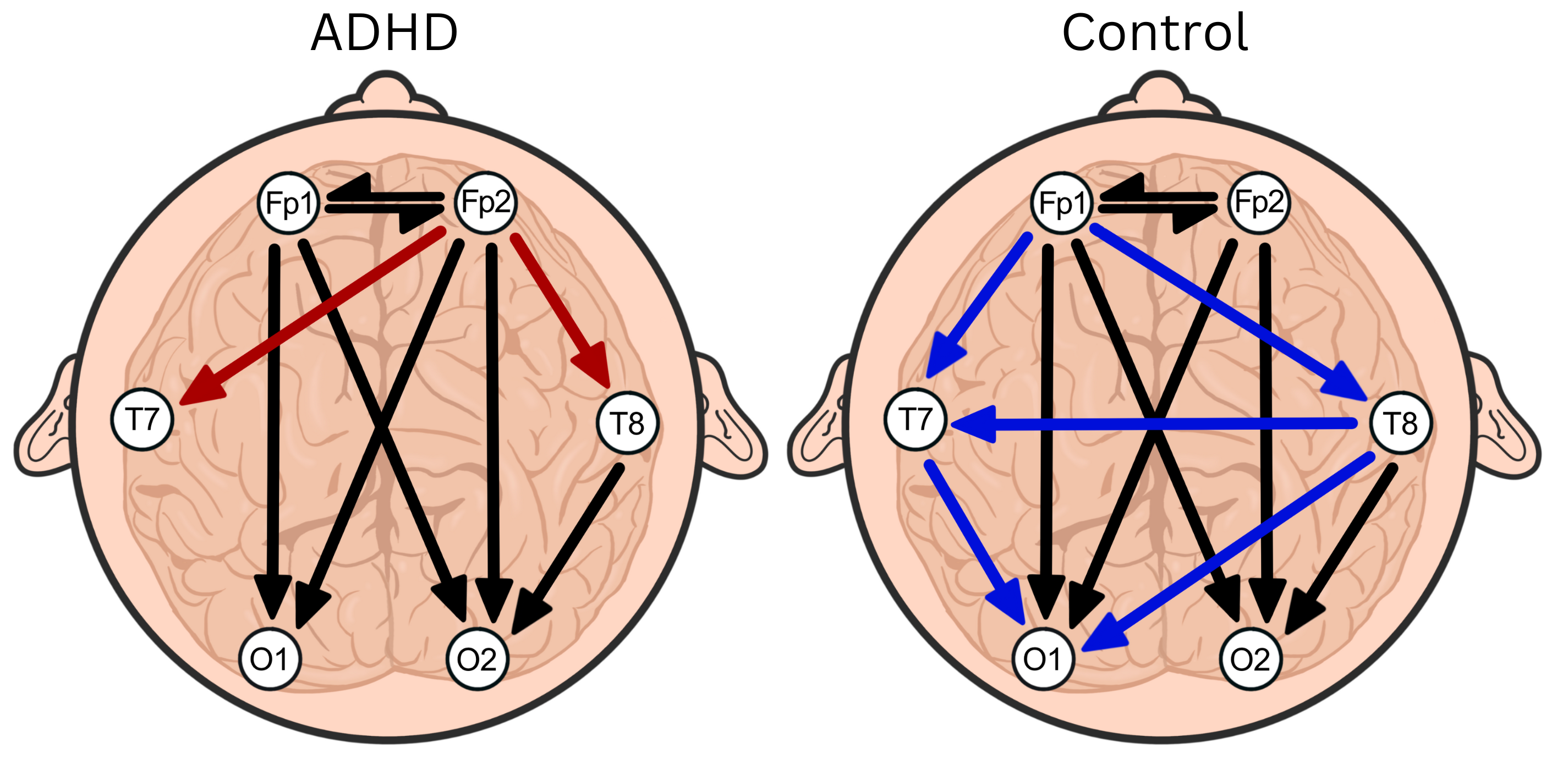
Figure 8: Derived brain connectivity network associated with the visual task for the two groups based on the STE with multiple comparison adjustments. Significant spectral information flow are represented by arrows (black — detected in both groups; red — detected only in the ADHD group; blue — detected only in the control group).

On the other hand, the main difference between the ADHD and control groups is the spectral causal link from the temporal channels (T7 and T8) to the occipital channels (O1 and O2). Consider the information flow from the pre-frontal channels to the occipital channels that passes through the temporal channels. We associate these spectral causal relationships as the indirect link between the pre-frontal and occipital regions. For the ADHD group, we see only a single indirect link. By contrast, there are multiple indirect links for the control group, especially with the significant spectral information transfer between the two temporal channels. We speculate that the information transferred from the indirect links, which occur more prominently in the control group, complements the spectral information flow from the direct links which translates to the efficiency of the thinking process of healthy subjects in performing the visual task.

6 Conclusion

During performance of a specific cognitive task, interactions between different brain regions occur in the form of information transfer. When an individual suffers from a neurodevelopmental disorder, such as ADHD, information flow between some brain regions may be altered (e.g., removed or weakened) compared to a healthy individual, reflecting cognitive dysfunctions. In EEG analysis, this phenomenon can be visualized through the magnitude of cross-channel information flow. Thus, it is important to have a quantitative metric that adequately captures the magnitude and direction of this information transfer between the nodes of an individual’s brain network.

Transfer entropy (TE), an information-theoretic measure, offers a general framework for quantifying the flow of information between two channels. As several brain functions are attributed to specific groups of frequency oscillations (frequency bands), application of TE in the frequency domain becomes more desirable. Thus, we have proposed a new causal metric called spectral transfer entropy (STE) by calculating TE on overlapping block maxima series computed from the magnitude of filtered “frequency band-specific” signals.

The advantage of our proposed STE is that it provides the magnitude of information transfer from a specific oscillatory component of a series to another oscillatory component of another series. It yields higher utility to clinicians since its interpretations are directly linked to standard frequency bands, unlike other works on TE in the frequency domain (which are “frequency-specific” for individual frequencies, rather than “frequency band-specific”). Furthermore, our proposed methodology easily allows for adjustment for multiple comparisons which are often not addressed in its frequency-specific counterparts. With this, the risk of detecting spurious information transfer is no longer an issue since controlling for the family-wise error rate (FWER) is straightforward.

In addition, we propose a novel estimation method for TE/STE that combines vine copulas and extreme value theory. Given that TE/STE can be expressed through the conditional mutual information (CMI), calculations for TE/STE are simplified by considering an appropriate D-vine structure for the full joint copula density. This results in a simpler and more efficient way of estimating TE/STE based on a single fitted model that can be used for both causal directions. Another advantage of our approach is that it is able to obtain an exact “zero” TE, which removes the necessity of adjusting the estimates for bias. Moreover, measuring uncertainty of the estimates based on a standard resampling scheme is fast because generating new observations from an estimated vine copula is straightforward. Numerical experiments illustrate that our inference approach attains correct sizes and high power, providing evidence on the robustness of STE to the issues imposed by filtering.

Our novel STE measure provides interesting findings in the analysis of EEG data linked to a visual task. Prominent connections occur in the delta and theta bands which are associated with maintaining focus and sustained attention. Direct and indirect links from the pre-frontal to the occipital region have been established, in relation to the thinking process involved in counting images. Fewer indirect links (through the temporal regions) differentiate the ADHD group from the control group, hence explaining the efficiency of healthy subjects in performing the experiment.

Even though the STE measure is developed for oscillatory processes, it could also be used for any other time series, although it may then be more appropriate to call it a “tail” transfer entropy (TTE) metric, since it measures the amount of information transferred from the tail of the distribution of one time series to another series’ tail. In this work, we express the tails of two series based on block maxima. For applications that require looking at block minima or a combination of block maxima and block minima, e.g., in modeling extremal causal relationships in stock prices, this can be straightforwardly done in the TTE framework as well.

Lastly, since the STE measure uses the maximum magnitude over time blocks to capture information transfer between oscillatory processes, a natural extension is to consider using high threshold exceedances instead. That is, utilize the data from all time points where the value of the series exceeds some high threshold. However, an issue with this approach is defining the temporal scale of information transfer because exceedances do not happen on equally-spaced time intervals. This makes establishing “how much of the past causes the present” unclear. Nonetheless, combining extreme value theory with modeling causal relationships is a new and novel approach, which may address existing issues of standard methods in understanding brain connectivity.

Supplementary Material for
“Measuring Information Transfer Between Nodes in a Brain Network through Spectral Transfer Entropy”

Paolo Victor Redondo, Raphaël Huser and Hernando Ombao
King Abdullah University of Science and Technology

S1 Illustration for the Simplification of Transfer Entropy under the Vine Copula Representation

An advantage of the proposed vine copula representation for transfer entropy (TE) is that it further simplify the calculation for TE (and for our proposed spectral transfer entropy (STE) metric). To illustrate this, we show the simplification for the case when $k=\ell=2$ and $k=\ell=3$. Suppose $\{X_{t}\}$ and $\{Y_{t}\}$ are strictly stationary processes and denote their respective marginal distributions as $F(x_{t})$ and $F(y_{t})$. Let $u_{y}=F(y_{t})$, $\bm{u}_{\bm{y}^{\prime}}=(F(y_{t-1}),\ldots,F(y_{t-\ell}))^{T}$ and $\bm{u}_{\bm{x}^{\prime}}=(F(x_{t-k}),\ldots,F(x_{t-1}))^{T}$.

For the case when $k=\ell=2$, the copula densities $c(u_{y},\bm{u}_{\bm{y}^{\prime}},\bm{u}_{\bm{x}^{\prime}})$, $c(\bm{u}_{\bm{y}^{\prime}})$, $c(u_{y},\bm{u}_{\bm{y}^{\prime}})$ and $c(\bm{u}_{\bm{y}^{\prime}},\bm{u}_{\bm{x}^{\prime}})$, based on the D-vine structure, can be represented as follows:

$$\begin{split}c(u_{y},\bm{u}_{\bm{y}^{\prime}},\bm{u}_{\bm{x}^{\prime}})=\;&c(F(y_{t}),F(y_{t-1}))c(F(y_{t-1}),F(y_{t-2}))c(F(y_{t-2}),F(x_{t-2}))c(F(x_{t-2}),F(x_{t-1}))\\ &\times c(F(y_{t}|y_{t-1}),F(y_{t-2}|y_{t-1}))c(F(y_{t-1}|y_{t-2}),F(x_{t-2}|y_{t-2}))\\ &\times c(F(y_{t-2}|x_{t-2}),F(x_{t-1}|x_{t-2}))c(F(y_{t}|y_{t-1},y_{t-2}),F(x_{t-2}|y_{t-1},y_{t-2}))\\ &\times c(F(y_{t-1}|y_{t-2},x_{t-2}),F(x_{t-1}|y_{t-2},x_{t-2}))\\ &\times c(F(y_{t}|y_{t-1},y_{t-2},x_{t-2}),F(x_{t-1}|y_{t-1},y_{t-2},x_{t-2}))\\ c(\bm{u}_{\bm{y}^{\prime}})=\;&c(F(y_{t-1}),F(y_{t-2}))\\ \end{split}$$

$$\begin{split}c(u_{y},\bm{u}_{\bm{y}^{\prime}})=\;&c(F(y_{t}),F(y_{t-1}))c(F(y_{t-1}),F(y_{t-2}))c(F(y_{t}|y_{t-1}),F(y_{t-2}|y_{t-1}))\\ c(\bm{u}_{\bm{y}^{\prime}},\bm{u}_{\bm{x}^{\prime}})=\;&c(F(y_{t-1}),F(y_{t-2}))c(F(y_{t-2}),F(x_{t-2}))c(F(x_{t-2}),F(x_{t-1}))\\ &\times c(F(y_{t-1}|y_{t-2}),F(x_{t-2}|y_{t-2}))c(F(y_{t-2}|x_{t-2}),F(x_{t-1}|x_{t-2}))\\ &\times c(F(y_{t-1}|y_{t-2},x_{t-2}),F(x_{t-1}|y_{t-2},x_{t-2}))\end{split}$$

Thus, after cancellation of common factors, we get

$$\begin{split}\log\frac{c(\bm{u}_{\bm{y}^{\prime}})c(u_{y},\bm{u}_{\bm{y}^{\prime}},\bm{u}_{\bm{x}^{\prime}})}{c(u_{y},\bm{u}_{\bm{y}^{\prime}})c(\bm{u}_{\bm{y}^{\prime}},\bm{u}_{\bm{x}^{\prime}})}=\log\{\;&c(F(y_{t}|y_{t-1},y_{t-2}),F(x_{t-2}|y_{t-1},y_{t-2}))\\ &\times c(F(y_{t}|y_{t-1},y_{t-2},x_{t-2}),F(x_{t-1}|y_{t-1},y_{t-2},x_{t-2}))\leavevmode\nobreak\ \}\end{split}$$

On the other hand, when $k=\ell=3$, the copula densities can be represented as follows:

$$\begin{split}c(u_{y},\bm{u}_{\bm{y}^{\prime}},\bm{u}_{\bm{x}^{\prime}})=\;&c(F(y_{t}),F(y_{t-1}))c(F(y_{t-1}),F(y_{t-2}))c(F(y_{t-2}),F(y_{t-3}))c(F(y_{t-3}),F(x_{t-3}))\\ &\times c(F(x_{t-3}),F(x_{t-2}))c(F(x_{t-2}),F(x_{t-1}))c(F(y_{t}|y_{t-1}),F(y_{t-2}|y_{t-1}))\\ &\times c(F(y_{t-1}|y_{t-2}),F(y_{t-3}|y_{t-2}))c(F(y_{t-2}|y_{t-3}),F(x_{t-3}|y_{t-3}))\\ &\times c(F(y_{t-3}|x_{t-3}),F(x_{t-2}|x_{t-3}))c(F(x_{t-3}|x_{t-2}),F(x_{t-1}|x_{t-2}))\\ &\times c(F(y_{t}|y_{t-1},y_{t-2}),F(y_{t-3}|y_{t-1},y_{t-2}))c(F(y_{t-1}|y_{t-2},y_{t-3}),F(x_{t-3}|y_{t-2},y_{t-3}))\\ &\times c(F(y_{t-2}|y_{t-3},x_{t-3}),F(x_{t-2}|y_{t-3},x_{t-3}))c(F(y_{t-3}|x_{t-3},x_{t-2}),F(x_{t-1}|x_{t-3},x_{t-2}))\\ &\times c(F(y_{t}|y_{t-1},y_{t-2},y_{t-3}),F(x_{t-3}|y_{t-1},y_{t-2},y_{t-3}))\\ &\times c(F(y_{t-1}|y_{t-2},y_{t-3},x_{t-3}),F(x_{t-2}|y_{t-2},y_{t-3},x_{t-3}))\\ &\times c(F(y_{t-2}|y_{t-3},x_{t-3},x_{t-2}),F(x_{t-1}|y_{t-3},x_{t-3},x_{t-2}))\\ &\times c(F(y_{t}|y_{t-1},y_{t-2},y_{t-3},x_{t-3}),F(x_{t-2}|y_{t-1},y_{t-2},y_{t-3},x_{t-3}))\\ &\times c(F(y_{t-1}|y_{t-2},y_{t-3},x_{t-3},x_{t-2}),F(x_{t-1}|y_{t-2},y_{t-3},x_{t-3},x_{t-2}))\\ &\times c(F(y_{t}|y_{t-1},y_{t-2},y_{t-3},x_{t-3},x_{t-2}),F(x_{t-1}|y_{t-1},y_{t-2},y_{t-3},x_{t-3},x_{t-2}))\end{split}$$

$$\begin{split}c(\bm{u}_{\bm{y}^{\prime}})=\;&c(F(y_{t-1}),F(y_{t-2}))c(F(y_{t-2}),F(y_{t-3}))c(F(y_{t-1}|y_{t-2}),F(y_{t-3}|y_{t-2}))\\ c(u_{y},\bm{u}_{\bm{y}^{\prime}})=\;&c(F(y_{t}),F(y_{t-1}))c(F(y_{t-1}),F(y_{t-2}))c(F(y_{t-2}),F(y_{t-3}))\\ &\times c(F(y_{t}|y_{t-1}),F(y_{t-2}|y_{t-1}))c(F(y_{t-1}|y_{t-2}),F(y_{t-3}|y_{t-2}))\\ &\times c(F(y_{t}|y_{t-1},y_{t-2}),F(y_{t-3}|y_{t-1},y_{t-2}))\\ c(\bm{u}_{\bm{y}^{\prime}},\bm{u}_{\bm{x}^{\prime}})=\;&c(F(y_{t-1}),F(y_{t-2}))c(F(y_{t-2}),F(y_{t-3}))c(F(y_{t-3}),F(x_{t-3}))c(F(x_{t-3}),F(x_{t-2}))\\ &\times c(F(x_{t-2}),F(x_{t-1}))c(F(y_{t-1}|y_{t-2}),F(y_{t-3}|y_{t-2}))c(F(y_{t-2}|y_{t-3}),F(x_{t-3}|y_{t-3}))\\ &\times c(F(y_{t-3}|x_{t-3}),F(x_{t-2}|x_{t-3}))c(F(x_{t-3}|x_{t-2}),F(x_{t-1}|x_{t-2}))\\ &\times c(F(y_{t-1}|y_{t-2},y_{t-3}),F(x_{t-3}|y_{t-2},y_{t-3}))c(F(y_{t-2}|y_{t-3},x_{t-3}),F(x_{t-2}|y_{t-3},x_{t-3}))\\ &\times c(F(y_{t-3}|x_{t-3},x_{t-2}),F(x_{t-1}|x_{t-3},x_{t-2}))\\ &\times c(F(y_{t-1}|y_{t-2},y_{t-3},x_{t-3}),F(x_{t-2}|y_{t-2},y_{t-3},x_{t-3}))\\ &\times c(F(y_{t-2}|y_{t-3},x_{t-3},x_{t-2}),F(x_{t-1}|y_{t-3},x_{t-3},x_{t-2}))\\ &\times c(F(y_{t-1}|y_{t-2},y_{t-3},x_{t-3},x_{t-2}),F(x_{t-1}|y_{t-2},y_{t-3},x_{t-3},x_{t-2}))\\ \end{split}$$

Hence, the cancellation of common factors gives

$$\begin{split}\log\frac{c(\bm{u}_{\bm{y}^{\prime}})c(u_{y},\bm{u}_{\bm{y}^{\prime}},\bm{u}_{\bm{x}^{\prime}})}{c(u_{y},\bm{u}_{\bm{y}^{\prime}})c(\bm{u}_{\bm{y}^{\prime}},\bm{u}_{\bm{x}^{\prime}})}=\;&\log\{c(F(y_{t}|y_{t-1},y_{t-2},y_{t-3}),F(x_{t-3}|y_{t-1},y_{t-2},y_{t-3}))\\ &\times c(F(y_{t}|y_{t-1},y_{t-2},y_{t-3},x_{t-3}),F(x_{t-2}|y_{t-1},y_{t-2},y_{t-3},x_{t-3}))\\ &\times c(F(y_{t}|y_{t-1},y_{t-2},y_{t-3},x_{t-3},x_{t-2}),F(x_{t-1}|y_{t-1},y_{t-2},y_{t-3},x_{t-3},x_{t-2}))\leavevmode\nobreak\ \}\end{split}$$

S2 Model Specifics for the Numerical Experiments

A second-order autoregressive (AR($2$)) process $Z_{t}$ admits the representation $Z_{t}-\phi_{1}Z_{t-1}-\phi_{2}Z_{t-2}=W_{t}$, where $W_{t}$ is a zero-mean white noise process with $\mbox{Var}(W_{t})=\sigma^{2}_{W}$. Following S_shumway2017time, the spectrum of $Z_{t}$ at a specific frequencey $\omega$, is given by

$$f_{Z}(\omega)=\frac{\sigma^{2}_{W}}{|1-\phi_{1}\exp^{-2\pi i\omega}-\phi_{2}\exp^{-4\pi i\omega}|^{2}}.$$

where $i=\sqrt{-1}$. S_granados2022brain and S_ombao2022spectral showed that there is a one-to-one relationship between the parameter pairs $(\phi_{1},\phi_{2})$ and $(\psi,L)$ where $\psi\in(0,0.5)$ denotes the peak of the spectrum of $Z_{t}$ and $L>0$ controls the spread of the spectrum around the peak $\psi$. Thus, one can simulate from specific frequency bands by considering the appropriate peak parameter $\psi$ and spread parameter $L$. Figure S1 illustrates some simulated frequency bands and their respective spectrum via the AR($2$) model.

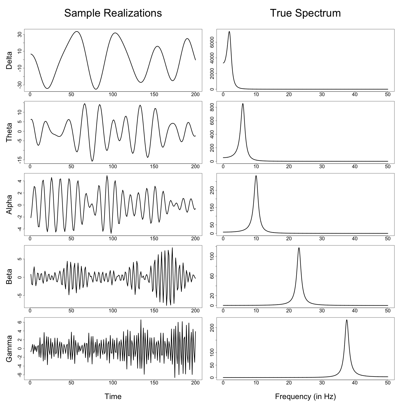
Figure S1: Sample realizations of the generated frequency band-specific latent processes and their corresponding true spectrum.

Table S1: Summary of parameters used to simulate frequency band-specific oscillations (at sampling rate $s=100$ Hz) via the AR($2$) representation based on $(\psi,L)$.

Frequency Band	Time Series Notation	Peak Parameter $\psi$	Spread Parameter $L$
Delta	$Z^{\delta}_{t}$	$2/s$	0.03
Theta	$Z^{\theta}_{t}$	$6/s$	0.03
Alpha	$Z^{\alpha}_{t}$	$10/s$	0.03
Beta	$Z^{\beta}_{t}$	$22.5/s$	0.05
Gamma	$Z^{\gamma}_{t}$	$37.5/s$	0.05

Table S1 summarizes the choice of $(\psi,L)$ to simulate each frequency band-specific oscillations. For $\Omega\in\{\delta,\theta,\alpha,\beta,\gamma\}$, denote the specified peak and spread parameter as $(\psi^{\Omega},L^{\Omega})$ and their corresponding AR(2) coefficients as $(\phi^{\Omega}_{1},\phi^{\Omega}_{2})$. Now, denote by $\{Z^{\Omega}_{\mathcal{X},t},Z^{\Omega}_{\mathcal{Y},t}\}$ the pair of latent processes coming from the same frequency band $\Omega$. There are three possible causal relationship between $Z^{\Omega}_{\mathcal{X},t}$ and $Z^{\Omega}_{\mathcal{Y},t}$: (i) there is no information transfer in any direction, (ii) there is a “one-sided” information transfer, and (iii) there is a “two-sided” information transfer.

For the first case, we consider two independent AR(2) processes, i.e.,

$$\begin{pmatrix}Z^{\Omega}_{\mathcal{X},t}\\ Z^{\Omega}_{\mathcal{Y},t}\end{pmatrix}=\begin{pmatrix}\phi^{\Omega}_{1}&0\\ 0&\phi^{\Omega}_{1}\end{pmatrix}\begin{pmatrix}Z^{\Omega}_{\mathcal{X},t-1}\\ Z^{\Omega}_{\mathcal{Y},t-1}\end{pmatrix}+\begin{pmatrix}\phi^{\Omega}_{2}&0\\ 0&\phi^{\Omega}_{2}\end{pmatrix}\begin{pmatrix}Z^{\Omega}_{\mathcal{X},t-2}\\ Z^{\Omega}_{\mathcal{Y},t-2}\end{pmatrix}+\begin{pmatrix}W_{\mathcal{X},t}\\ W_{\mathcal{Y},t}\end{pmatrix},$$

where $W_{\mathcal{X},t}$ and $W_{\mathcal{Y},t}$ are independent zero-mean white noise (WN) processes with common variance $\sigma_{W}^{2}$. Here, each series is affected only by its own past values, hence there is no information transfer between the two series. To simulate the “one-sided” information transfer, we consider a second-order vector autoregressive (VAR($2$)) process with the following parameterization:

$$\begin{pmatrix}Z^{\Omega}_{\mathcal{X},t}\\ Z^{\Omega}_{\mathcal{Y},t}\end{pmatrix}=\begin{pmatrix}\phi^{\Omega}_{1}&\phi^{\Omega}_{1}\\ 0&\phi^{\Omega}_{1}\end{pmatrix}\begin{pmatrix}Z^{\Omega}_{\mathcal{X},t-1}\\ Z^{\Omega}_{\mathcal{Y},t-1}\end{pmatrix}+\begin{pmatrix}\phi^{\Omega}_{2}&\phi^{\Omega}_{2}\\ 0&\phi^{\Omega}_{2}\end{pmatrix}\begin{pmatrix}Z^{\Omega}_{\mathcal{X},t-2}\\ Z^{\Omega}_{\mathcal{Y},t-2}\end{pmatrix}+\begin{pmatrix}W_{\mathcal{X},t}\\ W_{\mathcal{Y},t}\end{pmatrix},$$

where $W_{\mathcal{X},t},W_{\mathcal{Y},t}\overset{\mathrm{indep.}}{\sim}WN(0,\sigma_{W}^{2})$. Clearly, $Z^{\Omega}_{\mathcal{Y},t}$ is affected only by its own past values while $Z^{\Omega}_{\mathcal{X},t}$ is affected by the past values of both series. Thus, there is information transfer from $Z^{\Omega}_{\mathcal{Y},t}$ to $Z^{\Omega}_{\mathcal{X},t}$, but not from $Z^{\Omega}_{\mathcal{X},t}$ to $Z^{\Omega}_{\mathcal{Y},t}$, which we refer to as the “one-sided” information transfer. Meanwhile, the “two-sided” information transfer between the two series is simulated using the vector autoregressive moving average (VARMA) process with the following specifications:

$$\begin{split}\begin{pmatrix}Z^{\Omega}_{\mathcal{X},t}\\ Z^{\Omega}_{\mathcal{Y},t}\end{pmatrix}=\;&\begin{pmatrix}\phi^{\Omega}_{1}&0\\ \phi^{\Omega}_{1}&0\end{pmatrix}\begin{pmatrix}Z^{\Omega}_{\mathcal{X},t-1}\\ Z^{\Omega}_{\mathcal{Y},t-1}\end{pmatrix}+\begin{pmatrix}\phi^{\Omega}_{2}&0\\ \phi^{\Omega}_{2}&0\end{pmatrix}\begin{pmatrix}Z^{\Omega}_{\mathcal{X},t-2}\\ Z^{\Omega}_{\mathcal{Y},t-2}\end{pmatrix}\\ &+\begin{pmatrix}W_{\mathcal{X},t}\\ W_{\mathcal{Y},t}\end{pmatrix}+\begin{pmatrix}\phi^{\Omega}_{1}&\phi^{\Omega}_{1}\\ 0&\phi^{\Omega}_{1}\end{pmatrix}\begin{pmatrix}W_{\mathcal{X},t-1}\\ W_{\mathcal{Y},t-1}\end{pmatrix}+\begin{pmatrix}\phi^{\Omega}_{2}&\phi^{\Omega}_{2}\\ 0&\phi^{\Omega}_{2}\end{pmatrix}\begin{pmatrix}W_{\mathcal{X},t-2}\\ W_{\mathcal{Y},t-2}\end{pmatrix}\end{split}$$

where $W_{\mathcal{X},t},W_{\mathcal{Y},t}\overset{\mathrm{indep.}}{\sim}WN(0,\sigma_{W}^{2})$. It is straightforward to show that for the specified VARMA process with Gaussian random error components, the distribution of $Z^{\Omega}_{\mathcal{X},t}$ and $Z^{\Omega}_{\mathcal{Y},t}$ both depends on $(Z^{\Omega}_{\mathcal{X},t-1},Z^{\Omega}_{\mathcal{X},t-2},Z^{\Omega}_{\mathcal{Y},t-1},Z^{\Omega}_{\mathcal{Y},t-2})$. Thus, $Z^{\Omega}_{\mathcal{X},t}$ and $Z^{\Omega}_{\mathcal{Y},t}$ depend on their own past values and the past values of the other series, hence the “two-sided” information transfer. Lastly, the frequency band-specific oscillations from all considered cases are standardized to become unit-variance processes before generating the mixture that represents the simulated EEG recordings.

agsm 9_suppref

References

- (1)
- Aas et al. (2009) Aas, K., Czado, C., Frigessi, A. & Bakken, H. (2009), ‘Pair-copula constructions of multiple dependence’, Insurance: Mathematics and Economics 44(2), 182–198.
- Bali (2003) Bali, T. G. (2003), ‘The generalized extreme value distribution’, Economics Letters 79(3), 423–427.
- Barnett et al. (2009) Barnett, L., Barrett, A. B. & Seth, A. K. (2009), ‘Granger causality and transfer entropy are equivalent for Gaussian variables’, Physical Review Letters 103(23), 238701.
- Barnett & Seth (2011) Barnett, L. & Seth, A. K. (2011), ‘Behaviour of granger causality under filtering: theoretical invariance and practical application’, Journal of Neuroscience Methods 201(2), 404–419.
- Bedford & Cooke (2001) Bedford, T. & Cooke, R. M. (2001), ‘Probability density decomposition for conditionally dependent random variables modeled by vines’, Annals of Mathematics and Artificial Intelligence 32(1), 245–268.
- Behzadnia et al. (2017) Behzadnia, A., Ghoshuni, M. & Chermahini, S. (2017), ‘EEG activities and the sustained attention performance’, Neurophysiology 49(3), 226–233.
- Benjamini & Hochberg (1995) Benjamini, Y. & Hochberg, Y. (1995), ‘Controlling the false discovery rate: a practical and powerful approach to multiple testing’, Journal of the Royal Statistical Society: Series B 57(1), 289–300.
- Bigdely-Shamlo et al. (2015) Bigdely-Shamlo, N., Mullen, T., Kothe, C., Su, K.-M. & Robbins, K. A. (2015), ‘The PREP pipeline: standardized preprocessing for large-scale EEG analysis’, Frontiers in Neuroinformatics 9, 16.
- Bjørge & Emaus (2017) Bjørge, L.-E. N. & Emaus, T. H. (2017), ‘Identification of EEG-based signature produced by visual exposure to the primary colors RGB [Master’s thesis, Norwegian University of Science and Technology]’.
- Bressler & Seth (2011) Bressler, S. L. & Seth, A. K. (2011), ‘Wiener–Granger causality: a well established methodology’, Neuroimage 58(2), 323–329.
- Brockwell & Davis (2016) Brockwell, P. J. & Davis, R. A. (2016), Introduction to Time Series and Forecasting, Springer.
- Chen et al. (2019) Chen, X., Zhang, Y., Cheng, S. & Xie, P. (2019), ‘Transfer spectral entropy and application to functional corticomuscular coupling’, IEEE Transactions on Neural Systems and Rehabilitation Engineering 27(5), 1092–1102.
- Christensen et al. (2002) Christensen, R. et al. (2002), Plane answers to complex questions, Vol. 35, Springer.
- Clayton et al. (2015) Clayton, M. S., Yeung, N. & Kadosh, R. C. (2015), ‘The roles of cortical oscillations in sustained attention’, Trends in Cognitive Sciences 19(4), 188–195.
- Coles (2001) Coles, S. (2001), An Introduction to Statistical Modeling of Extreme Values, Vol. 208, Springer.
- Cover & Thomas (2012) Cover, T. M. & Thomas, J. A. (2012), Elements of Information Theory, John Wiley & Sons.
- Czado & Nagler (2022) Czado, C. & Nagler, T. (2022), ‘Vine copula based modeling’, Annual Review of Statistics and Its Application 9, 453–477.
- Davison & Huser (2015) Davison, A. C. & Huser, R. (2015), ‘Statistics of extremes’, Annual Review of Statistics and Its Application 2, 203–235.
- Ding et al. (2006) Ding, M., Chen, Y. & Bressler, S. L. (2006), ‘Granger causality: basic theory and application to neuroscience’, Handbook of Time Series Analysis: Recent Theoretical Developments and Applications, pp. 437–460.
- Fernández et al. (1995) Fernández, T., Harmony, T., Rodríguez, M., Bernal, J., Silva, J., Reyes, A. & Marosi, E. (1995), ‘EEG activation patterns during the performance of tasks involving different components of mental calculation’, Electroencephalography and Clinical Neurophysiology 94(3), 175–182.
- Fisher & Tippett (1928) Fisher, R. A. & Tippett, L. H. C. (1928), Limiting forms of the frequency distribution of the largest or smallest member of a sample, in ‘Mathematical Proceedings of the Cambridge Philosophical Society’, Vol. 24, Cambridge University Press, pp. 180–190.
- Gnedenko (1943) Gnedenko, B. (1943), ‘Sur la distribution limite du terme maximum d’une série aleatoire’, Annals of Mathematics pp. 423–453.
- Granados-Garcia et al. (2022) Granados-Garcia, G., Fiecas, M., Babak, S., Fortin, N. J. & Ombao, H. (2022), ‘Brain waves analysis via a non-parametric Bayesian mixture of autoregressive kernels’, Computational Statistics & Data Analysis 174, 107409.
- Granger (1963) Granger, C. W. J. (1963), ‘Economic processes involving feedback’, Information and Control 6(1), 28–48.
- Granger (1969) Granger, C. W. J. (1969), ‘Investigating causal relations by econometric models and cross-spectral methods’, Econometrica: Journal of the Econometric Society, pp. 424–438.
- Gray (2011) Gray, R. M. (2011), Entropy and Information Theory, Springer Science & Business Media.
- Guerrero et al. (2023) Guerrero, M. B., Huser, R. & Ombao, H. (2023), ‘Conex–connect: Learning patterns in extremal brain connectivity from multi-channel EEG data’, Annals of Applied Statistics 17(1), 178–198.
- Harmony (2013) Harmony, T. (2013), ‘The functional significance of delta oscillations in cognitive processing’, Frontiers in Integrative Neuroscience 7, 83.
- Harmony et al. (1996) Harmony, T., Fernández, T., Silva, J., Bernal, J., Díaz-Comas, L., Reyes, A., Marosi, E., Rodríguez, M. & Rodríguez, M. (1996), ‘EEG delta activity: an indicator of attention to internal processing during performance of mental tasks’, International Journal of Psychophysiology 24(1-2), 161–171.
- Huser & Wadsworth (2022) Huser, R. & Wadsworth, J. L. (2022), ‘Advances in statistical modeling of spatial extremes’, Wiley Interdisciplinary Reviews: Computational Statistics 14(1), e1537.
- Kurowicka & Cooke (2005) Kurowicka, D. & Cooke, R. (2005), ‘Distribution-free continuous Bayesian belief’, Modern Statistical and Mathematical Methods in Reliability 10, 309.
- Leadbetter (1983) Leadbetter, M. R. (1983), ‘Extremes and local dependence in stationary sequences’, Zeitschrift für Wahrscheinlichkeitstheorie und Verwandte Gebiete 65, 291–306.
- Lütkepohl & Reimers (1992) Lütkepohl, H. & Reimers, H.-E. (1992), ‘Granger-causality in cointegrated VAR processes the case of the term structure’, Economics Letters 40(3), 263–268.
- Ma & Sun (2011) Ma, J. & Sun, Z. (2011), ‘Mutual information is copula entropy’, Tsinghua Science & Technology 16(1), 51–54.
- Marschinski & Kantz (2002) Marschinski, R. & Kantz, H. (2002), ‘Analysing the information flow between financial time series’, The European Physical Journal B-Condensed Matter and Complex Systems 30(2), 275–281.
-
Motie Nasrabadi et al. (2020)
Motie Nasrabadi, A., Allahverdy, A., Samavati, M. & Mohammadi, M. R.
(2020), EEG data for ADHD / Control
children, IEEE Dataport.
https://dx.doi.org/10.21227/rzfh-zn36 - Nagler et al. (2019) Nagler, T., Bumann, C. & Czado, C. (2019), ‘Model selection in sparse high-dimensional vine copula models with an application to portfolio risk’, Journal of Multivariate Analysis 172, 180–192.
- Nunez et al. (2016) Nunez, M. D., Nunez, P. L., Srinivasan, R., Ombao, H., Linquist, M., Thompson, W. & Aston, J. (2016), ‘Electroencephalography (EEG): neurophysics, experimental methods, and signal processing’, Handbook of Neuroimaging Data Analysis pp. 175–197.
- Ombao & Pinto (2022) Ombao, H. & Pinto, M. (2022), ‘Spectral dependence’, Econometrics and Statistics .
- Ombao et al. (2005) Ombao, H., Von Sachs, R. & Guo, W. (2005), ‘SLEX analysis of multivariate nonstationary time series’, Journal of the American Statistical Association 100(470), 519–531.
- Schreiber (2000) Schreiber, T. (2000), ‘Measuring information transfer’, Physical Review Letters 85(2), 461.
- Shojaie & Fox (2022) Shojaie, A. & Fox, E. B. (2022), ‘Granger causality: A review and recent advances’, Annual Review of Statistics and Its Application 9, 289–319.
- Sklar (1959) Sklar, M. (1959), ‘Fonctions de répartition à n dimensions et leurs marges’, Publications de Institut de Statistique de l’Université de Paris 8, 229–231.
- Tian et al. (2021) Tian, Y., Wang, Y., Zhang, Z. & Sun, P. (2021), ‘Fourier-domain transfer entropy spectrum’, Physical Review Research 3(4), L042040.
- Wasserman (2004) Wasserman, L. (2004), All of Statistics: a Concise Course in Statistical Inference, Vol. 26, Springer.