Learning to Precode for Integrated
Sensing and Communications Systems

Abstract

In this paper, we present an unsupervised learning neural model to design transmit precoders for integrated sensing and communication (ISAC) systems to maximize the worst-case target illumination power while ensuring a minimum signal-to-interference-plus-noise ratio (SINR) for all the users. The problem of learning transmit precoders from uplink pilots and echoes can be viewed as a parameterized function estimation problem and we propose to learn this function using a neural network model. To learn the neural network parameters, we develop a novel loss function based on the first-order optimality conditions to incorporate the SINR and power constraints. Through numerical simulations, we demonstrate that the proposed method outperforms traditional optimization-based methods in presence of channel estimation errors while incurring lesser computational complexity and generalizing well across different channel conditions that were not shown during training.

I Introduction

isac systems such as dual function radar communication base stations that carry out both communication and sensing while sharing hardware and spectral resources are expected to play a key role in the next generation of wireless systems [1, 2]. A careful design of transmit precoders is essential to fully utilize the available degrees of freedom and to achieve good tradeoff between the sensing and communication performance in integrated sensing and communication (ISAC) systems [3, 4].

Typically, transmit precoders are designed to maximize a radar metric (e.g., target illumination power or the received radar signal-to-noise ratio (SNR)) while guaranteeing a quality of service (QoS) metric (e.g., signal-to-interference-plus-noise ratio (SINR) or rate) for the communication users, or vice versa. Assuming perfectly known wireless channels, transmit precoders are designed by solving a  semidefinite program (SDP) optimization [3, 4]. In practice, the wireless channels are estimated prior to the precoder design. In presence of channel estimation errors, the transmit precoders obtained using methods requiring perfect channel state information (CSI) will also be erroneous. Further, the use of SDPs are computationally intensive.

Learning-based methods to solve optimization problems in wireless systems have been receiving steady attention [5, 6, 7], wherein instead of using traditional optimization based methods, neural networks are used to learn the solution to the underlying optimization problem. Learning-based methods have been found beneficial for transmit beamforming [5], channel estimation [6], and joint beamforming and reflection design [7] in communication systems, to name a few. Leveraging the ability of NNs to learn functions, it has been shown that NNs can be trained in an unsupervised setting to learn transmit precoders directly from the received pilots at the base station (BS) while completely bypassing the explicit channel estimation stage for multiple-input-multiple-output (MIMO) communication systems [7]. Nevertheless, [7] is limited to non-ISAC scenarios where the underlying optimization problem comprises of simple constraints, such as the total power constraint, which can be ensured via a simple normalization layer in NNs. Since ISAC systems typically involve complex constraints, e.g., SINR constraints, which cannot be ensured via simple scaling operations, a direct application of [7] for ISAC systems is non-trivial.

In this paper, we present an NN-based approach to design transmit precoders in an ISAC system wherein the transmit precoders are designed by maximizing the worst-case target illumination power subject to per user SINR constraints and transmit power constraint. We consider the transmit precoder design problem as that of learning a function that maps the set of received communication pilots and echoes to the set of admissible precoders. We learn the mapping using an NN. Specifically, we present an NN architecture that takes communication pilots and radar echoes as inputs and outputs the ISAC transmit precoder without explicitly estimating or knowing CSI or target locations. We train the NN in an unsupervised setting using a loss function that maximizes the radar objective while promoting solutions that satisfy communication constraints. To train the network with SINR and power constraints, we propose a loss function based on the first-order optimality conditions to jointly learn both the weights of the NN and the Lagrange multipliers. Through numerical simulations, we demonstrate that the proposed approach ensures the required minimum SINR for all the user equipments in a stochastic sense (i.e., on an average across multiple channel realizations) while having superior sensing performance when compared to applying traditional optimization-based methods on estimated channels. The proposed NN model also generalizes well across different UE locations and number of UEs. The proposed method also offers significantly lower complexity when compared with SDP-based methods [3] and scales linearly with the number of UEs, making it suited for massive MIMO ISAC systems.

II System model and transmit beamforming

In this paper, we consider an ISAC system serving $K$ single antenna UEs and sensing $T$ targets. We model the DFBS as a uniform linear array (ULA) of $M$ antennas with half-wavelength spacing.

II-A Downlink transmit signal

The DFBS transmits a superposition of communication symbols ${{\mathbf{d}}}_{n}\in{\mathbb{C}}^{K}$ and sensing waveforms ${{\mathbf{t}}}_{n}\in{\mathbb{C}}^{M}$. Specifically, the communication symbols and the sensing waveforms are precoded with the communication precoder ${\mathbf{C}}=[{{\mathbf{c}}}_{1},\ldots,{{\mathbf{c}}}_{K}]\in{\mathbb{C}}^{M\times K}$ and the sensing precoder ${\mathbf{S}}=[{{\mathbf{s}}}_{1},\ldots,{{\mathbf{s}}}_{M}]\in{\mathbb{C}}^{M\times M}$, respectively. We assume that the transmit precoders satisfy a total power constraint of $P_{\rm d}$, i.e., $\|{\mathbf{W}}\|_{F}^{2}=P_{\rm d}$, where ${\mathbf{W}}=[{\mathbf{C}},{\mathbf{S}}]\in{\mathbb{C}}^{M\times(M+K)}$ is the overall transmit precoder. The overall downlink transmit signal is

$${{\mathbf{x}}}_{n}={\mathbf{C}}{{\mathbf{d}}}_{n}+{\mathbf{S}}{{\mathbf{t}}}_{n}.$$ (1)

Let ${{\mathbf{h}}}_{k}^{\raisebox{1.0pt}{$\rm\scriptscriptstyle H$}}\in{\mathbb{C}}^{1\times M}$ denote the multiple-input-single-output (MISO) channel from the DFBS to the $k$th UE. The signal received at the $k$th UE is given by

$$y_{k,n}^{\rm dl}={{\mathbf{h}}}_{k}^{\raisebox{1.0pt}{$\rm\scriptscriptstyle H$}}{{\mathbf{x}}}_{n}+e_{k,n},$$ (2)

where $e_{k,n}\sim{\mathcal{C}}{\mathcal{N}}(0,\sigma^{2})$ is the receiver noise. The corresponding SINR is given by

$$\gamma_{k}\left({\mathbf{W}}\right)=\frac{|{{\mathbf{h}}}_{k}^{\raisebox{1.0pt}{$\rm\scriptscriptstyle H$}}{{\mathbf{c}}}_{k}|^{2}}{\sum_{j=1,j\neq k}^{K}|{{\mathbf{h}}}_{k}^{\raisebox{1.0pt}{$\rm\scriptscriptstyle H$}}{{\mathbf{c}}}_{j}|^{2}+\sum_{m=1}^{M}|{{\mathbf{h}}}_{k}^{\raisebox{1.0pt}{$\rm\scriptscriptstyle H$}}{{\mathbf{s}}}_{m}|^{2}+\sigma^{2}}.$$ (3)

We model each target as a point scatterer present in the far field of the DFBS with the $m$th target present at angle of $\theta_{m}$ with respect to (w.r.t.) the DFBS. Let us define the channel corresponding to the $m$th target as ${{\mathbf{g}}}_{m}^{\raisebox{1.0pt}{$\rm\scriptscriptstyle H$}}=\alpha_{m}{{\mathbf{a}}}^{\raisebox{1.2pt}{$\rm\scriptstyle T$}}(\theta_{m})$, where $\alpha_{m}$ is the overall fading coefficient and ${{\mathbf{a}}}(\theta)=[1,e^{-\jmath\pi\sin\theta},\ldots,e^{-\jmath\pi(M-1)\sin\theta}]^{\raisebox{1.2pt}{$\rm\scriptstyle T$}}\in{\mathbb{C}}^{M}$ denotes the array response vector of the ULA at the DFBS towards the direction $\theta$. The echo received at the DFBS after getting reflected from the targets is given by

$${{\mathbf{z}}}_{n}=\sum_{m=1}^{T}\beta_{m}{{\mathbf{g}}}_{m}^{*}{{\mathbf{g}}}_{m}^{\raisebox{1.0pt}{$\rm\scriptscriptstyle H$}}{{\mathbf{x}}}_{n-n_{0,m}}+{{\mathbf{v}}}_{n},$$ (4)

where $\beta_{m}$ is the radar cross section (RCS) of the $m$th target, $n_{0,m}$ is the discrete-time round trip delay (a function of the range) corresponding to the $m$th target and ${{\mathbf{v}}}_{n}\sim{\mathcal{C}}{\mathcal{N}}(\boldsymbol{0},\nu^{2}{\mathbf{I}})$ is the receiver noise at the DFBS. In the remainder of the paper, we assume that the range of all targets are same and known (i.e., we set $n_{0,m}=0$ for $m=1,\ldots,T$) for simplicity, and focus on the problem of sensing and beamforming towards the $T$ targets in the spatial domain. The illumination power of the $m$th target is defined as $Q_{m}\overset{\Delta}{=}{\mathbb{E}}[|{{\mathbf{g}}}_{m}^{\raisebox{1.0pt}{$\rm\scriptscriptstyle H$}}{{\mathbf{x}}}|^{2}]$ with the worst-case target illumination power being

$$Q\left({\mathbf{W}}\right)=\mathrel{\mathop{\kern 0.0pt\text{min}}\limits_{1\leq m\leq T}}\quad{{\mathbf{g}}}_{m}^{\raisebox{1.0pt}{$\rm\scriptscriptstyle H$}}{\mathbf{W}}{\mathbf{W}}^{\raisebox{1.0pt}{$\rm\scriptscriptstyle H$}}{{\mathbf{g}}}_{m}.$$ (5)

Next, we state the transmit precoding problem when the channels are perfectly known.

II-B Transmit beamformer design with channel knowledge

The symbol decoding capability of a UE in a multi-user setting is determined by the SINR. Similarly, for well separated targets, the ability of a radar to successfully sense targets is directly proportional to the target illumination power [8]. Hence, to design the precoders, we maximize the worst-case target illumination power while guaranteeing a certain SINR, say $\Gamma$, for each UE. That is, we solve

$$(\mathcal{P}):\quad\mathrel{\mathop{\kern 0.0pt\text{maximize}}\limits_{{\mathbf{W}}}} \quad Q({\mathbf{W}})$$

s. to $$\quad{\rm Tr}\left({\mathbf{W}}{\mathbf{W}}^{\raisebox{1.0pt}{$\rm\scriptscriptstyle H$}}\right)=P_{\rm d},$$ (6a)

$$\quad\gamma_{k}({\mathbf{W}})\geq\Gamma,\,\,k=1,\ldots,K,$$ (6b)

where (6a) is the total transmit power constraint at the DFBS and (6b) is the per user fairness SINR requirement. The problem $({\mathcal{P}})$ can be solved as an SDP with a complexity of about ${\mathcal{O}}(M^{6.5}K^{6.5}\log(1/\delta))$ with an accuracy of $\delta$ [9, 3].

III Learning-based transmit beamforming

In practice, to solve (${\mathcal{P}}$), we have to estimate the wireless channels. The communication channels are estimated based on the uplink pilot symbols received from the UEs, e.g., using least-squares, whereas the target directions $\theta_{m}$ and coefficients $(\alpha_{m},\beta_{m})$ are estimated based on the echo signals received at the DFBS using direction-finding methods and least-squares, respectively. The precoder design problem $({\mathcal{P}})$ is then carried out using the estimated channels. However, applying traditional optimization-based techniques [3, 4] on estimated channels leads to error propagation from channel estimates to the solution of $({\mathcal{P}})$. To alleviate the error propagation, we present a learning-based framework to directly obtain the transmit precoders. To begin with, we present a sounding scheme to obtain the required data for channel estimation i.e., the pilots and the echoes.

III-A Channel sounding for data acquisition

First, the UEs transmit uplink pilots symbols to the DFBS. Let ${\mathbf{H}}\in{\mathbb{C}}^{K\times M}$ be the downlink channel matrix with ${{\mathbf{h}}}_{k}^{\raisebox{1.0pt}{$\rm\scriptscriptstyle H$}}$ being the $k$th row. The UEs transmit orthogonal pilot sequence of length $L_{\rm p}\geq K$, ${\mathbf{F}}\in{\mathbb{C}}^{K\times L_{p}}$ such that ${\mathbf{F}}{\mathbf{F}}^{\raisebox{1.0pt}{$\rm\scriptscriptstyle H$}}=L_{p}{\mathbf{I}}_{K}$. The signal received at the DFBS is

$${\mathbf{Y}}=\sqrt{P_{\rm u}}{\mathbf{H}}^{\raisebox{1.2pt}{$\rm\scriptstyle T$}}{\mathbf{F}}+{\mathbf{N}},$$ (7)

where $P_{\rm u}$ is the transmit power of each UE and ${\mathbf{N}}$ is the receiver noise at the DFBS with $[{\mathbf{N}}]_{i,j}\sim{\mathcal{C}}{\mathcal{N}}(0,\nu^{2})$. Removing the known pilots yields $\tilde{{\mathbf{Y}}}={\mathbf{Y}}{\mathbf{S}}^{\raisebox{1.0pt}{$\rm\scriptscriptstyle H$}}$.

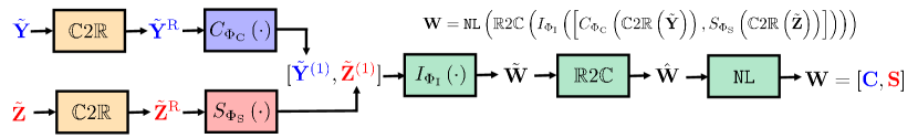
Figure 1: The proposed NN architecture.

Next, the DFBS transmits sensing waveforms. Since the target directions are not known, the sensing waveforms are selected to uniformly illuminate all angles [8]. Let ${\mathbf{E}}\in{\mathbb{C}}^{M\times L_{\rm r}}$ denote the $L_{\rm r}$-long omnidirectional waveforms transmitted from the DFBS satisfying ${{\mathbf{a}}}^{\raisebox{1.0pt}{$\rm\scriptscriptstyle H$}}(\theta)\left({\mathbf{E}}{\mathbf{E}}^{\raisebox{1.0pt}{$\rm\scriptscriptstyle H$}}\right){{\mathbf{a}}}(\theta)=c>0$ for all $\theta$. Without the loss of generality, we assume that the sensing waveforms ${\mathbf{E}}$ are orthogonal with ${\mathbf{E}}{\mathbf{E}}^{\raisebox{1.0pt}{$\rm\scriptscriptstyle H$}}=(L_{\rm r}/M){\mathbf{I}}$ with $c=L_{\rm r}$. Using (4), the received echo signals at the DFBS can be written as

$${\mathbf{Z}}=\sqrt{P_{\rm r}}\sum_{m=1}^{T}\beta_{m}{{\mathbf{g}}}_{m}^{*}{{\mathbf{g}}}_{m}^{\raisebox{1.0pt}{$\rm\scriptscriptstyle H$}}{\mathbf{E}}+{\mathbf{V}},$$ (8)

where $P_{\rm r}$ is the total transmit power of sensing waveforms and $[{\mathbf{V}}]_{i,j}\sim{\mathcal{C}}{\mathcal{N}}(0,\nu^{2})$ for all $i,j$ is the additive noise at the DFBS. The received signal is matched filtered to obtain $\tilde{{\mathbf{Z}}}\overset{\Delta}{=}{\mathbf{Z}}{\mathbf{E}}^{\raisebox{1.0pt}{$\rm\scriptscriptstyle H$}}$. We now present the proposed learning-based formulation for the transmit precoder design.

III-B Learning-based formulation

Let us denote the solution to the optimization problem $({\mathcal{P}})$ by ${\mathbf{W}}^{\star}$. Since the objective functions and the constraints are functions of the wireless channels, the optimal solution ${\mathbf{W}}^{\star}$ is also a function of the channels, i.e., ${\mathbf{W}}^{\star}=f({\mathbf{H}},{{\mathbf{g}}}_{1},\ldots,{{\mathbf{g}}}_{T})$. Moreover, since the wireless channels are estimated from the pilots and echoes, the optimal solution ${\mathbf{W}}^{\star}$ is a function of $\tilde{{\mathbf{Y}}}$ and $\tilde{{\mathbf{Z}}}$, i.e., ${\mathbf{W}}^{\star}=f_{\Phi^{\star}}(\tilde{{\mathbf{Y}}},\tilde{{\mathbf{Z}}})$, where the function $f_{\Phi}\left(\cdot\right)\colon{\mathbb{C}}^{M\times K}\times{\mathbb{C}}^{M\times M}\rightarrow{\mathbb{C}}^{M\times(M+K)}$ parameterized by $\Phi$, maps the received pilots and echoes to the solution ${\mathbf{W}}^{\star}$. Hence, $({\mathcal{P}})$ can be equivalently restated as the problem of finding the optimal parameter $\Phi^{\star}$, which is obtained by solving

$$\mathrel{\mathop{\kern 0.0pt\text{maximize}}\limits_{\Phi}} \quad Q\left(f_{\Phi}\left(\tilde{{\mathbf{Y}}},\tilde{{\mathbf{Z}}}\right)\right)$$

s. to $$\quad{\rm Tr}\left(f_{\Phi}\left(\tilde{{\mathbf{Y}}},\tilde{{\mathbf{Z}}}\right)f_{\Phi}^{\raisebox{1.0pt}{$\rm\scriptscriptstyle H$}}\left(\tilde{{\mathbf{Y}}},\tilde{{\mathbf{Z}}}\right)\right)=P_{\rm d}$$ (9a)

$$\quad\gamma_{k}\left(f_{\Phi}\left(\tilde{{\mathbf{Y}}},\tilde{{\mathbf{Z}}}\right)\right)\geq\Gamma,\,\,k=1,\ldots,K.$$ (9b)

Next, we propose an NN-based solution to solve (9).

IV The proposed NN precoder

In this section, we propose to leverage the universal function approximation [10] ability of multi-layer perceptrons to learn $f_{\Phi^{\star}}(\cdot)$ and to obtain ${\mathbf{W}}^{\star}$. That is, we seek an NN with parameters $\Phi$ for which inputs $\tilde{{\mathbf{Y}}}$ and $\tilde{{\mathbf{Z}}}$ result in an output ${\mathbf{W}}^{\star}=f_{\Phi^{\star}}(\tilde{{\mathbf{Y}}},\tilde{{\mathbf{Z}}})$ that satisfies (9a) and (9b).

IV-A The proposed NN architecture

NNs are designed to work with real-valued data. Therefore, we begin by stacking the real and imaginary parts of $\tilde{{\mathbf{Y}}}$, one below the other, in the matrix $\tilde{{\mathbf{Y}}}^{\rm R}\in{\mathbb{R}}^{2M\times K}$, where the $k$th column is given by $\tilde{{{\mathbf{y}}}}^{\rm R}_{k}=[\Re\left(\tilde{{{\mathbf{y}}}}_{k}\right)^{\raisebox{1.2pt}{$\rm\scriptstyle T$}},\Im\left(\tilde{{{\mathbf{y}}}}_{k}\right)^{\raisebox{1.2pt}{$\rm\scriptstyle T$}}]^{\raisebox{1.2pt}{$\rm\scriptstyle T$}}$. Similarly, let us define $\tilde{{\mathbf{Z}}}^{\rm R}$ with the $m$th column $\tilde{{{\mathbf{z}}}}_{m}^{\rm R}=[\Re\left(\tilde{{{\mathbf{z}}}}_{m}\right)^{\raisebox{1.2pt}{$\rm\scriptstyle T$}},\Im\left(\tilde{{{\mathbf{z}}}}_{m}\right)^{\raisebox{1.2pt}{$\rm\scriptstyle T$}}]^{\raisebox{1.2pt}{$\rm\scriptstyle T$}}$. The splitting of real and imaginary parts is carried out by the ${\mathbb{C}}2{\mathbb{R}}$ block. We process $\tilde{{\mathbf{Y}}}^{\rm R}$ and $\tilde{{\mathbf{Z}}}^{\rm R}$ through a series of MLPs to obtain ${{\mathbf{W}}}$. We begin by lifting each vector $\tilde{{{\mathbf{y}}}}_{k}^{\rm R}$ and $\tilde{{{\mathbf{z}}}}_{m}^{\rm R}$ to a higher dimension $d>2M$. To this end, we process $\tilde{{{\mathbf{y}}}}_{k}^{\rm R}$ with COMM-MLP $C_{\Phi_{\rm C}}(\cdot)\colon{\mathbb{R}}^{2M}\rightarrow{\mathbb{R}}^{d}$ to obtain $\tilde{{{\mathbf{y}}}}_{k}^{(1)}=C_{\Phi_{\rm C}}(\tilde{{{\mathbf{y}}}}_{k}^{\rm R})$ for $k=1,\ldots,K$. Similarly, we process the radar data $\tilde{{{\mathbf{z}}}}_{m}^{\rm R}$ with SENS-MLP $S_{\Phi_{\rm S}}(\cdot)\colon{\mathbb{R}}^{2M}\rightarrow{\mathbb{R}}^{d}$ to obtain $\tilde{{{\mathbf{z}}}}_{m}^{(1)}=S_{\Phi_{\rm S}}(\tilde{{{\mathbf{z}}}}_{m}^{\rm R})$ for $m=1,\ldots,M$.

Next, we process the higher dimensional representations of the communication (i.e., $\{\tilde{{{\mathbf{y}}}}_{k}^{(1)}\}_{k=1}^{K}$) and sensing data (i.e., $\{\tilde{{{\mathbf{z}}}}_{m}^{(1)}\}_{m=1}^{M}$) using ISAC-MLP, $I_{\Phi_{\rm I}}(\cdot)\colon{\mathbb{R}}^{d}\rightarrow{\mathbb{R}}^{2M}$ to obtain $K+M$ vectors of length $2M$. Let us collect the output of ISAC-MLP in a matrix $\tilde{{\mathbf{W}}}=I_{\Phi_{\rm I}}([\tilde{{{\mathbf{y}}}}_{1}^{(1)},\ldots,\tilde{{{\mathbf{y}}}}_{K}^{(1)},\tilde{{{\mathbf{z}}}}_{1}^{(1)},\ldots,\tilde{{{\mathbf{z}}}}_{M}^{(1)}])\in{\mathbb{R}}^{2M\times(M+K)}$. From $\tilde{{\mathbf{W}}}$, we construct the $M\times(M+K)$ matrix $\hat{{\mathbf{W}}}$ having complex entries using the ${\mathbb{R}}2{\mathbb{C}}$ block as $\hat{{\mathbf{W}}}=[\tilde{{\mathbf{W}}}]_{[1:M,:]}+\jmath[\tilde{{\mathbf{W}}}]_{[M+1:2M,:]}$, where the notation $\left[{\mathbf{A}}\right]_{[n:m,:]}$ refers to the submatrix obtained by collecting the rows of ${\mathbf{A}}$ with row indices $n$ to $m$. Finally, we use a normalization layer NL to obtain the transmit precoder ${\mathbf{W}}$ that satisfies (9a) as ${\mathbf{W}}=\sqrt{P_{\rm d}}\hat{{\mathbf{W}}}/\|\hat{{\mathbf{W}}}\|_{F}$. The proposed architecture is summarized in Fig. 1. Since the dimensions of the associated MLPs in the proposed NN is independent of the system parameters such as $K$, $T$, $L_{\rm p}$, or $L_{\rm r}$, the proposed method is not limited to a given setting and does not require retraining when some or all of these parameters change. Later, through numerical simulations, we demonstrate that the proposed method generalizes well across different test cases.

IV-B The loss function and training

To obtain the precoders (i.e., to learn $\Phi^{\star}$), we propose to train an NN in an unsupervised setting, since the optimal precoders (i.e., the labels) are not known beforehand during training. Typically, problems considered in unsupervised settings are unconstrained and the network is trained by minimizing a loss function. For (9), we need to choose a loss function that not only maximizes $Q(f_{\Phi}(\tilde{{\mathbf{Y}}},\tilde{{\mathbf{Z}}}))$ but also satisfy the constraints (9a) and (9b).

Let us recall that the NL block already ensures that the output satisfies (9a). However, it is not possible to carry out a similar operation on ${\mathbf{W}}$ to satisfy the SINR constraints (9b). We therefore develop a loss function that promotes outputs ${\mathbf{W}}=f_{\Phi}(\tilde{{\mathbf{Y}}},\tilde{{\mathbf{Z}}})$ that are more likely to satisfy (9b). For convenience, let us define $Q(\Phi)\overset{\Delta}{=}Q(f_{\Phi}(\tilde{{\mathbf{Y}}},\tilde{{\mathbf{Z}}}))$ and $h_{k}(\Phi)\overset{\Delta}{=}\gamma_{k}(f_{\Phi}(\tilde{{\mathbf{Y}}},\tilde{{\mathbf{Z}}}))-\Gamma$ for $k=1,\ldots,K$. Then, (9) can be rewritten as

$$\vspace{-2mm}\mathrel{\mathop{\kern 0.0pt\text{maximize}}\limits_{\Phi}}\,\,Q\left(\Phi\right)\quad\text{s. to}\quad h_{k}(\Phi)\geq 0,\,k=1,\ldots,K,$$ (10)

where we have dropped (9a) due to NL. To develop the loss function, we begin by computing the first-order optimality conditions of (10). The Lagrangian function is given by

$$L(\Phi,\boldsymbol{\mu})=Q(\Phi)+\sum_{k=1}^{K}\mu_{k}h_{k}(\Phi),$$ (11)

where $\boldsymbol{\mu}=[\mu_{1},\ldots,\mu_{K}]^{\raisebox{1.2pt}{$\rm\scriptstyle T$}}$ are the Lagrange multipliers. At the Karush-Kuhn-Tucker (KKT) optimal point $(\Phi^{\star},\boldsymbol{\mu}^{\star})$, we have

$$\nabla L(\Phi^{\star}) =\boldsymbol{0},$$ (12a)

$$h_{k}(\Phi^{\star}) \geq 0,\quad\mu_{k}^{\star}\geq 0,\quad k=1,\ldots,K$$ (12b)

$$\sum_{k=1}^{K}\mu_{k}^{\star}h_{k}(\Phi^{\star}) =0.$$ (12c)

The consequence of (12b) and (12c) on the Lagrangian can be summarized as follows. When $h_{k}(\Phi)>0$, the $k$th inequality constraint is not active. Hence, (12c) ensures that $\mu_{k}=0$, thereby ensuring $\mu_{k}h_{k}(\Phi)=0$. On the other hand, when $h_{k}(\Phi)=0$, the $k$th inequality constraint is active and $\mu_{k}\geq 0$ so that $\mu_{k}h_{k}(\Phi)=0$. Consider the following modification to (11), we have

$$\tilde{L}(\Phi,\boldsymbol{\mu})=Q(\Phi)+\sum_{k=1}^{K}|\mu_{k}|{\rm max}\left(-h_{k}(\Phi),0\right)h_{k}(\Phi)^{\kappa},$$ (13)

where $k$ is an odd number. For a feasible $(\Phi,\boldsymbol{\mu})$, the behavior of $\tilde{L}(\Phi,\boldsymbol{\mu})$ is the same as that of the $L(\Phi,\boldsymbol{\mu})$ since the second term is zero. Whenever the points are not feasible, the second term of $\tilde{L}(\Phi,\boldsymbol{\mu})$ becomes $-\sum_{k=1}^{K}|\mu_{k}|h_{k}(\Phi)^{\kappa+1}<0$.

To find the first-order optimality point, it is sufficient to learn the optimal values $\Phi^{\star}$ and $\boldsymbol{\mu}^{\star}$. To this end, we propose to train the NN with a loss-function based on $\tilde{L}(\Phi,\boldsymbol{\mu})$, i.e.,

$$\ell_{\Phi,\boldsymbol{\mu}}(\tilde{{\mathbf{Y}}},\tilde{{\mathbf{Z}}})=\lambda_{\rm S}Q(f_{\Phi}(\tilde{{\mathbf{Y}}},\tilde{{\mathbf{Z}}}))+\lambda_{\rm C}\sum_{k=1}^{K}|\mu_{k}+\epsilon|\\ \times{\rm max}(-h_{k}(f_{\Phi}(\tilde{{\mathbf{Y}}},\tilde{{\mathbf{Z}}})),0)h_{k}(f_{\Phi}(\tilde{{\mathbf{Y}}},\tilde{{\mathbf{Z}}}))^{\kappa},$$ (14)

where $\lambda_{\rm S}$, $\lambda_{\rm C}$, and $\epsilon$ are hyperparameters. We introduced $\lambda_{\rm C}$ and $\lambda_{\rm S}$ to account for the possible scale differences in the two terms in the loss function and $\epsilon$ is a small number used for numerical stability. In sum, we propose a loss function to find the first-order optimal points $(\Phi^{\star},\boldsymbol{\mu}^{\star})$ of the constrained optimization problem (10) by eliminating the constraints and absorbing them in the modified Lagrangian function.

We train the proposed NN model by minimizing the loss function $-\ell_{\Phi,\boldsymbol{\mu}}(\tilde{{\mathbf{Y}}},\tilde{{\mathbf{Z}}})$, i.e.,

$$\Phi^{\star},\boldsymbol{\mu}^{\star}=\mathrel{\mathop{\kern 0.0pt\text{argmin }}\limits_{\Phi,\boldsymbol{\mu}}}-{\mathbb{E}}\left[\ell_{\Phi,\boldsymbol{\mu}}(\tilde{{\mathbf{Y}}},\tilde{{\mathbf{Z}}})\right],$$

where the expectation is computed over different training examples of $\tilde{{\mathbf{Y}}}$ and $\tilde{{\mathbf{Z}}}$.

IV-C Complexity

The computational complexity of obtaining ${\mathbf{W}}^{\star}$ using the trained NN is as follows. Each layer of an MLP consists of a linear transformation followed by an element-wise non-linearity. Let us assume that all the MLPs comprise of an input layer, an output layer, and $L_{\rm H}$ hidden layers, each of dimension $d_{\rm H}$. Then, processing a $2M$-long vector with $C_{\Phi_{\rm C}}(\cdot)$ or $S_{\Phi_{\rm S}}(\cdot)$ costs about ${\mathcal{O}}(2Md_{\rm H}+L_{\rm H}d_{\rm H}^{2}+d_{\rm H}d)$ flops. Similarly, processing a $d$-long vector using $I_{\Phi_{\rm I}}(\cdot)$ incurs approximately ${\mathcal{O}}(dd_{\rm H}+L_{\rm H}d_{\rm H}^{2}+2Md_{\rm H})$ flops. The ${\mathbb{R}}2{\mathbb{C}}$ layer followed by NL costs about ${\mathcal{O}}(M(M+K))$ flops. Hence, the overall complexity of the NN-based solution is approximately ${\mathcal{O}}(2(M+K)(2Md_{\rm H}+L_{\rm H}d_{\rm H}^{2}+d_{\rm H}d))$ flops, which is linear in the number of users $K$. On the other hand, the complexity of the SDP-based method is ${\mathcal{O}}(M^{6.5}K^{6.5}\log(1/\delta))$, which is typically several orders higher and does not scale well with the number of UEs.

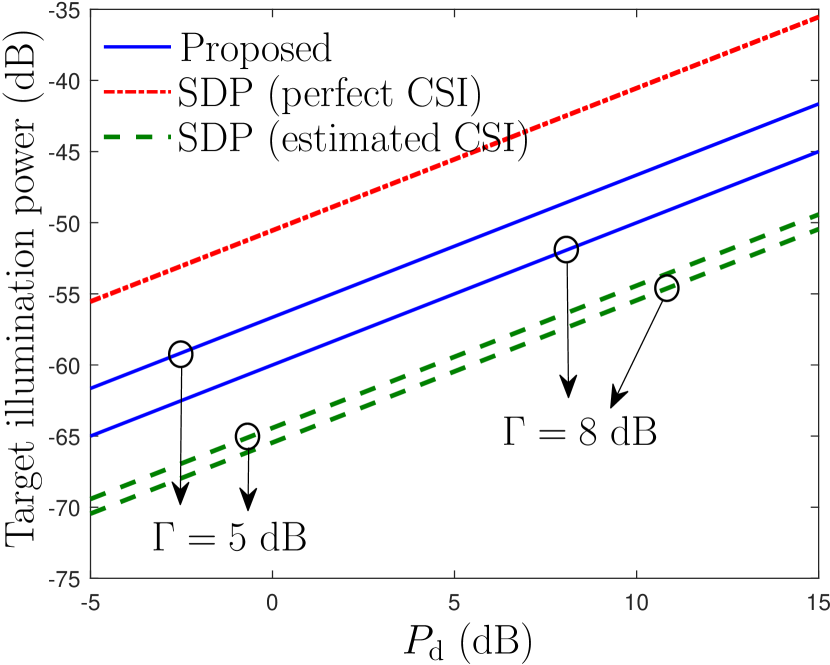
(a)

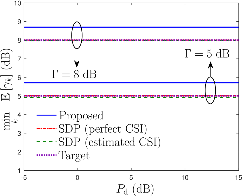
(b)

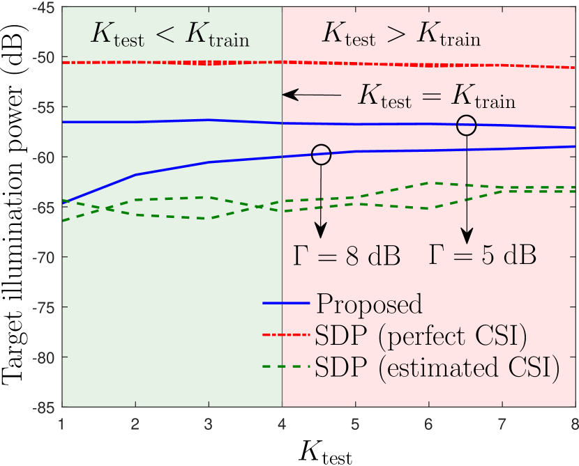
(c)

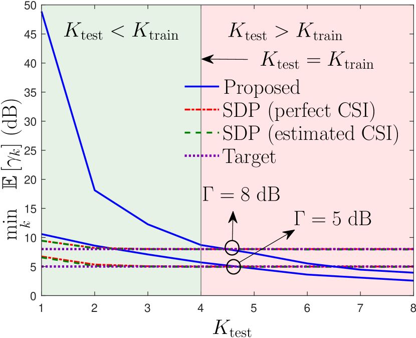
(d)

Figure 2: Impact of downlink transmit power $P_{\rm d}$: (a) Worst-case target illumination power. (b) Worst-case average SINR. Generalizability when the number of users in test set ($K_{\rm test}$) is different from the number of users used in train set ($K_{\rm train}=4$) for $P_{\rm d}=0$ dB: (c) Worst-case target illumination power. (d) Worst-case average SINR.

V Numerical simulations

We demonstrate the advantages of the proposed method through several numerical simulations. Unless otherwise mentioned, we consider $M=16$, $K=4$, $T=8$, and $\Gamma=5$ dB. We use communication pilot length and radar echo snapshots as $L_{\rm p}=20$ and $L_{\rm r}=32$, respectively. We set transmit powers as $P_{\rm r}=10$ dB and $P_{\rm u}=0$ dB. The DFBS is assumed to be at $(0,0)$m. The users are drawn with co-ordinates $(X,Y)$ where $X\in[15,18]$m, and $Y\in[8,18]$m. Targets are assumed to be located in a sector between $-80^{\circ}$ and $-10^{\circ}$ with a range of $5$ to $20$m. Communication channels are assumed to follow Rayleigh distribution with a pathloss of $30+36\log d$ dB, where $d$ is the distance of the user from the DFBS. Radar links are assumed to have a pathloss of $30+22\log d$ dB. The noise variances at the UEs and at the DFBS are selected as $\sigma^{2}=-94$ dBm and $\nu^{2}=-70$ dBm, respectively.

Both comm-MLP and Sens-MLP are two layer MLPs with the intermediate dimension being $2d$; ISAC-MLP has $4$ layers with intermediate dimensions $d$, $d$, and $2d$. All layers (except the output layer of ISAC-MLP) use ReLU activation. The output layer of ISAC-MLP is a linear layer. We train the NN for $2000$ epochs wherein each epoch comprises of $10$ batches. Each batch consists of $10$ independent realizations of $\tilde{{\mathbf{Y}}}$ and $\tilde{{\mathbf{Z}}}$. We use the hidden dimension as $d=1024$. The hyperparameters are selected through grid search as $\lambda_{\rm C}=1$, $\lambda_{\rm S}=10^{7}$, $\kappa=3$, and $\epsilon=10^{-3}$. We implement the proposed NN in Pytorch. For training, we use ADAM optimizer with a learning rate of $10^{-4}$. For training, we set $P_{\rm d}=0$ dB. We test the NN by carrying out inference over $100$ independent channel realizations.

We compare the performance of the proposed learning-based solution with that of solving $({\mathcal{P}})$ using SDP [3]. Specifically, we consider two scenarios: in the first, we assume that perfect CSI is available. We refer to this as SDP (perfect CSI). In the second scenario, we consider a more realistic situation where the underlying wireless communication channels are estimated using least-squares from $\tilde{{\mathbf{Y}}}$ and radar channel are estimated using Bartlett beamforming (for estimating $\theta_{m}$) followed by least squares (for estimating $\{\alpha_{m},\beta_{m}\}$) from $\tilde{{\mathbf{Z}}}$. We refer to this as SDP (estimated CSI).

We first evaluate the performance of the proposed method by testing the NN on a setting where the statistics of the pilots and echoes are same as the ones used during the training phase. We present the worst-case illumination power of different methods in Fig. 2(a). Throughout the considered values of $P_{\rm d}$, the performance of the proposed method is significantly better than that of SDP (estimated CSI), clearly demonstrating the advantage of using an NN to learn the precoder rather than to apply traditional optimization based techniques such as [3, 9] on estimated channels. Even though we used $P_{\rm d}=0$ dB for training, the proposed NN generalizes well across different values of $P_{\rm d}$. As $\Gamma$ increases to $8$ dB from $5$ dB, $Q$ of Proposed decrease due to more stringent communication constraints. Moreover, due to the presence of noise in $\tilde{{\mathbf{Y}}}$ and $\tilde{{\mathbf{Z}}}$, $Q$ of the Proposed will be inevitably worse than a method using perfect (noiseless) channels.

Next, we evaluate the communication performance of the proposed method by evaluating the worst-case average SINR of the UEs, $\gamma_{\rm min}=\mathrel{\mathop{\kern 0.0pt\text{min}}\limits_{k}}\quad{\mathbb{E}}\left[\gamma_{k}\right]$. If $\gamma_{\rm min}\geq\Gamma$, we conclude that the average SINR of all users are above $\Gamma$. As we can observe from Fig. 2(b), the proposed method ensures that the average SINR of all the users are higher than the desired threshold (Target) throughout the considered simulation setting. In other words, we have numerically showed that the proposed NN, along with the proposed loss function, succeeds in meeting the communication constraint in a statistical sense (i.e., on average).

To analyze the generalization capabilities of the proposed NN, we now evaluate the trained network on different scenarios, which are different from the ones used for training. We begin by presenting the communication and radar performance when the network is subjected to different UE locations in Table I.

Co-ordinates (m)	Area (m2)	$\mathrel{\mathop{\kern 0.0pt\text{min}}\limits_{k}}\,{\mathbb{E}}\left[\gamma_{k}\right]$ (dB)	$Q$ (dB)
$X\in[15,18],Y\in[8,18]$	$30$	$5.71$	$-56.73$
$X\in[10,20],Y\in[5,25]$	$200$	$6.33$	$-56.65$
$X\in[5,25],Y\in[5,25]$	$400$	$6.81$	$-56.91$

Table I: Generalizability of proposed model for different user locations $(X,Y)$ and $\Gamma=5$ dB.

The network generalizes well across different UE locations and provide consistent results even when the test area is around $10$ times larger than the locations for which the network is trained for. Next, we evaluate the performance of the proposed method on a scenario where the number of users are different in the training and testing phases. Specifically, let $K_{\rm train}=4$ and $K_{\rm test}$ denote the number of UEs during the training and testing phases, respectively. In Fig. 2(c) and Fig. 2(d), we present the worst-case target illumination power and the worst-case average SINR of the users, respectively, for different values of $K_{\rm test}$. As before, the proposed scheme clearly outperforms SDP (estimated CSI) throughout the considered range in terms of the sensing performance. Interestingly, the communication performance of Proposed is infact better whenever $K_{\rm test}<K_{\rm train}$ since the system is subjected to a simpler setting (simpler since the multi-user interference decreases when the number of users decrease) during testing than the one used during training. In general, the worst-case average SINR of Proposed decreases with an increase in $K_{\rm test}$. While $\gamma_{\rm min}<\Gamma$ for $K_{\rm test}>K_{\rm train}$, it is important to recall that we have to re-run the benchmark schemes from scratch whenever there is a change in the number of users and that the complexity of the SDP-based solution grows as $K^{6.5}$. On the other hand, the complexity of the proposed method scales linearly with the number of users (i.e, as $K$ vs $K^{6.5}$), making it much suited for next-generation massive MIMO systems.

VI Conclusions

In this paper, we proposed an NN approach to learn the transmit precoders from the received echo signals and pilots at the DFBS while avoiding the need for explicit channel estimation. The transmit precoders are designed to maximize the worst-case target illumination power while guaranteeing a prescribed SINR for the users on average. We develop a loss function based on first-order optimality conditions to train the NN model in an unsupervised setting. Through numerical simulations, we demonstrate that the proposed method outperforms traditional SDP-based methods in presence of channel estimation errors and it incurs lower computational complexity.

References

- [1] F. Liu, Y. Cui, C. Masouros, J. Xu, T. X. Han, Y. C. Eldar, and S. Buzzi, “Integrated sensing and communications: Towards dual-functional wireless networks for 6G and beyond,” IEEE J. Sel. Areas Commun., vol. 40, no. 6, pp. 1728–1767, Mar. 2022.
- [2] S. P. Chepuri, N. Shlezinger, F. Liu, G. C. Alexandropoulos, S. Buzzi, and Y. C. Eldar, “Integrated sensing and communications with reconfigurable intelligent surfaces,” arXiv preprint arXiv:2211.01003, Nov. 2022.
- [3] X. Liu, T. Huang, N. Shlezinger, Y. Liu, J. Zhou, and Y. C. Eldar, “Joint transmit beamforming for multiuser MIMO communications and MIMO radar,” IEEE Trans. Signal Process., vol. 68, pp. 3929–3944, Jun. 2020.
- [4] H. Hua, J. Xu, and T. X. Han, “Optimal transmit beamforming for integrated sensing and communication,” arXiv preprint arXiv:2104.11871, Apr. 2022.
- [5] H. Sun, X. Chen, Q. Shi, M. Hong, X. Fu, and N. D. Sidiropoulos, “Learning to optimize: Training deep neural networks for interference management,” IEEE Trans. Signal Process., vol. 66, no. 20, pp. 5438–5453, Aug. 2018.
- [6] E. Balevi, A. Doshi, and J. G. Andrews, “Massive MIMO channel estimation with an untrained deep neural network,” IEEE Trans. Wireless Commun., vol. 19, no. 3, pp. 2079–2090, Mar. 2020.
- [7] T. Jiang, H. V. Cheng, and W. Yu, “Learning to reflect and to beamform for intelligent reflecting surface with implicit channel estimation,” IEEE J. Sel. Areas Commun., vol. 39, no. 7, pp. 1931–1945, May 2021.
- [8] P. Stoica, J. Li, and Y. Xie, “On probing signal design for MIMO radar,” IEEE Trans. Signal Process., vol. 55, no. 8, pp. 4151–4161, Jul. 2007.
- [9] R. S. P. Sankar, S. P. Chepuri, and Y. C. Eldar, “Beamforming in integrated sensing and communication systems with reconfigurable intelligent surfaces,” arXiv preprint arXiv:2206.07679, Jun. 2022.
- [10] K. Hornik, M. Stinchcombe, and H. White, “Multilayer feedforward networks are universal approximators,” Neural Netw., vol. 2, no. 5, pp. 359–366, Mar. 1989.