9

Bayesian Inference of Gene Expression Dynamics in Alzheimer Brains

1 Abstract

Alzheimer’s disease (AD) is a serious neurodegenerative disease consisting of four stages where the illness gets progressively worse. It is of great significance to detect the gene regulatory mechanism as AD progresses and, thus, to help us better understand the causes of AD and find ways to treat or control AD. There are numerous researches to conduct this kind of study. However, the majority of methods are processing region by region of brain, stage by stage of AD, and then compare the results to detect changes. It is unclear how to combine these three dimensions, i.e., gene, region and stage, simultaneously to study gene expression dynamics of AD. This is the motivation of our research. In our study, we propose a statistical model of increments to clarify the relationship between gene expression in adjacent stages, so that we could better estimate the missing data we want and obtain a complete reasonable dynamic regulatory network model. Simulations are conducted to validate the statistical power of our algorithm. Moreover, a real data analysis shows that our method can capture the dynamic gene regulatory relationships among this complex brain data.

2 Introduction

Alzheimer’s disease (AD) is a slow progressing neurodegenerative disease, affecting a lot of people around the world. AD has been identified for more than a century, and although the progression of its pathologic mechanisms still remains unclear, there is increasing interest in its research (Liang et al., 2008). Significant advances have been made in understanding the neuropathological, neuroanatomical, and molecular biological abnormalities of the brains of patients with AD (Hardy, 2006). In addition, the advent of high-throughput gene expression techniques enables us to study the expression levels of multiple genes simultaneously to identify AD-related changes in many molecular biological systems (Lockhart et al., 1996).

Most cases of AD have no known genetic, and the underlying genetic modifications are complex and elusive (Bertram et al., 2010). While transcriptional studies suggest that dysfunctions of cellular pathway may precede neuropathologic markers of AD. Therefore, it is of great significance to study the changes in genetic transcription and cellular pathway of AD. There are numerous researches to conduct this kind of study. Miller et al. (2008); Miyashita, Hatsuta, Kikuchi, Nakaya, Saito, Tsukie, Hara, Ogishima, Kitamura, Akazawa, Kakita, Takahashi, Murayama, Ihara, Ikeuchi & Kuwano (2014); Shuai et al. (2013) conduct whole-genome microarray analyses through network approaches to determine transcriptional changes and gene co-expression relationships at one stage of AD or among several stages separately. In addition to the genetic changes in the brain, changes among brain regions are also causing concern. As the disease progresses, more and more brain regions are damaged, but AD does not affect all regions simultaneously or consistently (Wang et al., 2010). Some brain regions are more susceptible to AD than others (Braak & Braak, 1995). Haroutunian et al. (2009) identifies the relation between stages of AD and overall changes in gene expression, as well as the brain regions of most susceptible to transcriptional changes as the disease progressed. Wang et al. (2016) provides a comprehensive assessment of the critical molecular pathways associated with the pathology of AD by transcriptomic network analysis of 19 brain regions. However, the majority of methods are processing region by region, stage by stage, and then compare the results to detect changes. It is unclear how to combine these three dimensions, i.e., gene, region and stage, simultaneously to study genome-wide gene expression dynamics of AD, and this is our motivation.

			Stage 1	Stage 2	Stage 3	Stage 4
Person 1	Gene 1	Region 1	$\checkmark$	$\bigcirc$	$\bigcirc$	$\bigcirc$
		Region 2	$\checkmark$	$\bigcirc$	$\bigcirc$	$\bigcirc$
	Gene 2	Region 1	$\checkmark$	$\bigcirc$	$\bigcirc$	$\bigcirc$
		Region 2	$\checkmark$	$\bigcirc$	$\bigcirc$	$\bigcirc$
Person 2	Gene 1	Region 1	$\times$	$\checkmark$	$\bigcirc$	$\bigcirc$
		Region 2	$\times$	$\checkmark$	$\bigcirc$	$\bigcirc$
	Gene 2	Region 1	$\times$	$\checkmark$	$\bigcirc$	$\bigcirc$
		Region 2	$\times$	$\checkmark$	$\bigcirc$	$\bigcirc$
Person 3	Gene 1	Region 1	$\times$	$\times$	$\checkmark$	$\bigcirc$
		Region 2	$\times$	$\times$	$\times$	$\bigcirc$
	Gene 2	Region 1	$\times$	$\times$	$\checkmark$	$\bigcirc$
		Region 2	$\times$	$\times$	$\times$	$\bigcirc$

Table 1: An example to display characteristics of the brain data. There three symbols, $\checkmark$, $\times$ and $\bigcirc$, represent that the corresponding data is observed, not observed, and not produced, respectively.

In addition to considering the above three dimensions at the same time, the high missingness of the brain data is also one of the difficulties of the problem. The characteristic of the brain data is displayed in Table 1. The data was observed from brain tissue specimens derived from persons who died at specific stages of AD, thus, for a person, like Person 2 in Table 1, we can observe the data at the stage of his death, i.e. Stage 2, but we can not observe its corresponding data at Stage 1 because Person 2 was not dead yet and his brain tissue specimens were not available at Stage 1. Its corresponding data at Stage 3 can’t be observed either because the person died before Stage 3. On the other hand, not all brain regions for all persons are available on account of some aliquots from some brain regions which did not yield RNA of sufficient quality or quantity for microarray analysis, like the data of Gene 1 in Region 2 for Person 3 at Stage 3 was not observed.

Our aim is to detect gene regulatory networks of AD with different brain regions during each stage transition. In this study, a principled statistical model for brain data is proposed. A Bayesian approach is presented for estimation. A Markov chain Monte Carlo (MCMC) method, more specifically a Metropolis-within-Partially-collapsed-Gibbs algorithm, is used to draw samples from the posterior.

The remaining content of the chapter is organized as follows: the model of brain data are proposed in Section 3; the Bayesian framework is presented in Section 4; main results including simulations and real data analysis are demonstrated in Section 5 and 6, respectively; Section 7 discusses and concludes this chapter.

3 Model

In this section, a basic model of brain data is proposed.

Let $D_{g_{i}r_{j},t^{\prime}}^{e,t}$ be the data of gene $g_{i}$ in the region $r_{j}$ at stage $t^{\prime}$ for the $e$-th person who is observed at stage $t$ and $d_{g_{i}r_{j},t^{\prime}}^{e,t}$ be its corresponding value, where $t^{\prime}=1,\cdots,t$, $t=1,\cdots,T$, $i=1,\cdots,G$, $j=1,\cdots,R$, $e=1,\cdots,n_{t}$, $n_{t}$ represents the number of persons who are observed at stage $t$ and $T$, $G$, $R$ are the total number of stages, genes and regions, respectively. If $t^{\prime}=t$, $D_{g_{i}r_{j},t}^{e,t}$ is the observation, If $t^{\prime}<t$, $D_{g_{i}r_{j},t^{\prime}}^{e,t}$ is missing. At the beginning stage, i.e., $t=1$, the expression of all genes in all regions are assumed to follow Gaussian distributions with different expectations:

$$D_{g_{i}r_{j},1}^{e,t}\sim N(\mu_{g_{i}r_{j}},\sigma_{1}^{2}),\leavevmode\nobreak\ \text{for}\leavevmode\nobreak\ \left\{\begin{array}[]{lr}e=1,\cdots,n_{t}\\ t=1,\cdots,T\end{array}\right.$$

For $\sigma_{1}^{2}$, at the beginning stage of AD, the expression of most genes approach the normal situation, and with the fear of inconsistency, our model assumes that the gene expressions at the beginning stage share the same variance with different expectations. During the transition from stage $t-1$ to stage $t$, denoted as $(t-1,t)$, $t=2,\cdots,T$, there are three kinds of indicators for each $(g_{i},r_{j})$: $\gamma_{g_{i}r_{j},t-1,t}=1$ or $0$ represents $(g_{i},r_{j})$ is regulated or not, $\beta_{g_{i}r_{j},t-1,t}^{g_{m}}=1$ or $0$ represents $(g_{i},r_{j})$ is regulated by gene $g_{m}$ or not, $\beta_{g_{i}r_{j},t-1,t}^{g_{m}r_{n}}=1$ or $0$ represents $(g_{i},r_{j})$ is regulated by gene $g_{m}$ in region $r_{n}$, i.e., $(g_{m},r_{n})$, or not and there are several constraints for them: $\gamma_{g_{i}r_{j},t-1,t}+\sum_{m}\beta_{g_{i}r_{j},t-1,t}^{g_{m}}=1$ ,$\gamma_{g_{i}r_{j},t-1,t}+\sum_{n}\beta_{g_{i}r_{j},t-1,t}^{g_{m},r_{n}}=1$ for $m\neq i$ and $\gamma_{g_{i}r_{j},t-1,t}+\sum_{n\neq j}\beta_{g_{i}r_{j},t-1,t}^{g_{m},r_{n}}=1$ for $m=i$. Specifically speaking, if $\gamma_{g_{i}r_{j},t-1,t}=1$, which means $\beta_{g_{i}r_{j},t-1,t}^{g_{m}}=0$ and $\beta_{g_{i}r_{j},t-1,t}^{g_{m}r_{n}}=0$ for all other $(g_{m},r_{n})$, representing gene $g_{i}$ in the region $r_{j}$ is not regulated, then, the increment of $(g_{i},r_{j})$ from stage $t-1$ to stage $t$ follows the Gaussian distribution:

$$D_{g_{i}r_{j},t}^{e,t^{\prime}}-D_{g_{i}r_{j},t-1}^{e,t^{\prime}}\sim N(\mu_{2},\sigma_{2}^{2})\leavevmode\nobreak\ \text{for}\leavevmode\nobreak\ \left\{\begin{array}[]{lr}e=1,\cdots,n_{t^{\prime}}\\ t=2,\cdots,t^{\prime}\\ t^{\prime}=2,\cdots,T\end{array}\right.$$

If there is a unique $(g_{m},r_{n})$ to make $\beta_{g_{i}r_{j},t-1,t}^{g_{m}}=1$ and $\beta_{g_{i}r_{j},t-1,t}^{g_{m}r_{n}}=1$, representing gene $g_{i}$ in the region $r_{j}$ is regulated by gene $g_{m}$ in the region $r_{n}$, then,

$$D_{g_{i}r_{j},t}^{e,t^{\prime}}-D_{g_{i}r_{j},t-1}^{e,t^{\prime}}|D_{g_{m}r_{n},t-1}^{e,t^{\prime}}=d_{g_{m}r_{n},t-1}^{e,t^{\prime}}\sim N(a_{g_{i}r_{j},t-1,t}^{g_{m}r_{n}}+b_{g_{i}r_{j},t-1,t}^{g_{m}r_{n}}\cdot d_{g_{m}r_{n},t-1}^{e,t^{\prime}},\sigma_{2}^{2})\leavevmode\nobreak\ \text{for}\leavevmode\nobreak\ \left\{\begin{array}[]{lr}e=1,\cdots,n_{t^{\prime}}\\ t=2,\cdots,t^{\prime}\\ t^{\prime}=2,\cdots,T\end{array}\right.$$

The relationship between gene expression changes in adjacent stages is mainly used to find out the existence of regulation. Thus, for simplicity and consistency, our model assumes all increments between adjacent stages follow the same variance, $\sigma_{2}^{2}$.

4 Bayesian Inference

In this section, a Bayesian framework is proposed to estimate the parameters in the proposed model.

The joint likelihood of the complete data can be expressed as:

$$L(\bm{D}|\bm{\beta},\bm{\gamma},\bm{\mu},\bm{\sigma},\bm{a},\bm{b})=\prod_{t=1}^{T}\prod_{i=1}^{G}\prod_{j}^{R}\prod_{e=1}^{n_{t}}p(D_{g_{i}r_{j},1}^{e,t})\times\prod_{t=2}^{T}\prod_{t^{\prime}=2}^{t}\prod_{i=1}^{G}\prod_{j}^{R}\prod_{e=1}^{n_{t^{\prime}}}p(D_{g_{i}r_{j},t^{\prime}}^{e,t}-D_{g_{i}r_{j},t^{\prime}-1}^{e,t})$$

4.1 Prior

The prior distributions are as follows:

$$\mu_{g_{i}r_{j}}\sim N(c_{g_{i}r_{j}},d_{g_{i}r_{j}})$$

$$\mu_{2}\sim N(c_{2},d_{2})$$

$$\sigma^{2}_{i}\sim IG(p_{i},q_{i}),i=1,2$$

$$\gamma_{g_{i}r_{j},t-1,t},\beta_{g_{i}r_{j},t-1,t}^{g_{1}},\cdots,\beta_{g_{i}r_{j},t-1,t}^{g_{G}}\sim multinomial(\gamma_{g_{i}r_{j},t-1,t}+\sum_{m=1}^{R}\beta_{g_{i}r_{j},t-1,t}^{g_{m}}=1;\bm{p}=\frac{\bm{1}_{G}}{G})$$

$$\left\{\begin{array}[]{lr}if\ \beta_{g_{i}r_{j},t-1,t}^{g_{i}}=1:\beta_{g_{i}r_{j},t-1,t}^{g_{i}r_{1}},\cdots,\beta_{g_{i}r_{j},t-1,t}^{g_{i}r_{j-1}},\beta_{g_{i}r_{j},t-1,t}^{g_{i}r_{j+1}},\cdots,\beta_{g_{i}r_{j},t-1,t}^{g_{i}r_{R}}\\ \ \ \ \ \ \ \ \ \ \ \ \ \ \ \ \ \ \ \ \ \ \ \ \sim multinomial(\sum_{n\neq j}\beta_{g_{i}r_{j},t-1,t}^{g_{i}r_{n}}=1;\bm{p}=\frac{\bm{1}_{R-1}}{R-1})\\ if\ \beta_{g_{i}r_{j},t-1,t}^{g_{m}}=1,g_{m}\neq g_{i}:\beta_{g_{i}r_{j},t-1,t}^{g_{m}r_{1}},\cdots,\beta_{g_{i}r_{j},t-1,t}^{g_{m}r_{R}}\sim multinomial(\sum_{n=1}^{R}\beta_{g_{i}r_{j},t-1,t}^{g_{m}r_{n}}=1;\bm{p}=\frac{\bm{1}_{R}}{R})\end{array}\right.$$

$$(a_{g_{i}r_{j},t-1,t}^{g_{m}r_{n}},b_{g_{i}r_{j},t-1,t}^{g_{m}r_{n}})^{T}|\beta_{g_{i}r_{j},t-1,t}^{g_{m}r_{n}}=1\sim N(\bm{\alpha}_{g_{i}r_{j},t-1,t}^{g_{m}r_{n}},\sigma^{2}\bm{V}_{g_{i}r_{j},t-1,t}^{g_{m}r_{n}})\ and\ \sigma^{2}\sim IG(v/2,2v\lambda)$$

where $\bm{\alpha}_{g_{i}r_{j},t-1,t}^{g_{m}r_{n}}=(\alpha_{g_{i}r_{j},t-1,t}^{g_{m}r_{n},a},\alpha_{g_{i}r_{j},t-1,t}^{g_{m}r_{n},b})^{T},\bm{V}_{g_{i}r_{j},t-1,t}^{g_{m}r_{n}}=\begin{pmatrix}V_{g_{i}r_{j},t-1,t}^{g_{m}r_{n},a}&0\\ 0&v^{2}/V_{g_{i}r_{j},t-1,t}^{g_{m}r_{n},b}\end{pmatrix}$.

4.2 Posterior Inference

In this section, the detailed conditional posterior of all parameters are obtained.

4.2.1 Missing Data: $D_{g_{i}r_{j},t^{\prime}}^{e,t}$

For each observation $D_{g_{i}r_{j},t}^{e,t}$, $t\geq 2$, we estimate its corresponding missing data at all previous stages, $D_{g_{i}r_{j},t^{\prime}}^{e,t}$, $t^{\prime}=1,\cdots,t-1$, and its conditional posterior is as follows.

If $t^{\prime}=1$,

$$\begin{split}p&(D_{g_{i}r_{j},1}^{e,t}|D_{g_{i}r_{j},2}^{e,t},\bm{D}_{(-g_{i}r_{j}),1}^{e,t},\bm{D}_{(-g_{i}r_{j}),2}^{e,t},\bm{\beta},\bm{\gamma},\bm{a},\bm{b},\bm{\mu},\bm{\sigma})\\ \propto&p(D_{g_{i}r_{j},2}^{e,t}|D_{g_{i}r_{j},1}^{e,t})p(\bm{D}_{(-g_{i}r_{j}),2}^{e,t}|\bm{D}_{(-g_{i}r_{j}),1}^{e,t},D_{g_{i}r_{j},1}^{e,t})p(D_{g_{i}r_{j},1}^{e,t})\\ =&p(D_{g_{i}r_{j},2}^{e,t}-D_{g_{i}r_{j},1}^{e,t})p(\bm{D}_{(-g_{i}r_{j}),2}^{e,t}-\bm{D}_{(-g_{i}r_{j}),1}^{e,t}|D_{g_{i}r_{j},1}^{e,t})p(D_{g_{i}r_{j},1}^{e,t})\\ \Rightarrow&D_{g_{i}r_{j},1}^{e,t}|D_{g_{i}r_{j},2}^{e,t},\bm{D}_{(-g_{i}r_{j}),1}^{e,t},\bm{D}_{(-g_{i}r_{j}),2}^{e,t},\bm{\beta},\bm{\gamma},\bm{a},\bm{b},\bm{\mu},\bm{\sigma}\sim N(\frac{\mu_{miss}}{\tau^{2}_{miss}},\frac{1}{\tau^{2}_{miss}})\end{split}$$

where $\bm{D}_{(-g_{i}r_{j}),t^{\prime}}^{e,t}$ represents the complete data at stage $t^{\prime}$ of all genes in all regions of the $e$-th person observed at stage $t$, except $D_{g_{i}r_{j},t^{\prime}}^{e,t}$ and
$\mu_{miss}=\frac{E(D_{g_{i}r_{j},1}^{e,t})}{\sigma_{1}^{2}}+\frac{D_{g_{i}r_{j},2}^{e,t}-E(D_{g_{i}r_{j},2}^{e,t}-D_{g_{i}r_{j},1}^{e,t})+\sum_{(g_{m},r_{n})\neq(g_{i},r_{j})}\beta_{g_{m}r_{n},1,2}^{g_{i}r_{j}}\cdot b_{g_{m}r_{n},1,2}^{g_{i}r_{j}}(D_{g_{m}r_{n},2}^{e,t}-D_{g_{m}r_{n},1}^{e,t}-a_{g_{m}r_{n},1,2}^{g_{i}r_{j}})}{\sigma_{2}^{2}}$, $\tau^{2}_{miss}=\frac{1}{\sigma_{1}^{2}}+\frac{1+\sum_{(g_{m},r_{n})\neq(g_{i},r_{j})}\beta_{g_{m}r_{n},1,2}^{g_{i}r_{j}}\cdot(b_{g_{m}r_{n},1,2}^{g_{i}r_{j}})^{2}}{\sigma_{2}^{2}},E(D_{g_{i}r_{j},1}^{e,t})=\mu_{g_{i}r_{j}}$. For $E(D_{g_{i}r_{j},2}^{e,t}-D_{g_{i}r_{j},1}^{e,t})$, during the transition $(t=1,t=2)$, if $(g_{i},r_{j})$ is not regulated, $E(D_{g_{i}r_{j},2}^{e,t}-D_{g_{i}r_{j},1}^{e,t})=\mu_{2}$, if it is regulated by $(g_{m},r_{n})$, $E(D_{g_{i}r_{j},2}^{e,t}-D_{g_{i}r_{j},1}^{e,t})=a_{g_{i}r_{j},1,2}^{g_{m}r_{n}}+b_{g_{i}r_{j},1,2}^{g_{m}r_{n}}\cdot D_{g_{m}r_{n},1}^{e,t}$.

If $t^{\prime}\geq 2$,

$$\begin{split}p&(D_{g_{i}r_{j},t^{\prime}}^{e,t}|D_{g_{i}r_{j},t^{\prime}+1}^{e,t},D_{g_{i}r_{j},t^{\prime}-1}^{e,t},\bm{D}_{(-g_{i}r_{j}),t^{\prime}}^{e,t},\bm{D}_{(-g_{i}r_{j}),t^{\prime}+1}^{e,t},\bm{\beta},\bm{\gamma},\bm{a},\bm{b},\bm{\mu},\bm{\sigma})\\ \propto&p(D_{g_{i}r_{j},t^{\prime}}^{e,t}|D_{g_{i}r_{j},t^{\prime}-1}^{e,t})p(D_{g_{i}r_{j},t^{\prime}+1}^{e,t}|D_{g_{i}r_{j},t^{\prime}}^{e,t})p(\bm{D}_{(-g_{i}r_{j}),t^{\prime}+1}^{e,t}|\bm{D}_{(-g_{i}r_{j}),t^{\prime}}^{e,t},D_{g_{i}r_{j},t^{\prime}}^{e,t})\\ =&p(D_{g_{i}r_{j},t^{\prime}}^{e,t}-D_{g_{i}r_{j},t^{\prime}-1}^{e,t})p(D_{g_{i}r_{j},t^{\prime}+1}^{e,t}-D_{g_{i}r_{j},t^{\prime}}^{e,t})p(\bm{D}_{(-g_{i}r_{j}),t^{\prime}+1}^{e,t}-\bm{D}_{(-g_{i}r_{j}),t^{\prime}}^{e,t}|D_{g_{i}r_{j},t^{\prime}}^{e,t})\\ \Rightarrow&D_{g_{i}r_{j},t^{\prime}}^{e,t}|D_{g_{i}r_{j},t^{\prime}+1}^{e,t},D_{g_{i}r_{j},t^{\prime}-1}^{e,t},\bm{D}_{(-g_{i}r_{j}),t^{\prime}}^{e,t},\bm{D}_{(-g_{i}r_{j}),t^{\prime}+1}^{e,t},\bm{\beta},\bm{\gamma},\bm{a},\bm{b},\bm{\mu},\bm{\sigma}\sim N(\frac{\mu_{miss}}{\eta_{miss}},\frac{\sigma_{2}^{2}}{\eta_{miss}})\end{split}$$

where $\eta_{miss}=2+\sum_{(g_{m},r_{n})\neq(g_{i},r_{j})}\beta_{g_{m}r_{n},t^{\prime},t^{\prime}+1}^{g_{i}r_{j}}\cdot(b_{g_{m}r_{n},t^{\prime},t^{\prime}+1}^{g_{i}r_{j}})^{2}$, $\mu_{miss}=(D_{g_{i}r_{j},t^{\prime}-1}^{e,t}+E(D_{g_{i}r_{j},t^{\prime}}^{e,t}-D_{g_{i}r_{j},t^{\prime}-1}^{e,t}))+(D_{g_{i}r_{j},t^{\prime}+1}^{e,t}-E(D_{g_{i}r_{j},t^{\prime}+1}^{e,t}-D_{g_{i}r_{j},t^{\prime}}^{e,t}))+\sum_{(g_{m},r_{n})\neq(g_{i},r_{j})}\beta_{g_{m}r_{n},t^{\prime},t^{\prime}+1}^{g_{i}r_{j}}\cdot b_{g_{m}r_{n},t^{\prime},t^{\prime}+1}^{g_{i}r_{j}}(D_{g_{m}r_{n},t^{\prime}+1}^{e,t}-D_{g_{m}r_{n},t^{\prime}}^{e,t}-a_{g_{m}r_{n},t^{\prime},t^{\prime}+1}^{g_{i}r_{j}})$. For $E(D_{g_{i}r_{j},t^{\prime\prime}}^{e,t}-D_{g_{i}r_{j},t^{\prime\prime}-1}^{e,t}),t^{\prime\prime}=t^{\prime},t^{\prime}+1$, during the transition $(t^{\prime\prime}-1,t^{\prime\prime})$, if $(g_{i},r_{j})$ is not regulated, $E(D_{g_{i}r_{j},t^{\prime\prime}}^{e,t}-D_{g_{i}r_{j},t^{\prime\prime}-1}^{e,t})=\mu_{2}$, if it is regulated by $(g_{m},r_{n})$, $E(D_{g_{i}r_{j},t^{\prime\prime}}^{e,t}-D_{g_{i}r_{j},t^{\prime\prime}-1}^{e,t})=a_{g_{i}r_{j},t^{\prime\prime}-1,t^{\prime\prime}}^{g_{m}r_{n}}+b_{g_{i}r_{j},t^{\prime\prime}-1,t^{\prime\prime}}^{g_{m}r_{n}}\cdot D_{g_{m}r_{n},t^{\prime\prime}-1}^{e,t}$.

4.2.2 Parameters: $\mu_{g_{i}r_{j}},\sigma_{1}^{2},\mu_{2},\sigma_{2}^{2}$

For the expectations and variations, $\mu_{g_{i}r_{j}},\sigma_{1}^{2},\mu_{2},\sigma_{2}^{2}$, we have the following conditional posteriors:

$$\begin{split}p&(\mu_{g_{i}r_{j}}|\bm{D}_{g_{i}r_{j},1}^{t},t=1,\cdots,T,\sigma_{1}^{2})\propto\prod_{t=1}^{T}p(\bm{D}_{g_{i}r_{j},1}^{t}|\mu_{g_{i}r_{j}},\sigma_{1}^{2})p(\mu_{g_{i}r_{j}})\\ \Rightarrow&\mu_{g_{i}r_{j}}|\bm{D}_{g_{i}r_{j},1}^{t},t=1,\cdots,T,\sigma_{1}^{2}\sim N(\frac{\mu_{\mu_{g_{i}r_{j}}}}{\tau^{2}_{\mu_{g_{i}r_{j}}}},\frac{1}{\tau^{2}_{\mu_{g_{i}r_{j}}}})\end{split}$$

where $\mu_{\mu_{g_{i}r_{j}}}=\frac{\sum_{t=1}^{T}\sum_{e=1}^{n_{t}}D_{g_{i}r_{j},1}^{e,t}}{\sigma_{1}^{2}}+\frac{c_{g_{i}r_{j}}}{d_{g_{i}r_{j}}}$, $\tau^{2}_{\mu_{g_{i}r_{j}}}=\frac{\sum_{t=1}^{T}\sum_{e=1}^{n_{t}}1}{\sigma_{1}^{2}}+\frac{1}{d_{g_{i}r_{j}}}$ and $\bm{D}_{g_{i}r_{j},t^{\prime}}^{t}$ represents the data of gene $i$ in region $j$ at stage $t^{\prime}$ for all persons who are observed at stage $t$, i.e., $\bm{D}_{g_{i}r_{j},t^{\prime}}^{t}=\{D_{g_{i}r_{j},t^{\prime}}^{e,t};e=1,\cdots,n_{t}\}$.

$$\begin{split}p&(\sigma_{1}^{2}|\bm{D}_{1}^{t},t=2,\cdots,T,\bm{\mu})\propto\prod_{t=1}^{T}p(\bm{D}_{1}^{t}|\bm{\mu},\sigma_{1}^{2})p(\sigma_{1}^{2})\\ \Rightarrow&\sigma_{1}^{2}|\bm{D}_{1}^{t},t=1,\cdots,T,\bm{\mu}\sim IG(\alpha_{\sigma_{1}^{2}},\beta_{\sigma_{1}^{2}})\end{split}$$

where $\alpha_{\sigma_{1}^{2}}=\frac{\sum_{t=1}^{T}\sum_{i=1}^{G}\sum_{j=1}^{R}\sum_{e=1}^{n_{t}}1}{2}+p_{1}$, $\beta_{\sigma_{1}^{2}}=\frac{\sum_{t=1}^{T}\sum_{i=1}^{G}\sum_{j=1}^{R}\sum_{e=1}^{n_{t}}(D_{g_{i}r_{j},1}^{e,t}-\mu_{g_{i}r_{j}})^{2}}{2}+q_{1}$ and $\bm{D}_{t^{\prime}}^{t}$ represents the data of all gene in all region at stage $t^{\prime}$ for all persons who are observed at stage $t$, i.e., $\bm{D}_{t^{\prime}}^{t}=\{\bm{D}_{g_{i}r_{j},t^{\prime}}^{t};i=1,\cdots,G,j=1,\cdots,R\}$.

$$\begin{split}p&(\mu_{2}|\bm{D},\bm{\gamma},\sigma_{2}^{2})\propto p(\bm{D}|\bm{\gamma},\mu_{2},\sigma_{2}^{2})p(\mu_{2})\\ \Rightarrow&\mu_{2}|\bm{D},\bm{\gamma},\sigma_{2}^{2}\sim N(\frac{\mu_{\mu_{2}}}{\tau^{2}_{\mu_{2}}},\frac{1}{\tau^{2}_{\mu_{2}}})\end{split}$$

where $\mu_{\mu_{2}}=\frac{\sum_{t=2}^{T}\sum_{t^{\prime}=2}^{t}\sum_{i}^{G}\sum_{j}^{R}\sum_{e}^{n_{t}}(D_{g_{i}r_{j},t^{\prime}}^{e,t}-D_{g_{i}r_{j},t^{\prime}-1}^{e,t})\cdot\gamma_{g_{i}r_{j},t-1,t}}{\sigma_{2}^{2}}+\frac{c_{2}}{d_{2}}$, $\tau^{2}_{\mu_{2}}=\frac{\sum_{t=2}^{T}\sum_{t^{\prime}=2}^{t}\sum_{i}^{G}\sum_{j}^{R}\sum_{e}^{n_{t}}\gamma_{g_{i}r_{j},t-1,t}^{2}}{\sigma_{2}^{2}}+\frac{1}{d_{2}}$ and $\bm{D}$ represents the complete data, i.e., $\bm{D}=\{\bm{D}_{t^{\prime}}^{t};t^{\prime}=1,\cdots,t,t=1,\cdots,T\}$.

$$\begin{split}p&(\sigma_{2}^{2}|\bm{D},\bm{\beta},\bm{\gamma},\bm{a},\bm{b},\mu_{2})\propto p(\bm{D}|\bm{\beta},\bm{\gamma},\bm{a},\bm{b},\mu_{2},\sigma_{2}^{2})p(\sigma_{2}^{2})\\ \Rightarrow&\sigma_{2}^{2}|\bm{D},\bm{\beta},\bm{\gamma},\bm{a},\bm{b},\mu_{2}\sim IG(\alpha_{\sigma_{2}^{2}},\beta_{\sigma_{2}^{2}})\end{split}$$

where $\beta_{\sigma_{1}^{2}}=\frac{\sum_{t=2}^{T}\sum_{t^{\prime}=2}^{t}\sum_{i}^{G}\sum_{j}^{R}\sum_{e}^{n_{t}}(D_{g_{i}r_{j},t^{\prime}}^{e,t}-D_{g_{i}r_{j},t^{\prime}-1}^{e,t}-E(D_{g_{i}r_{j},t^{\prime}}^{e,t}-D_{g_{i}r_{j},t^{\prime}-1}^{e,t}))^{2}}{2}+q_{2}$, $\alpha_{\sigma_{2}^{2}}=\frac{\sum_{t=2}^{T}\sum_{t^{\prime}=2}^{t}\sum_{i}^{G}\sum_{j}^{R}\sum_{e}^{n_{t}}1}{2}+p_{2}$. For $E(D_{g_{i}r_{j},t^{\prime}}^{e,t}-D_{g_{i}r_{j},t^{\prime}-1}^{e,t})$, if $\gamma_{g_{i}r_{j},t^{\prime}-1,t^{\prime}}=1$, $E(D_{g_{i}r_{j},t^{\prime}}^{e,t}-D_{g_{i}r_{j},t^{\prime}-1}^{e,t})=\mu_{2}$, if $\gamma_{g_{i}r_{j},t^{\prime}-1,t^{\prime}}=0$ and $\beta_{g_{i}r_{j},t^{\prime}-1,t^{\prime}}^{g_{m}r_{n}}=1$, $E(D_{g_{i}r_{j},t^{\prime}}^{e,t}-D_{g_{i}r_{j},t^{\prime}-1}^{e,t})=a_{g_{i}r_{j},t^{\prime}-1,t^{\prime}}^{g_{m}r_{n}}+b_{g_{i}r_{j},t^{\prime}-1,t^{\prime}}^{g_{m}r_{n}}\cdot D_{g_{m}r_{n},t^{\prime}-1}^{e,t}$.

4.2.3 Coefficients: $a_{g_{i},r_{j},t-1,t}^{g_{m},r_{n}},b_{g_{i},r_{j},t-1,t}^{g_{m},r_{n}}$

Given each regulatory relationship, for its corresponding coefficients, we derive its conditional posterior and adopt MH algorithm to get its samples.

The joint prior of all coefficients is:

If $\beta_{g_{i}r_{j},t-1,t}^{g_{m}r_{n}}=1$, then, we have the following conditional priors of $a_{g_{i},r_{j},t-1,t}^{g_{m},r_{n}}$ and $b_{g_{i},r_{j},t-1,t}^{g_{m},r_{n}}$:

$$\begin{split}\sqrt{\frac{v+2N_{\beta}-1}{A_{g_{i}r_{j},t-1,t}^{g_{m}r_{n}}V_{g_{i}r_{j},t-1,t}^{g_{m}r_{n},a}}}\left(a_{g_{i}r_{j},t-1,t}^{g_{m}r_{n}}-\alpha_{g_{i}r_{j},t-1,t}^{g_{m}r_{n},a}\right)|\bm{a}_{-(g_{i}r_{j},t-1,t)},\bm{b},\bm{\beta}\sim t_{v+2N_{\beta}-1}\\ \sqrt{\frac{v+2N_{\beta}-1}{B_{g_{i}r_{j},t-1,t}^{g_{m}r_{n}}v^{2}/V_{g_{i}r_{j},t-1,t}^{g_{m}r_{n},b}}}\left(b_{g_{i}r_{j},t-1,t}^{g_{m}r_{n}}-\alpha_{g_{i}r_{j},t-1,t}^{g_{m}r_{n},b}\right)|\bm{b}_{-(g_{i}r_{j},t-1,t)},\bm{a},\bm{\beta}\sim t_{v+2N_{\beta}-1}\end{split}$$

where $\bm{a}_{-(g_{i}r_{j},t-1,t)},\bm{b}_{-(g_{i}r_{j},t-1,t)}$ represents the intercept and scale coefficients of all regulations except for the corresponding one of $(g_{i},r_{j})$ from $t-1$ to $t$, respectively, $N_{\beta}=\sum_{t,g_{i},r_{j},g_{m},r_{n}}\beta_{g_{i}r_{j},t-1,t}^{g_{m}r_{n}}$, $A_{g_{i}r_{j},t-1,t}^{g_{m}r_{n}}=\frac{(b_{g_{i}r_{j},t-1,t}^{g_{m}r_{n}}-\alpha_{g_{i}r_{j},t-1,t}^{g_{m}r_{n},b})^{2}}{v^{2}/V_{g_{i}r_{j},t-1,t}^{g_{m}r_{n},b}}+4v\lambda+C_{g_{i}r_{j},t-1,t}^{g_{m}r_{n}}$, $B_{g_{i}r_{j},t-1,t}^{g_{m}r_{n}}=\frac{(a_{g_{i},r_{j},t-1,t}^{g_{m},r_{n}}-\alpha_{g_{i}r_{j},t-1,t}^{g_{m}r_{n},a})^{2}}{V_{g_{i}r_{j},t-1,t}^{g_{m}r_{n},a}}+4v\lambda+C_{g_{i}r_{j},t-1,t}^{g_{m}r_{n}}$, and

$$\begin{split}C_{g_{i}r_{j},t-1,t}^{g_{m}r_{n}}=\sum_{t,(g_{i^{\prime}},r_{j^{\prime}})\neq(g_{i},r_{j}),g_{m^{\prime}},r_{n^{\prime}}}\beta_{g_{i^{\prime}},r_{j^{\prime}},t-1,t}^{g_{m^{\prime}},r_{n^{\prime}}}\left[\frac{(a_{g_{i^{\prime}},r_{j^{\prime}},t-1,t}^{g_{m^{\prime}},r_{n^{\prime}}}-\alpha_{g_{i^{\prime}}r_{j^{\prime}},t-1,t}^{g_{m^{\prime}}r_{n^{\prime}},a})^{2}}{V_{g_{i^{\prime}}r_{j^{\prime}},t-1,t}^{g_{m^{\prime}}r_{n^{\prime}},a}}+\frac{(b_{g_{i^{\prime}}r_{j^{\prime}},t-1,t}^{g_{m^{\prime}}r_{n^{\prime}}}-\alpha_{g_{i^{\prime}}r_{j^{\prime}},t-1,t}^{g_{m^{\prime}}r_{n^{\prime}},b})^{2}}{v^{2}/V_{g_{i^{\prime}}r_{j^{\prime}},t-1,t}^{g_{m^{\prime}}r_{n^{\prime}},b}}\right]\end{split}$$

Then, we can get the conditional posteriors of coefficients $a_{g_{i},r_{j},t-1,t}^{g_{m},r_{n}},b_{g_{i},r_{j},t-1,t}^{g_{m},r_{n}}$:

$$\begin{split}&p(a_{g_{i}r_{j},t-1,t}^{g_{m}r_{n}}|\bm{D}_{g_{i}r_{j},t}^{t^{\prime}},\bm{D}_{g_{i}r_{j},t-1}^{t^{\prime}},\bm{D}_{g_{m}r_{n},t-1}^{t^{\prime}},t^{\prime}=t,\cdots,T,b_{g_{i}r_{j},t-1,t}^{g_{m}r_{n}},\sigma_{2}^{2})\\ &\propto p\left\{\sqrt{\frac{v+2N_{\beta}-1}{A_{g_{i}r_{j},t-1,t}^{g_{m}r_{n}}V_{g_{i}r_{j},t-1,t}^{g_{m}r_{n},a}}}\left(a_{g_{i}r_{j},t-1,t}^{g_{m}r_{n}}-\alpha_{g_{i}r_{j},t-1,t}^{g_{m}r_{n},a}\right)\sim t_{v+2N_{\beta}-1}\right\}\\ &\times p\left\{a_{g_{i}r_{j},t-1,t}^{g_{m}r_{n}}\sim N(\frac{\sum_{t^{\prime}=t}^{T}\sum_{e=1}^{n_{t^{\prime}}}(D_{g_{i}r_{j},t}^{e,t^{\prime}}-D_{g_{i}r_{j},t-1}^{e,t^{\prime}}-b_{g_{i}r_{j},t-1,t}^{g_{m}r_{n}}\cdot D_{g_{m}r_{n},t-1}^{e,t^{\prime}})}{\sum_{t^{\prime}=t}^{T}\sum_{e=1}^{n_{t^{\prime}}}1},\frac{\sigma_{2}^{2}}{\sum_{t^{\prime}=t}^{T}\sum_{e=1}^{n_{t^{\prime}}}1})\right\}\\ &p(b_{g_{i}r_{j},t-1,t}^{g_{m}r_{n}}|\bm{D}_{g_{i}r_{j},t}^{t^{\prime}},\bm{D}_{g_{i}r_{j},t-1}^{t^{\prime}},\bm{D}_{g_{m}r_{n},t-1}^{t^{\prime}},t^{\prime}=t,\cdots,T,a_{g_{i}r_{j},t-1,t}^{g_{m}r_{n}},\sigma_{2}^{2})\\ &\propto p\left\{\sqrt{\frac{v+2N_{\beta}-1}{B_{g_{i}r_{j},t-1,t}^{g_{m}r_{n}}v^{2}/V_{g_{i}r_{j},t-1,t}^{g_{m}r_{n},b}}}\left(b_{g_{i}r_{j},t-1,t}^{g_{m}r_{n}}-\alpha_{g_{i}r_{j},t-1,t}^{g_{m}r_{n},b}\right)\sim t_{v+2N_{\beta}-1}\right\}\\ &\times p\left\{b_{g_{i}r_{j},t-1,t}^{g_{m}r_{n}}\sim N(\frac{\sum_{t^{\prime}=t}^{T}\sum_{e=1}^{n_{t^{\prime}}}(D_{g_{i}r_{j},t}^{e,t^{\prime}}-D_{g_{i}r_{j},t-1}^{e,t^{\prime}}-a_{g_{i}r_{j},t-1,t}^{g_{m}r_{n}})\cdot D_{g_{m}r_{n},t-1}^{e,t^{\prime}}}{\sum_{t^{\prime}=t}^{T}\sum_{e=1}^{n_{t^{\prime}}}(D_{g_{m}r_{n},t-1}^{e,t^{\prime}})^{2}},\frac{\sigma_{2}^{2}}{\sum_{t^{\prime}=t}^{T}\sum_{e=1}^{n_{t^{\prime}}}(D_{g_{m}r_{n},t-1}^{e,t^{\prime}})^{2}})\right\}\end{split}$$

4.2.4 Regulatory Relationship

For the regulatory relationship of $(g_{i},r_{j})$ during the transition $(t-1,t)$, denoted as $m^{t-1,t}_{g_{i},r_{j}}$, there are $G\times R$ situations, and only only situation will happen. Thus, this is going to involve the change in the dimension of its corresponding coefficients $a_{g_{i}r_{j},t-1,t}^{g_{m}r_{n}},b_{g_{i}r_{j},t-1,t}^{g_{m}r_{n}}$. We adopt Partially Collapsed Gibbs (PCG) sampler, which means that when we sample $m^{t-1,t}_{g_{i},r_{j}}$, its coefficients $a_{g_{i}r_{j},t-1,t}^{g_{m}r_{n}},b_{g_{i}r_{j},t-1,t}^{g_{m}r_{n}}$ are collapsed. Here is a simple example with three stages to elaborate PCG sampler:

• Parent Gibbs sampler

  • p($\bm{m}^{1,2}\leavevmode\nobreak\ |\leavevmode\nobreak\ \bm{D}_{t^{\prime}}^{t},t^{\prime}=1,2,t=2,\cdots,T,\bm{a}^{1,2},\bm{b}^{1,2},\bm{\mu},\bm{\sigma}^{2}$)

  • p($\bm{a}^{1,2},\bm{b}^{1,2}\leavevmode\nobreak\ |\leavevmode\nobreak\ \bm{m}^{1,1},\bm{D}_{t^{\prime}}^{t},t^{\prime}=1,2,t=2,\cdots,T,\bm{\mu},\bm{\sigma}^{2}$)

  • p($\bm{D}_{1}^{t},\leavevmode\nobreak\ |\leavevmode\nobreak\ \bm{m}^{1,2},\bm{D}_{2}^{t},\bm{a}^{1,2},\bm{b}^{1,2},\bm{\mu},\bm{\sigma}^{2}$) for $t=2,\cdots,T$

  • p($\bm{m}^{2,3}\leavevmode\nobreak\ |\leavevmode\nobreak\ \bm{D}_{t^{\prime}}^{t},t^{\prime}=2,3,t=3,\cdots,T,\bm{a}^{2,3},\bm{b}^{2,3},\bm{\mu},\bm{\sigma}^{2}$)

  • p($\bm{a}^{2,3},\bm{b}^{2,3}\leavevmode\nobreak\ |\leavevmode\nobreak\ \bm{m}^{2,3},\bm{D}_{t^{\prime}}^{t},t^{\prime}=2,3,t=2,\cdots,T,\bm{\mu},\bm{\sigma}^{2}$)

  • p($\bm{D}_{2}^{t}\leavevmode\nobreak\ |\leavevmode\nobreak\ \bm{m}^{1,2},\bm{m}^{2,3},\bm{D}_{1}^{t},\bm{D}_{3}^{t},\bm{a}^{2,3},\bm{b}^{2,3},\bm{\mu},\bm{\sigma}^{2}$) for $t=3,\cdots,T$

  • p($\bm{\mu},\bm{\sigma}^{2}\leavevmode\nobreak\ |\leavevmode\nobreak\ \bm{m},\bm{ab},\bm{\mu},\bm{\sigma}^{2},\bm{D}$)

• Partially Collapsed Gibbs sampler

  • p($\bm{m}^{1,2}\leavevmode\nobreak\ |\leavevmode\nobreak\ \bm{D}_{t^{\prime}}^{t},t^{\prime}=1,2,t=2,\cdots,T,\bm{\mu},\bm{\sigma}^{2}$)

  • p($\bm{a}^{1,2},\bm{b}^{1,2}\leavevmode\nobreak\ |\leavevmode\nobreak\ \bm{m}^{1,1},\bm{D}_{t^{\prime}}^{t},t^{\prime}=1,2,t=2,\cdots,T,\bm{\mu},\bm{\sigma}^{2}$)

  • p($\bm{D}_{1}^{t},\leavevmode\nobreak\ |\leavevmode\nobreak\ \bm{m}^{1,2},\bm{D}_{2}^{t},\bm{a}^{1,2},\bm{b}^{1,2},\bm{\mu},\bm{\sigma}^{2}$) for $t=2,\cdots,T$

  • p($\bm{m}^{2,3}\leavevmode\nobreak\ |\leavevmode\nobreak\ \bm{D}_{t^{\prime}}^{t},t^{\prime}=2,3,t=3,\cdots,T,\bm{\mu},\bm{\sigma}^{2}$)

  • p($\bm{a}^{2,3},\bm{b}^{2,3}\leavevmode\nobreak\ |\leavevmode\nobreak\ \bm{m}^{2,3},\bm{D}_{t^{\prime}}^{t},t^{\prime}=2,3,t=2,\cdots,T,\bm{\mu},\bm{\sigma}^{2}$)

  • p($\bm{D}_{2}^{t}\leavevmode\nobreak\ |\leavevmode\nobreak\ \bm{m}^{1,2},\bm{m}^{2,3},\bm{D}_{1}^{t},\bm{D}_{3}^{t},\bm{a}^{2,3},\bm{b}^{2,3},\bm{\mu},\bm{\sigma}^{2}$) for $t=3,\cdots,T$

  • p($\bm{\mu},\bm{\sigma}^{2}\leavevmode\nobreak\ |\leavevmode\nobreak\ \bm{m},\bm{ab},\bm{\mu},\bm{\sigma}^{2},\bm{D}$)

We can find that the PCG sampler avoids the use of reversible jump MCMC algorithm by marginalizing over the coefficient whose dimension is not fixed. For the inference of indicators $\gamma_{g_{i}r_{j},t-1,t}$ and $\beta_{g_{i}r_{j},t-1,t}^{g_{m}r_{n}}$, let’s get the conditional posterior of $\sigma^{2}$ first:

$$\begin{split}p&(\sigma^{2}|\bm{a}_{-(g_{i}r_{j},t-1,t)},\bm{b}_{-(g_{i}r_{j},t-1,t)},\bm{\beta})\propto p(\bm{a}_{-(g_{i}r_{j},t-1,t)},\bm{b}_{-(g_{i}r_{j},t-1,t)}|\bm{\beta},\sigma^{2})p(\sigma^{2})\\ \propto&(\sigma^{2})^{-(\frac{v}{2}+1)}e^{-\frac{2v\lambda}{\sigma^{2}}}(\sigma^{2})^{-\sum_{t,(g_{i^{\prime}},r_{j^{\prime}})\neq(g_{i},r_{j}),g_{m^{\prime}},r_{n^{\prime}}}\beta_{g_{i^{\prime}},r_{j^{\prime}},t-1,t}^{g_{m^{\prime}},r_{n^{\prime}}}}\\ \times&\exp\left\{-\frac{1}{2\sigma^{2}}\sum_{t,(g_{i^{\prime}},r_{j^{\prime}})\neq(g_{i},r_{j}),g_{m^{\prime}},r_{n^{\prime}}}\beta_{g_{i^{\prime}},r_{j^{\prime}},t-1,t}^{g_{m^{\prime}},r_{n^{\prime}}}\left[\frac{(a_{g_{i^{\prime}},r_{j^{\prime}},t-1,t}^{g_{m^{\prime}},r_{n^{\prime}}}-\alpha_{g_{i^{\prime}}r_{j^{\prime}},t-1,t}^{g_{m^{\prime}}r_{n^{\prime}},a})^{2}}{V_{g_{i^{\prime}}r_{j^{\prime}},t-1,t}^{g_{m^{\prime}}r_{n^{\prime}},a}}+\frac{(b_{g_{i^{\prime}}r_{j^{\prime}},t-1,t}^{g_{m^{\prime}}r_{n^{\prime}}}-\alpha_{g_{i^{\prime}}r_{j^{\prime}},t-1,t}^{g_{m^{\prime}}r_{n^{\prime}},b})^{2}}{v^{2}/V_{g_{i^{\prime}}r_{j^{\prime}},t-1,t}^{g_{m^{\prime}}r_{n^{\prime}},b}}\right]\right\}\\ \Rightarrow&\sigma^{2}|\bm{a}_{-(g_{i}r_{j},t-1,t)},\bm{b}_{-(g_{i}r_{j},t-1,t)},\bm{\beta}\sim IG(\frac{v}{2}+N_{\beta,g_{i}r_{j},t-1,t}^{g_{m}r_{n}},2v\lambda+\frac{1}{2}C_{g_{i}r_{j},t-1,t}^{g_{m}r_{n}})\end{split}$$

where $N_{\beta,g_{i}r_{j},t-1,t}^{g_{m}r_{n}}=\sum_{t,(g_{i^{\prime}},r_{j^{\prime}})\neq(g_{i},r_{j}),g_{m^{\prime}},r_{n^{\prime}}}\beta_{g_{i^{\prime}},r_{j^{\prime}},t-1,t}^{g_{m^{\prime}},r_{n^{\prime}}}$.

Thus, for the data $\bm{D}_{g_{i}r_{j},t}^{t^{\prime}},t^{\prime}\geq t$, we have:

where $\bm{\mu}=\bm{X}_{g_{m}r_{n},t-1}^{(t-T)}\bm{\alpha}_{g_{i}r_{j},t-1,t}^{g_{m}r_{n}}$,$\bm{\Sigma}=\frac{4v\lambda+C_{\beta,g_{i}r_{j},t-1,t}^{g_{m}r_{n}}}{v+2N_{\beta,g_{i}r_{j},t-1,t}^{g_{m}r_{n}}}(\sigma_{2}^{2}\bm{I}+\bm{X}_{g_{m}r_{n},t-1}^{(t-T)}\bm{V}_{g_{i}r_{j},t-1,t}^{g_{m}r_{n}}(\bm{X}_{g_{m}r_{n},t-1}^{(t-T)})^{T})$, $\bm{X}_{g_{m}r_{n},t-1}^{(t-T)}=(\bm{1},\bm{D}_{g_{m}r_{n},t-1}^{(t-T)})$, and $\bm{D}_{g_{i}r_{j},t^{\prime}}^{(t-T)}=\begin{pmatrix}\bm{D}_{g_{i}r_{j},t^{\prime}}^{(t)}\\ \bm{D}_{g_{i}r_{j},t^{\prime}}^{(t+1)}\\ \cdots\\ \bm{D}_{g_{i}r_{j},t^{\prime}}^{(T)}\end{pmatrix}$.

Thus, for $(g_{i},r_{j})$, its parameters $\gamma_{g_{i}r_{j},t-1,t},\beta_{g_{i}r_{j},t-1,t}^{g_{m}},\beta_{g_{i}r_{j},t-1,t}^{g_{m}r_{n}}$ satisfy:

4.3 Algorithm

The basic steps of the whole algorithm are shown in Algorithm 1.

Algorithm 1 Algorithm for Brain Data

0:    The observation $\bm{D}_{t}^{t},t=1,\cdots,T$;The initial regulatory relationships $\bm{M}^{t-1,t}_{0},t=2,\cdots,T$

0:    The new regulatory relationships during each stage transition $\bm{M}^{t-1,t},t=2,\cdots,T$;The missing data $\bm{D}_{t^{\prime}}^{t},t^{\prime}=1,\cdots,t,t=2,\cdots,T$;All other parameters $\bm{\mu},\bm{\sigma}$;

1:  for $t=2;t\leq T;t++$ do

2:     for $l=1;l\leq L;l++$ do

3:        propose a candidate model $\bm{M}^{t-1,t}_{*}\sim g(\bm{M}|\bm{M}^{t-1,t}_{l-1})$ according to some proposal distribution g

4:        calculate acceptance rate: $\theta=\min(\frac{p(\bm{M}^{t-1,t}_{*}|\bm{D})}{p(\bm{M}^{t-1,t}_{l-1}|\bm{D})}\cdot\frac{g(\bm{M}^{t-1,t}_{l-1}|\bm{M}^{t-1,t}_{*})}{g(\bm{M}^{t-1,t}_{*}|\bm{M}^{t-1,t}_{l-1})},1)$

5:        sample $u\sim U(0,1)$

6:        if $u<\theta$ then

7:           accept the proposal $\bm{M}^{t-1,t}_{l}=\bm{M}^{t-1,t}_{*}$

8:        else

9:           Reject the proposal $\bm{M}^{t-1,t}_{l}=\bm{M}^{t-1,t}_{l-1}$

10:        end if

11:        update $\bm{a},\bm{b}$

12:     end for

13:     let $\bm{M}^{t-1,t}=\bm{M}^{t-1,t}_{L}$

14:     sample the missing data $\bm{D}_{t-1}^{t}\leavevmode\nobreak\ |\leavevmode\nobreak\ \bm{M}^{t^{\prime}-1,t^{\prime}},\bm{D}_{t^{\prime\prime}}^{t^{\prime}},t^{\prime\prime}\leq t^{\prime}-2,t^{\prime}\leq T,\bm{a},\bm{b},\bm{\mu},\bm{\sigma^{2}}$

15:  end for

16:  sample $(\bm{\mu},\bm{\sigma^{2}})\leavevmode\nobreak\ |\leavevmode\nobreak\ \bm{M},\bm{D},\bm{a},\bm{b}$

For the production of the proposal model $\bm{M}^{t-1,t}_{*}$ based on a given model $\bm{M}^{t-1,t}_{l-1}$, there are three alternative operations to conduct which are described in Algorithm 2,3,4. Moreover, to show the connection between regions for the same gene, when we sample a different $(g_{m},r_{n})$ for $(g_{i},r_{j})$, we are going to sample $g_{m}$ first, and then sample $r_{n}$.

Algorithm 2 Adding a regulatory relationship (Add)

0:    A regulatory model $\bm{M}^{t-1,t}$ with at least one gene in one region which is not regulated

0:    A new regulatory mode $\bm{M}^{t-1,t}_{*}$

1:  find all genes and regions which are not regulated in $\bm{M}^{t-1,t}$, denoted as set $\{(g_{i}^{\prime},r_{j}^{\prime})\}$ with $\gamma_{g_{i}^{\prime}r_{j}^{\prime},t-1,t}=1$

2:  calculate the posterior probability $p(\gamma_{g_{i}^{\prime}r_{j}^{\prime},t-1,t}=1|\bm{D},\bm{\mu},\bm{\sigma},\bm{b},\bm{a})$

3:  sample a $(g_{i}*,r_{j}*)$ in set $\{(g_{i}^{\prime},r_{j}^{\prime})\}$ with the probability proportional to $1-p(\gamma_{g_{i}^{\prime}r_{j}^{\prime},t-1,t}=1|\bm{D},\bm{\mu},\bm{\sigma},\bm{b},\bm{a})$

4:  calculate the posterior probability $p(\beta_{g_{i}*r_{j}*,t-1,t}^{g_{m}^{\prime}r_{n}^{\prime}}=1|\bm{D},\bm{\mu},\bm{\sigma},\bm{b},\bm{a})$ for all $(g_{m}^{\prime},r_{n}^{\prime})\neq(g_{i}*,r_{j}*)$

5:  sample a $(g_{m}*,r_{n}*)$ in set $\{(g_{m}^{\prime},r_{n}^{\prime})\neq(g_{i}*,r_{j}*)\}$ with the probability proportional to $p(\beta_{g_{i}*r_{j}*,t-1,t}^{g_{m}^{\prime}r_{n}^{\prime}}=1|\bm{D},\bm{\mu},\bm{\sigma},\bm{b},\bm{a})$

6:  generate a new model $\bm{M}^{t-1,t}_{*}$ by making $\beta_{g_{i}*r_{j}*,t-1,t}^{g_{m}*r_{n}*}=1$

Algorithm 3 Deleting a regulatory relationship (Delete)

0:    A regulatory model $\bm{M}^{t-1,t}$ with at least one regulatory relationship

0:    A new regulatory mode $\bm{M}^{t-1,t}_{*}$

1:  find all regulatory relationships in $\bm{M}^{t-1,t}$ denoted as set $\{(g_{i}^{\prime},r_{j}^{\prime},g_{m}^{\prime},r_{n}^{\prime})\}$ which means $\beta_{g_{i}^{\prime}r_{j}^{\prime},t-1,t}^{g_{m}^{\prime}r_{n}^{\prime}}=1$

2:  calculate the posterior probability $p(\beta_{g_{i}^{\prime}r_{j}^{\prime},t-1,t}^{g_{m}^{\prime}r_{n}^{\prime}}=1|\bm{D},\bm{\mu},\bm{\sigma},\bm{b},\bm{a})$

3:  sample a $(g_{i}*,r_{j}*,g_{m}*,r_{n}*)$ in set $\{(g_{i}^{\prime},r_{j}^{\prime},g_{m}^{\prime},r_{n}^{\prime})\}$ with the probability proportional to $1-p(\beta_{g_{i}*r_{j}*,t-1,t}^{g_{m}*r_{n}*}=1|\bm{D},\bm{\mu},\bm{\sigma},\bm{b},\bm{a})$

4:  generate a new model $\bm{M}^{t-1,t}_{*}$ by making $\gamma_{g_{i}*r_{j}*,t-1,t}=1$

Algorithm 4 Swapping a regulatory relationship (Swap)

0:    A regulatory model $\bm{M}^{t-1,t}$

0:    A new regulatory mode $\bm{M}^{t-1,t}_{*}$

1:  find all regulatory relationships in $\bm{M}^{t-1,t}$ denoted as set $\{(g_{i}^{\prime},r_{j}^{\prime},g_{m}^{\prime},r_{n}^{\prime})\}$ which means $\beta_{g_{i}^{\prime}r_{j}^{\prime},t-1,t}^{g_{m}^{\prime}r_{n}^{\prime}}=1$

2:  calculate the posterior probability $p(\beta_{g_{i}^{\prime}r_{j}^{\prime},t-1,t}^{g_{m}^{\prime}r_{n}^{\prime}}=1|\bm{D},\bm{\mu},\bm{\sigma},\bm{b},\bm{a})$

3:  sample a $(g_{i}*,r_{j}*,g_{m}*,r_{n}*)$ in set $\{(g_{i}^{\prime},r_{j}^{\prime},g_{m}^{\prime},r_{n}^{\prime})\}$ with the probability proportional to $1-p(\beta_{g_{i}*r_{j}*,t-1,t}^{g_{m}*r_{n}*}=1|\bm{D},\bm{\mu},\bm{\sigma},\bm{b},\bm{a})$

4:  calculate the posterior probability $p(\beta_{g_{i}*r_{j}*,t-1,t}^{g_{m}^{\prime\prime}r_{n}^{\prime\prime}}=1|\bm{D},\bm{\mu},\bm{\sigma},\bm{b},\bm{a})$ for all $(g_{m}^{\prime\prime},r_{n}^{\prime\prime})\neq(g_{i}*,r_{j}*)$

5:  sample a $(g_{m}**,r_{n}**)$ in set $\{(g_{m}^{\prime\prime},r_{n}^{\prime\prime})\neq(g_{i}*,r_{j}*)\text{ and }(g_{m}*,r_{j}*)\}$ with the probability proportional to $p(\beta_{g_{i}*r_{j}*,t-1,t}^{g_{m}^{\prime\prime}r_{n}^{\prime\prime}}=1|\bm{D},\bm{\mu},\bm{\sigma},\bm{b},\bm{a})$

6:  generate a new model $\bm{M}^{t-1,t}_{*}$ by making $\beta_{g_{i}*r_{j}*,t-1,t}^{g_{m}*r_{n}*}=0$ and $\beta_{g_{i}*r_{j}*,t-1,t}^{g_{m}**r_{n}**}=1$

5 Simulation Results

In this section, large scale simulations are performed to validate our algorithm for brain data.

To synthesize the data, the underlying true parameter values are fixed, 100 networks are randomly generated with the same $G=5,R=5,T=4$ as the underlying true regulatory relationships. For each of the 100 parameter settings, one dataset with 20 observations at each stage is generated from the proposed model. And other experimental settings are given in Appendix A.1 in detail.

For comparison, other three simple methods, denoted as Pearson1, Pearson2 and Pearson3, respectively, through Pearson correlation coefficient are adopted and its basic steps are described in Algorithm 5. Pearson1 only use the observation dataset to estimate the networks, but Pearson2 and Pearson3 conduct missing data imputation firstly before estimating the networks, moreover, not only imputing $\times$, but $\bigcirc$ in Table1. For Pearson2, the missing data is estimated by the mean value of its corresponding observations, for instance, the estimators of missing $D_{g_{i}r_{j},t^{\prime}}^{e,t}$, $t^{\prime}\neq t$, for all $e=1,\cdots,n_{t}$ and $t=1,\cdots,T$ are the same and equal to the mean value of the observations $\bm{D}_{g_{i}r_{j},t^{\prime}}^{t^{\prime}}$. For Pearson3, we obtain the complete dataset by Random Forest Missing Data Algorithm (Tang & Ishwaran, 2017). Table 2 shows the simulation results.

There are four evaluation indexes adopted to assess the performances. The ‘Detection’ represents the ratio of number of regulatory relationships detected to number of regulatory relationships in true networks. The ‘Recall’ represents the ratio of number of regulatory relationships correctly detected to number of regulatory relationships in true networks. The ‘Error’ represents the ratio of total learning error (false positives plus false negatives) to number of regulatory relationships in true networks. The ’$F_{1}$ score’ represents the ratio $2\cdot\frac{\text{Precision}\cdot\text{Recall}}{\text{Precision}+\text{Recall}}$.

As shown in Table 2, no matter what the index, no matter what the stage, the proposed approach is far better than other methods. To be more specific, our ‘Detection’s are closer to 1 than the others and our ‘Recall’s are superior to all others indicating that our method not only is very accurate, also have fewer false positive. Thus, our ‘Error’s are much smaller and ‘$F_{1}$ score’s are much larger than all others. However, relatively speaking, our method does not perform very well during the first stage transition. This phenomenon is understandable and explicable. During each stage transition, both its corresponding observations and missing data are used to learn its network. For the first stage transition, the missing data accounts for $(T-1)\times 100$% and they are furthest from their corresponding observations, making them the most difficult to estimate, thus, the missing data affects the estimation accuracy to some extent.

Algorithm 5 Algorithm for Pearson1, Pearson2 and Pearson3

0:    If Pearson1, input the observation $\bm{D}_{t}^{t},t=1,\cdots,T$;If Pearson2 or Pearson 3, input the complete dataset $\bm{D}$ after imputation

0:    The regulatory networks

1:  for $t=2;t\leq T;t++$ do

2:     for $g_{i}=1;g_{i}\leq G;g_{i}++$ do

3:        for $r_{j}=1;r_{j}\leq R;r_{j}++$ do

4:           If Pearson1, calculate Pearson correlation coefficients between $(\bm{D}_{g_{i}r_{j},t-1}^{t-1},\bm{D}_{g_{i}r_{j},t}^{t})$ and $(\bm{D}_{g_{m}r_{n},t-1}^{t-1},\bm{D}_{g_{i}r_{j},t}^{t})$ for all $(g_{m},r_{n})\neq(g_{i},r_{j})$;If Pearson2 or Pearson 3, calculate Pearson correlation coefficients between $\{\bm{D}_{g_{i}r_{j},t}^{t^{\prime}};t^{\prime}=1,\cdots,T\}$ and $\{\bm{D}_{g_{m}r_{n},t}^{t^{\prime}};t^{\prime}=1,\cdots,T\}$ for all $(g_{m},r_{n})\neq(g_{i},r_{j})$

5:           if all correlation coefficients are smaller than 0.5 then

6:              $(g_{i},r_{j})$ is not regulated during $(t-1,t)$

7:           else

8:              $(g_{i},r_{j})$ is regulated by $(g_{m},r_{n})$ with largest absolute value of correlation coefficient during $(t-1,t)$

9:           end if

10:        end for

11:     end for

12:  end for

Table 2: Results of simulations for detecting regulatory relationships. Each row represents one evaluation index during one stage transition or the whole transition and each column indicates one method. The values in brackets are the variations of the corresponding indexes.

		Pearson 1	Pearson 2	Pearson 3	Proposed
Stage 1 $\rightarrow$ 2	Detection	1.1857 (0.4228)	4.1251 (9.7894)	4.0321 (9.1675)	1 (0.023)
	Recall	0.0353 (0.012)	0.0058 (0.0019)	0.0058 (0.0019)	0.5239 (0.1237)
	Error	1.3004 (0.4182)	4.9458 (9.9604)	4.8646 (9.3752)	0.4875 (0.1471)
	$F_{1}$ score	0.0476 (0.0209)	0.0036 (7e-04)	0.004 (9e-04)	0.6083 (0.1264)
Stage 2 $\rightarrow$ 3	Detection	1.3238 (0.8217)	6.4895 (20.3016)	6.4597 (20.863)	0.9932 (0.0041)
	Recall	0.0258 (0.009)	0.0103 (0.0039)	0.0103 (0.0039)	0.7199 (0.1)
	Error	1.5181 (0.8867)	7.1702 (20.3729)	7.144 (20.9782)	0.2824 (0.1038)
	$F_{1}$ score	0.0308 (0.0118)	0.0037 (5e-04)	0.0038 (5e-04)	0.784 (0.0899)
Stage 3 $\rightarrow$ 4	Detection	1.9853 (1.5127)	6.6772 (23.1663)	6.5436 (22.1384)	1.1044 (0.1947)
	Recall	0.0537 (0.0158)	0.0088 (0.0023)	0.0098 (0.0025)	0.7326 (0.1107)
	Error	2.1129 (2.0116)	7.2945 (22.5546)	7.1683 (21.699)	0.3884 (0.3237)
	$F_{1}$ score	0.0578 (0.0189)	0.004 (5e-04)	0.0045 (5e-04)	0.762 (0.0942)
Total	Detection	1.4324 (0.1251)	4.4902 (2.0268)	4.4241 (2.0042)	1.008 (0.0097)
	Recall	0.0414 (0.0041)	0.0092 (0.0011)	0.0099 (0.0012)	0.6662 (0.0331)
	Error	1.4746 (0.128)	5.1945 (2.0181)	5.1311 (2.0082)	0.3551 (0.04)
	$F_{1}$ score	0.0533 (0.0071)	0.0038 (2e-04)	0.0041 (2e-04)	0.7759 (0.0221)

6 Real Data Analyses

We apply our method on a real dataset about genome-wide gene expression provided by (Haroutunian et al., 2009). The brain is divided into 19 regions and the progress of AD is stratified into 4 stages according to the density of cerebrocortical neuritic plaque. The higher the stage, the more severe the disease. A microarray analysis in human postmortem specimens was conducted by Gene Logic Inc. using Affymetrix. Data from 992 samples were normalized using MAS 5.0 algorithms and $\text{GX}^{\text{TM}}$ Explorer v.2.0 (Katsel et al., 2005). The brain dataset handling procedures are described in detail by (Haroutunian et al., 2009) and sample distributions of the data between different regions are shown in Appendix A.2. These are the 19 regions: Anterior Cingulate (AC), Caudate Nucleus (CN), Dorsolateral Prefrontal Cortex (DPC), Frontal Pole (FP), Hippocampus (HIP), Inferior Frontal Gyrus (IFG), Inferior Temporal Gyrus (ITG), Middle Temporal Gyrus (MTG), Occipital Visual Cortex (OVC), Parahippocampal Gyrus (ParaG), Posterior Cingulate Cortex (PCC), Precentral Gyrus (PreG), Prefrontal Cortex (PC), Putamen (PUT), Superior Parietal Lobule (SPL), Superior Temporal Gyrus (STG), Temporal Pole (TP), Amygdala (Amyg), Nucleus Accumbens (NA).

In the previous simulations with 5 genes, 5 regions and 4 stages, it takes 6.182 hours for 10000 MCMC iterations. Because of the property of MCMC and the exponentially increasing of the number of possible regulatory relationships with the numbers of genes and regions, our algorithm may take a pretty long time when the number of genes or regions is very large. Thus, we suggest practical approaches to use our MCMC algorithm under are two situations to perform the real data analysis.

The first situation is that the numbers of genes and regions that we’re interested in are not very large. In this case, we can conduct one MCMC experiment to get the result. In this experiment, specific regions and genes are selected to demonstrate the rationality of our method. Five regions are selected: PC, HIP, MTG, STG, PG. PC is part of the frontal lobe, and it contributes to working memory (Boisgueheneuc et al., 2006). HIP is associated with short-term, long-term memory and spatial memory (Suthana et al., 2012). MTG, STG and PG are the three regions with the greatest changes in gene expression (Haroutunian et al., 2009). Fifteen genes are selected: $PHYHD1$, $MYO5C$, $ENPP2$, $MOG$, $GPR37$, $LIPA$, $MAG$, $PSEN1$, $TF$, $BIN1$, $CR1$, $SORL1$, $CASS4$, $CLU$, $PICALM$. These genes can be divided into three categories. It is likely that functional failure of $PHYHD1$ and $MYO5C$ could lead to AD development (Miyashita, Hatsuta, Kikuchi, Nakaya, Saito, Tsukie, Hara, Ogishima, Kitamura, Akazawa et al., 2014). Seven genes, $ENPP2$, $MOG$, $GPR37$, $LIPA$, $MAG$, $PSEN1$, $TF$, are in the same module which is related to disease progression (Miller et al., 2008). And the last six genes are associated with AD in genome-wide significance (Lambert et al., 2013). In this real data analysis with 15 genes and 5 regions, it takes 21.133 hours for 10000 MCMC iterations. The results are shown in Table 3.

Table 3: Results of real data for detecting regulatory relationships. Each $g_{i},r_{j}-g_{m},r_{n}$ represents one detected regulatory relationship and means that gene $g_{i}$ in region $r_{j}$ is regulated by gene $g_{m}$ in region $r_{n}$ during the corresponding stage transition, and the value in bracket is the proportion of this regulatory relationship in its corresponding MCMC samples. The indexes of regions, 1 to 5, correspond to PC, HIP, MTG, STG and PG in turn. The indexes of genes, 1 to 15, correspond to $PHYHD1$, $MYO5C$, $ENPP2$, $MOG$, $GPR37$, $LIPA$, $MAG$, $PSEN1$, $TF$, $BIN1$, $CR1$, $SORL1$, $CASS4$, $CLU$, $PICALM$ in turn.

Stage transition	Detected regulatory relationships
Stage 1 $\rightarrow$ 2	$\begin{matrix}\\ 3,2-5,2(21.50\%)&4,2-8,2(21.60\%)&4,5-7,5(18.40\%)\\ 6,5-4,5(38.64\%)\\ \\ \end{matrix}$
Stage 2 $\rightarrow$ 3	$\begin{matrix}\\ \\ \end{matrix}$
Stage 3 $\rightarrow$ 4	$\begin{matrix}\\ 2,5-13,4(26.59\%)&4,3-11,1(21.89\%)&4,5-11,1(18.06\%)\\ 5,2-13,4(15.43\%)&9,3-12,1(25.30\%)&11,4-10,4(21.12\%)\\ 12,1-11,5(24.19\%)&13,4-2,5(20.58\%)&15,1-13,5(21.75\%)\\ \\ \end{matrix}$

In Table 3, we can find that, during the first stage transition, all detected regulatory relationships exist within the same module mentioned above. During the last stage transition, genes in the third category are involved most, which confirms their significance in relation to AD. Thus, this real data analysis shows that our method can reach conclusions that align well with existing biological knowledge.

The another situation is that the numbers of genes or regions are so large that one MCMC experiment may not handle them. The following procedure, Algorithm 6, is proposed to detect the regulatory relationships with wide ranges of genes or regions. This algorithm is essentially a dimensionality reduction method, but genes and regions may overlap in different MCMC, thus, we can try to ensure that every possible situation maybe considered if the MCMC is used enough times. Based on the computational times in the simulation and first real data analysis, we can obviously find that this kind of procedure is pretty necessary for wide ranges of genes and regions, otherwise, one MCMC experiment might take too long to get the result. In this experiment, we adopt all regions and randomly select 100 genes to conduct the second real data analysis and we set $N_{M}=10$, $G=15$, $R=5$. The full result is displayed in Appendix A.3 and its corresponding index tables of genes and regions are provided in Appendix A.4. The total computational time is 219.345 hours.

Algorithm 6 Algorithm for brain data with wide ranges of genes or regions

0:    $N_{G}$ genes; $N_{R}$ regions; $T$ stages$G$: number of genes within one MCMC; $R$: number of regions within one MCMC; $N_{M}$: times of MCMC

0:    The regulatory networks

1:  for $g_{i}=1;g_{i}\leq N_{G};g_{i}++$ do

2:     Calculate the Pearson correlation coefficients between $\{\bm{D}_{g_{i}r_{j},t}^{t};t=1,\cdots,T,r_{j}=1,\cdots,N_{R}\}$ and $\{\bm{D}_{g_{m}r_{n},t}^{t};t=1,\cdots,T,r_{n}=1,\cdots,N_{R}\}$ for all $g_{m}\neq g_{i}$, denoted as $Cor_{g_{i}}^{g_{m}}$;

3:  end for

4:  for $r_{j}=1;r_{j}\leq N_{R};r_{j}++$ do

5:     Conduct the hypothesis test: $H_{0}:D_{g_{i}r_{j},t}^{t}=D_{g_{m}r_{n},t}^{t}$ VS $H_{1}:D_{g_{i}r_{j},t}^{t}\neq D_{g_{m}r_{n},t}^{t}$ for all $(g_{i},r_{j})$, $t\geq 2$ and denote its p-value as $P_{g_{i}r_{j}}^{t}$;

6:  end for

7:  for $m_{t}=1;m_{t}\leq N_{M};m_{t}++$ do

8:     Sample $G$ genes from the whole $N_{G}$ genes without replacement according to the probability of $g_{i}$ satisfying: $P(g_{i})\propto\sum_{g_{m}\neq g_{i}}Cor_{g_{i}}^{g_{m}}$;

9:     Sample $R$ regions from the whole $N_{R}$ regions without replacement according to the probability of $r_{j}$ satisfying: $P(r_{j})\propto\#\{P_{g_{i}r_{j}}^{t}<=0.05;t=2,\cdots,T,g_{i}=1,\cdots,N_{G}\}$;

10:     Input the $G$ genes and $R$ regions into Algorithm 1;

11:  end for

7 Conclusion

In this study, a full Bayesian framework is proposed to detect gene regulatory relationships of AD brain during each stage transition. Simulations are conducted to validate the statistical power of our algorithm. Moreover, a real data analysis shows that our method can capture the gene regulatory relationships among this complex brain data.

The majority of other methods to identify gene regulatory relationships or analysis transcriptional changes are processing region by region of brain, stage by stage of AD, and then compare these sub-results to detect relationships or changes. However, such approach would lack the integrity of regions and the coherence of stages. We present an overall statistical model of regulatory relationships in AD, thus, we can deal with gene, region and stage, these three dimensions, simultaneously to study genome-wide gene expression dynamics.

Our model and algorithm can also be applied to other areas. For example, dynamic network learning with time dimension, it can also degenerate into static network learning.

Even so, there are still some problems to be solved. For instance, the regulatory mechanism in the model is relatively simple, and more complex cases need further research. The relationship between regions is not reflected in the model. And the computational power of algorithms also needs to be improved. These will be the focus of our future work.

Appendix

A.1 Experimental Settings for Brain Data

We used the following hyper-parameters for the prior distributions:

$$c_{g_{i}r_{j}}=5,d_{g_{i}r_{j}}=0.5$$

$$c_{2}=0,d_{2}=0.5$$

$$p_{i}=3,q_{i}=2,\text{ for }i=1,2$$

$$\bm{\alpha}_{g_{i}r_{j},t-1,t}^{g_{m}r_{n}}=\begin{pmatrix}1\\ 1\end{pmatrix},\bm{V}_{g_{i}r_{j},t-1,t}^{g_{m}r_{n}}=\begin{pmatrix}1&0\\ 0&1\end{pmatrix}$$

$$v=2,\lambda=0.05$$

for all possible $(g_{i},r_{j})$, $(g_{m},r_{n})$ and $t$.

The matrix of probability function of alternative operations to the modes is given as follows:

No Relationship100All Regulated00.80.2Other Case0.30.40.3)fragments No Relationship100All Regulated00.80.2Other Case0.30.40.3\left(\left.\begin{tabular}[]{c|c|c|c}Model Type&Add&Delete&Swap\\ \hline\cr No Relationship&1&0&0\\ \hline\cr All Regulated&0&0.8&0.2\\ \hline\cr Other Case&0.3&0.4&0.3\end{tabular}\right.\right)

Model TypeAddDeleteSwapModel TypeAddDeleteSwap

A.2 Sample Distributions for Brain Data

For the gene expression of each person, we calculate its sample distribution characteristics, i.e., standard deviation, median, mean, 1st and 3rd quantiles, based on the observations of all genes. For each region and each stage, we put the observations of all genes and its all corresponding persons together to plot its box plot. The results are shown in Figure A.1 and Figure A.2, respectively. We can find that the distributions of gene expression in different gene chips are similar after normalization.

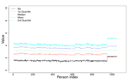
Figure A.1: Sample distribution characteristics of All Persons for brain data.

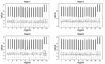
Figure A.2: Box plots of the sample distributions in different regions for brain data. Each box plot shows the sample distribution corresponding to a same region.

A.3 Results of Brains data with Wide Range of Genes and Regions

Table A.1: Results of real data for detecting regulatory relationships with wide range of genes and regions. Each $g_{i},r_{j}-g_{m},r_{n}$ represents one detected regulatory relationship and means that gene $g_{i}$ in region $r_{j}$ is regulated by gene $g_{m}$ in region $r_{n}$ during the corresponding stage transition, and the value in bracket is the proportion of this regulatory relationship in its corresponding MCMC samples.

Stage transition	Detected regulatory relationships
Stage 1 $\rightarrow$ 2	$\begin{matrix}\\ 1,8-92,3(50.93\%)&1,18-26,10(48.21\%)&1,19-92,8(50.00\%)\\ 5,6-16,16(23.33\%)&9,14-11,11(31.18\%)&11,1-37,5(39.17\%)\\ 12,16-24,16(46.41\%)&15,12-98,1(48.35\%)&15,19-36,12(37.52\%)\\ 18,16-18,12(47.72\%)&20,8-92,3(50.00\%)&20,18-76,16(48.24\%)\\ 27,4-68,3(50.86\%)&27,7-94,18(40.46\%)&29,1-53,1(42.16\%)\\ 29,12-53,17(39.37\%)&33,3-23,19(27.00\%)&33,12-92,8(50.15\%)\\ 36,12-92,1(37.87\%)&36,19-62,8(45.55\%)&39,19-71,19(18.54\%)\\ 40,1-40,19(50.00\%)&43,16-50,18(39.62\%)&43,18-94,7(27.58\%)\\ 43,18-66,10(50.21\%)&43,19-96,8(28.52\%)&48,19-92,8(50.00\%)\\ 50,7-87,18(49.27\%)&51,18-49,8(50.77\%)&53,17-64,15(25.04\%)\\ 57,18-66,10(18.46\%)&61,18-74,7(23.89\%)&62,1-98,1(50.00\%)\\ 62,12-40,3(39.49\%)&62,17-76,17(34.35\%)&63,7-41,3(49.30\%)\\ 63,17-63,12(43.52\%)&63,18-94,7(50.17\%)&64,16-58,16(21.50\%)\\ 65,18-65,2(19.05\%)&68,16-33,4(44.89\%)&70,19-71,19(31.58\%)\\ 74,18-31,16(29.88\%)&81,18-10,16(31.82\%)&88,2-61,18(21.99\%)\\ 91,11-73,11(50.00\%)&92,8-98,1(50.76\%)&92,12-33,3(50.00\%)\\ 96,3-33,12(28.08\%)&96,18-63,16(41.63\%)&98,19-20,1(56.54\%)\\ 99,18-66,11(22.23\%)\\ \\ \end{matrix}$
Stage 2 $\rightarrow$ 3	$\begin{matrix}\\ 3,16-88,16(50.06\%)&9,6-11,1(49.82\%)&11,14-56,19(44.36\%)\\ 16,6-11,2(38.39\%)&16,14-11,14(39.03\%)&16,15-53,12(40.25\%)\\ 26,11-61,14(36.41\%)&31,1-18,16(49.66\%)&32,2-91,11(33.95\%)\\ 43,10-49,1(37.88\%)&43,18-68,16(38.79\%)&43,18-97,1(36.58\%)\\ 44,6-69,16(48.20\%)&44,9-65,13(50.03\%)&45,11-20,14(39.04\%)\\ 50,10-66,18(34.20\%)&51,4-13,1(31.22\%)&51,9-55,9(30.28\%)\\ 51,19-41,9(50.00\%)&53,1-53,16(38.19\%)&56,1-65,10(50.00\%)\\ 56,19-11,14(39.12\%)&58,16-73,15(50.00\%)&61,6-11,16(48.47\%)\\ 61,16-88,16(50.00\%)&63,1-18,16(48.08\%)&63,10-65,13(50.00\%)\\ 67,16-63,1(50.00\%)&70,6-13,19(34.14\%)&70,14-11,19(35.11\%)\\ 72,18-49,1(38.42\%)&76,17-53,16(46.30\%)&78,19-71,16(42.04\%)\\ 80,6-56,6(27.01\%)&81,6-60,16(33.44\%)&81,14-70,16(40.66\%)\\ 82,10-88,16(50.07\%)&82,16-22,14(29.40\%)&87,1-3,16(50.00\%)\\ 89,13-73,2(35.29\%)&90,6-11,1(50.41\%)&96,1-36,3(43.64\%)\\ 97,11-57,1(25.77\%)&99,10-49,1(50.02\%)&99,11-97,8(20.95\%)\\ \\ \end{matrix}$

Table A.2: Results of real data for detecting regulatory relationships with wide range of genes and regions (continued Figure A.1).

Stage transition

Detected regulatory relationships

Stage 3 $\rightarrow$ 4

$\begin{matrix}\\ 1,12-44,3(16.00\%)&3,16-88,16(26.04\%)&5,6-22,6(11.19\%)\\ 9,2-56,2(13.76\%)&9,11-11,11(22.29\%)&11,2-20,2(26.35\%)\\ 11,10-88,2(14.86\%)&13,18-81,18(35.70\%)&16,17-54,12(18.45\%)\\ 18,5-20,2(28.85\%)&18,15-69,17(15.00\%)&18,16-63,17(29.49\%)\\ 20,1-36,1(16.40\%)&20,2-18,5(26.70\%)&20,2-88,13(09.92\%)\\ 20,12-36,3(31.99\%)&20,19-36,12(51.27\%)&21,1-62,17(11.26\%)\\ 21,15-54,15(20.06\%)&21,17-58,12(22.19\%)&21,19-26,4(09.48\%)\\ 23,1-48,12(31.45\%)&24,5-31,7(18.42\%)&24,13-88,13(16.91\%)\\ 24,16-65,16(17.02\%)&24,16-61,16(11.32\%)&25,2-20,10(12.57\%)\\ 25,11-20,14(14.65\%)&27,3-41,4(10.17\%)&27,7-91,3(11.88\%)\\ 29,15-16,15(18.37\%)&29,16-53,1(28.94\%)&31,7-24,5(21.97\%)\\ 31,18-69,16(14.99\%)&32,2-88,2(16.74\%)&32,13-88,2(19.72\%)\\ 36,1-20,1(18.31\%)&36,3-20,12(29.96\%)&36,12-20,19(52.79\%)\\ 36,19-48,1(11.61\%)&37,1-69,1(27.17\%)&37,6-69,16(28.83\%)\\ 39,10-89,11(13.92\%)&39,11-11,14(15.03\%)&41,16-13,19(06.42\%)\\ 43,10-49,1(16.14\%)&43,18-89,18(19.55\%)&44,1-96,3(31.38\%)\\ 44,9-64,10(08.35\%)&45,11-53,14(13.40\%)&45,15-62,12(40.92\%)\\ 48,12-23,1(28.48\%)&49,1-49,8(18.15\%)&50,10-89,11(24.62\%)\\ 51,10-89,1(16.20\%)&53,1-29,16(27.21\%)&53,2-56,14(14.06\%)\\ 53,12-18,15(27.94\%)&56,1-71,16(09.11\%)&56,9-88,1(18.58\%)\\ 56,13-45,11(11.97\%)&58,16-63,3(10.01\%)&58,16-63,12(50.00\%)\\ 59,9-24,1(29.02\%)&59,10-63,13(13.92\%)&59,16-63,10(49.07\%)\\ 60,10-59,10(16.00\%)&60,16-24,16(14.86\%)&61,14-9,13(20.25\%)\\ 61,16-64,9(20.86\%)&62,8-20,3(16.84\%)&62,12-45,15(44.75\%)\\ 62,17-21,12(22.81\%)&63,1-67,16(43.92\%)&63,10-59,16(49.44\%)\\ 63,12-58,16(57.33\%)&64,1-69,12(13.40\%)&64,15-63,16(09.59\%)\\ 65,9-87,10(19.58\%)&65,10-71,16(09.40\%)&66,11-89,8(18.14\%)\\ 67,1-87,10(22.92\%)&67,9-56,13(11.65\%)&67,16-63,1(47.88\%)\\ 68,16-76,7(19.25\%)&69,1-37,1(26.98\%)&69,1-66,10(25.89\%)\\ 71,4-13,4(08.44\%)&72,1-49,11(15.47\%)&72,8-49,8(13.95\%)\\ 72,10-49,10(15.05\%)&73,2-20,10(19.41\%)&73,10-56,11(18.61\%)\\ 73,17-69,17(31.77\%)&76,4-58,7(13.88\%)&76,7-68,16(19.58\%)\\ 76,7-13,2(19.82\%)&78,19-13,4(10.11\%)&80,8-57,10(20.02\%)\\ 80,10-97,11(45.97\%)&81,18-13,18(35.14\%)&82,6-22,2(07.04\%)\\ 82,10-87,9(05.76\%)&82,19-13,1(06.66\%)&87,1-65,10(10.02\%)\\ 87,10-67,1(25.84\%)&88,1-64,9(17.45\%)&88,2-32,2(18.04\%)\\ 88,10-91,2(23.54\%)&88,13-24,13(34.94\%)&88,14-61,14(10.14\%)\\ 88,16-56,9(15.43\%)&89,10-90,10(28.59\%)&89,18-50,8(34.24\%)\\ 90,1-50,10(11.29\%)&91,10-39,10(18.97\%)&96,3-44,1(27.81\%)\\ 97,11-80,10(46.07\%)&98,8-62,3(16.72\%)&99,8-80,10(16.76\%)\\ 99,10-49,8(31.32\%)&99,11-1,10(32.62\%)\\ \end{matrix}$

A.4 The indexes of Genes and Regions in Brain Data

Table A.3: Index table of regions in Brain data.

Index	1	2	3
Region	Anterior Cingulate	Caudate Nucleus	Dorsolateral Prefrontal Cortex
Index	4	5	6
Region	Frontal Pole	Hippocampus	Inferior Frontal Gyrus
Index	7	8	9
Region	Inferior Temporal Gyrus	Middle Temporal Gyrus	Occipital Visual Cortex
Index	10	11	12
Region	Parahippocampal Gyrus	Posterior Cingulate Cortex	Precentral Gyrus
Index	13	14	15
Region	Prefrontal Cortex	Putamen	Superior Parietal Lobule
Index	16	17	18
Region	Superior Temporal Gyrus	Temporal Pole	Amygdala
Index	19
Region	Nucleus Accumbens

Table A.4: Index table of genes in Brain data.

Index	1	2	3	4	5	6	7	8
Region	phyhd1	myo5c	enpp2	mog	gpr37	lipa	mag	psen1
Index	9	10	11	12	13	14	15	16
Region	tf	bin1	cr1	sorl1	cass4	clu	picalm	ash2l
Index	17	18	19	20	21	22	23	24
Region	lyn	tchp	aqp4	prickle3	kiaa0494	ecscr	znf282	fxyd3
Index	25	26	27	28	29	30	31	32
Region	ccl11	gpr172a	scg5	c1orf107	cdkn2a	itgam	map3k9	pde9a
Index	33	34	35	36	37	38	39	40
Region	ip6k2	upp1	sh3gl3	sprr1a	trappc9	diras2	hace1	ddx3x
Index	41	42	43	44	45	46	47	48
Region	upk1a	capn1	hs6st2	cyb5d1	phf6	cwc27	loc100507448	nmi
Index	49	50	51	52	53	54	55	56
Region	fgf8	slco3a1	rab14	u2af1	loc100506318	ncrna00158	c16orf46	loc100506305
Index	57	58	59	60	61	62	63	64
Region	chchd6	tlr6	nrg4	c10orf95	slc35e1	loc100509703	slc35a3	hdac2
Index	65	66	67	68	69	70	71	72
Region	nucb1	dpf3	ltn1	nox3	adam1	ttll7	shc4	fam114a2
Index	73	74	75	76	77	78	79	80
Region	cd160	enpp1	las1l	nudt4	cldn14	cgrrf1	kbtbd8	aoc2
Index	81	82	83	84	85	86	87	88
Region	loc401052	phf1	sh2b1	sry	loc100507619	nedd9	iqsec2	rfwd2
Index	89	90	91	92	93	94	95	96
Region	wdr72	fezf2	ebf4	ncoa3	egr3	loc100128496	pvt1	fign
Index	97	98	99	100
Region	tubb1	loc283624	bloc1s2	plekhh2

References

- (1)
- Bertram et al. (2010) Bertram, L., Lill, C. M. & Tanzi, R. E. (2010), ‘The genetics of Alzheimer’s disease: Back to the future’, Neuron 68(2), 270–281.
- Boisgueheneuc et al. (2006) Boisgueheneuc, F. d., Levy, R., Volle, E., Seassau, M., Duffau, H., Kinkingnehun, S., Samson, Y., Zhang, S. & Dubois, B. (2006), ‘Functions of the left superior frontal gyrus in humans: a lesion study’, Brain 129(12), 3315–3328.
- Braak & Braak (1995) Braak, H. & Braak, E. (1995), ‘Staging of Alzheimer’s disease-related neurofibrillary changes.’, Neurobiology of Aging 16(3), 271–278.
- Hardy (2006) Hardy, J. (2006), ‘A hundred years of Alzheimer’s disease research.’, Neuron 52(1), 3–13.
- Haroutunian et al. (2009) Haroutunian, V., Katsel, P. & Schmeidler, J. (2009), ‘Transcriptional vulnerability of brain regions in Alzheimer’s disease and dementia’, Neurobiology of Aging 30(4), 561–573.
- Katsel et al. (2005) Katsel, P., Davis, K. L., Gorman, J. M. & Haroutunian, V. (2005), ‘Variations in differential gene expression patterns across multiple brain regions in schizophrenia’, Schizophrenia Research 77(2-3), 241–252.
- Lambert et al. (2013) Lambert, J.-C., Ibrahim-Verbaas, C. A., Harold, D., Naj, A. C., Sims, R., Bellenguez, C., Jun, G., DeStefano, A. L., Bis, J. C., Beecham, G. W. et al. (2013), ‘Meta-analysis of 74,046 individuals identifies 11 new susceptibility loci for Alzheimerś disease’, Nature genetics 45(12), 1452–1458.
- Liang et al. (2008) Liang, W. S., Dunckley, T., Beach, T. G., Grover, A. & Stephan, D. A. (2008), ‘Neuronal gene expression in non-demented individuals with intermediate Alzheimer’s disease neuropathology’, Neurobiology of Aging 31(4), 549–566.
- Lockhart et al. (1996) Lockhart, D. J., Dong, H., Byrne, M. C., Follettie, M. T., Gallo, M. V., Chee, M. S., Mittmann, M., Wang, C., Kobayashi, M. & Norton, H. (1996), ‘Expression monitoring by hybridization to high-density oligonucleotide arrays’, Nature Biotechnology 14(13), 1675–1680.
- Miller et al. (2008) Miller, J. A., Oldham, M. C. & Geschwind, D. H. (2008), ‘A systems level analysis of transcriptional changes in Alzheimer’s disease and normal aging’, Journal of Neuroscience the Official Journal of the Society for Neuroscience 28(6), 1410–1420.
- Miyashita, Hatsuta, Kikuchi, Nakaya, Saito, Tsukie, Hara, Ogishima, Kitamura, Akazawa, Kakita, Takahashi, Murayama, Ihara, Ikeuchi & Kuwano (2014) Miyashita, A., Hatsuta, H., Kikuchi, M., Nakaya, A., Saito, Y., Tsukie, T., Hara, N., Ogishima, S., Kitamura, N., Akazawa, K., Kakita, A., Takahashi, H., Murayama, S., Ihara, Y., Ikeuchi, T. & Kuwano, R. (2014), ‘Genes associated with the progression of neurofibrillary tangles in Alzheimer’s disease’, Translational Psychiatry 4, 1–8.
- Miyashita, Hatsuta, Kikuchi, Nakaya, Saito, Tsukie, Hara, Ogishima, Kitamura, Akazawa et al. (2014) Miyashita, A., Hatsuta, H., Kikuchi, M., Nakaya, A., Saito, Y., Tsukie, T., Hara, N., Ogishima, S., Kitamura, N., Akazawa, K. et al. (2014), ‘Genes associated with the progression of neurofibrillary tangles in Alzheimerś disease’, Translational psychiatry 4(6), 1–8.
- Shuai et al. (2013) Shuai, H., Jing, L., Jieping, Y., Adam, F., Kewei, C., Teresa, W. & Eric, R. (2013), ‘A sparse structure learning algorithm for gaussian bayesian network identification from high-dimensional data’, IEEE Trans Pattern Anal Mach Intell 35(6), 1328–42.
- Suthana et al. (2012) Suthana, N., Haneef, Z., Stern, J., Mukamel, R., Behnke, E., Knowlton, B. & Fried, I. (2012), ‘Memory enhancement and deep-brain stimulation of the entorhinal area’, New England Journal of Medicine 366(6), 502–510.
- Tang & Ishwaran (2017) Tang, F. & Ishwaran, H. (2017), ‘Random forest missing data algorithms’, Statistical Analysis and Data Mining 10(6), 363–377.
- Wang et al. (2016) Wang, M., Roussos, P., Mckenzie, A., Zhou, X., Kajiwara, Y., Brennand, K. J., De Luca, G. C., Crary, J. F., Casaccia, P. & Buxbaum, J. D. (2016), ‘Integrative network analysis of nineteen brain regions identifies molecular signatures and networks underlying selective regional vulnerability to Alzheimer’s disease’, Genome Medicine 8(1), 1–21.
- Wang et al. (2010) Wang, X., L. Michaelis, M. & K. Michaelis, E. (2010), ‘Functional genomics of brain aging and Alzheimer’s disease: Focus on selective neuronal vulnerability’, Current Genomics 11(8), 618–633.