Chapter 1 Kinetic Helicity in the Earth’s atmosphere

   Michael Kurgansky

[1]Otto Chkhetiani

Abstract

An overview is given of the helicity of the velocity field (“kinetic” helicity to distinguish it from the “magnetic” helicity used in magnetohydrodynamics, astrophysics, and solar physics; or simply helicity in this Chapter) and of the role, which this concept plays in the modern research in atmospheric physics and atmospheric turbulence. General information on helicity is presented including some historical comments and a brief description of the fundamental role that helicity plays in fluid dynamics. Different applications of the helicity concept are discussed to the analysis of various dynamic atmospheric processes, including applications to intense atmospheric vortices, such as tropical cyclones, tornadoes and dust devils, and also to Ekman boundary layer dynamics. Emphasized are helicity balance conditions and the important role that helicity fluxes play in their maintenance. Fundamentals of helical turbulence theory are briefly discussed, and then emphasis is placed on the helical properties of atmospheric turbulence within the atmospheric boundary layer. In particular, the pioneering effort of the research team from the Obukhov Institute of Atmospheric Physics (Moscow) to measure turbulent helicity in natural atmospheric conditions is described.

Keywords: atmospheric dynamics, helicity, turbulence

1.1 Introduction

This Chapter addresses the notion of “kinetic helicity”, or simply helicity, and its various applications to atmospheric dynamics and atmospheric turbulence. Helicity, or more precisely the helicity bulk density, is defined by a dot product $\displaystyle h=\mathbf{v}\cdot{\bm{\omega}}$ of the three-dimensional velocity $\displaystyle\mathbf{v}$ and vorticity $\displaystyle{\bm{\omega}=}\bm{\nabla}\times\mathbf{v}$ vectors. It is a pseudoscalar quantity, that is, its sign depends on the chosen frame of reference, either right-handed or left-handed, and this sign changes to the opposite under mirror reflection. Helicity is positive when air parcels move along a helical line following the right hand rule. On the contrary, the air motion according to the left hand rule corresponds to negative helicity.

There is a certain hierarchy of atmospheric motions with respect to vorticity: (i) irrotational (potential) flows, (i) rotational flows (vortices), both two-dimensional and three-dimensional but with zero helicity in the latter case, and (iii) helical vortex flows, which are inherently three-dimensional, generally have a complex topology of the vorticity field, and which, in a certain sense, are at the top rung of this hierarchical ladder. In meteorology and atmospheric physics, the interest of many researchers in the concept of helicity is mainly explained by its importance for the study of atmospheric vortex flows, which are usually, but not always, of the convective origin and have a complex structure, sometimes topologically non-trivial. These include tornadoes and dust devils, (e.g., Tippett et al., 2014; Smith et al., 2014; Clark et al., 2012, 2013); tropical mesoscale vortices (Shenming et al., 2011) and tropical cyclones (e.g., Levina et al., 2009; Molinari and Vollaro, 2010; Yu and Yu, 2011; Levina, 2019; Chen et al., 2021); and turbulence (e.g., Chkhetiani and Golbraikh, 2012; Yu et al., 2013; Rorai et al., 2013; Chkhetiani et al., 2018; Vazaeva et al., 2017, 2021). Less attention has been paid to the helicity of large-scale extratropical atmospheric motions, explained by atmospheric barocilinicity and Earth’s rotation (Etling, 1985; Kurgansky, 1990; Bluestein, 1992).

This Chapter has the following structure. Section 1.2 provides an overview of helicity, including some historical comments, and presents a brief overview of the fundamental role that helicity plays in fluid dynamics. The different applications of the concept of helicity to the analysis of various dynamic atmospheric processes are discussed in Section 1.3. The fundamentals of the theory of helical turbulence are briefly discussed in Section 1.4, and then the helical properties of atmospheric turbulence within the atmospheric boundary layer. In particular, the pioneering effort of the research team of the Obukhov Institute of Atmospheric Physics (Moscow) to measure turbulent helicity under natural atmospheric conditions is described. Final Section 1.5 presents the concluding remarks and formulates the problems that are resisted in the theory of helical turbulence.

1.2 Generalities (general information on helicity)

In the basic fluid dynamics, the conservation law of helicity for barotropic flows of non-viscous fluids in the presence of only potential external forces was discovered by Moreau (1961) and Moffatt (1969) two centuries after L. Euler presented in 1757 his famous equations of the fluid motion. Moffatt (1969) clarified the topological meaning of helicity as a measure of linkage (knottedness) of vortex lines. This helicity conservation law and its interpretation are closely related to demands of the famous circulation theorem by Lord Kelvin (1868), who as noted in Moffatt (1969) was fully aware of the possibility of the existence of linked and knotted vortex lines. These ideas go back to the classic works of C.F. Gauss on electromagnetism.

Actually, J-J. Moreau [1961] and K. Moffatt [1969] had more immediate predecessors, among them H. Ertel, who in a joint article with C.-G. Rossby (Ertel and Rossby, 1949) derived the local conservation law for ideal barotropic flows of a compressible fluid,

$$\frac{{\rm D}}{{\rm D}t}\left\{\frac{1}{\rho}\bm{\omega}\cdot\left(\mathbf{v}-\bm{\nabla}W\right)\right\}=0,W=\int\limits_{0}^{t}{\cal L}dt.$$ (1.1)

Here, $\displaystyle{{\rm D}/{\rm D}t}$ denotes the total (material) derivative in time. Under the integral sign along the fluid particle trajectory, such that $\displaystyle{\cal L}={{\rm D}W/{\rm D}t}$, stands the fluid dynamical Lagrange function, with $\displaystyle\rho$ as the fluid density, $\displaystyle p$ the pressure and $\displaystyle\Phi$ the gravity potential,

$${\cal L}=\frac{\mathbf{v}^{2}}{2}-\left(\Phi+\int\frac{dp}{\rho}\right).$$

The law of conservation of total (integral) helicity follows immediately from (1.1) if to multiply it by $\displaystyle\rho$ and integrate over the domain occupied by the fluid motion, given that the boundary of the domain is not penetrated by the vortex lines.

Helicity is not a Galilean invariant quantity; see, for example, Bluestein (1992). There is an analogy with neutrino physics (note how Moffatt (1969) proposed the term “helicity” by analogy with the neutrino), where the helicity sign of the neutrino depends on the reference frame in which a neutrino with a non-zero rest mass is observed, that is, moving slower or faster than the neutrino (Goldhaber and Goldhaber, 2011). The same situation is possible in atmospheric physics. In tornado research, helicity is usually considered in the reference frame associated with the paternal storm, within which a tornado originates. Moving on to another Galilean frame of reference, a situation can be achieved in which, for example, the right rotation of the wind with height (so called in meteorology, because an observer who stands facing the wind discovers that the wind at a higher level blows from the right side, e.g., Koschmieder (1933)), corresponding to positive helicity, will be changed (locally) to left rotation, corresponding to negative helicity.

The concept of helicity proved to be the most powerful and demanded to explain the generation of the magnetic field in an electrically conductive fluid due to the dynamo action (Moffatt, 1978; Krause and Raedler, 1980). Although nonzero helicity is not necessary in dynamo theory (Gilbert et al., 1988), its presence greatly simplifies the analysis. Based on observational data, Kuzanyan et al. (2000) calculated the helicity distribution in the solar atmosphere, where the helicity determines the alpha effect responsible for generating the magnetic field, for example, Komm et al. (2014). The rotation of the Sun plays an important role, and it is no coincidence that noticeable (measurable) magnetic fields are found on rotating astronomical objects (Moffatt, 1978). Moiseev et al. (1983, 1988) made a bold attempt to transfer the ideas and methods of dynamo theory to atmospheric physics, but it is not trivial that the last problem presents more conceptual difficulties compared to the first, in particular, in that part which relates to the angular momentum conservation.

In flows with high values of $\displaystyle h=\mathbf{v}\cdot{\bm{\omega}}$, the vectors $\displaystyle\mathbf{v}$ and $\displaystyle{\bf\omega}$ are almost collinear, so, the Lamb vector $\displaystyle{\bm{\omega}}\times\mathbf{v}$ in the Euler equations taken in the Gromeka–Lamb form (Landau and Lifshitz, 1987) is almost zero and the cascade of energy to smaller scales is blocked (Speziale, 1989). An alternative explanation (Chakraborty, 2007) is that the complex (non-trivial) topology of the vorticity field effectively hampers the stretching of the vortex lines (tubes) in the bounded space, while stretching is one of main mechanisms of energy transfer along spectrum. The idea is that a knotted vortex line is forced to effectively occupy a larger volume during stretching, which is difficult.

In the incompressible fluid with uniform density $\displaystyle\rho=1$, the integrals of helicity $\displaystyle{\cal H}=\int\mathbf{v}\cdot{\bm{\omega}}{\rm d}\tau$, of kinetic energy $\displaystyle{\cal E}={\frac{1}{2}}\int\mathbf{v}^{2}{\rm d}\tau$, and of enstrophy $\displaystyle{\cal F}={\frac{1}{2}}\int{\bm{\omega}}^{2}{\rm d}\tau$, where $\displaystyle{\rm d}\tau$ is the volume element, are related by the Schwartz inequality $\displaystyle{\cal H}^{2}\leq 4{\cal EF}$ (Moffatt, 1969). When $\displaystyle{\cal E},{\cal H}={\rm const}$, then $\displaystyle{\cal F}\geq{\frac{1}{4}}{{\cal H}^{2}/{\cal E}}$ and the inverse energy cascade to large scales is impossible. However, the joint cascade of energy and helicity to small scales is not restricted (Kraichnan, 1973). The inequality becomes the true equality for pure helical motions, known as Beltrami flows, in which $\displaystyle{\bm{\omega}}\times\mathbf{v}=0$. In atmospheric physics, the concept of Beltrami flow is used with some success to describe the structure of vortices (Kanak and Lilly, 1996). However, it is not still clear whether this concept is just a useful idealization, or whether it corresponds to a motion that really occurs. For example, it has been shown (Kurgansky, 2013a) that a steady adiabatic Beltrami flow of a fluid with three independent thermodynamic functions of state (moist atmospheric air and/or salt seawater) is dynamically impossible, because its existence would contradict the Ertel vorticity theorem (Ertel, 1942). In Nambu mechanics, which represents a generalization of the Hamiltonian formalism in fluid dynamics (Nambu, 1973; Névir and Blender, 1993), the helicity defined as $\displaystyle{\cal H}={\frac{1}{2}}\int\mathbf{v}\cdot{\bm{\omega}}{\rm d}\tau$ has the same level of importance as the energy $\displaystyle{\cal E}$. Note that with this helicity normalization, which is the most natural for the Nambu theory, the previously written Schwartz inequality acquires a simpler canonical form $\displaystyle{\cal H}^{2}\leq{\cal EF}$. Later on, the Nambu formalism was extended to more complex systems of fluid dynamical equation (e.g., Gassmann and Herzog, 2008; Névir and Sommer, 2009; Salazar and Kurgansky, 2010). The main idea is that the original symmetry properties must be preserved for any approximation of the equations of motion (Salmon, 2005, 2007).

Using the Legendre transform, the equation of helicity balance in the Boussinesq fluid can be written in two different forms. The first form uses the potential vorticity (Hide, 1989) and the second uses the vertical component of vorticity (Lilly, 1986; Wu et al., 1992). As an analog of temperature in the general case of a compressible fluid, the geopotential taken with a minus sign appears in the Boussinesq approximation, which considerably facilitates mathematical analysis. The Legendre transform of thermodynamic variables in a compressible fluid provides no such benefit; see also Kurgansky (2006, 2017). Existing attempts to incorporate the concept of helicity into the vortex theory are limited by the Boussinesq approximation, or even by the case of an incompressible fluid with uniform density. An extension to compressible fluid flows awaits its solution.

The definition of helicity does not include the unit of mass. Therefore, the helicity balance equation can be derived without invoking the mass continuity equation. In barotropic fluid flows, helicity is a conserved quantity, when viscosity and non-potential external forces are absent (Moreau, 1961; Moffatt, 1969). In ideal baroclinic fluid flows, non-uniform nonzero values of the potential vorticity determine the source of helicity (Hide, 1989; Kurgansky, 1989). More in detail, a relationship between the helicity bulk density $\displaystyle\mathbf{v}\cdot{\bm{\omega}}\equiv\mathbf{v}\cdot\bm{\nabla}\times\mathbf{v}$ and a pseudo-scalar quantity $\displaystyle P={\bm{\omega}}\cdot\bm{\nabla}\ln\rho$ was established in Hide (1989) for a generally rotating with the angular velocity $\displaystyle\bm{\Omega}$ compressible fluid. In the absence of general rotation, $\displaystyle P$ coincides with the potential vorticity for a density-stratified incompressible fluid. That is, Hide (1989) established the relationship

$$\frac{\partial}{\partial t}\left(\mathbf{v}\cdot{\bm{\omega}}\right)=-2\frac{p}{\rho}P+\Psi-\bm{\nabla}\cdot\mathbf{J},$$ (1.2)

which is reproduced here in symbolic notation. In equation (1.2),

$$\Psi=2\left[{\bm{\omega}}\cdot\mathbf{F}-\left(2{\bm{\Omega}}\cdot\mathbf{v}\right)\left(\bm{\nabla}\cdot\mathbf{v}\right)\right];$$ (1.3)

$\displaystyle\mathbf{F}$ denotes the non-potential forces including the frictional force and ponderomotive Ampere force (the latter, for electrically conductive fluids); vector $\displaystyle\mathbf{J}$ is diagnostically expressed in terms of fluid dynamic variables. For a viscous fluid, in the absence of non-potential external body forces, $\displaystyle\mathbf{F}=-\nu\left(\bm{\nabla}\times{\bm{\omega}}\right)$, where $\displaystyle\nu$ is the kinematic viscosity. The quantity $\displaystyle{\bm{\omega}}\cdot\left(\bm{\nabla}\times{\bm{\omega}}\right)$ was called “superhelicity” in Hide (1989), and this name seems to have stuck. Although, as R. Hide himself used to say later and as his colleague at the University pointed out to him, it would be purely linguistically more correct to speak of “hyperhelicity”, since the word “helicity” is of Greek origin, and the prefix “super”, in contrast to the Greek “hyper”, is of Latin origin. It is worth mentioning that $\displaystyle-2\nu{\bm{\omega}}\cdot\left(\bm{\nabla}\times{\bm{\omega}}\right)$ describes the time rate of dissipation (destruction) of helicity due to viscosity (Moffatt, 1969) and superhelicity is not a conserved quantity for inviscid barotropic fluid flows as is helicity itself. Expression (1.3) includes an additional source of helicity associated with the compressibility of the fluid and its general rotation. However, it was possible to rewrite the equation for helicity balance in a general invariant form (Kurgansky, 1989), which includes the Ertel potential vorticity $\displaystyle\Pi_{s}={\left({\bm{\omega}}_{\alpha}\cdot\bm{\nabla}s\right)/\rho}$ for a stratified compressible fluid in a rotating reference frame,

$$\frac{\partial}{\partial t}\left\{\left({\bm{\omega}}+4{\bm{\Omega}}\right)\cdot\mathbf{v}\right\}=-\nabla\cdot\left\{\left({\bm{\omega}}+4{\bm{\Omega}}\right){\cal B}+\left({\rm\omega}_{a}\times\mathbf{v}\right)\times\mathbf{v}-T\bm{\nabla}s\times\mathbf{v}-\mathbf{F}\times\mathbf{v}\right\}$$

$$+2T\rho\Pi_{s}+2{\rm\omega}_{a}\cdot\mathbf{F}.$$ (1.4)

Here, $\displaystyle s$ is the specific entropy, $\displaystyle{\cal B}=\left({\mathbf{v}^{2}/2}\right)+w+\Phi$ the Bernoulli function, with $\displaystyle w$ as the specific enthalpy and $\displaystyle\Phi$ as the gravity potential, $\displaystyle T$ the absolute temperature in Kelvin, $\displaystyle{\bm{\omega}}_{a}=\nabla\times\mathbf{v}+2{\bm{\Omega}}$ the absolute vorticity. At the same time, it was necessary to generalize the concept of helicity to take into account the overall rotation of the fluid,

$$\mathbf{v}\cdot\bm{\nabla}\times\mathbf{v}\Rightarrow\mathbf{v}\cdot\left(\bm{\nabla}\times\mathbf{v}+4{\bm{\Omega}}\right)\equiv\mathbf{v}\cdot\left({\bm{\omega}}_{a}+2{\bm{\Omega}}\right).$$ (1.5)

The appearance of a multiplier “four” in (1.5) is explained by the quadratic nonlinearity of the helicity, with respect to the velocity field. There are different opinions on what quantity should be considered as the absolute helicity. Sometimes, (e.g. Névir and Sommer, 2009), the scalar product of the absolute velocity and absolute vorticity, $\displaystyle\mathbf{v}_{a}\cdot{\bm{\omega}}_{a}\equiv\left(\mathbf{v}+{\bm{\Omega}}\times\mathbf{x}\right)\cdot\left({\bm{\omega}}+2{\bm{\Omega}}\right)$, is taken as the absolute helicity, but the presence of the position vector $\displaystyle\mathbf{x}$ in equations written in Euler variables is not always convenient. Sometimes, the absolute helicity is taken as a scalar product of the relative velocity and absolute vorticity, $\displaystyle\mathbf{v}\cdot{\bm{\omega}}_{a}=\mathbf{v}\cdot\left({\bm{\omega}}+2{\bm{\Omega}}\right)$ (Pichler and Schaffhauser, 1998). However, the latter definition does not fully meet the symmetry requirements and, in particular, with this definition it is not possible to construct the Nambu fluid dynamical brackets (cf. Névir and Sommer, 2009; Salazar and Kurgansky, 2010). From this perspective, the definition (1.5) has usage advantages.

1.3 Helicity in dynamic atmospheric processes

In the baroclinic atmosphere, when the potential vorticity is identically zero, $\displaystyle\Pi_{s}\equiv 0$, it follows from (1.4) that the helicity is conserved in an ideal adiabatic case (Kurgansky, 2006). Equality to zero, $\displaystyle\Pi_{s}\equiv 0$, is characteristic only of meso- and small-scale atmospheric motions. These flows were extensively studied in the literature, starting from pioneering papers by A. Eliassen (Eliassen and Kleinschmidt (1957); Eliassen (1987); and references therein). Also, based on his helicity balance equation (1.2) analysis, Hide (1989) argued that vanishing of potential vorticity is of general validity for both natural and laboratory convection. For large-scale extratropical atmospheric processes, the vector $\displaystyle{\bm{\omega}}_{\alpha}$ “permeates” the isentropic surfaces at a non-zero angle. Therefore, non-zero values $\displaystyle\Pi_{s}$ and thus non-zero helicity sources always exist. For large-scale, “2$\displaystyle\nicefrac{{1}}{{2}}$-dimensional” processes (cf. Kurgansky, 2002), the helicity quantifies the “non-self-similarity” of the velocity field at different height levels, when, for example, the change of the wind direction with height occurs due to the ”thermal wind” effect. Helicity vanishes in barotropic or equivalent-barotropic atmospheric motions. The significant change of wind direction with height, and the accompanying helicity concentration, occurs in the Ekman boundary layer. This is the famous Ekman spiral with the right rotation of the wind with height (a veering wind that turns clockwise with height) and positive helicity in the main bulk of the Ekman boundary layer in the Northern Hemisphere and left wind rotation (a backing wind that turns counterclockwise with height) and negative helicity in the Southern Hemisphere.

Etling (1985) and Lilly (1986) introduced the concept of helicity into atmospheric physics. In the decade that followed, only a limited number of articles devoted to “atmospheric helicity” were published. Then the number of articles of this type began to increase steadily, especially those dedicated to rotating supercells and tornadoes and applications of the concept of the storm relative environmental helicity (Droegemeier et al., 1993) and/or storm-relative helicity (Markowski et al., 1998) Ṫhese helicities, which are measured in the frame of reference that moves with the parental storm, are one of main predictors of tornadogenesis, see, for example, Doswell and Schultz (2006). To avoid misunderstanding, we note that in fluid dynamics the term “relative helicity” usually refers to $\displaystyle\chi={\left(\mathbf{v}\cdot{\bm{\omega}}\right)/\left(\left|\mathbf{v}\right|\cdot\left|{\bm{\omega}}\right|\right)}$, that is, to the cosine of the angle between the vectors $\displaystyle\mathbf{v}$ and $\displaystyle{\bm{\omega}}=(\bm{\nabla})\times\mathbf{v}$. It can be stated that helicity is certainly useful and in great demand in the meso and micrometeorology. We note in this regard that Han et al. (2006) introduced the “shearing wind helicity” and “thermal wind helicity”, which differ from the commonly used helicity. According to Han et al. (2006), these newly introduced helicities are useful in the analysis of circulation systems and have been applied to the diagnosis of Hurricane Andrew (1992). As a whole, we can agree that helicity is a useful diagnostic for identifying certain types of long-lived storms, and the more data is available and evoked to characterize these storms, the better.

In general, helicity is of indisputable importance for the diagnosis of various atmospheric processes, but does it have predictive value? Levina and Montgomery (2010, 2011), see also Levina (2019), showed that (integral) helicity is an important indicator of development of the large-scale instability leading to the tropical cyclogenesis. Using the output data from the Eta regional atmospheric model, Lavrova et al. (2010) found that the calculated helicity can serve as one of the earliest predictors of the genesis of Mediterranean cyclones. The development of this research direction is of undoubted interest, in particular in the part that refers to the relationship between anomalous “atmospheric helicity” and the further development of weather systems (cf. Vazaeva et al., 2021).

Hide (1989); Kurgansky (1989, 1993, 2002); Zhemin and Rongsheng (1994); Chkhetiani (2001); Ponomarev et al. (2003); Ponomarev and Chkhetiani (2005); Deusebio and Lindborg (2014); Chkhetiani et al. (2018), and most recently in Vazaeva et al. (2021), investigated different dynamic aspects of helicity in the Ekman boundary layer. In particular, Zhemin and Rongsheng (1994) took into account the non-linearity of the equations of motion and revealed the cyclone/anticyclone asymmetry in the helicity values in the Ekman boundary layer. The influence of baroclinicity (thermal wind) was also considered by Zhemin and Rongsheng (1994), but contrary to Kurgansky (1989, 1993, 2002), the helicity balance in the Ekman boundary layer was not analyzed by these authors, which, in virtue of additional effects indicated in Zhemin and Rongsheng (1994), is an interesting problem for future studies (cf. also Deusebio and Lindborg, 2014; Kurgansky, 2017; Chkhetiani et al., 2018).

Helicity density has a dimension of acceleration, and its proper reference value on Earth is the acceleration due to gravity $\displaystyle g=9.81\,{\rm m}\,{\rm s}^{-2}$. Helicity quantifies the three-dimensional organization (e.g. Levich and Tzvetkov (1985), as well as Table 1.1 adapted from Cieszelski (1999) who gave the summary of estimates in Etling (1985) and Zhemin and Rongsheng (1994); these were further extended and refined in Vazaeva et al. (2021)) and provides stability and durability to the atmospheric vortex structures that possess helicity (Lilly, 1986).

Table 1.1: Scale and helicity bulk density of different atmospheric vortex structures (Cieszelski (1999); cf. Kurgansky (2017) and Vazaeva et al. (2021))

Vortex structure	Height, m	Radius, m	Helicity, m/s2
Tropical hurricane	104	105	10-1
Storm	104	103	10-2
Tornado	103	102	101
Ekman layer	103	$\displaystyle-$	10-1
Rotating thermal	103	102	10-2
Dust devil	102$\displaystyle-$103	101	101

In addition to the vortices indicated in Table 1.1, high values of $\displaystyle\left|h\right|$ are characteristic of, e.g., horizontal vortex structures in the planetary boundary layer: rolls and “cloud streets” (Etling, 1985). For vertical columnar vortices in approximate cyclostrophic equilibrium, the most convenient estimate of the helicity bulk density is $\displaystyle\left|h\right|\sim{VW/R}$, where $\displaystyle V$ is the characteristic azimuthal velocity, $\displaystyle W$ the characteristic vertical velocity and $\displaystyle R$ the vortex core radius. More precisely, the contribution of the azimuthal velocity and vorticity components to helicity is estimated as $\displaystyle\left({2V/R}\right)W\pi R^{2}H$, where $\displaystyle H$ is the vortex height. The contribution to the helicity of the radial components of the velocity and voricity is usually negligible, but the contribution of the vertical components turns out to be approximately equal to the contribution of the azimuthal components calculated above, so that the total helicity of the vortex is estimated as $\displaystyle{\cal H}=4\pi VWRH$, which, in contrast to the kinetic energy of a vortex, can be quite finite as, for example, it occurs for a combined Rankine vortex. This is one more virtue of the helicity concept. It is possible to write equivalently that $\displaystyle{\cal H}=2\cdot 2\pi RV\cdot WH$ (cf. Kurgansky, 2013b), which is quite consistent with the Moffat’s [1978] result for the value of total helicity in the case of entangled toroidal and poloidal circulations. For mesoscale tropical cyclones, the contribution to the helicity of toroidal (azimuthal) components of $\displaystyle\mathbf{v}$ and $\displaystyle\bm{\omega}$ is much greater than the contribution of poloidal components, associated with the so-called secondary, or meridional, circulation; the former contribution has the order of magnitude of $\displaystyle 10^{-1}{\rm m}\,{\rm s}^{-2}$, while the latter is $\displaystyle\sim 10^{-3}{\rm m}\,{\rm s}^{-2}$ (cf. Cieszelski, 1999; Kurgansky, 2017). For large-scale quasi-geostrophic atmospheric processes, as the scale estimation shows by taking into account that these motions are quasi-geostrophic, the contribution of the horizontal components of $\displaystyle\mathbf{v}$ and $\displaystyle\bm{\omega}$ to the helicity is approximately five orders of magnitude greater than that of the vertical components (cf. Kurgansky, 2017).

Representation of helicity $\displaystyle h=\mathbf{v}\cdot{\bm{\omega}}$ as a sum of three contributions corresponding to three (locally) orthogonal directions in space, when each is equal to the product of the corresponding components of velocity and vorticity, is not unique. Equally useful is the alternate representation (Hide, 1975), also as a sum of the three terms but arranged differently. For each term a direction in space is indicated and only those components of velocity that are in the plane orthogonal to this direction are considered. In this way, in practically important cases, the main contributors to helicity are grouped into a single term but are not dispersed in different contributions, as occurs with the first, more traditional representation. For example, in the Ekman boundary layer, they are grouped into a term that corresponds to the vertical direction and the horizontal velocity components (and their vertical derivatives). For vertical convective vortices, such as tornadoes and dust devils, they are grouped into a term that corresponds to the radial direction and the azimuthal and vertical velocity (and their radial derivatives).

In the atmosphere, the helicity generation and destruction regions do not usually coincide, but are generally separated in space. Therefore, the helicity fluxes are important to maintain the helicity balance. A scheme of helicity balance in intense atmospheric vortices is presented in Fig. 1.1. It is considered a steady axisymmetric vortex. Most of the helicity production $\displaystyle G$ due to vertical convection in the presence of overall rotation (shown schematically by vertically oriented helical lines), occurs above a horizontal surface $\displaystyle A$, which marks the top of a surface boundary layer $\displaystyle B$. The helicity destruction $\displaystyle D$, due to small-scale turbulent viscosity, is limited to $\displaystyle B$. Under real circumstances, it is optimal to take $\displaystyle A$ at a height of several meters to a few tens of meters above ground level.

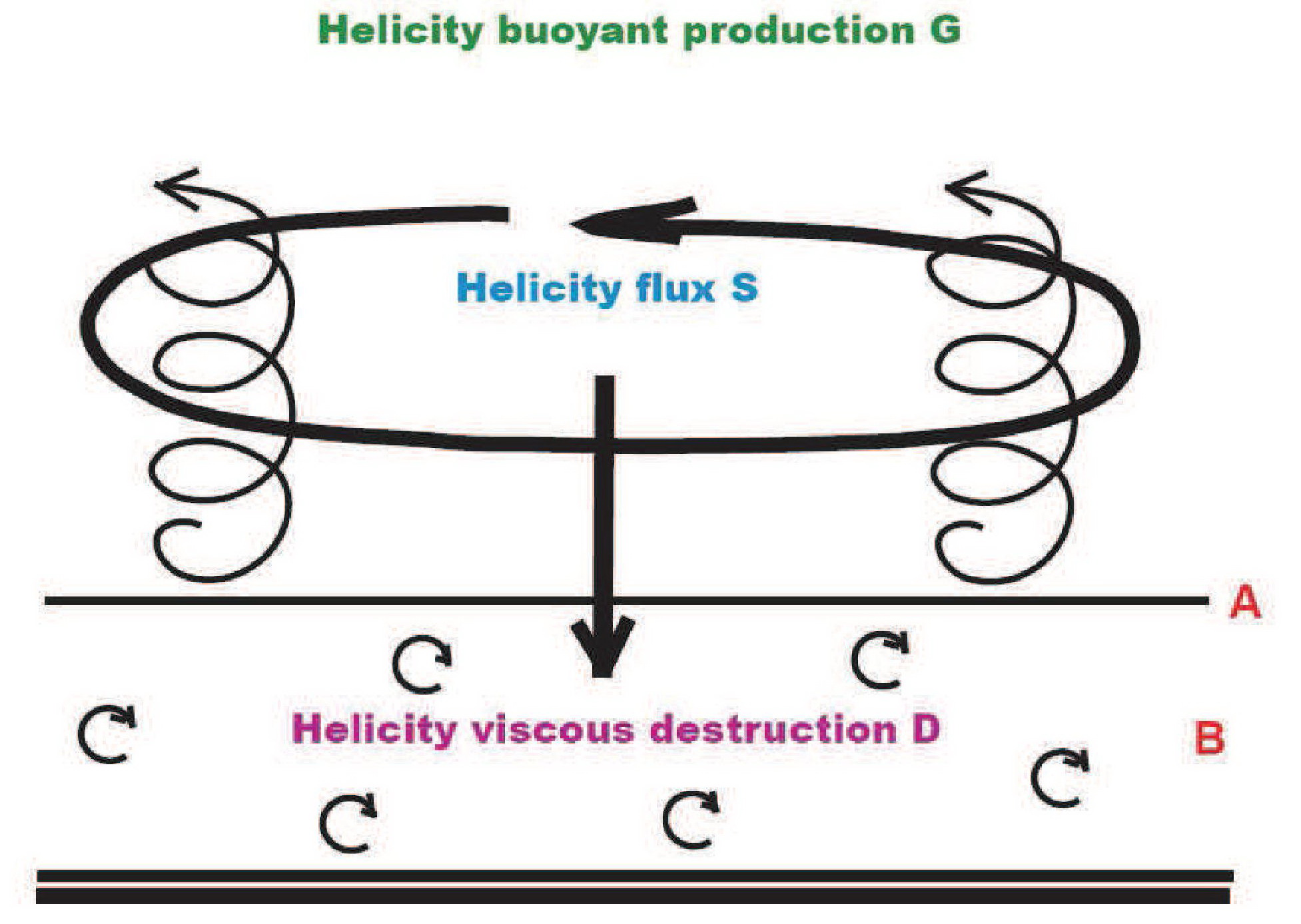
Figure 1.1: A schematic of helicity balance in intense atmospheric vortices. The vortex flow is outlined by a thick curved arrow. Helicity flux $\displaystyle S$ is shown by a downward pointing arrow. Small-scale turbulence within the boundary layer is presented by small curved arrows. A thick double horizontal line shows the Earth’s surface.

Kurgansky (2008) proposed using vertical helical flux in small and mesoscale vortices as a measure of their intensity. For a steady axisymmetric vortex in the polar cylindrical coordinates under the neglect of the small radial velocity component $\displaystyle u$, this downward directed helicity flux through the upper level $\displaystyle A$ of the turbulent boundary layer reads Kurgansky (2017)

$$S=\iint\limits_{A}\left(2v^{2}-w^{2}\right)\,\omega_{z}{\rm d}\sigma.$$ (1.6)

Here, $\displaystyle v$ is the azimuthal velocity component, $\displaystyle w$ the vertical velocity component, $\displaystyle\omega_{z}$ the vertical vorticity, and $\displaystyle{\rm d}\sigma$ the surface area element; it has been used that $\displaystyle rv\left.w^{2}\right|_{r=0}^{r=\infty}=0$. Here we come to an important point. As already follows from Moffatt (1969) and confirmed by the analysis of (1.4), the helicity flux has both the advective (velocity-driven) and non-advective (along the vortex lines) component. As a rule, the latter component, for example in intense atmospheric vortices, significantly exceeds the former, as it is accounted for in (1.6); see also Kurgansky (2017). The effect of Earth rotation with the angular velocity $\displaystyle{\bm{\Omega}}$ has been neglected. If needed, its account would result in appearance of the additional term $\displaystyle\iint\limits_{A}\left(2{\bm{\Omega}}\cdot\mathbf{k}\right)\,v^{2}{\rm d}\sigma$ on the right side of (1.6), where $\displaystyle\mathbf{k}$ is the unit vertical vector.

In atmospheric vortices of small and mesoscales, as a rule, $\displaystyle u<\left(\ll\right)w<\left(\ll\right)v$. For example, based on direct measurements from aircraft in waterspouts in Leverson et al. (1977), the characteristic values are as follows: $\displaystyle v=25\,{\rm m}\,{\rm s}^{-1}$, $\displaystyle w=8\,{\rm m}\,{\rm s}^{-1}$ and $\displaystyle u=1\,{\rm m}\,{\rm s}^{-1}$. Therefore, instead of (1.6), the approximate formula can be used, see Kurgansky (2008, 2017)

$$S\cong\iint\limits_{A}2v^{2}\omega_{z}{\rm d}\sigma,$$ (1.7)

or alternatively, $\displaystyle S\cong\left({8\pi/3}\right)\int\limits_{0}^{\infty}v^{3}{\rm d}r$, if only $\displaystyle v^{3}r\to 0$ with $\displaystyle r\to\infty$, where $\displaystyle r$ is the radial coordinate. Glebova et al. (2009) applied the method of helicity fluxes to the Man-Yi (2007) and Wilma (2005) tropical cyclones and Farahani et al. (2017) did it for the tropical storm Gonu (2007).

For the combined Rankine vortex with the uniform vertical flow inside the vortex core and under neglect of the Coriolis force, the vertical helicity flux in a vortex is estimated by the value $\displaystyle S=2\pi V\left(V^{2}-W^{2}\right)R$, see (1.6), where $\displaystyle V$ is the maximum azimuthal velocity, $\displaystyle W$ the vertical velocity and $\displaystyle R$ the vortex core radius, and if $\displaystyle V\gg W$, then $\displaystyle{\rm S}\approx 2\pi V^{3}R$; see (1.7) and Kurgansky (2013b). The natural time scale for vortices is the time of their complete revolution around the axis $\displaystyle{2\pi R/V}$. For example, the use of data in Lorenz (2013) allows us to conclude that dry-convective small-scale dust-devil vortices, regardless of their size, have a life-duration on average about 60 revolutions. Simply, in large vortices this revolution takes a longer time, therefore, in absolute units of time, they live longer. The ratio $\displaystyle{{\cal H}/S}$, where $\displaystyle{\cal H}=4\pi VWRH$ is the total helicity of the vortex flow and $\displaystyle H$ is the height of the vortex (see above), determines the characteristic time of the helicity transformation (helicity metabolism) in the vortex flow. For dust devils, this time is short and equates to only few complete revolutions of the vortex around its axis. If we put $\displaystyle{H/R}=10$ (Lorenz, 2013; Jackson, 2020) and accept that $\displaystyle{V/W}=3$, then the estimate shows that the time of the complete renewal of helicity in the vortex is $\displaystyle\sim 6$ complete revolutions of the dust devil around its axis, i.e. during a typical dust-devil vortex lifetime, the vortex helicity has time to be completely renewed about 10 times. From this perspective, one can say that helicity is a kind of constantly renewing corset (frame) that energy fills in. The claim about a shorter helicity destruction time, compared to energy dissipation, is generally consistent with the conclusions of Levshin and Chkhetiani (2013), who showed that helicity in homogeneous turbulence decays faster than energy. The same is true for the large-scale extratropical atmospheric motions. The rate of destruction of the helicity within the Ekman boundary layer is equal to the downward flux of helicity from the free atmosphere. This flux is determined (per unit area of the Earth’s surface) by the product of the Coriolis parameter and the square of the geostrophic wind speed in the free atmosphere (Kurgansky, 1989, 1993, 2002); also Deusebio and Lindborg (2014). Therefore, the helicity transformation time in large-scale extratropical atmospheric processes is given by the reciprocal of the Coriolis parameter ($\displaystyle\sim 10^{4}\,{\rm s}$) and by a factor of ten it is less than the characteristic duration of large-scale cyclones and anticyclones.

Until now, the main emphasis has been on observations of helicity but not on its dynamics. The above arguments about helicity balance and its “metabolism” apply to a quasi-steady mature stage of atmospheric vortices. The issue of helicity generation (genesis) is more complex and non-trivial. Helicity is conserved and therefore cannot be generated in barotropic flows of inviscid fluids in the presence of potential forces (Moreau, 1961; Moffatt, 1969). So, the genesis of helicity requires the violation of the above conditions, that is, it requires the joint action of atmospheric baroclinicity, which often takes the form of vertical convection leading to vertical flows, and the general rotation of the flow system, either directly or indirectly related to the Earth’s rotation. In the latter case the sense of Earth’s rotation is “transmitted” through the sequence of emerging circulation systems of progressively decreasing spatial scale (cold atmospheric fronts, mesocyclones, etc.), in which tornadoes are embedded, almost all them (with rare exceptions) being cyclonic vortices. There are indications that surface friction may also contribute to the genesis of helicity. The small-scale dynamics of helicity is important for tornadoes. In particular, these are Hasimoto solitons (Hasimoto, 1972) propagating along strong vortex filaments (thin tornadoes) and Aref and Flinchem (1984) have provided photographs of a tornado near Braman, Oklahoma (11 May 1978) showing localized large-amplitude helical twist in the vortex core (a “soliton”). Holm and Stechmann (2004) showed that the nonlinear Schrödinger equation in Hasimoto (1972) is replaced by the integrable complex modified Korteweg–de Vries equation having soliton solutions, when the Hamiltonian in the underlying theory is not the kinetic energy but helicity. The classical case of kinetic energy and the case of helicity discussed in Holm and Stechmann (2004) exhaust all Hamiltonians that have fluid dynamical significance (ibid).

1.4 Helical turbulence in the Earth’s atmosphere

Moving from the discussion of general principles in Section 1.2 to a more detailed consideration of helical turbulence, particularly in the Earth’s atmosphere, we first mention successful attempts to numerically reproduce cascades of energy and helicity directed differently, but taking into account the general rotation of the fluid (Mininni and Pouquet, 2010a, b; Pouquet and Mininni, 2010). However, Biferale et al. (2012, 2013) and Sahoo et al. (2017) showed that without general rotation but by allowing interactions between helical modes of the same sign (homochiral modes), the inverse cascade of energy is possible as in the two-dimensional turbulence. Gledzer and Chkhetiani (2015); Chkhetiani and Gledzer (2017), also using the turbulent cascade model with conservation of helicity (Gledzer, 1973), show that to reproduce the inverse energy cascade from small-scale disturbances, a certain level of “helical noise” is necessary in large-scale modes, which is generated by external forcing. These conclusions are also supported by an analysis of second-order moments in the quasi-normal approximation. Similar results were also obtained in Stepanov et al. (2015). Another line of research uses the formulation of three-dimensional turbulent fields in terms of helical modes introduced in Knorr et al. (1990) and Waleffe (1992), which was applied in Rathmann and Ditlevsen (2017) to investigate some details in joined energy and helicity cascades.

An important research line is related to direct numerical simulation (DNS) studies on helicity which are only briefly described here. In particular, they include DNS studies on turbulence decay by Holm and Kerr (2002). Their diagnostics showed that the turbulence initial value problem evolves through an early stage, with still negligible dissipation, when vortex sheets form from smooth initial conditions and then coil into helical vortex tubes. Once the helical vortex tubes have formed, viscous dissipation grows rapidly in the DNS and the energy spectrum gradually approaches the classical “-5/3” law characteristic of a turbulent energy cascade, but before is achieved, the energy spectrum remains steeper than “-5/3”; see Fig. 6 in Holm and Kerr (2002). Once a clear “-5/3” spectrum appears, the energy decay becomes self-similar. The numerical study of the joint cascade of energy and helicity by three-dimensional DNS was carried out by Chen et al. (2003) and verified their theoretical conclusions that the Kolmogorov microscale of turbulence is the minimum scale of helical motions for a joint cascade of energy and helicity (see also below). DNS studies of helical turbulent flows continue and are actively developing today. It is beyond the scope of this review to list all relevant papers; see, for example, a recent article by Biferale et al. (2019).

Chkhetiani (1996) obtained an important relation between the two-point triple correlation of the velocity and the rate of helicity transfer over the spectrum and, therefore, of its viscous destruction at small scales. Later it was called the “2/15 law” for helicity, which is dual to the “4/5 law” of A.N. Kolmogorov for the velocity field in three-dimensional non-helical turbulence, and is similar to the “4/3 law” of A.M. Yaglom for a passive scalar (Chkhetiani, 2008); see also (Golitsyn, 2012, § 6.1.6). The “2/15 law” allows to obtain the spectra of helicity, both the “-5/3 law”, when the helicity behaves as a passive scalar, and the more hypothetical “-4/3 law”, when the helicity cascade is decisive.

More in detail, two cases of the turbulent cascade of helicity are possible. The first case is the joint cascade of energy and helicity towards small scales. The spectral slope of helicity coincides in this case with the slope of the energy spectrum and is equal to $\displaystyle-$5/3

$$\hat{E}(k)=c_{E}\varepsilon^{2/3}k^{-5/3},\quad\hat{H}(k)=c_{H}\eta\,\varepsilon^{-1/3}k^{-5/3}.$$ (1.8)

The second case is the direct cascade of helicity and inverse cascade of energy (Brissaud et al. 1973)

$$\hat{E}(k)=c_{E}^{*}\eta^{2/3}k^{-7/3},\hat{H}(k)=c_{H}^{*}\eta^{2/3}k^{-4/3}.$$ (1.9)

Here $\displaystyle\hat{E}(k)$ and $\displaystyle\hat{H}(k)$ are the spectral densities of energy $\displaystyle{\cal E}={\frac{1}{2}}\left\langle\mathbf{v}^{2}\right\rangle$ and helicity $\displaystyle{\cal H}=\left\langle\mathbf{v}\cdot{\bm{\omega}}\right\rangle$ , respectively; $\displaystyle\varepsilon=\nu\langle(\bm{\nabla}\times\mathbf{v})^{2}\rangle$ is the specific kinetic energy dissipation rate and $\displaystyle\eta=\nu\langle{\bm{\omega}}\cdot\bm{\nabla}\times{\bm{\omega}}\rangle$ is the time rate of helicity viscous destruction; $\displaystyle k$ is the wavenumber, $\displaystyle\nu$ the kinematic viscosity and angular brackets denote ensemble averaging. Additionally, we note that in this case, the Obukhov–Corrsin spectrum of temperature fluctuations (passive scalar) and the co-spectrum of the temperature $\displaystyle T$ and vertical velocity $\displaystyle U_{3}$ fluctuations will also have different slopes (Moiseev and Chkhetiani, 1996)

$$\hat{E}_{TT}(k)\sim N\eta^{-1/3}k^{-4/3},\hat{E}_{TU_{3}}(k)\sim N\eta^{-1/6}k^{-7/6}$$ (1.10)

compared with the $\displaystyle-$5/3 in the usual case. Here, $\displaystyle N=\chi\left\langle(\nabla T)^{2}\right\rangle$ is the average rate of dissipation of temperature inhomogeneities. Let us also note that the analogue of the Bolgiano–Obukhov scale $\displaystyle L_{*}=\eta^{-5}N^{3}(g\beta)^{6}$ arises in comparison with $\displaystyle L_{BO}=\varepsilon^{5/4}(g\beta)^{-3/2}N^{-3/4}$, where $\displaystyle\beta={1/T_{0}}$ with $\displaystyle T_{0}$ as the constant reference temperature. For a long time, the existence of the helical cascade (1.9) was considered hypothetical. In particular, the conditions for the realization of inverse energy cascades were considered difficult to fulfill in real conditions, although, certain spectra observed in the atmosphere and in laboratory experiments had spectral slopes quite close to those in (1.9) (Chkhetiani et al., 2006). It is only relatively recently that such regimes began to be reproduced in numerical experiments using helicity pumping at different scales (Biferale et al., 2012, 2013; Sahoo et al., 2017; Gledzer and Chkhetiani, 2015).

The presence of helicity in turbulence manifests itself in the appearance in the tensor of two-point triple correlations of the velocity field those components, which are identically equal to zero in its absence (Chkhetiani et al. 1996), and it holds that

$$\langle\delta\mathbf{v}_{l}(x|r)\cdot[\mathbf{v}_{t}(x+r)\times\mathbf{v}_{t}(x)]\rangle=\frac{2}{15}\eta r^{2}.$$ (1.11)

The indicated dependence (the so-called 2/15 law) is similar to the Kolmogorov 4/5 law for longitudinal velocity correlations (cf. Monin and Yaglom, 1971, 1975)

$$\langle\left(\delta\mathbf{v}_{l}(x|r)\right)^{3}\rangle=-\frac{4}{5}\varepsilon r.$$ (1.12)

and is the exact result following from the Navier–Stokes equations. Here, the velocity field is divided into longitudinal and transverse components respective to the vector $\displaystyle r$ connecting the observation points, $\displaystyle\mathbf{v}_{l}=\left(\mathbf{v}\mathbf{r}\right)\mathbf{r}/r^{2}$, $\displaystyle\mathbf{v}_{t}=\mathbf{v}-\mathbf{v}_{l}$, $\displaystyle\delta\mathbf{v}_{l}\left(\mathbf{x}|\mathbf{r}\right)=\left(v_{l}(\mathbf{x}+\mathbf{r})-v_{l}(\mathbf{x})\right)\mathbf{r}/r$. Denoting $\displaystyle r_{i}=r\delta_{ix}$ we obtain for the two-point triple tensor of velocity and vorticity correlations the following representation (Chkhetiani, 2008)

$$T_{i,j,k}=\left\langle v_{i}\left(\mathbf{x}\right)v_{j}\left(\mathbf{x}\right)\omega_{k}\left(\mathbf{x}+\mathbf{r}\right)\right\rangle=\frac{\eta r}{15}\delta_{ij}\delta_{kx}-\frac{\eta r}{10}\left(\delta_{ix}\delta_{jk}+\delta_{ik}\delta_{jx}\right).$$ (1.13)

The understanding of the presence of helicity in atmospheric turbulence came later. Thus, in the work of Novikov (1972), where the statistical properties of the vorticity flux tensor

$$\langle v_{i}\omega_{j}\rangle=\frac{\varepsilon_{ikl}}{4\pi}\int\limits_{V}\frac{r_{l}}{r^{3}}\langle\omega_{k}(\mathbf{x}^{\prime})\omega_{j}(\mathbf{x})\rangle{\rm d}^{3}\mathbf{x}^{\prime},$$ (1.14)

were discussed, the diagonal elements of this tensor, which are directly related to helicity, were not considered. According to Novikov (1972), only four non-diagonal elements of (1.14), $\displaystyle\left\langle u^{\prime}\omega^{\prime}_{2}\right\rangle$, $\displaystyle\left\langle v^{\prime}\omega^{\prime}_{1}\right\rangle$, $\displaystyle\left\langle w^{\prime}\omega^{\prime}_{1}\right\rangle$ and $\displaystyle\left\langle u^{\prime}\omega^{\prime}_{3}\right\rangle$, where $\displaystyle\mathbf{v}=\left(u,v,w\right)$, should be different from zero in the atmospheric boundary layer (ABL) turbulence. The first measurements of the covariance between the velocity and vorticity components and the corresponding co-spectra and spectra, were carried out at heights of 1.2 and 5 m at the Tsimlyansk test site of the Institute of Atmospheric Physics, Russian Academy of Sciences (Koprov et al., 1988) using an acoustic circulation-meter (the so-called, “circulimeter”) first designed and manufactured by Bovsheverov et al. (1971). The observed differences from zero of the covariance, associated with the circulation in the vertical plane parallel to the mean flow directed along the $\displaystyle x$-axis and corresponding to $\displaystyle\left\langle v^{\prime}\omega^{\prime}_{2}\right\rangle$, were clearly not consistent with the conclusions of Novikov (1972). In addition, a strong correlation was found between the velocity circulation and the temperature field.

To measure helicity, measurements of all three components of the velocity and vorticity are required. Vorticity measurement techniques can be conditionally divided into direct and indirect ones. Direct measurements with hot-wire arrays were carried out in Wyngaard (1969); Antonia et al. (1988); Vukoslavcevic and Wallace (1996) and Kholmyansky et al. (2001). Providing the ability to carry out measurements on scales close to the dissipation range, this technique poorly matches to the conditions of a real ABL. Indirect methods are associated with the measurement of circulation along a certain contour and, accordingly, the determination of the average vorticity over the area encircled by the contour, based on the application of the Stokes theorem (Bovsheverov et al., 1971; Koprov et al., 1988, 1994, 2005). Ideologically close techniques for measuring atmospheric circulation were also proposed in Jordan (1980); Ohtou et al. (1983) and Mitsuta and Asai (1984). Such techniques were often used to determine the characteristics of oceanic turbulence (Rossby, 1975; Gaynor et al., 1977; Thwaites et al., 1995; Sanford et al., 1999). The procedure for calculating the velocity circulation was discussed in detail by Longuet-Higgins (1982). In Koprov et al. (1994, 2005), synchronized measurements of velocity and circulation were made using one- and two-component acoustic “circulimeters” with a contour diameter of 1 m together with an acoustic anemometer. All three sensors were placed on top of a 46-m high mast, with the anemometer in the center, and the “circulimeters” on both sides of it at a distance of 0.8 m. The spectra of helicity components with a slope close to –5/3 were observed (Fig. 1.2); see Koprov et al. (2005). An integral estimate of helicity from the observed spectrum gives the values of 0.02–0.03 ms^-2. For the components of the two-point tensor triple product of the velocity and vorticity components $\displaystyle\left\langle v_{i}\left(\mathbf{x}\right)v_{j}\left(\mathbf{x}\right)\omega_{k}\left(\mathbf{x}+\mathbf{r}\right)\right\rangle$ in the same frequency range as for the helicity components, the spectrum slope close to -1 is observed (Fig. 1.3).

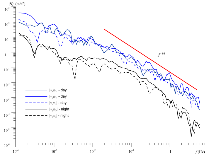
Figure 1.2: Frequency spectra of the contributions to helicity calculated based on the 2-hour records: the nighttime of 11.09.14 with the onset at 22:17 local time and the daytime of 12.09.14 with the onset at 13:41 local time (Koprov et al., 2005).

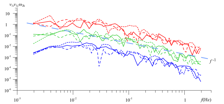
Figure 1.3: The triple correlation frequency spectra calculated from the 2-hour records of the velocity and circulation components from 28.08.04 with the onset at 11:38 local time (red line), at 16:41 local time (green line), and from 11.09.04 with the onset at 22:17 local time (blue line). The solid line shows the $\displaystyle\left\langle v_{y}v_{z}\omega_{y}\right\rangle$ spectrum, the long dashed line – $\displaystyle\left\langle v_{x}v_{z}\omega_{y}\right\rangle$ spectrum, and the short dashed line – $\displaystyle\left\langle v_{x}v_{y}\omega_{y}\right\rangle$ spectrum.

In a field campaign in Tsimlyansk, Russia in August 2012, Koprov et al. (2015) use four three-component acoustic anemometers in the vertices of a rectangular tetrahedron with the side of 5 m and its base at 5.5 m above the ground (Fig. 1.4). Two different methods of calculating helicity were applied. First, the velocity circulations along the contours encircling the tetrahedron faces were calculated and then the Stokes theorem was applied to calculate the corresponding average vorticities, $\displaystyle\omega_{x}$, $\displaystyle\omega_{y}$ and $\displaystyle\omega_{z}$, and thus the helicity. Second, an alternative finite-difference method for approximating, $\displaystyle\omega_{x}$, $\displaystyle\omega_{y}$ and $\displaystyle\omega_{z}$ in point A (see Fig. 1.5)was applied to calculate helicity, see (1.15),

$$H_{A}=u_{A}\left(\omega_{x}\right)_{A}+v_{A}\left(\omega_{y}\right)_{A}+w_{A}\left(\omega_{z}\right)_{A}$$

$$\approx\frac{w_{A}u_{B}-u_{A}w_{B}}{L_{AB}}+\frac{v_{A}u_{D}-u_{A}v_{D}}{L_{AD}}+\frac{w_{A}v_{C}-v_{A}w_{C}}{L_{AC}}.$$ (1.15)

The three components $\displaystyle\left(u,v,w\right)$ of velocity are measured in points A, B, C and D; $\displaystyle L_{AB}$, $\displaystyle L_{AD}$ and $\displaystyle L_{AC}$ are the lengths of the tetrahedron edges, see Fig. 1.5. Both methods give similar results.

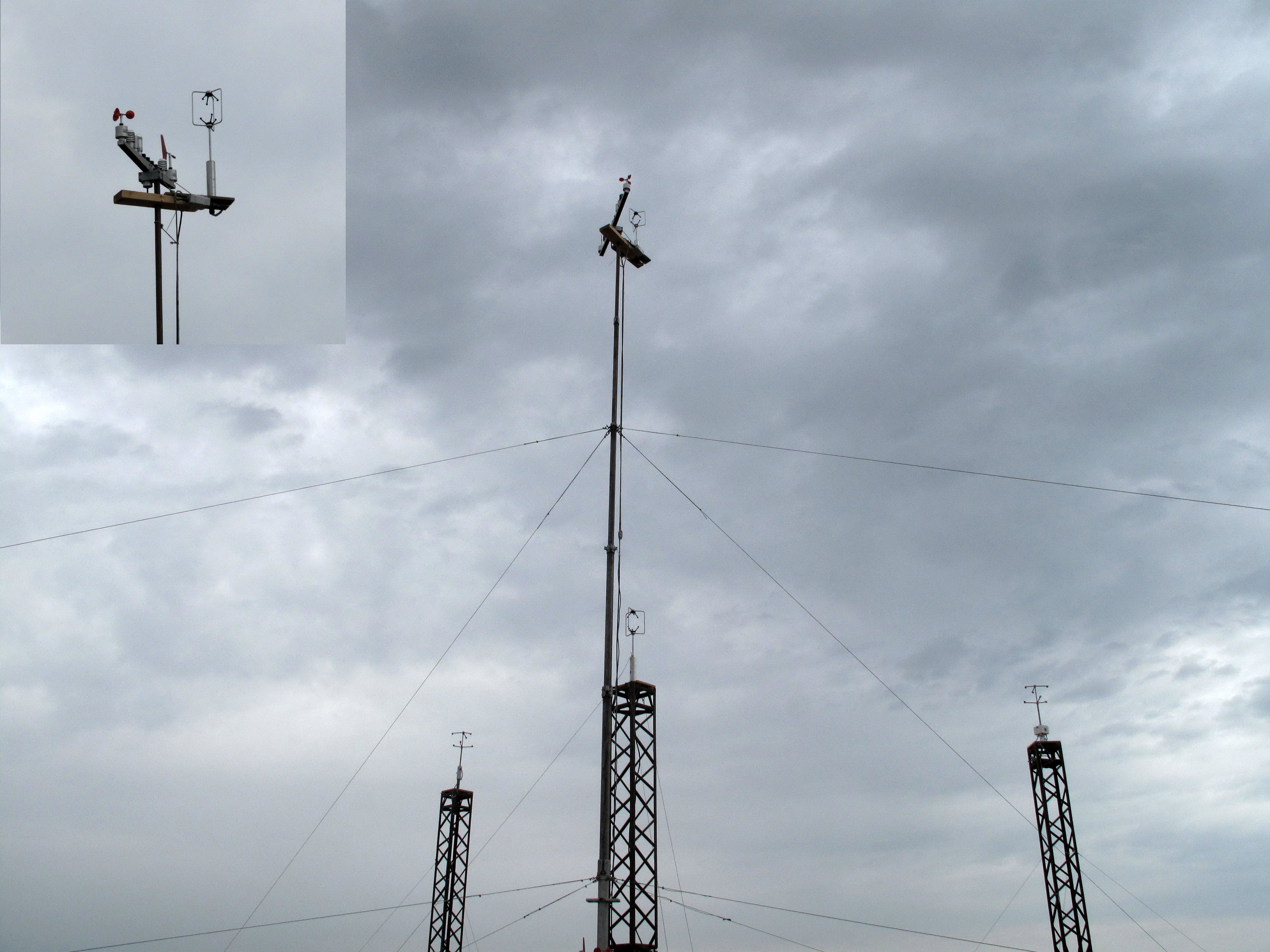
Figure 1.4: Photo of the tetrahedron composed of four sonic anemometers to measure helicity in Koprov et al. (2015); see also Chkhetiani et al. (2018). An enlarged image of the uppermost anemometer at 10-m height assembled with a cup anemometer and a windvane (temperature, pressure and humidity sensors) is in the upper left corner. (Photo copyright O. Chkhetiani)

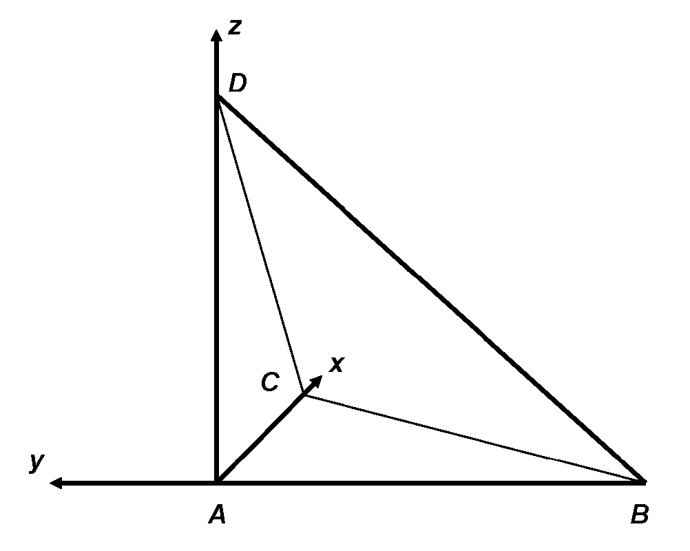
Figure 1.5: Schematic of the rectangular tetrahedron ABCD used for helicity measurements; the (x, y) axes are directed north and west, respectively. Three anemometers are positioned at the vertices of a rectangular isosceles triangle ABC with sides AB and AC equal to 5 m. The fourth anemometer at point D is located 5 m higher, just above poimnt A; see also Chkhetiani et al. (2018).

Turbulent helicity measured values are shown in Table 1.2. Primes denote deviations from the values, obtained by running mean averaging with a 30-seconds rectangular window; $\displaystyle\theta^{\prime}$ is the temperature fluctuation. Hereafter, an overbar denotes averaging over the entire measurement session. More details are given in Chkhetiani et al. (2018).

Table 1.2: The values of co-variances obtained experimentally in Koprov et al. (2015), see also Chkhetiani et al. (2018). The $\displaystyle x$-axis is directed north, the $\displaystyle y$-axis west, and the $\displaystyle z$-axis up. Values in the middle row correspond to the measurement session from 12:38 to 16:30 local time (UTC + 3 h) on 8 August 2012. The numbers in the lower row correspond to the measurement session from 22:46 to 00:34 local time, the end of the session on 9 August 2012.

	$\displaystyle\overline{u^{\prime}\omega^{\prime}_{x}}$, ms-2	$\displaystyle\overline{v^{\prime}\omega^{\prime}_{y}}$, ms-2	$\displaystyle\overline{w^{\prime}\omega^{\prime}_{z}}$, ms-2	$\displaystyle\overline{w^{\prime}\theta^{\prime}}$, mKs-1	$\displaystyle\overline{\omega^{\prime}_{z}\theta^{\prime}}$, Ks-1
Day	–0.0170	–0.0276	0.0143	0.1545	0.0456
Night	–0.0138	–0.0010	0.0085	–0.0172	–0.0123

We emphasize that for the negative mean helicity the instantaneous helicity values can be of any sign and the negative ones dominate only in a statistical sense, and the corresponding standard deviation is significantly higher than the mean value, see Fig. 1.6.

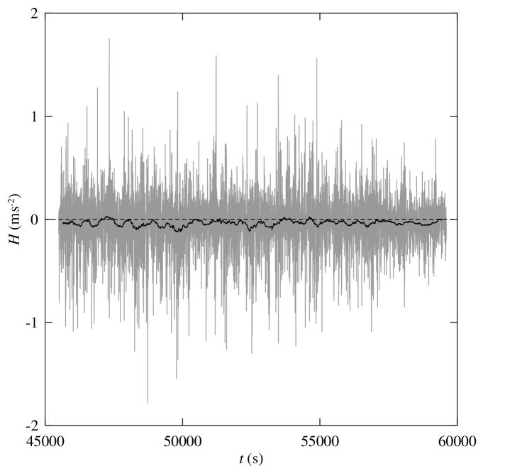
Figure 1.6: Turbulent helicity $\displaystyle H^{\prime}$ values (in ms^-2) measured during the day in Koprov et al. (2015) and averaged over 1 sec (thin grey line); see Table 1.2 and Chkhetiani et al. (2018). The abscissa shows the elapsed time (in seconds) since the beginning of the day. A solid line shows 5-min averages of $\displaystyle H^{\prime}$.

Figure Fig. 1.7 shows the histogram of turbulent helicity $\displaystyle H^{\prime}$ values presented Fig. 1.6. The measurement session lasted 14,113 seconds, therefore dividing the $\displaystyle N$ values in Fig. 1.7 by 14,113 we infer the probability density function of $\displaystyle H^{\prime}$ values, which can be compared with Fig. 7 in Deusebio and Lindborg (2014) for an idealized Ekman layer in the Northern Hemisphere, where, in contrast, positive turbulent helicity values dominate.

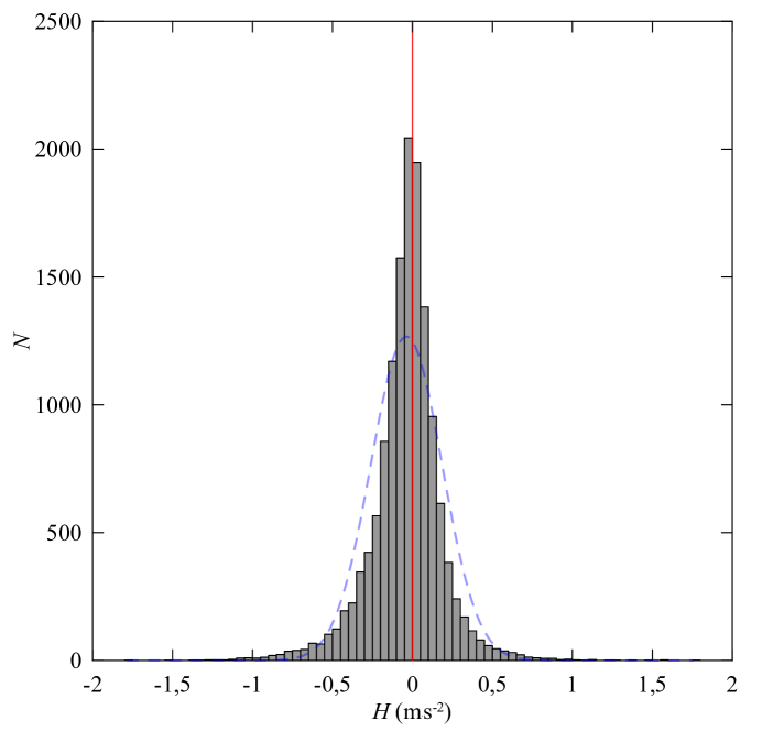
Figure 1.7: Histogram of instantaneous turbulent helicity values measured in Tsimlyansk, southern Russia on 8 August 2012 at 12:38$\displaystyle-$16:30 local time (Koprov et al. (2015); see the text for more details). On the horizontal axis the turbulent helicity values (in ms^-2) are shown; the width of each bin equals 0.05 ms^-2. On the vertical axis, the numbers show the number N of helicity values falling within the corresponding bin. The sum of all N values equals 14,113 (see the text). A vertical red line shows zero helicity values H $\displaystyle=$ $\displaystyle 0$. For comparison, a Gaussian distribution that has the same dispersion is shown by a blue dashed line.

We now proceed to compare the experimental results by Koprov et al. (2015) with theoretical estimates following the idealized conceptual scheme by Deusebio and Lindborg (2014). More details are given in Chkhetiani et al. (2018). Here, only the main stages of reasoning are described. In the Northern Hemisphere, positive helicity is injected from the free atmosphere into the Ekman boundary layer with the time rate $\displaystyle f\mathbf{u}_{g}^{2}$, where $\displaystyle\mathbf{u}_{g}$ is the vector of geostrophic wind. Furthermore, helicity is cascaded as an effective passive scalar quantity towards smaller scales to be finally destroyed by viscosity. Then it follows that the helicity destruction rate in the lower part of the Ekman boundary layer reads

$$\eta=2f\mathbf{u}_{g}^{2}/h_{E},$$ (1.16)

where $\displaystyle h_{E}=\sqrt{2K/f}$ is the Ekman boundary layer thickness, $\displaystyle K$ is the small-scale eddy viscosity, $\displaystyle f$ the Coriolis parameter, and the factor ”two” is derived from more detailed considerations of helicity and superhelicity of the classical Ekman spiral solution in Kurgansky (1989): see more in Chkhetiani et al. (2018). Turbulent helicity $\displaystyle H^{\prime}\equiv\overline{{\mathbf{u}^{\prime}}\cdot{\bm{\omega}^{\prime}}}=H^{\prime}\left(l\right)$ on the given spatial scale $\displaystyle l$ that belongs to an inertial interval can be estimated from Brissaud et al. (1973),

$$H^{t}\left(l\right)=C_{H}\eta\,\varepsilon^{{-1/3}}l^{{2/3}},$$ (1.17)

which corresponds to the joint cascade of energy and helicity to small scales to cf. (1.9); see also Chen et al. (2003). In (1.17), $\displaystyle C_{H}$ has been estimated either as 2.3 (André and Lesieur, 1977) or 2.5 (Avinash et al., 2006). Taking $\displaystyle h_{E}=400\,{\rm m}$, $\displaystyle f=10^{-4}{\rm s}^{-1}$, $\displaystyle\left|u_{g}\right|=10\,\,{\rm m}\,{\rm s}^{-1}$, $\displaystyle\varepsilon=10^{-3}\,{\rm m}^{2}{\rm s}^{-3}$, $\displaystyle C_{H}=2.4$, and $\displaystyle l\,=10\,{\rm m}$, cf. Koprov et al. (2005), we obtain $\displaystyle H^{t}\approx 5.5\times 10^{-3}\,{\rm m}\,{\rm s}^{-2}$, that is, several times smaller than the daytime $\displaystyle H^{t}$ values measured in Koprov et al. (2005).

In fact, a lower estimate was for $\displaystyle H^{t}$, which ignores other possible sources of turbulent helicity in the bottom part of the planetary boundary layer. Chkhetiani et al. (2018) discuss these and other possible complicating factors. The analysis of meteorological conditions during the field campaign in Koprov et al. (2015) suggests that the joint action of the Ekman spiral flow and the sea-breeze circulation explains the resulting negative sign of $\displaystyle H^{\prime}$ and its magnitude, see Table 1.2 and Chkhetiani et al. (2018). This hypothesis was tested using the balance model of $\displaystyle H^{\prime}$ in the planetary boundary layer (Chkhetiani et al., 2018).

It is also mentioned in Chkhetiani et al. (2018) that the scale $\displaystyle\lambda_{D}\sim\varepsilon^{{2/7}}\nu^{{3/7}}\left({2fu_{g}^{2}/h_{E}}\right)^{-{3/7}}$ obtained by equating (1.16) and $\displaystyle\eta=2\nu\overline{{\bm{\omega}}^{\prime}\cdot\nabla\times{\bm{\omega}}^{\prime}}$ corresponds to the Ditlevsen scale (Ditlevsen and Giuliani (2001a, b); see also Ditlevsen (2010)). Here, $\displaystyle\nu$ is the air molecular viscosity. For the parameter values pertinent to the measurement site in Tsymlyansk $\displaystyle\lambda_{D}\sim 1.1\times 10^{-1}{\rm m}$ is two orders of magnitude greater than the Kolmogorov microscale of turbulence, which is the minimum scale of helical motions for a joint cascade of energy and helicity (Chen et al. (2003); see also, Briard and Gomez (2017)).

For a thermally stratified boundary layer the turbulent helicity reads (Chkhetiani et al., 2018)

$$H^{t}=2K\tau\left(\frac{d^{2}U}{dz^{2}}\frac{dV}{dz}-\frac{d^{2}V}{dz^{2}}\frac{dU}{dz}\right)+f\frac{d\,\overline{w^{\prime 2}}}{dz}\,\tau+2\alpha g\overline{\omega^{\prime}_{z}\theta^{\prime}}\,\tau.$$ (1.18)

where $\displaystyle\alpha>0$ is the coefficient of thermal expansion of air and $\displaystyle\tau$ the turbulent relaxation time. There are three different terms in the expression for $\displaystyle H^{\prime}$. The first term corresponds mainly to $\displaystyle\overline{u^{\prime}\omega^{\prime}_{x}}+\overline{v^{\prime}\omega^{\prime}_{y}}$ and an expression in parentheses represents the superhelicity $\displaystyle S$ of the mean flow. In the absence of the other two terms in (1.18), this term denotes $\displaystyle H^{\prime}<0$ for $\displaystyle S<0$. The second term, generally positive in the Northern Hemisphere is two or three orders of magnitude smaller than the first term. The third term is due to thermal stratification and corresponds to the three contributions to helicity, including $\displaystyle\overline{w^{\prime}\omega^{\prime}_{z}}$. As the data in Table 1.2 show, it is positive during the day and negative at night, respectively.

For the third term in (1.18) we have in a steady statistically equilibrium turbulent regime

$$\tau^{-1}\overline{\omega^{\prime}_{z}\theta^{\prime}}\approx\overline{w^{\prime}\left(\overline{{\bm{\omega}}}\cdot\nabla\theta^{\prime}\right)}+\overline{w^{\prime}\left({\bm{\omega}}^{\prime}\cdot\nabla\theta^{\prime}\right)}.$$ (1.19)

It should be noted that the right-hand side of (1.19) is nothing but a mutual correlation of the vorticity fluctuations and the turbulent Ertel potential vorticity. In Fig. 1.8 we show the time dependence of two fluctuating quantities, $\displaystyle P\equiv\omega^{\prime}_{z}\theta^{\prime}$ and $\displaystyle Q\equiv\left(w^{\prime}\left(\overline{{\bm{\omega}}}\cdot\nabla\theta^{\prime}\right)+w^{\prime}\left({\bm{\omega}}^{\prime}\cdot\nabla\theta^{\prime}\right)\right)$, for the daytime measurements in Koprov et al. (2015), see Table 1.2. A 10-min averaging is used to plot $\displaystyle P$ and $\displaystyle Q$, and the correlation between these quantities is evident in Fig. 1.8. Analogous results are obtained for the nighttime measurements in Koprov et al. (2015).

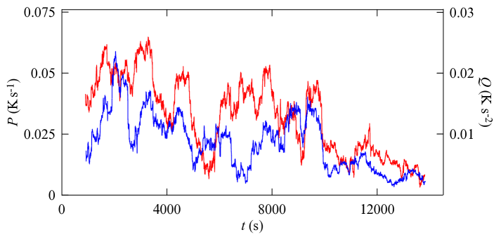
Figure 1.8: Time dependence of $\displaystyle P$ (in Ks^-1, red line) and $\displaystyle Q$ (in Ks^-2, blue line) values, for the daytime measurements in Koprov et al. (2015), see also Table 1.2 and the text for details. On the horizontal axis, zero corresponds to 12:48 local time (Chkhetiani et al., 2018).

In 2014, measurements were carried out using a similar scheme with a basic setup scale of 0.7 m at heights of 3.5, 13.1, and 25 meters (Koprov et al., 2018). Differences from zero of all three diagonal elements of the vorticity flux tensor, the correlation of the vorticity with the temperature field, and spectral dependences for helicity were found, close to those following from the concept of the constancy of the helicity flux towards small scales in the inertial interval.

1.5 Concluding remarks and outlook

The role and significance of the concept of helicity in atmospheric physics will be fully appreciated in the future. Among other things, this Chapter discusses the relationship between the concepts of helicity and potential vorticity, which is especially non-trivial in a compressible fluid. There is a certain complementarity of the concepts of potential vorticity and helicity. The first of them, historically at least, was mainly demanded for the “clarification” of the principles of the dynamics of large-scale processes. At the same time, the concept of helicity for such motions is not very significant (meaningful). The situation changes as the transition to meso- and then small-scale atmospheric motions occurs. It is not to say that the concept of potential vorticity is completely losing its meaning. In a sense, it becomes less constructive, since the “invertibility principle” (Hoskins et al., 1985), that is, the possibility of restoring all other (balanced) hydrodynamic fields from the known field of a potential vorticity, gradually loses its applicability. For large-scale motions, this possibility is guaranteed by the quasi-geostrophic theory and its improvements. For meso- and small-scale motions, considerations of symmetry (axial, etc.) are indispensable. At the same time, the helicity concept acquires more weight and its alignment occurs in the conceptual sense with the potential vorticity, which makes its connection with the latter more important.

As for the study of helical turbulence, which is the central theme of the second part of this Chapter, it must be said with certainty that it is a very prospective field of research. Three aspects related to the problems pending their complete solution can be highlighted. First, it is a tricky question of the sign of helicity, since unlike energy or enstrophy, helicity is not a positive definite quantity. In particular, the results presented in this Chapter show that the sign of turbulent helicity inferred in direct field measurements within the atmospheric boundary layer is highly dependent on the local physical and meteorological conditions at the observational site and from its geographical position. Therefore, it is highly desirable to conduct further research in this direction. In particular, this refers to helicity field measurements in the Southern Hemisphere. Second, there is some hope that, with the invocation of the helicity concept, we will be able to get closer to understanding the enigmatic problem of intermittence of atmospheric (geophysical) turbulence, but much future work is needed in this direction. Third, and what is also important and somewhat related to the two previous aspects, is the issue of the inverse cascade of energy towards larger scales in three-dimensional helical turbulence, which could help to explain the genesis and maintenance of meso- and small-scale vortex structures and to further clarify the role and even the need for general rotation in this process.

Acknowledgements The authors deeply honor the memory of Raymond Hide, Semen Moiseev and Boris Koprov, who laid many of the ideas underlying this review and made a great contribution to the study of helicity. We thank Peter Ditlevsen and an anonymous reviewer for their valuable comments and suggestions that improved the paper.

References

- André and Lesieur (1977) J.C. André and M. Lesieur. Influence of helicity on the evolution of isotropic turbulence at high reynolds number. Journal of Fluid Mechanics, 81(01):187, 1977. doi: 10.1017/s0022112077001979.
- Antonia et al. (1988) R.A. Antonia, L.W. B. Browne, and D.A. Shah. Characteristics of vorticity fluctuations in a turbulent wake. Journal of Fluid Mechanics, 189:349–365, 1988. doi: 10.1017/s0022112088001053.
- Aref and Flinchem (1984) H. Aref and E.P. Flinchem. Dynamics of a vortex filament in a shear flow. Journal of Fluid Mechanics, 148:477–497, 1984. doi: 10.1017/S0022112084002457.
- Avinash et al. (2006) V. Avinash, M.K. Verma, and A.V. Chandra. Field-theoretic calculation of kinetic helicity flux. Pramana, 66(2):447–453, 2006. doi: 10.1007/bf02704397.
- Biferale et al. (2012) L. Biferale, S. Musacchio, and F. Toschi. Inverse energy cascade in three-dimensional isotropic turbulence. Physical Review Letters, 108(16):164501, 2012. doi: 10.1103/physrevlett.108.164501.
- Biferale et al. (2013) L. Biferale, S. Musacchio, and F. Toschi. Split energy–helicity cascades in three-dimensional homogeneous and isotropic turbulence. Journal of Fluid Mechanics, 730:309–327, 2013. doi: 10.1017/jfm.2013.349.
- Biferale et al. (2019) L. Biferale, K. Gustavsson, and R. Scatamacchia. Helicoidal particles in turbulent fows with multi-scale helical injection. Journal of Fluid Mechanics, 869:646–673, 2019. doi: 10.1017/jfm.2019.237.
- Bluestein (1992) H. Bluestein. Synoptic-Dynamic Meteorology in Midlatitudes: Principles of Kinematics and Dynamics. Vol 1. Oxford University Press, 1992.
- Bovsheverov et al. (1971) V.M. Bovsheverov, A.S. Gurvich, A.N. Kochetkov, and S.O. Lomadze. Measurement of the frequency spectrum of small-scale circulation of velocity in a turbulent flow. Izvestiya, Atmospheric and Oceanic Physics, 7(4):245–248, 1971.
- Briard and Gomez (2017) A. Briard and T. Gomez. Dynamics of helicity in homogeneous skew-isotropic turbulence. Journal of Fluid Mechanics, 821:539–581, 2017. doi: 10.1017/jfm.2017.260.
- Brissaud et al. (1973) A. Brissaud, U. Frisch, J. Leorat, M. Lesieur, and A. Mazure. Helicity cascades in fully developed isotropic turbulence. Phys Fluids, 16(8):1366–1367, 1973. doi: 10.1063/1.1694520.
- Chakraborty (2007) S. Chakraborty. Signatures of two-dimensionalisation of 3d turbulence in the presence of rotation. Europhysics Letters (EPL), 79(1):14002, 2007. doi: 10.1209/0295-5075/79/14002.
- Chen et al. (2021) N. Chen, J. Tang, J.A. Zhang, L. Ma, and H. Yu. On the distribution of helicity in the tropical cyclone boundary layer from dropsonde composites. Atmospheric Research, 249:105298, 2021. doi: 10.1016/j.atmosres.2020.105298.
- Chen et al. (2003) Q. Chen, S. Chen, and G. L. Eyink. The joint cascade of energy and helicity in three-dimensional turbulence. Physics of Fluids, 15(2):361–374, 2003. doi: 10.1063/1.1533070.
- Chkhetiani (1996) O.G. Chkhetiani. On the third moments in helical turbulence. Journal of Experimental and Theoretical Physics Letters, 63(10):808–812, 1996. doi: 10.1134/1.567095.
- Chkhetiani (2001) O.G. Chkhetiani. On the helical structure of the ekman boundary layer. Izv Atmos Ocean Phys, 37(5):369–375, 2001.
- Chkhetiani (2008) O.G. Chkhetiani. On the local structure of helical turbulence. Doklady Physics, 53(10):513–516, 2008. doi: 10.1134/s1028335808100030.
- Chkhetiani and Gledzer (2017) O.G. Chkhetiani and E.B. Gledzer. Helical turbulence with small-scale energy and helicity sources and external intermediate scale noises as the origin of large scale generation. Physica A: Statistical Mechanics and its Applications, 486:416–433, 2017. doi: 10.1016/j.physa.2017.05.027.
- Chkhetiani and Golbraikh (2012) O.G. Chkhetiani and E. Golbraikh. Turbulent field helicity fluctuations and mean helicity appearance. International Journal of Non-Linear Mechanics, 47(3):113–117, 2012. doi: 10.1016/j.ijnonlinmec.2011.12.001.
- Chkhetiani et al. (2006) O.G. Chkhetiani, A. Eidelman, and E. Golbraikh. Large- and small-scale turbulent spectra in mhd and atmospheric flows. Nonlinear Processes in Geophysics, 13(6):613–620, 2006. doi: 10.5194/npg-13-613-2006.
- Chkhetiani et al. (2018) O.G. Chkhetiani, M.V. Kurgansky, and N.V. Vazaeva. Turbulent helicity in the atmospheric boundary layer. Boundary-Layer Meteorology, 168:361–385, 2018. doi: 10.1007/s10546-018-0356-4.
- Cieszelski (1999) R. Cieszelski. Studies on turbulence parametrizations for flows with helicity. Izv Atmos Ocean Phys, 35(2):157–170, 1999.
- Clark et al. (2012) A.J. Clark, J.S. Kain, P.T. Marsh, J. Correia, M. Xue, and F. Kong. Forecasting tornado pathlengths using a three-dimensional object identification algorithm applied to convection-allowing forecasts. Weather and Forecasting, 27(5):1090–1113, 2012. doi: 10.1175/waf-d-11-00147.1.
- Clark et al. (2013) A.J. Clark, J. Gao, P.T. Marsh, T. Smith, J.S. Kain, J. Correia, M. Xue, and F. Kong. Tornado pathlength forecasts from 2010 to 2011 using ensemble updraft helicity. Weather and Forecasting, 28(2):387–407, 2013. doi: 10.1175/waf-d-12-00038.1.
- Deusebio and Lindborg (2014) E. Deusebio and E. Lindborg. Helicity in the ekman boundary layer. Journal of Fluid Mechanics, 755:654–671, 2014. doi: 10.1017/jfm.2014.307.
- Ditlevsen (2010) P.D. Ditlevsen. Turbulence and Shell Models. Cambridge University Press, 2010. doi: 10.1017/cbo9780511919251.
- Ditlevsen and Giuliani (2001a) P.D. Ditlevsen and P. Giuliani. Dissipation in helical turbulence. Physics of Fluids, 13(11):3508–3509, 2001a. doi: 10.1063/1.1404138.
- Ditlevsen and Giuliani (2001b) P.D. Ditlevsen and P. Giuliani. Cascades in helical turbulence. Physical Review E, 63(3):036304, 2001b. doi: 10.1103/physreve.63.036304.
- Doswell and Schultz (2006) C.A. Doswell and D.M. Schultz. On the use of indices and parameters in forecasting severe storms. Electronic J. Severe Storms Meteor., 1(3):1–22, 2006.
- Droegemeier et al. (1993) K.K. Droegemeier, S.M. Lazarus, and R. Davies-Jones. The influence of helicity on numerically simulated convective storms. Monthly Weather Review, 121(7):2005–2029, 1993. doi: 10.1175/1520-0493(1993)121¡2005:tiohon¿2.0.co;2.
- Eliassen (1987) A. Eliassen. Entropy coordinates in atmospheric dynamics. Z. Meteorol., 37(1):1–11, 1987.
- Eliassen and Kleinschmidt (1957) A. Eliassen and E. Kleinschmidt. Dynamic Meteorology, pages 1–11. Springer-Verlag Berlin, Heidelberg, New York, 1957, 1957.
- Ertel (1942) H. Ertel. Ein neuer hydrodynamischer. Wirbelsatz. Meteorol Z, 59:277–281, 1942.
- Ertel and Rossby (1949) H. Ertel and C.-G. Rossby. A new conservation-theorem of hydrodynamics. Geofisica Pura e Applicata, 14(3-4):189–193, 1949. doi: 10.1007/bf01981973.
- Etling (1985) D. Etling. Some aspects of helicity in atmospheric flows. Beitr Phys Atmos, 58(1):88–100, 1985.
- Farahani et al. (2017) M.M. Farahani, S. Khansalari, and M. Azadi. Evaluation of helicity generation in the tropical storm gonu. Meteorology and Atmospheric Physics, 129(3):333–344, 2017. doi: 10.1007/s00703-016-0465-x.
- Gassmann and Herzog (2008) A. Gassmann and H.-J. Herzog. Towards a consistent numerical compressible non-hydrostatic model using generalized hamiltonian tools. Quarterly Journal of the Royal Meteorological Society, 134(635):1597–1613, 2008. doi: 10.1002/qj.297.
- Gaynor et al. (1977) J.E. Gaynor, F.F. Hall, J.G. Edinger, and G.R. Ochs. Measurement of vorticity in the surface layer using an acoustic echo sounder array. Remote Sensing of Environment, 6(2):127–137, 1977. doi: 10.1016/0034-4257(77)90010-4.
- Gilbert et al. (1988) A.D. Gilbert, U. Frisch, and A. Pouquet. Helicity is unnecessary for alpha effect dynamos, but it helps. Geophysical & Astrophysical Fluid Dynamics, 42(1-2):151–161, 1988. doi: 10.1080/03091928808208861.
- Glebova et al. (2009) E.S. Glebova, G.V. Levina, A.D. Naumov, and I.V. Trosnikov. The helical feature calculation for the velocity field of a developing tropical cyclone. Russian Meteorology and Hydrology, 34(9):572–580, 2009. doi: 10.3103/s1068373909090027.
- Gledzer (1973) E.B. Gledzer. System of hydrodynamic type admitting two quadratic integrals of motion. Dokl Akad Nauk SSSR, 209(5):1046–1048, 1973.
- Gledzer and Chkhetiani (2015) E.B. Gledzer and O.G. Chkhetiani. Inverse energy cascade in developed turbulence at the breaking of the symmetry of helical modes. JETP Letters, 102(7):465–472, 2015. doi: 10.1134/s0021364015190066.
- Goldhaber and Goldhaber (2011) A.S. Goldhaber and M. Goldhaber. The neutrino’s elusive helicity reversal. Physics Today, 64(5):40–43, 2011. doi: 10.1063/1.3592004.
- Golitsyn (2012) G.S. Golitsyn. The Statistics and Dynamics of Natural Processes and Phenomena: Methods, Instrumentation, and Results [In Russian]. Krasand Moscow, 2012.
- Han et al. (2006) Y. Han, R. Wu, and J. Fang. Shearing wind helicity and thermal wind helicity. Advances in Atmospheric Sciences, 23(4):504–512, 2006. doi: 10.1007/s00376-006-0504-5.
- Hasimoto (1972) H. Hasimoto. A soliton on a vortex filament. Journal of Fluid Mechanics, 51:477–485, 1972. doi: 10.1017/S0022112072002307.
- Hide (1975) R. Hide. A note on helicity. Geophysical Fluid Dynamics, 7(1):157–161, 1975. doi: 10.1080/03091927508242617.
- Hide (1989) R. Hide. Superhelicity, helicity and potential vorticity. Geophysical & Astrophysical Fluid Dynamics, 48(1-3):69–79, 1989. doi: 10.1080/03091928908219526.
- Holm and Kerr (2002) D.D. Holm and R. Kerr. Transient vortex events in the initial value problem for turbulence. Physical Review Letters, 88(24):244501, 2002. doi: 10.1103/PhysRevLett.88.244501.
- Holm and Stechmann (2004) D.D. Holm and S.N. Stechmann. Hasimoto transformation and vortex soliton motion driven by fluid helicity. arXiv:nlin/0409040v1 [nlin.SI] 20 Sep 2004, pages 1–15, 2004.
- Hoskins et al. (1985) B.J. Hoskins, M.E. McIntyre, and A.W. Robertson. On the use and significance of isentropic potential vorticity maps. Quarterly Journal of the Royal Meteorological Society, 111(470):877–946, 1985. doi: 10.1002/qj.49711147002.
- Jackson (2020) B. Jackson. On the relationship between dust devil radii and heights. Icarus, 338:113523, 2020. doi: 10.1016/j.icarus.2019.113523.
- Jordan (1980) A.R. Jordan. Pressure and vorticity transients from summer storms and aircraft. Journal of Applied Meteorology, 19(10):1223–1233, 1980. doi: 10.1175/1520-0450(1980)019¡1223:pavtfs¿2.0.co;2.
- Kanak and Lilly (1996) K.M. Kanak and D.K. Lilly. The linear stability and structure of convection in a circular mean shear. Journal of the Atmospheric Sciences, 53(18):2578–2593, 1996. doi: 10.1175/1520-0469(1996)053¡2578:tlsaso¿2.0.co;2.
- Kholmyansky et al. (2001) M. Kholmyansky, A. Tsinober, and S. Yorish. Velocity derivatives in the atmospheric surface layer at Reλ=104. Physics of Fluids, 13(1):311–314, 2001. doi: 10.1063/1.1328358.
- Knorr et al. (1990) G. Knorr, J.P. Lynov, and H.L Pécseli. Self-organization in three-dimensional hydrodynamic turbulence. Zeitschrift für Naturforschung, 45 a:1059–1073, 1990.
- Komm et al. (2014) R. Komm, S. Gosain, and A. A. Pevtsov. Hemispheric distribution of subsurface kinetic helicity and its variation with magnetic activity. Solar Physics, 289(7):2399–2418, 2014. doi: 10.1007/s11207-014-0477-y.
- Koprov et al. (1988) B.M. Koprov, G.V. Azizyan, and V.V. Kalugin. Spectra of velocity circulation in the surface layer of the atmosphere. Boundary-Layer Meteorology, 42(1-2):137–143, 1988. doi: 10.1007/bf00119879.
- Koprov et al. (1994) B.M. Koprov, V.V. Kalugin, and N.S. Tieme. Turbulent vorticity flux. Izvestiya, Armospheric and Oceanic Physics, 30(1):10–14, 1994.
- Koprov et al. (2005) B.M. Koprov, V.M. Koprov, V.M. Ponomarev, and O.G. Chkhetiani. Experimental studies of turbulent helicity and its spectrum in the atmospheric boundary layer. Doklady Physics, 50(8):419–422, 2005. doi: 10.1134/1.2039983.
- Koprov et al. (2015) B.M. Koprov, V.M. Koprov, M.V. Kurgansky, and O.G. Chkhetiani. Helicity and potential vorticity in surface turbulence. Izvestiya, Atmospheric and Oceanic Physics, 51(6):565–575, 2015. doi: 10.1134/s0001433815060092.
- Koprov et al. (2018) B.M. Koprov, V.M. Koprov, O.A. Solenaya, O.G. Chkhetiani, and E.A. Shishov. Technique and results of measurements of turbulent helicity in a stratified surface layer. Izvestiya, Atmospheric and Oceanic Physics, 54(5):446–455, 2018. doi: 10.1134/s0001433818050067.
- Koschmieder (1933) H. Koschmieder. Dynamischer Meteorologie (Dynamic Meterorology). Leipzig: Akademische Verlagsgesellschaf, 1933.
- Kraichnan (1973) R.H. Kraichnan. Helical turbulence and absolute equilibrium. Journal of Fluid Mechanics, 59(4):745–752, 1973. doi: 10.1017/s0022112073001837.
- Krause and Raedler (1980) F. Krause and K.-H. Raedler. Mean-Field Magnetohydrodynamics and Dynamo Theory. Academie Berlin, 1980. doi: 10.1016/c2013-0-03269-0.
- Kurgansky (1989) M.V. Kurgansky. Relationship between helicity and potential vorticity in a compressible rotating fluid. Izv Atmos Ocean Phys, 25(12):979–981, 1989.
- Kurgansky (1990) M.V. Kurgansky. Adiabatic invariants in problems of atmospheric dynamics. Doctoral dissertation in physics and mathematics. Hydrometeorol Sci Res center Moscow, 1990.
- Kurgansky (1993) M.V. Kurgansky. Introduction to Large-Scale Atmospheric Dynamics (Adiabatic Invariants and Their Use). Gidrometeoizdat Saint Petersburg [In Russian], 1993.
- Kurgansky (2002) M.V. Kurgansky. Adiabatic Invariants in Large-Scale Atmospheric Dynamics. Taylor and Francis London-New York 2, 2002. doi: 10.1201/b12540.
- Kurgansky (2006) M.V. Kurgansky. Helicity production and maintenance in a baroclinic atmosphere. Meteorologische Zeitschrift, 15(4):409–416, 2006. doi: 10.1127/0941-2948/2006/0148.
- Kurgansky (2008) M.V. Kurgansky. Vertical helicity flux in atmospheric vortices as a measure of their intensity. Izvestiya, Atmospheric and Oceanic Physics, 44(1):64–71, 2008. doi: 10.1134/s0001433808010076.
- Kurgansky (2013a) M.V. Kurgansky. On helical vortex motions of moist air. Izvestiya, Atmospheric and Oceanic Physics, 49(5):479–484, 2013a. doi: 10.1134/s000143381305006x.
- Kurgansky (2013b) M.V. Kurgansky. Simple models of helical baroclinic vortices. Procedia IUTAM, 7, 2013b. doi: 10.1016/j.piutam.2013.03.023.
- Kurgansky (2017) M.V. Kurgansky. Helicity in dynamic atmospheric processes. Izvestiya, Atmospheric and Oceanic Physics, 53(2):127–141, 2017. doi: 10.1134/s0001433817020074.
- Kuzanyan et al. (2000) K. Kuzanyan, H. Zhang, and S. Bao. Probing signatures of the alpha-effect in the solar convection zone. Solar Physics, 191:231–246, 2000.
- Landau and Lifshitz (1987) L.D. Landau and E.M. Lifshitz. Fluid Mechanics. Pergamon Press Oxford, 1987.
- Lavrova et al. (2010) A.A. Lavrova, E.S. Glebova, I.V. Trosnikov, and V.D. Kaznacheeva. Modeling the evolution of the family of mediterranean cyclones using the regional model of the atmosphere. Russian Meteorology and Hydrology, 35(6):363–370, 2010. doi: 10.3103/s1068373910060014.
- Leverson et al. (1977) V.H. Leverson, P.C. Sinclair, and J.H. Golden. Waterspout wind, temperature and pressure structure deduced from aircraft measurements. Monthly Weather Review, 105(6):725–733, 1977. doi: 10.1175/1520-0493(1977)105¡0725:wwtaps¿2.0.co;2.
- Levich and Tzvetkov (1985) E. Levich and E. Tzvetkov. Helical inverse cascade in three-dimensional turbulence as a fundamental dominant mechanism in mesoscale atmospheric phenomena. Physics Reports, 128(1):1–37, 1985. doi: 10.1016/0370-1573(85)90036-5.
- Levina et al. (2009) G. Levina, E. Glebova, A. Naumov, and I. Trosnikov. Application of helical characteristics of the velocity field to evaluate the intensity of tropical cyclones. In Talamelli A. Peinke J., Oberlack M., editor, Progress in Turbulence III., volume 131 of Springer Proceedings in Physics, pages 259–262. Springer Berlin Heidelberg, 2009. doi: 10.1007/978-3-642-02225-8˙63.
- Levina (2019) G.V. Levina. A realization of the turbulent vortex dynamo in the atmosphere: based on the 21st century knowledge. Journal of Physics: Conference Series, 1336(1):012007, 2019. doi: 10.1088/1742-6596/1336/1/012007.
- Levina and Montgomery (2010) G.V. Levina and M.T. Montgomery. A first examination of the helical nature of tropical cyclogenesis. Doklady Earth Sciences, 434(1):1285–1289, 2010. doi: 10.1134/s1028334x1009031x.
- Levina and Montgomery (2011) G.V. Levina and M.T. Montgomery. Helical scenario of tropical cyclone genesis and intensification. Journal of Physics: Conference Series, 318(7):072012, 2011. doi: 10.1088/1742-6596/318/7/072012.
- Levshin and Chkhetiani (2013) A.O. Levshin and O.G. Chkhetiani. Decay of helicity in homogeneous turbulence. JETP Letters, 98(10):598–602, 2013. doi: 10.1134/s0021364013230070.
- Lilly (1986) D.K. Lilly. The structure, energetics and propagation of rotating convective storms. part ii: Helicity and storm stabilization. Journal of the Atmospheric Sciences, 43(2):126–140, 1986. doi: 10.1175/1520-0469(1986)043¡0126:tseapo¿2.0.co;2.
- Longuet-Higgins (1982) M. Longuet-Higgins. On triangular tomography. Dynamics of Atmospheres and Oceans, 7(1):33–46, 1982. doi: 10.1016/0377-0265(82)90004-5.
- Lorenz (2013) R. Lorenz. The longevity and aspect ratio of dust devils: Effects on detection efficiencies and comparison of landed and orbital imaging at mars. Icarus, 226(1):964–970, 2013. doi: 10.1016/j.icarus.2013.06.031.
- Markowski et al. (1998) P.M. Markowski, J.M. Straka, E.N. Rasmussen, and D.O. Blanchard. Variability of storm-relative helicity during vortex. Monthly Weather Review, 126(11):2959–2971, 1998. doi: 10.1175/1520-0493(1998)126¡2959:vosrhd¿2.0.co;2.
- Mininni and Pouquet (2010a) P.D. Mininni and A. Pouquet. Rotating helical turbulence. i. global evolution and spectral behavior. Physics of Fluids, 22(3):035105, 2010a. doi: 10.1063/1.3358466.
- Mininni and Pouquet (2010b) P.D. Mininni and A. Pouquet. Rotating helical turbulence. ii. intermittency, scale invariance, and structures. Physics of Fluids, 22(3):035106, 2010b. doi: 10.1063/1.3358471.
- Mitsuta and Asai (1984) Y. Mitsuta and H. Asai. A sonic anemometer for the measurement of vorticity and its transport in the surface layer. Experiments in Fluids, 2(3):150–152, 1984. doi: 10.1007/bf00296432.
- Moffatt (1969) H.K. Moffatt. The degree of knottedness of tangled vortex lines. Journal of Fluid Mechanics, 35(1):117–129, 1969. doi: 10.1017/s0022112069000991.
- Moffatt (1978) H.K. Moffatt. Magnetic Field Generation in Electically Conducting Fluids. Cambridge Univ. Press Cambridge, 1978.
- Moiseev and Chkhetiani (1996) S.S. Moiseev and O.G. Chkhetiani. Helical scaling in turbulence. J. Exp. Theor. Phys., 83(1):192–198, 1996.
- Moiseev et al. (1983) S.S. Moiseev, R.Z. Sagdeev, A.V. Tur, G.A. Khomenko, and V.V. Yanovskii. Theory of the origin of large-scale structures in hydrodynamic turbulence. Sov. Phys. JETP, 58(6):1149–1153, 1983.
- Moiseev et al. (1988) S.S. Moiseev, P.B. Rutkevich, A.V. Tur, and V.V. Yanovskii. Vortex dynamo in a convective medium with helical turbulence. Sov. Phys. JETP, 67(2):294–299, 1988.
- Molinari and Vollaro (2010) J. Molinari and D. Vollaro. Distribution of helicity, cape, and shear in tropical cyclones. Journal of the Atmospheric Sciences, 67(1):274–284, 2010. doi: 10.1175/2009jas3090.1.
- Monin and Yaglom (1971, 1975) A.S. Monin and A.M. Yaglom. Statistical Fluid Mechanics. The MIT Press, Cambridge, Massachusetts, 1971, 1975.
- Moreau (1961) J.-J. Moreau. Constantes d’un ilot tourbillonnaire en fluide parfait barotrope. C R Acad Sci Paris, 252:2810–2812, 1961.
- Nambu (1973) Y. Nambu. Generalized hamiltonian dynamics. Physical Review D, 7(8):2405–2412, 1973. doi: 10.1103/physrevd.7.2405.
- Névir and Blender (1993) P. Névir and R. Blender. A nambu representation of incompressible hydrodynamics using helicity and enstrophy. Journal of Physics A: Mathematical and General, 26(22):L1189–L1193, 1993. doi: 10.1088/0305-4470/26/22/010.
- Névir and Sommer (2009) P. Névir and M. Sommer. Energy–vorticity theory of ideal fluid mechanics. Journal of the Atmospheric Sciences, 66(7):2073–2084, 2009. doi: 10.1175/2008jas2897.1.
- Novikov (1972) E.A. Novikov. Vorticity transport. Izvestiya, Atmospheric and Oceanic Physics, 8(7):432–434, 1972.
- Ohtou et al. (1983) A. Ohtou, T. Maitani, and T. Seo. Direct measurement of vorticity and its transport in the surface layer over a paddy field. Boundary-Layer Meteorology, 27(2):197–207, 1983. doi: 10.1007/bf00239615.
- Pichler and Schaffhauser (1998) H. Pichler and A. Schaffhauser. The synoptic meaning of helicity. Meteorology and Atmospheric Physics, 66:23–34, 1998. doi: 10.1007/bf01030446.
- Ponomarev and Chkhetiani (2005) V.M. Ponomarev and O.G. Chkhetiani. Semiempirical model of the atmospheric boundary layer with parametrization of turbulent helicity effect. Izv Atmos Ocean Phys, 41(4):418–432, 2005.
- Ponomarev et al. (2003) V.M. Ponomarev, A.A. Khapaev, and O.G. Chkhetiani. Role of helicity in the formation of secondary structures in the ekman boundary layer. Izv Atmos Ocean Phys, 39(4):391–400, 2003.
- Pouquet and Mininni (2010) A. Pouquet and P. D. Mininni. The interplay between helicity and rotation in turbulence: implications for scaling laws and small-scale dynamics. Philosophical Transactions of the Royal Society A: Mathematical, Physical and Engineering Sciences, 368(1916):1635–1662, 2010. doi: 10.1098/rsta.2009.0284.
- Rathmann and Ditlevsen (2017) N.M. Rathmann and P. D. Ditlevsen. Pseudo-invariants contributing to inverse energy cascades in three-dimensional turbulence. Physical Review Fluids, 2(5):054607, 2017. doi: 10.1103/PhysRevFluids.2.054607.
- Rorai et al. (2013) C. Rorai, D. Rosenberg, A. Pouquet, and P.D. Mininni. Helicity dynamics in stratified turbulence in the absence of forcing. Physical Review E, 87(6), 2013. doi: 10.1103/physreve.87.063007.
- Rossby (1975) T. Rossby. An oceanic vorticity meter. J Mar Res, 82(2):213–222, 1975.
- Sahoo et al. (2017) G. Sahoo, A. Alexakis, and L. Biferale. Discontinuous transition from direct to inverse cascade in three-dimensional turbulence. Physical Review Letters, 118(16):164501, 2017. doi: 10.1103/physrevlett.118.164501.
- Salazar and Kurgansky (2010) R. Salazar and M.V. Kurgansky. Nambu brackets in fluid mechanics and magnetohydrodynamics. Journal of Physics A: Mathematical and Theoretical, 43(30):305501, 2010. doi: 10.1088/1751-8113/43/30/305501.
- Salmon (2005) R. Salmon. A general method for conserving quantities related to potential vorticity in numerical models. Nonlinearity, 18(5):R1–R16, 2005. doi: 10.1088/0951-7715/18/5/r01.
- Salmon (2007) R. Salmon. A general method for conserving energy and potential enstrophy in shallow-water models. Journal of the Atmospheric Sciences, 64(2):515–531, 2007. doi: 10.1175/jas3837.1.
- Sanford et al. (1999) T.B. Sanford, J.A. Carlson, J.H. Dunlap, M.D. Prater, and R.-C. Lien. An electromagnetic vorticity and velocity sensor for observing finescale kinetic fluctuations in the ocean. Journal of Atmospheric and Oceanic Technology, 16(11):1647–1667, 1999. doi: 10.1175/1520-0426(1999)016¡1647:aevavs¿2.0.co;2.
- Shenming et al. (2011) F. Shenming, L. Wanli, S. Jianhua, and X. Rudi. A budget analysis of a long-lived tropical mesoscale vortex over hainan in october 2010. Meteorology and Atmospheric Physics, 114(1-2):51–65, 2011. doi: 10.1007/s00703-011-0156-6.
- Smith et al. (2014) T.M. Smith, J. Gao, K.M. Calhoun, D.J. Stensrud, K.L. Manross, K.L. Ortega, C. Fu, D.M. Kingfield, K.L. Elmore, V. Lakshmanan, and C. Riedel. Examination of a real-time 3dvar analysis system in the hazardous weather testbed. Weather and Forecasting, 29(1):63–77, 2014. doi: 10.1175/waf-d-13-00044.1.
- Speziale (1989) C.G. Speziale. On helicity fluctuations and the energy cascade in turbulence. In S.L. Koh and Speziale C.G., editors, A Symposium Dedicated to A. Cemal Eringen, June 20–22 1988 Berkley California (Lect. Notes Eng. 39), volume 39, pages 50–57. Springer Berlin Heidelberg, 1989. doi: 10.1007/978-3-642-83695-4˙5.
- Stepanov et al. (2015) R. Stepanov, E. Golbraikh, P. Frick, and A. Shestakov. Hindered energy cascade in highly helical isotropic turbulence. Physical Review Letters, 115(23):234501, 2015. doi: 10.1103/physrevlett.115.234501.
- Thwaites et al. (1995) F.T. Thwaites, A.J. Williams, E.A. Terray, and J.H. Trowbridge. A family of acoustic vorticity meters to measure ocean boundary layer shear. In Proceedings of the IEEE Fifth Working Conference on Current Measurement, page 193–198. IEEE, 1995. doi: 10.1109/ccm.1995.516173.
- Tippett et al. (2014) M.K. Tippett, A.H. Sobel, S.J. Camargo, and J.T. Allen. An empirical relation between u.s. tornado activity and monthly environmental parameters. Journal of Climate, 27(8):2983–2999, 2014. doi: 10.1175/jcli-d-13-00345.1.
- Vazaeva et al. (2017) N.V. Vazaeva, O.G. Chkhetiani, R.D. Kouznetsov, M.A. Kallistratova, V.F. Kramar, V.S. Lyulyukin, and D.D. Kuznetsov. Estimating helicity in the atmospheric boundary layer from acoustic sounding data. Izvestiya, Atmospheric and Oceanic Physics, 53(2):174–186, 2017. doi: 10.1134/s0001433817020104.
- Vazaeva et al. (2021) N.V. Vazaeva, O.G. Chkhetiani, M.V. Kurgansky, and M.A. Kallistratova. Helicity and turbulence in the atmospheric boundary layer. Izvestiya, Atmospheric and Oceanic Physics, 57(1):29–46, 2021. doi: 10.1134/s0001433821010126.
- Vukoslavcevic and Wallace (1996) P. Vukoslavcevic and J.M. Wallace. A 12-sensor hot-wire probe to measure the velocity and vorticity vectors in turbulent flow. Measurement Science and Technology, 7(10):1451–1461, 1996. doi: 10.1088/0957-0233/7/10/016.
- Waleffe (1992) F. Waleffe. The nature of triad interactions in homogeneous turbulence. Physics of Fluids A, 4:350–363, 1992. doi: 10.1063/1.858309.
- Wu et al. (1992) W.-S. Wu, D.K. Lilly, and R.M. Kerr. Helicity and thermal convection with shear. Journal of the Atmospheric Sciences, 49(19):1800–1809, 1992. doi: 10.1175/1520-0469(1992)049¡1800:hatcws¿2.0.co;2.
- Wyngaard (1969) J.C. Wyngaard. Spatial resolution of the vorticity meter and other hot-wire arrays. Journal of Physics E: Scientific Instruments, 2(11):983–987, 1969. doi: 10.1088/0022-3735/2/11/320.
- Yu et al. (2013) C. Yu, R. Hong, Z. Xiao, and S. Chen. Subgrid-scale eddy viscosity model for helical turbulence. Physics of Fluids, 25(9):095101, 2013. doi: 10.1063/1.4819765.
- Yu and Yu (2011) Z. Yu and H. Yu. Relation of the second type thermal helicity to precipitation of landfalling typhoons: A case study of typhoon talim. Acta Meteorologica Sinica, 25(2):224–237, 2011. doi: 10.1007/s13351-011-0029-4.
- Zhemin and Rongsheng (1994) T. Zhemin and W. Rongsheng. Helicity dynamics of atmospheric flow. Advances in Atmospheric Sciences, 11(2):175–188, 1994. doi: 10.1007/bf02666544.