A Hybrid Tensor-Expert-Data Parallelism Approach to Optimize Mixture-of-Experts Training

Abstract.

Mixture-of-Experts (MoE) is a neural network architecture that adds sparsely activated expert blocks to a base model, increasing the number of parameters without impacting computational costs. However, current distributed deep learning frameworks are limited in their ability to train high-quality MoE models with large base models. In this work, we present DeepSpeed-TED, a novel, three-dimensional, hybrid parallel algorithm that combines data, tensor, and expert parallelism to enable the training of MoE models with 4–8$\times$ larger base models than the current state-of-the-art. We also describe memory optimizations in the optimizer step, and communication optimizations that eliminate unnecessary data movement. We implement our approach in DeepSpeed and achieve speedups of 26% over a baseline (i.e. without our communication optimizations) when training a 40 billion parameter MoE model (6.7 billion base model with 16 experts) on 128 V100 GPUs.

1. Introduction

Contemporary state-of-the-art AI algorithms have come to rely on neural networks such as GPT-3 (Brown et al., 2020) and MT-NLG (Smith et al., 2022) with hundreds of billion of parameters. However, training or running inference on models of this size has become prohibitively expensive due to their significantly large computational costs. To alleviate this issue, deep learning researchers have turned their attention to the Mixture-of-Experts (MoE) architecture (Shazeer et al., 2017; Fedus et al., 2021; Lepikhin et al., 2020), which offers a way to increasing the parameter count of a model without increasing computational costs. MoE models augment the layers of a vanilla transformer (Vaswani et al., 2017) model (called the base model in MoE parlance) with multiple “experts” or feedforward blocks and a parameterized routing function that uniquely maps each input token to a unique expert. Figure 1 illustrates the forward pass of a single MoE layer with two experts and an input batch of two tokens. Since each token is only processed by one expert, the effective computation cost per token (and thus the total training cost) remains fixed (in comparison to the base model) and is independent of the number of experts.

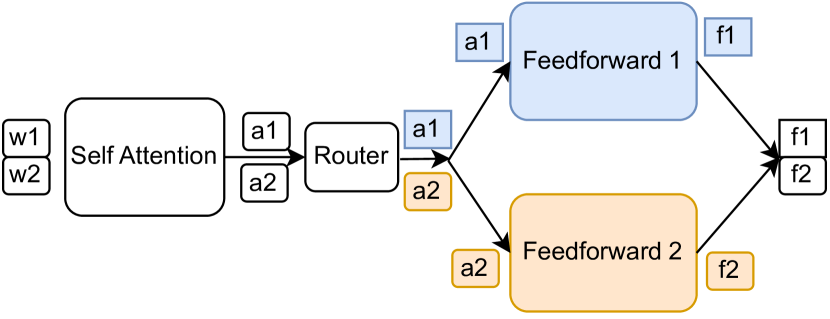
Figure 1. A single Mixture-of-Experts (MoE) layer with two “experts” or feedforward blocks. The input batch has two tokens, w1 and w2. We use the prefixes ‘w’, ‘a’, and ‘f’ to denote the input activations to the layer, output activations of self-attention and feedforward blocks respectively. Similarly we label each activation with an integer suffix corresponding to its token. Note that each token is uniquely routed to a single expert by a parameterized routing function.

Unfortunately, there is a limit to the improvements in model quality that can be achieved by simply increasing the number of experts (Shazeer et al., 2017). For example, in an experiment that studied the effect of adding experts to the T5 architecture (Raffel et al., 2019) as the base model, Fedus et al. observed diminishing improvements in the test set accuracy beyond 64-128 experts (Fedus et al., 2021). In fact, for training high quality Mixture-of-Experts models, it is imperative that the base models’ size (number of parameters) is increased along with the number of experts (Kim et al., 2021).

In this regard, current state-of-the-art distributed deep learning frameworks are inadequate for training such MoEs with large base models. They either support limited-sized base models or use inefficient parallel algorithms that lead to high communication costs. Hence, it is crucial to develop a distributed framework that can support the training of MoEs with large base models on multi-GPU clusters and do so efficiently, while keeping communication costs low. In this work, we present a three-dimensional, hybrid parallel framework, DeepSpeed-TED, that combines ZeRO’s data parallelism (Rajbhandari et al., 2020), MegatronLM’s tensor parallelism (Shoeybi et al., 2020), and DeepSpeed-MoE’s expert parallelism (Rajbhandari et al., 2022) to train MoE models that are built using extremely large base models. We demonstrate how the combination of these three dimensions of parallelism allows our framework to train 4–8 $\times$ larger base models compared to DeepSpeed-MoE (Rajbhandari et al., 2022), a state-of-the-art parallel framework that employs only two of these dimensions (data and expert). To the best of our knowledge, this is the first effort that combines these three state-of-the-art parallel deep learning algorithms for training MoEs on multi-GPU clusters.

We identify and resolve two bottlenecks that emerge with a naive combination of these three forms of parallelism. The first is a significant increase in memory usage in the optimizer, which limits the base model sizes supported by our hybrid parallel approach. To alleviate this issue, we propose a tiled version of the optimizer that processes model parameters in groups (or tiles) of fixed size, and decreases peak memory consumption by reusing GPU memory across the parameter tiles. The second bottleneck is related to communication costs, where a considerable amount of training time is spent in collective communication pertaining to expert and tensor parallelism. We identify two regions in this hybrid training procedure where messages are communicated unnecessarily among the worker GPUs, and propose novel communication optimizations that resolve this problem. For a 40 billion parameter MoE (6.7 billion base model with 16 experts) on 128 V100 GPUs of Summit, our optimizations reduce the overall collective communication time by 42% and lead to a significant improvement of 26% in the training time. DeepSpeed-TED is open source, and has been integrated in DeepSpeed, a state-of-the-art distributed deep learning framework.

The main contributions of this paper are as follows:

• A highly scalable first of its kind three-dimensional, hybrid parallel framework that combines ZeRO’s data (Rajbhandari et al., 2020), Megatron-LM’s tensor (Shoeybi et al., 2020), and DeepSpeed-MoE’s expert (Rajbhandari et al., 2022) parallelism to enable the training of Mixture-of-Experts with large base models.

• A tiled version of an optimizer that alleviates a significant memory spike in the optimizer step that arises from combining the three aforementioned forms of parallelism.

• Communication optimizations that eliminate unnecessary communication in our hybrid parallel algorithm which significantly reduce collective communication times.

2. Background

In this section, we provide a background on Mixture-of-Experts (MoE), and the three forms of parallelism used in this work – tensor parallelism (Shoeybi et al., 2020), expert parallelism (Rajbhandari et al., 2022), and data parallelism (Rajbhandari et al., 2020).

2.1. Mixture-of-Experts

Proposed by Shazeer et al. (Shazeer et al., 2017) in 2017, Mixture-of-Experts (MoEs) are a family of neural network architectures with an interesting property that their parameter set can be made arbitrarily large without increasing their computational costs. This is achieved by adding sparsely activated expert blocks to the layers of a dense neural network (called the base model). A parameterized routing function is added before these expert blocks that maps its input tokens to a unique expert. Since each token is computed upon by only one expert, the total computation cost of training remains fixed (same as the base model) and is independent of the number of experts. MoEs thus offer a unique way to increase the number of parameters of a given base model, and thus its performance on any task (Kaplan et al., 2020), without any increase in computational costs. Although Shazeer et al. used LSTMs (Hochreiter and Schmidhuber, 1997) as their base models, contemporary work on MoEs largely employ the transformer architecture (Vaswani et al., 2017) as the base models (Fedus et al., 2021; Lepikhin et al., 2020; Kim et al., 2021; Zuo et al., 2022; Xue et al., 2021; Dai et al., 2022; Du et al., 2022; Riquelme et al., 2021; Artetxe et al., 2021).

2.2. Data Parallelism and ZeRO

Under data parallelism, worker GPUs house a copy of the neural network and work on mutually exclusive shards of the input batch. After the backward pass they synchronize their local gradients via an all-reduce function call. However, a major limitation of data parallelism is that each GPU has to have enough memory to store the entire parameter set of a neural network, and also its gradients and optimizer states. To resolve this issue, Rajbhandari et al. proposed the Zero Redundancy Optimizer or ZeRO which is aimed at eliminating this redundant memory consumption in data parallel GPUs (Rajbhandari et al., 2020). Their method has three stages, which progressively save more memory albeit at the cost of increased communication. In this work, we consider the first stage of their optimization which only shards the optimizer states across data parallel ranks.

2.3. Expert Parallelism and DeepSpeed-MoE

After routing, the computation of an expert block of in an MoE layer is independent of other experts. Expert parallelism exploits this property by placing unique expert blocks on each GPU and computing them in an embarrassingly parallel fashion. Tokens are mapped to their corresponding experts by all-to-all communication within the participating GPUs. Due to its simplicity and effectiveness, expert parallelism is used in many parallel frameworks for training or running inference on MoEs (Nie et al., 2022; Shen et al., 2022; Fedus et al., 2021; Lepikhin et al., 2020; Artetxe et al., 2021). In this work, we use DeepSpeed-MoE’s implementation of expert parallelism (Rajbhandari et al., 2022).

2.4. Tensor Parallelism and Megatron-LM

Tensor parallelism involves partitioning the computation of a neural network layer across GPUs. Shoeybi et al. introduce MegatronLM, a tensor parallel algorithm to parallelize the computation of layers in a transformer neural network (Shoeybi et al., 2020). Their method is aimed at parallelizing a pair of consecutive fully-connected layers, which are found in the self-attention and feedforward blocks of the transformer (Vaswani et al., 2017). Their algorithm has seen significant adoption for training many large language models like Megatron-Turing NLG 530B (Smith et al., 2022), Bloom-176 B (BigScience, 2022), Turing NLG (Rajbhandari et al., 2020) etc.

3. TED: A Hybrid Tensor-Expert-Data Parallel Approach

By adding sparsely activated experts, the Mixture-of-Experts architecture allows us to make a given neural network, i.e. the base model, arbitrarily large while keeping its computation cost unchanged. However, merely increasing the number of experts yields diminishing returns in model generalization beyond 64–128 experts (Fedus et al., 2021). To build high quality MoEs, it is imperative that we increase the base model sizes as well as the number of experts (Kim et al., 2021). In this section, we provide an overview of TED, our hybrid parallel approach which combines DeepSpeed-MoE’s expert (Rajbhandari et al., 2022), MegatronLM’s tensor (Shoeybi et al., 2020) and ZeRO’s data (Rajbhandari et al., 2020) parallelism, to enable the training of such MoEs with extremely large multi-billion parameter base models on multi-GPU clusters. In this work, we use the first stage of ZeRO, which shards the optimizer states across data parallel GPUs. While further stages of their optimizations (stage-2, 3, offload (Ren et al., 2021) and infinity (Rajbhandari et al., 2021)) can support training of larger models, this happens at a cost to performance.

We use the terms non-expert and expert blocks interchangeably with self-attention and feedforward blocks respectively. Note that TED parallelizes the computation of expert and non expert blocks in a different manner. This is because expert parallelism is only applicable to the feedforward blocks of the transformer base model. Thus, TED uses a two dimensional hybrid of tensor and data parallelism to parallelize the non-expert blocks. Whereas, it utilizes all three of tensor, expert, and data parallelism for the expert blocks. Under TED, we organize available GPUs into two different virtual topologies for the non-expert and expert blocks. We illustrate these topologies in Figure 2.

Figure 2. TED uses a two dimensional hybrid of tensor and data parallelism to parallelize the computation of non-expert blocks. Whereas, it utilizes all three of tensor, expert, and data parallelism to parallelize expert blocks.

For the non-expert blocks, we maintain a two dimensional (2D) topology of GPUs, one dimension each for tensor and data parallelism. In this topology, GPUs in a row implement tensor parallelism, and we refer to a row of GPUs as a tensor parallel group. Similarly, TED realizes data parallelism across columns of GPUs, and we refer to these columns as data parallel groups. Likewise, for the expert blocks, we maintain a three dimensional (3D) topology of GPUs, one each for tensor, expert, and data parallelism. To form the tensor parallel groups for the expert blocks, we reuse the tensor parallel groups formed in the 2D topology for the non-expert blocks. However, we further decompose the data parallel groups of the non-expert blocks into a 2D topology to form groups for expert parallelism and data parallelism for the expert blocks. We define $\mathit{G_{tensor}}$ and $\mathit{G^{nonexp}_{data}}$ as the size of the tensor parallel and non-expert data parallel groups respectively. Similarly, we define $\mathit{G_{expert}}$ and $\mathit{G^{exp}_{data}}$ as the size of the expert parallel and expert data parallel groups respectively. Following prior work (Rajbhandari et al., 2020), we always set $\mathit{G_{expert}}$ to the number of experts in the model for performance considerations. Note that given a number GPUs, $\mathit{G}$, the following relation always holds true:

(1) $$\mathit{{G}_{tensor}}\times\mathit{G_{expert}}\times\mathit{G^{exp}_{data}}=\mathit{{G}_{tensor}}\times\mathit{G^{nonexp}_{data}}=G$$

In Figure 3, we illustrate the forward pass of an MoE layer with two experts on four GPUs. As mentioned previously, we set $\mathit{G_{expert}}$ to the number of experts i.e. 2. The other degrees of parallelism are $\mathit{{G}_{tensor}}=2$, $\mathit{G^{nonexp}_{data}}=2$, $\mathit{G_{expert}}=2$, and $\mathit{G^{exp}_{data}}=1$. We partition the parameters of the self-attention block (non-expert) and the two feed forward blocks (experts) as per the semantics of MegatronLM’s tensor parallelism and place the first partition on GPUs 0 and 2 and the second partition on GPUs 1 and 3. GPUs (0,1) and (2,3) thus form the two tensor parallel groups. GPU pairs (0,2) and (1,3) comprise the data parallel groups for the non-expert parameters. The same GPU pairs however comprise the expert parallel groups for the expert parameters. The four GPUs individually form singleton data parallel groups for the expert parameters.

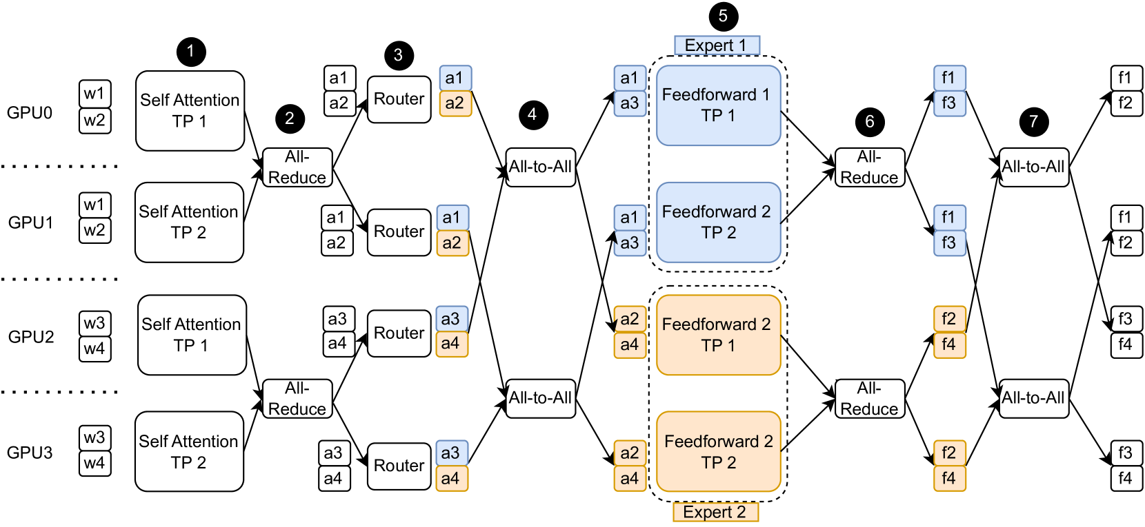
Figure 3. Forward pass of an MoE layer with two experts on four GPUs using TED. We use a $\mathit{{G}_{tensor}}\times\mathit{G^{nonexp}_{data}}=2\times 2$ topology for the non-expert self-attention blocks and $\mathit{{G}_{tensor}}\times\mathit{{G}_{expert}}\times\mathit{G^{exp}_{data}}=2\times 2\times 1$ topology for the expert feedforward blocks. We use the prefixes ‘w’, ‘a’, and ‘f’ to denote the input activations to the layer, output activations of self-attention and feedforward blocks respectively. Similarly we label each activation with an integer suffix corresponding to its token. Suffixes TP 1 and TP 2 denote the two tensor parallel partitions of the attention and feedforward blocks. The input batch consists of four tokens, with tokens 1 and 3 routed to the first expert (colored blue), and tokens 2 and 4 routed to the second expert (colored yellow).

Let us now discuss how our hybrid parallel algorithm computes the forward pass of an MoE layer. As an example, we use an input batch with four tokens (numbered 1-4) in Figure 3. The tensor parallel group of GPUs 0 and 1 compute on tokens 1 and 2, whereas the tensor parallel group of GPUs 2 and 3 compute on tokens 3 and 4. Each GPU first computes their partition of the self-attention block ( ) and then issues an all-reduce ( ) to aggregate the complete output activations (prefixed by ’a’) for their respective tokens. Now, each GPU applies the MoE routing function to their local tokens ( ). We assume that the routing function maps tokens 1 and 3 to the first expert i.e. feedforward 1, and tokens 2 and 4 to the second expert i.e. Feedforward 2. ( ) Now, an all-to-all communication primitive is issued in expert parallel groups to route the tokens as per the mapping decided by the routing function. Let us look at the expert parallel group of GPUs 0 and 2 to understand this all-to-all communication call. On GPU 0, token 1 has been mapped to the first expert and token 2 has been mapped to the second expert. Therefore, we want to retain a1 and send a2 to GPU 2 which houses the second expert. Similarly, on GPU 2, we want to retain a4 and send a3 over to GPU 0. Note that this communication pattern matches the semantics of an all-to-all communication primitive exactly. After the all-to-all has completed each GPU computes their tensor-parallel partitions of the expert feed forward blocks ( ) and issue an all-reduce to aggregate the complete output ( ). The final all-to-all communication call in the expert parallel groups ( ) essentially inverts the first all-to-all ( ) and brings back the tokens to their original GPUs. This is how our three dimensional hybrid parallel approach computes the forward pass of an MoE layer.

During the backward pass computation proceeds in the reverse direction i.e. ( - ). The all-to-all communication at and calls are reversed. For example, consider , wherein the input to the all-to-all on GPU 0 would be gradients of the loss w.r.t. f1 and f2. Similarly for GPU 2, it would be the gradients w.r.t.  f3 and f4. Now, after the all-to-all, the outputs on GPU 0 would be gradients of the loss w.r.t f1 and f3, and on GPU 2 it would be gradients of the loss w.r.t. f2 and f4. The all-reduce function calls ( , ) are applied to the gradients w.r.t the input activations instead of the output. For more details about this all-reduce call, we refer the reader to Narayanan et al. (Narayanan et al., 2021). Note that total amount of communication i.e. two all-reduces and two all-to-alls is the same as that of the forward pass. Finally, the data parallel groups synchronize their gradients via another all-reduce call, which completes the backward pass.

3.1. A Model for Memory Consumption

We now derive the extent to which TED can increase the base model sizes as compared to prior work like DeepSpeed-MoE (Rajbhandari et al., 2022), which only employ data and expert parallelism. Following previous work, we assume that every alternate layer has expert feedforward modules (Lepikhin et al., 2020; Fedus et al., 2021; Kim et al., 2021). Let $\mathit{NP_{base}}$ denote the number of parameters in the base model and $E$ denote the number of experts. Let $G$ be the number of GPUs. Note that two-thirds of the parameters in the base model reside in feed-forward blocks, and the remaining one-third in self-attention blocks (Narayanan et al., 2021). Since only half of the feedforward blocks are designated as experts, the total number of expert parameters, $\mathit{NP_{exp}}$, in an MoE model are:

(2) $$\mathit{NP_{exp}}=E\times\frac{1}{2}\times\left(\frac{2}{3}\times\mathit{NP_{base}}\right)=\frac{E}{3}\times\mathit{NP_{base}}$$

Now, the non-expert parameters are comprised of parameters in all the self-attention blocks and half of the feed-forward blocks. Thus, the total number of non-expert parameters, $\mathit{NP_{nonexp}}$, is

(3) $$\mathit{NP_{nonexp}}=\frac{1}{2}\times\left(\frac{2}{3}\times\mathit{NP_{base}}\right)+\frac{1}{3}\times\mathit{NP_{base}}=\frac{2}{3}\times\mathit{NP_{base}}$$

Rajbhandari et al. (Rajbhandari et al., 2020) prove that the lower bound of memory consumption per GPU with ZeRO stage-1 is $\left(4+\frac{12}{\mathit{G_{data}}}\right)\times\mathit{NP_{gpu}}$, where $\mathit{G_{data}}$ is the degree of data parallelism and $\mathit{NP_{gpu}}$ is the number of parameters of the model per GPU. Now, we use this formulation to derive a lower bound on memory consumption per GPU for TED as follows:

(4) $$\mathit{M_{gpu}}\geq\left(4+\frac{12}{\mathit{G^{nonexp}_{data}}}\right)\times\mathit{NP^{nonexp}_{gpu}}+\left(4+\frac{12}{\mathit{G^{exp}_{data}}}\right)\times\mathit{NP^{exp}_{gpu}}$$

Here, $\mathit{NP^{nonexp}_{gpu}}$ and $\mathit{NP^{exp}_{gpu}}$ are the number of expert and non expert parameters per GPU. As discussed previously, $\mathit{G^{nonexp}_{data}}$ and $\mathit{G^{exp}_{data}}$ are the degrees of data parallelism for the non-expert and expert blocks respectively. Now, let us try to derive the values of $\mathit{NP^{nonexp}_{gpu}}$ and $\mathit{NP^{exp}_{gpu}}$, starting with the former. MegatronLM’s tensor parallelism divides the parameters of a model equally among the GPUs in a tensor parallel group. Since the size of a tensor parallel group in TED is $\mathit{G_{tensor}}$, we can write $\mathit{NP^{nonexp}_{gpu}}=\frac{\mathit{NP_{nonexp}}}{\mathit{G_{tensor}}}$. However, the expert parameters are divided within both the tensor parallel and expert parallel groups. As discussed previously, we use a degree of expert parallelism equal to the number of experts i.e. $\mathit{G_{expert}}=E$. Thus, $\mathit{NP^{exp}_{gpu}}=\frac{\mathit{NP_{exp}}}{\mathit{G_{tensor}}\times E}$. Also, it follows from Equation 1 that $\mathit{G^{nonexp}_{data}}=\frac{\mathit{G}}{\mathit{G_{tensor}}}$ and $\mathit{G^{exp}_{data}}=\frac{\mathit{G}}{\mathit{G_{tensor}}\times\mathit{G_{expert}}}=\frac{\mathit{G}}{\mathit{G_{tensor}}\times\mathit{E}}$. Substituting these values in Equation 4, we get

$$\mathit{M_{gpu}} \geq\left(4+\frac{12\mathit{G_{tensor}}}{G}\right)\times\frac{\mathit{NP_{nonexp}}}{\mathit{G_{tensor}}}+\left(4+\frac{12\mathit{G_{tensor}}E}{G}\right)\times\frac{\mathit{NP_{exp}}}{\mathit{G_{tensor}}E}$$

$$\geq\frac{4}{\mathit{G_{tensor}}}\left(\mathit{NP_{nonexp}}+\frac{\mathit{NP_{exp}}}{E}\right)+\frac{12}{G}(\mathit{NP_{nonexp}}+\mathit{NP_{exp}})$$

Now substituting from Equation 2 and 3, we get

$$\mathit{M_{gpu}} \geq\frac{4}{\mathit{G_{tensor}}}\left(\frac{2}{3}\mathit{NP_{base}}+\frac{\mathit{NP_{base}}}{3}\right)+\frac{12}{G}(\frac{2}{3}\mathit{NP_{base}}+\frac{E}{3}\mathit{NP_{base}})$$

$$\geq\frac{4\mathit{NP_{base}}}{\mathit{G_{tensor}}}+\frac{4(E+2)}{G}\mathit{NP_{base}}$$

(5) $$\geq 4\mathit{NP_{base}}\times\left(\frac{1}{\mathit{G_{tensor}}}+\frac{E+2}{G}\right)$$

Equation 5 can be used to derive an upper bound on the largest possible base model size that our framework can train, given enough number of GPUs. Note that as we increase the number of GPUs involved in training, the second term becomes negligible compared to the first. This gives us,

$$\mathit{M_{gpu}} \geq\frac{4\mathit{NP_{base}}}{\mathit{G_{tensor}}}$$

(6) $$\implies\mathit{NP_{base}} \leq\frac{\mathit{G_{tensor}}}{4}\times\mathit{M_{gpu}}$$

Note that substituting $\mathit{G_{tensor}}=1$ in Equation 6 gives us the base model upper bound for Rajbhandari et al. (Rajbhandari et al., 2022), the current state-of-the-art for training MoEs. Thus, we have shown that our system enables the training of $\mathit{G_{tensor}}\times$ larger base models compared to the previous state-of-the-art. Note that the maximum degree of tensor parallelism is limited to the number of GPUs in a node due to performance considerations (Narayanan et al., 2021). Nevertheless, our framework can still support $4\times$, $6\times$ and $8\times$ larger base models on Perlmutter, Summit and an NVIDIA-DGX-A100 machine respectively.

4. Memory Savings via Tiling

In the previous section, we provided an overview of how TED distributes the parameters and the computation of the forward and backward passes across the GPUs. However, a naive combination of tensor, expert, and data parallelism leads to significant spikes in memory usage during the optimizer step. Interestingly, the magnitude of this spike becomes worse as we increase the number of experts and/or the base model sizes. Note that it is important to resolve this issue so that we are able to fit MoEs with large base models in memory. Below, we discuss this phenomenon in detail and outline our solution to resolve this issue.

To demonstrate the aforementioned memory usage spike, we profile the memory consumed per GPU during various phases of training (forward pass, backward pass, optimizer step) for an MoE model with a 2.7B parameter base model and 32 experts, and show the results in Figure 4. We run this experiment on 32 GPUs of an NVIDIA DGX-A100 cluster with eight GPUs per node. We set the degree of tensor and expert parallelism to 1 and 32 respectively. This results in degrees of data parallelism as 32 and 1 for the non-expert and expert blocks respectively. We observe that memory consumption peaks during the optimizer step with a very significant spike of around 4.5 GB. An intermediate step in the optimizer phase in mixed precision training is the up-casting of 16-bit gradients to 32-bit gradients before the optimizer updates the weights. This requires the creation of a temporary buffer to store the 32-bit gradients and is exactly the reason why there is a significant increase in memory consumption. In fact, this problem becomes worse with increasing base model sizes and/or expert counts. Let us now understand why.

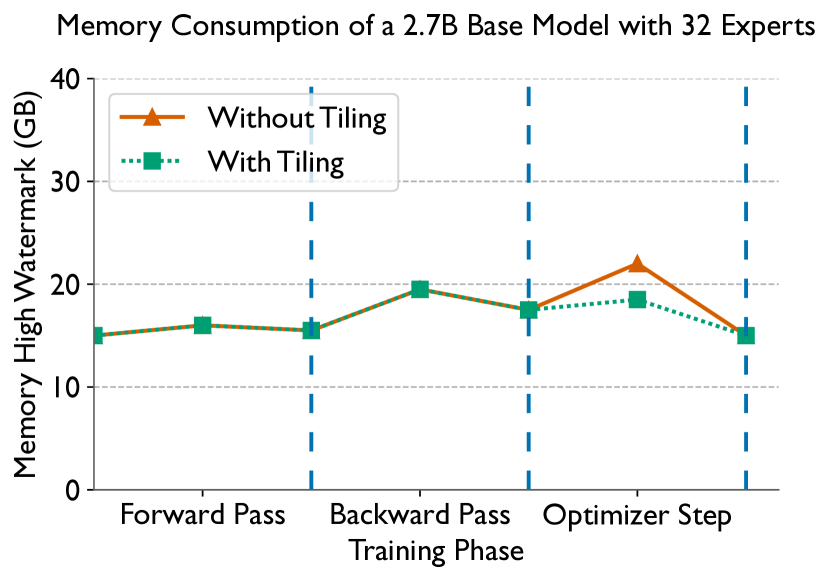
Figure 4. Memory consumption in the various phases of training for an MoE with a 2.7B parameter base model and 32 experts on 32 GPUs of an NVIDIA DGX-A100 (40 GB) cluster. We observe a large spike of an additional 4.5 GB in memory usage during the optimizer step (red), which is significantly reduced to around 1.5 GB by our tiled optimizer (green).

TED uses ZeRO stage-1 which reduces memory consumption by sharding the optimizer states and computation across the data parallel groups. Greater the degree of data parallelism, the greater the reduction in memory consumption (Rajbhandari et al., 2020). From the discussion in Section 3, we know that TED employs different degrees of data parallelism for the expert parameters and non-expert blocks. In fact, it follows from Equation 1 that

$$\mathit{{G}_{tensor}}\times\mathit{G_{expert}}\times\mathit{G^{exp}_{data}} =\mathit{{G}_{tensor}}\times\mathit{G^{nonexp}_{data}}$$

$$\mathit{G_{expert}}\times\mathit{G^{exp}_{data}} =\mathit{G^{nonexp}_{data}}$$

$$\mathit{E}\times\mathit{G^{exp}_{data}} =\mathit{G^{nonexp}_{data}}$$

(7) $$\mathit{G^{exp}_{data}} =\frac{\mathit{G^{nonexp}_{data}}}{\mathit{E}}$$

From Equation 7, we can conclude that the degree of data parallelism for the expert blocks is $\mathit{E}\times$ less than that for the non-expert blocks. Therefore, ZeRO provides lesser memory savings for the expert blocks than the non expert blocks. This is because the optimizer states for the expert blocks are sharded over $\mathit{E}\times$ lesser GPUs. Thus, as $\mathit{E}$ increases each GPU has to process increasing number of parameters in the optimizer step. This leads to an increase in the size of the temporary 32-bit gradient buffer required to up-cast the expert parameter gradients. Increasing the base model size also worsens this problem as the size of the expert parameter group is directly proportional to the base model size. This is why it is imperative to resolve this issue such that we can train MoEs with large base models and/or large number of experts.

In this work, we propose a tiled formulation of the optimizer that strives to alleviate the aforementioned issue. Instead of processing the entire expert parameter group at once, we propose partitioning these parameters into “tiles” of a predefined size and iteratively processing these tiles. This ensures that at any given time, temporary 32-bit gradients are only produced for parameters belonging to a given tile. The temporary memory used to store these gradients can in fact be reused across tiles. For a tile size $\mathit{ts}$, we now only need $4\times\mathit{ts}$ bytes of memory to materialize the 32-bit gradients. This makes the optimizer memory spike independent of the number of experts and the base model sizes! In our experiments, we fix the tile size to 1.8 million parameters, which essentially caps the spike in the optimizer step to 1 GB. We observed that this tile size is large enough to not cause any performance degradation due to the latency of multiple kernel launches. In Figure 4, we demonstrate how our tiled optimizer reduces the per GPU peak memory consumption for the aforementioned MoE with a 2.7B parameter base model and 32 experts by 3 GB. In fact, on another MoE with 6.7B parameters and 16 experts on 32 GPUs, our framework ran out of memory without tiling. Whereas, with tiling enabled, we were able to successfully train this model with a peak memory consumption of 31.3 GB. Since the maximum memory capacity of these GPUs is 40 GB, optimizer tiling provides a significant memory savings of more than 21.75%!

5. Performance Optimizations

In the preceding sections, we focused on increasing the maximum possible size of MoEs that are supported by our framework. While the memory savings provided by expert and tensor parallelism contribute to this, they also result in a significant portion of the batch time being spent in expensive collective communication. In Figure 3, we can observe that the forward pass includes two all-reduce calls within the tensor parallel groups, and two all-to-all calls within the expert parallel groups. During the backward pass, these calls are repeated again. Also, large model training almost always uses activation checkpointing (Chen et al., 2016), which significantly reduces activation memory at the expense of a duplicate forward pass per layer. Thus, overall we end up with six all-to-all and six all-reduce communication calls, which become a significant bottleneck in training. We empirically demonstrate this in Figure 5 (leftmost bar titled Baseline), wherein we observe that almost half of the batch time is spent in the all-to-all and all-reduce communication calls. We will now describe two performance optimizations that seek to reduce the time spent in these communications and are extremely critical to the performance of our framework.

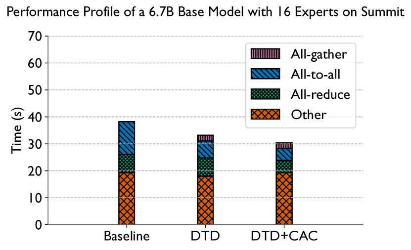
Figure 5. Impact of our communication optimizations on the batch time of an MoE model with a 6.7B parameter base model and 32 experts on 128 GPUs of Summit (batch size: 1024). Our optimizations result in significant reductions of 64.12% and 33% in the all-to-all and all-reduce time respectively, thereby improving the overall training time by 20.7%.

5.1. Duplicate Token Dropping (DTD) for Reducing Communication Volume

MegatronLM’s tensor parallelism for partitioning self-attention and feed forward blocks involves issuing an all-reduce on local partial outputs to materialize the full outputs on each rank (Shoeybi et al., 2020). For example, in Figure 3, GPUs 0 and 1 issue an all-reduce ( ) after the self-attention block to assemble the full self-attention outputs for tokens 1 and 2. While, this leads to duplication of activations across the tensor parallel ranks, it is not an issue for training regular transformer models (i.e. without experts) as the tensor parallel blocks under MegatronLM’s algorithm require a complete set of input activations on each tensor parallel rank. Thus the duplicate activations output by a tensor parallel block serve as the required input for its successor. However, for MoEs, an unwanted side effect of this design choice is the presence of redundant tokens in the all-to-all communication calls. For example consider the first all-to-all in Figure 3 ( ). Self-attention output activations, a1 and a2, are communicated by both GPUs 0 and 1. Similarly, GPUs 2 and 3 both communicate a3 and a4. In general, the amount of unnecessary data in the all-to-all communication calls for a given token is proportional to the degree of tensor parallelism. Thus, naively combining expert and tensor parallelism can lead to the all-to-all communication becoming a significant bottleneck, especially as we try to increase the base model sizes (larger base models need more tensor parallelism). For example, in Figure 5, 32% of the batch time is spent in the all-to-all (leftmost bar titled baseline)! The degree of tensor parallelism and thus the degree of redundancy in the all-to-alls is four here.

To resolve this bottleneck, we propose duplicate token dropping (DTD), a communication optimization geared towards eliminating unnecessary data in the all-to-all communication. We illustrate the working of DTD in Figure 6 for the first all-to-all communication in an MoE layer ( in Figure 3). Before the all-to-all is issued, GPUs within tensor parallel groups participate in a “drop” operation ( in Figure 6). The drop operation ensures that the there is no redundancy in the output activations across the tensor parallel ranks. For instance, GPU 0 drops the activation of a2 whereas GPU 1 drops the activation a1, thereby completely eliminating redundancy within their tensor parallel group. Similarly, GPUs 3 and 4 drop a3 and a4 respectively. The drop operation thus reduces the all-to-all message sizes by two times in this example, and in general the reduction is equal to the degree of tensor parallelism. However, after the all-to-all, the GPUs do not have the full input activations to commence the computation of the expert feed forward blocks. For instance, GPU 0 has the input activations for the token 1, but not for token 3 and vice versa for GPU 1. Therefore, to assemble the full input activations, we issue an all-gather call ( in Figure 6) between the tensor parallel GPUs. The all-gather ensures that the input dependencies for the expert feedforward blocks are met.

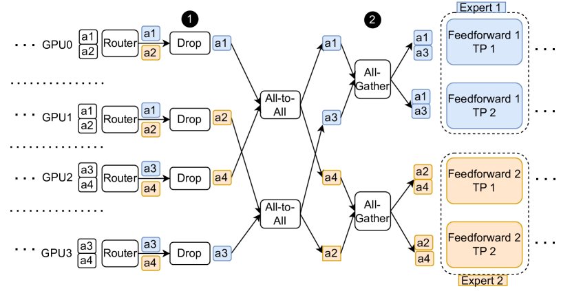
Figure 6. Duplicate token dropping (DTD) in the first all-to-all communication of an MoE layer (Steps 3–5 in Figure 3). Before the all-to-all, we apply the drop operation, which eliminates redundant tokens across tensor parallel ranks, and reduces the all-to-all message sizes by the degree of tensor parallelism. After the all-to-all, GPUs reassemble the full input to the feed forward blocks by issuing an all-gather between the tensor parallel ranks.

During the backward pass the all-gather call is replaced by a drop operation and the drop operation is replaced by an all-gather call. For the MoE model in Figure 5, we observe that DTD reduces the all-to-all communication time by 48%. While the inclusion of DTD leads to an additional all-gather operation (shown in red on top of the second bar), this overhead is outweighed by the improvement in the all-to-all communication timing. Overall, DTD results in an improvement of 13.21% in the batch time.

5.2. Communication-aware Activation Checkpointing (CAC)

We now turn our attention to a second source of redundant communication in large model training, namely activation checkpointing (Chen et al., 2016). Intermediate activations in a neural network generated during the forward pass need to be stashed in memory as they are required during the backward pass for the gradient computation. However, for large model training, storing all the activations can lead to tremendous memory overhead. Activation checkpointing alleviates this issue by storing only a subset of the activations, which are essentially just the input activations of every layer. During the backward pass of a layer, the remaining activations are re-materialized from its stashed input activation by doing a local forward pass for that layer. Thus, activation checkpointing saves activation memory at the expense of a duplicate forward pass for every layer, and is almost always used for training large neural networks. For more details, we refer the reader to Chen et al. (Chen et al., 2016).

We know from Section 3 that the forward pass of an MoE layer in TED involves two all-to-alls and two all-reduce calls in the forward pass and two all-to-alls and two all-reduce calls in the backward pass. Since activation checkpointing involves repeating the forward pass of a layer, we now end up with two additional all-to-all and all-reduce calls, thereby increasing communication volume by $1.5\times$ and making the training process inefficient.

To this end, we propose communication-aware checkpointing (CAC), a communication optimization that eliminates the additional communication in the second forward pass induced by activation checkpointing. During the first forward pass, CAC stashes the outputs of each all-reduce and all-to-all communication call along with the data stashed by standard activation checkpointing. Now, during the second forward pass, we bypass these communication calls and instead return the outputs for these communication calls stashed during the first forward pass. CAC thus reduces the communication volume by 33% at the expense of using extra GPU memory. For the MoE model in Figure 5, CAC indeed reduces the all-to-all and all-reduce communication times by 33% (compare second and third bars). In combination with DTD, the reductions in the all-to-all and all-reduce communication times are 64.12% and 33% respectively, amounting to a speedup of nearly 20.7% over the baseline version of DeepSpeed-TED.

6. Experimental Setup

This section provides an overview of the empirical evaluation of DeepSpeed-TED. Our framework is open source, and has been integrated in DeepSpeed, a state-of-the-art framework for parallel deep learning. We conduct our experiments on the Summit and ThetaGPU supercomputers. Summit has six 16 GB NVIDIA V100 GPUs per node, each having a peak half precision throughput of 125 Tflop/s. Each node has two 22-core Power 9 CPUs. The peak intra-node and inter-node GPU bidirectional communication bandwidths are 50 GB/s (NVlink) and 25 GB/s (Infiniband) respectively. On the other hand, ThetaGPU is a NVIDIA DGX A100 machine with eight 40 GB NVIDIA A100 GPUs per node, each having a peak half precision throughput of 312 Tflop/s. On this machine, the peak intra-node and inter-node GPU bidirectional communication bandwidths are 600 GB/s (NVlink) and 200 GB/s (Infiniband) respectively.

6.1. Neural Network Architectures and Datasets

Table 1 lists the various base model architectures used in this study. All MoEs used in our empirical experiments are constructed by adding expert blocks to every alternate layer of one of these base models (this is in line with previous work (Lepikhin et al., 2020; Fedus et al., 2021; Kim et al., 2021)). The base models and their corresponding hyperparameters are taken from Brown et al. (Brown et al., 2020). We use the Pile dataset to generate input tokens (Gao et al., 2021). We use the AdamW optimizer (Loshchilov and Hutter, 2017), which is the standard practice for large language model training. We implement the layers of our transformer models using MegatronLM’s GPU kernels (Shoeybi et al., 2020).

Table 1. Architectural details and batch sizes for the various transformer base models used to build the MoEs used in this study. All hyperparameters including the batch sizes are taken from Brown et al. (Brown et al., 2020).

# Parameters	# Layers	Hidden Size	Attention Heads	Batch Size
1.3B	24	2048	16	512
2.7B	32	2560	32	512
6.7B	32	4096	32	1024
13.0B	40	5140	40	2048

First, we establish the correctness of our implementation by training a 2.6B parameter MoE model (1.3B parameter base model and 4 experts) to completion on the BookCorpus dataset (Zhu et al., 2015), on 8 GPUs, and present the validation loss curves. For reference, we also train this model using DeepSpeed-MoE (Rajbhandari et al., 2022), the current state-of-the-art framework for training MoEs and compare the two loss curves. Then, we demonstrate the maximum MoE model sizes that our framework can support for a given number of GPUs and compare it with DeepSpeed-MoE (Rajbhandari et al., 2022). Next, we conduct strong scaling studies using MoEs built from the 1.3B, 2.7B and 6.7B parameter transformer models in Table 1 on 32 to 256 GPUs. At 32 GPUs, we add as many experts as the system memory permits. We strong scale a model in two ways, first increasing the number of GPUs while keeping the number of experts constant, and second by varying the number of experts proportional to the number of GPUs. Note that even though the latter experiment increases the model size with scale, it is still considered strong scaling as adding experts to a base model does not change the total number of floating point operations in training. For our weak scaling runs, we fix the number of experts to 16 and use base models of increasing sizes from Table 1 as we go from 32 to 256 GPUs. Note that this is weak scaling, because the number of floating point operations are proportional to the base model size.

6.2. Evaluation Metrics

We illustrate the results of our experiment using the average time per iteration (or batch). To calculate this, we first run a given model with 100 batches sampled from the Pile dataset (Gao et al., 2021) and take the average of the last 90. We do not include the first 10 batches because PyTorch issues expensive mem-alloc calls to the CUDA runtime in the initial iterations to reserve enough memory for training. We also derive the percentage of peak half-precision throughput from the average batch time using Narayanan et al.’s formulation(Shoeybi et al., 2020). Note that this an analytical formulation of the total number of flop/s (and thus the percentage of peak half-precision throughput). Since Narayanan et al.’s formulation is a lower bound on the total floating point operations, we expect empirically measured flop/s to be higher.

7. Results

In this section, we discuss the results of the empirical experiments outlined in Section 6.

7.1. Validating Our Implementation

To verify the correctness of DeepSpeed-TED, we train an MoE with a 1.3B parameter base model and 4 experts on 8 GPUs of ThetaGPU and present the validation loss curve in Figure 7. We set $\mathit{G_{tensor}}=2$, $\mathit{{}_{expert}}=4$, $\mathit{G^{nonexp}_{data}}=4$, and $\mathit{G^{exp}_{data}}=1$. This allows us to test the correctness of our framework in a scenario where all three dimensions of its hybrid parallel approach are active. We also enable the communication optimizations discussed in Section 5 i.e. DTD and CAC. We observe that our framework is able to successfully train the model to convergence, and produces identical loss curves to DeepSpeed-MoE, a system that has been previously used to train state-of-the-art MoE models. In this way, we establish the correctness of our implementation.

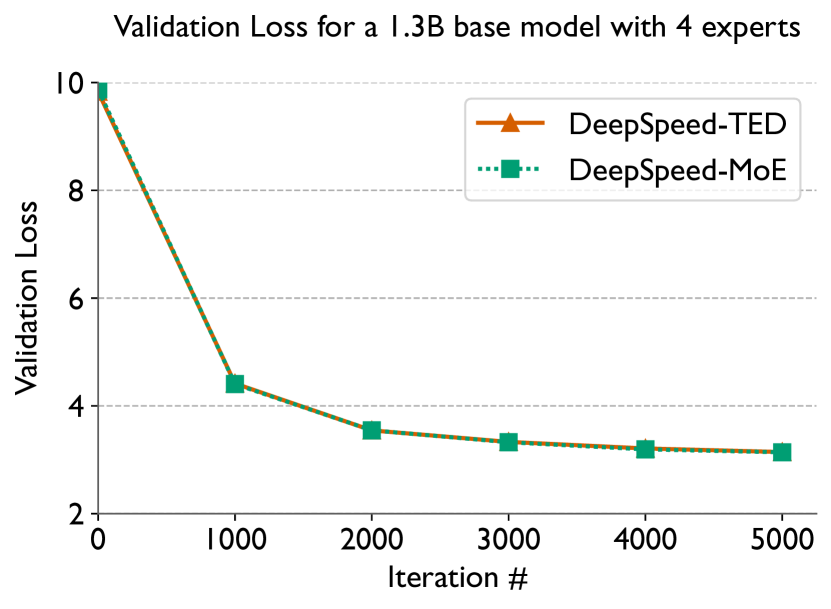
Figure 7. Validation loss for an MoE with a 1.3B base model and four experts on eight GPUs of ThetaGPU on the BookCorpus dataset (Zhu et al., 2015). We use a batch size of 128 and sequence length of 2048. We set $\mathit{G_{tensor}}=2$, $\mathit{G_{expert}}=4$, $\mathit{G^{exp}_{data}}=1$, $\mathit{G^{nonexp}_{data}}=4$.

7.2. Comparison of Supported Model Sizes

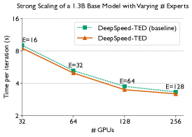
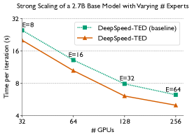
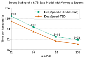
Figure 8. Strong scaling (with varying number of experts) of MoEs with the 1.3B, 2.7B and 6.7B parameter models in Table 1 used as base, on V100 GPUs of Summit. We annotate the plot with the number of experts used at each GPU count. We sample input batches of sizes 512, 512 and 1024 respectively, from the Pile dataset(Gao et al., 2021).

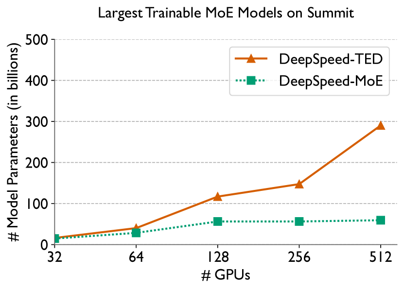
Figure 9. Largest MoE model sizes supported on various GPU counts on Summit. We construct MoEs using base models from Table 1 and number of experts in the range of 4 to 128. Compared to DeepSpeed-MoE (Rajbhandari et al., 2022), our framework supports 1.09-4.8$\times$ larger MoE models, with the ratio increasing with increasing number of GPUs.

Figure 9 illustrates the results of our experiment in which we benchmark the largest MoE models that our framework and DeepSpeed-MoE (Rajbhandari et al., 2022) can train without running out of memory for various GPU counts ranging between 32 and 512. We use the base models in Table 1. To make sure that the experiment is fair to both the frameworks we do two things. While our proposed approach can in theory support arbitrarily large base models by increasing the degree of tensor parallelism, it is well known that tensor parallelism is extremely inefficient when used across nodes. Therefore, we only allow our framework to use a maximum tensor parallel degree of six, which is the number of GPUs on a node of Summit. Second, we limit the largest possible number of experts to 128 as prior work has demonstrated limited improvements in the statistical efficiency of a model beyond this number (Fedus et al., 2021).

Across the range of GPUs used in this experiment, we observe that DeepSpeed-TED supports $1.09-4.8\times$ larger MoE models than DeepSpeed-MoE. We also observe that this ratio increases as we increase the number of GPUs. This can be explained by Equation 5, which states that the memory consumption of our approach decreases with increasing number of GPUs. We observe that beyond 128 GPUs, our proposed framework can train MoEs with hundreds of billion of parameters on Summit, which is not possible with DeepSpeed-MoE. Thus, we have empirically demonstrated how our DeepSpeed-TED can enable the development of high quality MoE models, the parameters of which have been scaled along the base model dimension as well as the expert dimension.

7.3. Strong Scaling Performance

We now discuss the results of our strong scaling experiments, starting with the runs that varied the number of experts proportional to the number of GPUs. We demonstrate the results for the 1.3B, 2.7B and 6.7B base models in Figure 8. To demonstrate the efficacy of the communication optimizations discussed in Section 5, we also benchmark the baseline version of our framework i.e. with DTD+CAC disabled, and call it DeepSpeed-TED (baseline). Across all the figures, we observe that augmenting the training procedure with DTD and CAC indeed improves the hardware efficiency of training. However, while the speedups for the 2.7B and 6.7B parameter base models are significant: 19 to 23% and 25 to 29% respectively, our communication optimizations seem to be less effective for the smallest 1.3B base model providing modest speedups of around 4 to 7%. This is because at the given GPU counts and number of experts, ZeRO’s memory optimizations and expert parallelism are able to fit this model in memory without the aid of tensor parallelism. Without tensor parallelism there is no redundancy in the all-to-all communication (see Section 5.1) and thus the DTD communication optimization is of no use in this scenario. Similarly, without tensor parallelism there is no all-reduce communication ( and of Figure 3). Thus, CAC only eliminates the unnecessary all-to-all calls, and is only partially applicable to this scenario. This explains the reduced effectiveness of our optimizations for the 1.3B base model.

Unlike the 1.3B base model, the 2.7B and 6.7B model require a tensor parallel degree of 2 and 4 to fit in available GPU memory. The ensuing redundancy in the all-to-all messages and the introduction of tensor parallelism thus makes our communication optimizations quite effective. Again, we observe larger speedups for the MoEs using the 6.7B base model (25–29% versus 19–23%) as a higher degree of tensor parallelism implies more redundancy in the all-to-all messages, which our optimizations successfully eliminate. It also implies a larger proportion of time spent in tensor parallel all-reduces which is significantly reduced by CAC.

In our strong scaling runs with fixed number of experts, we observed very similar absolute times per iteration and relative speedups for all the three models. For brevity, we only include the results for the 6.7B parameter base model, and illustrate them in Figure 10. We have thus verified that our optimizations are effective at improving performance in two strong scaling setups across various base model sizes.

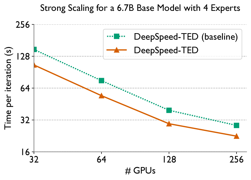
Figure 10. Strong scaling (with number of experts fixed to four) of a MoE with a 6.7B parameter model in Table 1 used as base, on V100 GPUs of Summit. We sample input batches of size 1024 from the Pile dataset(Gao et al., 2021).

7.4. Weak Scaling Performance

As discussed in Section 6, we conduct a weak scaling experiment by fixing the number of experts to 16 and varying the base model size in proportion with the number of GPUs. We demonstrate the time per iteration (or batch) and percentage of peak half-precision throughputs for this experiment in Figure 11 and Table 2 respectively. Again, we observe a minor speedup of 6% for the 1.3B base model, and significant speedups of 20%, 25% and 36% for the 2.7B, 6.7B and 13B base models respectively. Just like the previous section, the progressively increasing effectiveness of our communication optimizations for larger base models can be explained by the correspondingly increasing degrees of tensor parallelism - 1, 2, 4, and 8. This creates more redundancy for the larger models in the all-to-all and increases the net communication volume of the all-reduces. Note that while the speedups for the 13B parameter model is significant (36%), the hardware utilization for this model is extremely low. Even with our optimizations, we are only able to achieve 11.7% of the peak half-precision flop/s, which is significantly lower than the 1.3B (37% of peak), 2.7B (30% of peak) and 6.7B (27% of peak) base models. The explanation for this observation is that a tensor parallel degree of 8 for this model is greater than the number of GPUs on a Summit node. This experiment corroborates prior work which has observed that Megatron-LM’s algorithm does not scale well beyond the confines of a node (Narayanan et al., 2021; Singh and Bhatele, 2022).

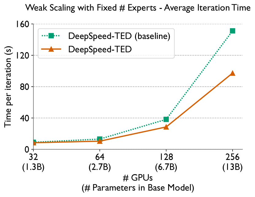
Figure 11. Average time per iteration (left) for a weak scaling study of MoE models with 16 experts on Summit. Base models and batch sizes are taken from Table 1.

Table 2. Percentage of peak half precision throughput for a weak scaling study of MoE models with 16 experts on Summit. Base models and batch sizes are taken from Table 1.

	Base Model Size	Throughput
# GPUs	(# Parameters)	(% of peak)
32	1.3B	36.7
64	2.7B	30.0
128	6.7B	26.2
256	13.0B	11.7

8. Related Work

Due to the increasing computational costs of training state-of-the-art neural networks, several frameworks and algorithms have been proposed that can train these networks in parallel on networked multi-GPU clusters. These can broadly be divided intro three categories - data, tensor, and pipeline parallelism. Under data parallelism, participating GPUs are assigned a full copy of the neural network. The parallelism comes from the fact that each GPU works on a equal sized shard of the input batch at every iteration. Perhaps due to its simplicity of implementation, data parallelism has been the most widely adopted algorithm and can be found in popular deep learning frameworks like PyTorch (as Distributed Data Parallel (Li et al., 2020)). However, a major limitation of data parallelism is that it requires the full neural network to fit on each GPU. To resolve this issue, Rajbhandari et al. propose the Zero Redundancy Optimizer (ZeRO) which shards the parameters, gradients, and/or optimizer states of the model across participating GPUs (Rajbhandari et al., 2020), and enable training of much larger models that far exceed the memory capacity of a single GPU. PyTorch also natively offers Fully Sharded Data Parallelism (FSDP), which is based off a similar idea (Zhao et al., 2023).

Tensor parallel algorithms like MegatronLM (Shoeybi et al., 2020) divide the parameters and computation of each layer of a neural network across participating GPUs and can thus also be used to train neural networks that do not fit on a single GPU. Other examples of tensor parallel frameworks and algorithms are  (Xu et al., 2021; Wang et al., 2022; Bian et al., 2021) for fully connected layers,  (Dryden et al., 2019a, b) for convolution layers, and  (Tripathy et al., 2020) for graph neural networks. On the other hand, pipeline parallelism involves assigning the parameters and computation of a contiguous subset of layers to each GPU (Huang et al., 2019; Narayanan et al., 2021; Microsoft, 2021; Tanaka et al., 2021; Singh and Bhatele, 2022). Parallelism is achieved by breaking a batch into microbatches and processing the microbatches in a pipelined fashion (akin to pipelining in computer architecture). Narayanan et al. show how combining tensor, pipeline, and data parallelism can be an extremely efficient strategy to train large multi-billion parameter models at scale (Narayanan et al., 2021). As future work, we plan to integrate pipeline parallelism in DeepSpeed-TED to further enhance its performance.

To combat the rising computation costs of training state-of-the-art neural networks like Chinchilla (Hoffmann et al., 2022), GPT-3 (Brown et al., 2020), and Megatron-Turing NLG (Smith et al., 2022), the machine learning community has recently turned its attention to the Mixture-of-Experts (MoE) architecture to train large compute efficient transformer models for natural language processing and computer vision (Fedus et al., 2021; Du et al., 2022; Riquelme et al., 2021; Lepikhin et al., 2020). Subsequently, a number of parallel deep learning frameworks have been proposed for training or running inference on MoEs on multi-GPU clusters. These frameworks usually combine the aforementioned parallel deep learning algorithms with expert parallelism, which entails computing expert blocks in an embarrassingly parallel manner on multiple GPUs. Rajbhandari et al. present DeepSpeed-MoE (Rajbhandari et al., 2022), a state-of-the-art system for training and running inference on MoEs that combines expert parallelism with ZeRO’s data parallelism. Nie et al. combine develop highly optimized kernels for routing and all-to-all communication in their framework called HetuMoE (Nie et al., 2022). In SE-MoE, the authors combine expert parallelism with out-of-core training, wherein they store model data on the CPU memory and SSDs to enable training of extremely large MoEs (Shen et al., 2022). Artetxe et al. employ Pytorch’s Fully Sharded Data Parallelism (FSDP (Zhao et al., 2023)) to training MoEs with trillions of parameters (Artetxe et al., 2021). In their framework called Tutel, Hwang et al. propose several optimizations for training MoEs at scale such as optimized kernels for the routing function, an efficient 2D hierarchical algorithm for all-to-all communication, and adaptive parallelism for dynamic MoE workloads (Hwang et al., 2022).

9. Conclusion

Deep learning researchers have recently started exploring Mixture-of-Experts (MoE) to combat the increasing computational demands of large neural networks. Prior state-of-the-art for parallelizing MoE architectures combined data and expert parallelism but not tensor parallelism. In this work, we presented a novel, hybrid parallel algorithm that combines tensor, expert, and data parallelism to enable the training of MoE models with $4-8\times$ larger base models than the current state-of-the-art, DeepSpeed-MoE. We identified an abnormal memory spike in the optimizer that only occurs for MoEs and proposed a tiled implementation of the optimizer to alleviate this problem. We also showed that a naive combination of tensor and expert parallelism results in significant redundancy in collective communication, and proposed communication optimizations to solve this issue. Finally, we conducted a thorough set of empirical experiments to validate the effectiveness of our proposed framework. Future work involves the addition of pipelining as a new dimension of parallelism in order to scale our framework to base models that cannot fit on a single node.

- (1)
- Artetxe et al. (2021) Mikel Artetxe, Shruti Bhosale, Naman Goyal, Todor Mihaylov, Myle Ott, Sam Shleifer, Xi Victoria Lin, Jingfei Du, Srinivasan Iyer, Ramakanth Pasunuru, Giri Anantharaman, Xian Li, Shuohui Chen, Halil Akin, Mandeep Baines, Louis Martin, Xing Zhou, Punit Singh Koura, Brian O’Horo, Jeff Wang, Luke Zettlemoyer, Mona Diab, Zornitsa Kozareva, and Ves Stoyanov. 2021. Efficient Large Scale Language Modeling with Mixtures of Experts. https://doi.org/10.48550/ARXIV.2112.10684
- Bian et al. (2021) Zhengda Bian, Qifan Xu, Boxiang Wang, and Yang You. 2021. Maximizing Parallelism in Distributed Training for Huge Neural Networks. https://doi.org/10.48550/ARXIV.2105.14450
- BigScience (2022) BigScience. 2022. BigScience Large Open-science Open-access Multilingual Language Model. https://huggingface.co/bigscience/bloom.
- Brown et al. (2020) Tom B. Brown, Benjamin Mann, Nick Ryder, Melanie Subbiah, Jared Kaplan, Prafulla Dhariwal, Arvind Neelakantan, Pranav Shyam, Girish Sastry, Amanda Askell, Sandhini Agarwal, Ariel Herbert-Voss, Gretchen Krueger, Tom Henighan, Rewon Child, Aditya Ramesh, Daniel M. Ziegler, Jeffrey Wu, Clemens Winter, Christopher Hesse, Mark Chen, Eric Sigler, Mateusz Litwin, Scott Gray, Benjamin Chess, Jack Clark, Christopher Berner, Sam McCandlish, Alec Radford, Ilya Sutskever, and Dario Amodei. 2020. Language Models are Few-Shot Learners. CoRR abs/2005.14165 (2020). arXiv:2005.14165 https://arxiv.org/abs/2005.14165
- Chen et al. (2016) Tianqi Chen, Bing Xu, Chiyuan Zhang, and Carlos Guestrin. 2016. Training Deep Nets with Sublinear Memory Cost. arXiv:1604.06174 [cs.LG]
- Dai et al. (2022) Damai Dai, Li Dong, Shuming Ma, Bo Zheng, Zhifang Sui, Baobao Chang, and Furu Wei. 2022. StableMoE: Stable Routing Strategy for Mixture of Experts. arXiv:2204.08396 [cs.LG]
- Dryden et al. (2019a) Nikoli Dryden, Naoya Maruyama, Tom Benson, Tim Moon, Marc Snir, and Brian Van Essen. 2019a. Improving Strong-Scaling of CNN Training by Exploiting Finer-Grained Parallelism. https://doi.org/10.48550/ARXIV.1903.06681
- Dryden et al. (2019b) Nikoli Dryden, Naoya Maruyama, Tim Moon, Tom Benson, Marc Snir, and Brian Van Essen. 2019b. Channel and Filter Parallelism for Large-Scale CNN Training. In Proceedings of the International Conference for High Performance Computing, Networking, Storage and Analysis (Denver, Colorado) (SC ’19). Association for Computing Machinery, New York, NY, USA, Article 10, 20 pages. https://doi.org/10.1145/3295500.3356207
- Du et al. (2022) Nan Du, Yanping Huang, Andrew M. Dai, Simon Tong, Dmitry Lepikhin, Yuanzhong Xu, Maxim Krikun, Yanqi Zhou, Adams Wei Yu, Orhan Firat, Barret Zoph, Liam Fedus, Maarten Bosma, Zongwei Zhou, Tao Wang, Yu Emma Wang, Kellie Webster, Marie Pellat, Kevin Robinson, Kathleen Meier-Hellstern, Toju Duke, Lucas Dixon, Kun Zhang, Quoc V Le, Yonghui Wu, Zhifeng Chen, and Claire Cui. 2022. GLaM: Efficient Scaling of Language Models with Mixture-of-Experts. arXiv:2112.06905 [cs.CL]
- Fedus et al. (2021) William Fedus, Barret Zoph, and Noam Shazeer. 2021. Switch Transformers: Scaling to Trillion Parameter Models with Simple and Efficient Sparsity. https://doi.org/10.48550/ARXIV.2101.03961
- Gao et al. (2021) Leo Gao, Stella Biderman, Sid Black, Laurence Golding, Travis Hoppe, Charles Foster, Jason Phang, Horace He, Anish Thite, Noa Nabeshima, Shawn Presser, and Connor Leahy. 2021. The Pile: An 800GB Dataset of Diverse Text for Language Modeling. CoRR abs/2101.00027 (2021). arXiv:2101.00027 https://arxiv.org/abs/2101.00027
- Hochreiter and Schmidhuber (1997) Sepp Hochreiter and Jürgen Schmidhuber. 1997. Long Short-Term Memory. Neural Comput. 9, 8 (nov 1997), 1735–1780. https://doi.org/10.1162/neco.1997.9.8.1735
- Hoffmann et al. (2022) Jordan Hoffmann, Sebastian Borgeaud, Arthur Mensch, Elena Buchatskaya, Trevor Cai, Eliza Rutherford, Diego de Las Casas, Lisa Anne Hendricks, Johannes Welbl, Aidan Clark, Tom Hennigan, Eric Noland, Katie Millican, George van den Driessche, Bogdan Damoc, Aurelia Guy, Simon Osindero, Karen Simonyan, Erich Elsen, Jack W. Rae, Oriol Vinyals, and Laurent Sifre. 2022. Training Compute-Optimal Large Language Models. arXiv:2203.15556 [cs.CL]
- Huang et al. (2019) Yanping Huang, Youlong Cheng, Ankur Bapna, Orhan Firat, Dehao Chen, Mia Chen, HyoukJoong Lee, Jiquan Ngiam, Quoc V Le, Yonghui Wu, and zhifeng Chen. 2019. GPipe: Efficient Training of Giant Neural Networks using Pipeline Parallelism. In Advances in Neural Information Processing Systems, H. Wallach, H. Larochelle, A. Beygelzimer, F. d'Alché-Buc, E. Fox, and R. Garnett (Eds.), Vol. 32. Curran Associates, Inc. https://proceedings.neurips.cc/paper/2019/file/093f65e080a295f8076b1c5722a46aa2-Paper.pdf
- Hwang et al. (2022) Changho Hwang, Wei Cui, Yifan Xiong, Ziyue Yang, Ze Liu, Han Hu, Zilong Wang, Rafael Salas, Jithin Jose, Prabhat Ram, Joe Chau, Peng Cheng, Fan Yang, Mao Yang, and Yongqiang Xiong. 2022. Tutel: Adaptive Mixture-of-Experts at Scale. arXiv:2206.03382 [cs.DC]
- Kaplan et al. (2020) Jared Kaplan, Sam McCandlish, Tom Henighan, Tom B. Brown, Benjamin Chess, Rewon Child, Scott Gray, Alec Radford, Jeffrey Wu, and Dario Amodei. 2020. Scaling Laws for Neural Language Models. https://doi.org/10.48550/ARXIV.2001.08361
- Kim et al. (2021) Young Jin Kim, Ammar Ahmad Awan, Alexandre Muzio, Andres Felipe Cruz Salinas, Liyang Lu, Amr Hendy, Samyam Rajbhandari, Yuxiong He, and Hany Hassan Awadalla. 2021. Scalable and Efficient MoE Training for Multitask Multilingual Models. https://doi.org/10.48550/ARXIV.2109.10465
- Lepikhin et al. (2020) Dmitry Lepikhin, HyoukJoong Lee, Yuanzhong Xu, Dehao Chen, Orhan Firat, Yanping Huang, Maxim Krikun, Noam Shazeer, and Zhifeng Chen. 2020. GShard: Scaling Giant Models with Conditional Computation and Automatic Sharding. https://doi.org/10.48550/ARXIV.2006.16668
- Li et al. (2020) Shen Li, Yanli Zhao, Rohan Varma, Omkar Salpekar, Pieter Noordhuis, Teng Li, Adam Paszke, Jeff Smith, Brian Vaughan, Pritam Damania, and Soumith Chintala. 2020. PyTorch Distributed: Experiences on Accelerating Data Parallel Training. Proc. VLDB Endow. 13, 12 (Aug. 2020), 3005–3018. https://doi.org/10.14778/3415478.3415530
- Loshchilov and Hutter (2017) Ilya Loshchilov and Frank Hutter. 2017. Fixing Weight Decay Regularization in Adam. CoRR abs/1711.05101 (2017). arXiv:1711.05101 http://arxiv.org/abs/1711.05101
- Microsoft (2021) Microsoft. 2021. 3D parallelism with MegatronLM and ZeRO Redundancy Optimizer. https://github.com/microsoft/DeepSpeedExamples/tree/master/Megatron-LM-v1.1.5-3D_parallelism.
- Narayanan et al. (2021) Deepak Narayanan, Mohammad Shoeybi, Jared Casper, Patrick LeGresley, Mostofa Patwary, Vijay Korthikanti, Dmitri Vainbrand, Prethvi Kashinkunti, Julie Bernauer, Bryan Catanzaro, Amar Phanishayee, and Matei Zaharia. 2021. Efficient Large-Scale Language Model Training on GPU Clusters. CoRR abs/2104.04473 (2021). arXiv:2104.04473 https://arxiv.org/abs/2104.04473
- Nie et al. (2022) Xiaonan Nie, Pinxue Zhao, Xupeng Miao, Tong Zhao, and Bin Cui. 2022. HetuMoE: An Efficient Trillion-scale Mixture-of-Expert Distributed Training System. https://doi.org/10.48550/ARXIV.2203.14685
- Raffel et al. (2019) Colin Raffel, Noam Shazeer, Adam Roberts, Katherine Lee, Sharan Narang, Michael Matena, Yanqi Zhou, Wei Li, and Peter J. Liu. 2019. Exploring the Limits of Transfer Learning with a Unified Text-to-Text Transformer. https://doi.org/10.48550/ARXIV.1910.10683
- Rajbhandari et al. (2022) Samyam Rajbhandari, Conglong Li, Zhewei Yao, Minjia Zhang, Reza Yazdani Aminabadi, Ammar Ahmad Awan, Jeff Rasley, and Yuxiong He. 2022. DeepSpeed-MoE: Advancing Mixture-of-Experts Inference and Training to Power Next-Generation AI Scale. https://doi.org/10.48550/ARXIV.2201.05596
- Rajbhandari et al. (2020) Samyam Rajbhandari, Jeff Rasley, Olatunji Ruwase, and Yuxiong He. 2020. ZeRO: Memory Optimizations toward Training Trillion Parameter Models. In Proceedings of the International Conference for High Performance Computing, Networking, Storage and Analysis (Atlanta, Georgia) (SC ’20). IEEE Press, Article 20, 16 pages.
- Rajbhandari et al. (2021) Samyam Rajbhandari, Olatunji Ruwase, Jeff Rasley, Shaden Smith, and Yuxiong He. 2021. ZeRO-Infinity: Breaking the GPU Memory Wall for Extreme Scale Deep Learning (SC ’21). Association for Computing Machinery, New York, NY, USA, Article 59, 14 pages. https://doi.org/10.1145/3458817.3476205
- Ren et al. (2021) Jie Ren, Samyam Rajbhandari, Reza Yazdani Aminabadi, Olatunji Ruwase, Shuangyan Yang, Minjia Zhang, Dong Li, and Yuxiong He. 2021. ZeRO-Offload: Democratizing Billion-Scale Model Training. CoRR abs/2101.06840 (2021). arXiv:2101.06840 https://arxiv.org/abs/2101.06840
- Riquelme et al. (2021) Carlos Riquelme, Joan Puigcerver, Basil Mustafa, Maxim Neumann, Rodolphe Jenatton, André Susano Pinto, Daniel Keysers, and Neil Houlsby. 2021. Scaling Vision with Sparse Mixture of Experts. arXiv:2106.05974 [cs.CV]
- Shazeer et al. (2017) Noam Shazeer, Azalia Mirhoseini, Krzysztof Maziarz, Andy Davis, Quoc Le, Geoffrey Hinton, and Jeff Dean. 2017. Outrageously Large Neural Networks: The Sparsely-Gated Mixture-of-Experts Layer. https://doi.org/10.48550/ARXIV.1701.06538
- Shen et al. (2022) Liang Shen, Zhihua Wu, WeiBao Gong, Hongxiang Hao, Yangfan Bai, HuaChao Wu, Xinxuan Wu, Haoyi Xiong, Dianhai Yu, and Yanjun Ma. 2022. SE-MoE: A Scalable and Efficient Mixture-of-Experts Distributed Training and Inference System. https://doi.org/10.48550/ARXIV.2205.10034
- Shoeybi et al. (2020) Mohammad Shoeybi, Mostofa Patwary, Raul Puri, Patrick LeGresley, Jared Casper, and Bryan Catanzaro. 2020. Megatron-LM: Training Multi-Billion Parameter Language Models Using Model Parallelism. arXiv:1909.08053 [cs.CL]
- Singh and Bhatele (2022) Siddharth Singh and Abhinav Bhatele. 2022. AxoNN: An asynchronous, message-driven parallel framework for extreme-scale deep learning. In Proceedings of the IEEE International Parallel & Distributed Processing Symposium (IPDPS ’22). IEEE Computer Society.
- Smith et al. (2022) Shaden Smith, Mostofa Patwary, Brandon Norick, Patrick LeGresley, Samyam Rajbhandari, Jared Casper, Zhun Liu, Shrimai Prabhumoye, George Zerveas, Vijay Korthikanti, Elton Zhang, Rewon Child, Reza Yazdani Aminabadi, Julie Bernauer, Xia Song, Mohammad Shoeybi, Yuxiong He, Michael Houston, Saurabh Tiwary, and Bryan Catanzaro. 2022. Using DeepSpeed and Megatron to Train Megatron-Turing NLG 530B, A Large-Scale Generative Language Model. https://doi.org/10.48550/ARXIV.2201.11990
- Tanaka et al. (2021) Masahiro Tanaka, Kenjiro Taura, Toshihiro Hanawa, and Kentaro Torisawa. 2021. Automatic Graph Partitioning for Very Large-scale Deep Learning. In 35th IEEE International Parallel and Distributed Processing Symposium, IPDPS 2021, Portland, OR, USA, May 17-21, 2021. IEEE, 1004–1013. https://doi.org/10.1109/IPDPS49936.2021.00109
- Tripathy et al. (2020) Alok Tripathy, Katherine Yelick, and Aydin Buluc. 2020. Reducing Communication in Graph Neural Network Training. https://doi.org/10.48550/ARXIV.2005.03300
- Vaswani et al. (2017) Ashish Vaswani, Noam Shazeer, Niki Parmar, Jakob Uszkoreit, Llion Jones, Aidan N. Gomez, Lukasz Kaiser, and Illia Polosukhin. 2017. Attention Is All You Need. CoRR abs/1706.03762 (2017). arXiv:1706.03762 http://arxiv.org/abs/1706.03762
- Wang et al. (2022) Boxiang Wang, Qifan Xu, Zhengda Bian, and Yang You. 2022. Tesseract: Parallelize the Tensor Parallelism Efficiently. In Proceedings of the 51st International Conference on Parallel Processing. ACM. https://doi.org/10.1145/3545008.3545087
- Xu et al. (2021) Qifan Xu, Shenggui Li, Chaoyu Gong, and Yang You. 2021. An Efficient 2D Method for Training Super-Large Deep Learning Models. https://doi.org/10.48550/ARXIV.2104.05343
- Xue et al. (2021) Fuzhao Xue, Ziji Shi, Futao Wei, Yuxuan Lou, Yong Liu, and Yang You. 2021. Go Wider Instead of Deeper. arXiv:2107.11817 [cs.LG]
- Zhao et al. (2023) Yanli Zhao, Andrew Gu, Rohan Varma, Liang Luo, Chien-Chin Huang, Min Xu, Less Wright, Hamid Shojanazeri, Myle Ott, Sam Shleifer, Alban Desmaison, Can Balioglu, Bernard Nguyen, Geeta Chauhan, Yuchen Hao, and Shen Li. 2023. PyTorch FSDP: Experiences on Scaling Fully Sharded Data Parallel. arXiv:2304.11277 [cs.DC]
- Zhu et al. (2015) Yukun Zhu, Ryan Kiros, Richard Zemel, Ruslan Salakhutdinov, Raquel Urtasun, Antonio Torralba, and Sanja Fidler. 2015. Aligning Books and Movies: Towards Story-like Visual Explanations by Watching Movies and Reading Books. In arXiv preprint arXiv:1506.06724.
- Zuo et al. (2022) Simiao Zuo, Xiaodong Liu, Jian Jiao, Young Jin Kim, Hany Hassan, Ruofei Zhang, Tuo Zhao, and Jianfeng Gao. 2022. Taming Sparsely Activated Transformer with Stochastic Experts. arXiv:2110.04260 [cs.CL]