Stabilizing Transformer Training by Preventing Attention Entropy Collapse

Abstract

Training stability is of great importance to Transformers. In this work, we investigate the training dynamics of Transformers by examining the evolution of the attention layers. In particular, we track the attention entropy for each attention head during the course of training, which is a proxy for model sharpness. We identify a common pattern across different architectures and tasks, where low attention entropy is accompanied by high training instability, which can take the form of oscillating loss or divergence. We denote the pathologically low attention entropy, corresponding to highly concentrated attention scores, as entropy collapse. As a remedy, we propose $\sigma$Reparam, a simple and efficient solution where we reparametrize all linear layers with spectral normalization and an additional learned scalar. We demonstrate that $\sigma$Reparam successfully prevents entropy collapse in the attention layers, promoting more stable training. Additionally, we prove a tight lower bound of the attention entropy, which decreases exponentially fast with the spectral norm of the attention logits, providing additional motivation for our approach. We conduct experiments with $\sigma$Reparam on image classification, image self-supervised learning, machine translation, speech recognition, and language modeling tasks. We show that $\sigma$Reparam provides stability and robustness with respect to the choice of hyperparameters, going so far as enabling training (a) a Vision Transformer to competitive performance without warmup, weight decay, layer normalization or adaptive optimizers; (b) deep architectures in machine translation and (c) speech recognition to competitive performance without warmup and adaptive optimizers. Code is available at https://github.com/apple/ml-sigma-reparam.

Keywords Transformers, self-attention, optimization, stability, spectral normalization, self-supervised learning, vision, speech, language, contrastive learning

[sections] [sections]l1

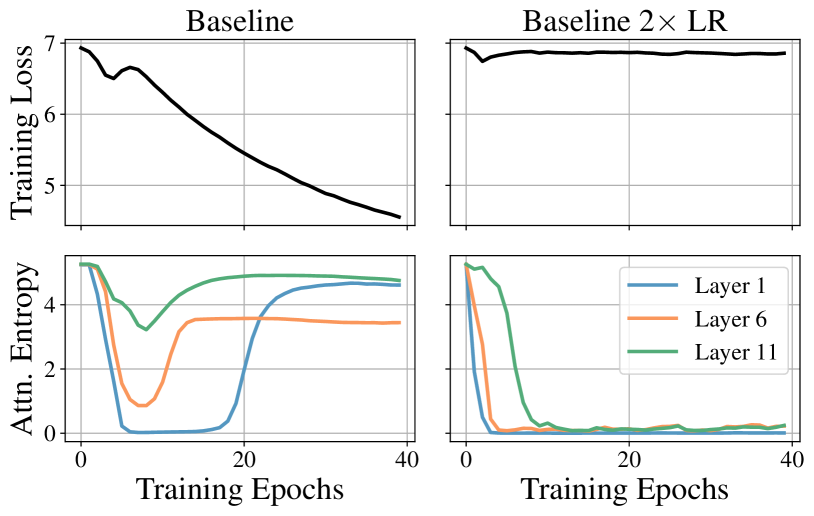
Figure 1: Transformers are sensitive to hyperparameters. Increasing the learning rate easily causes attention entropy collapse and training divergence. Left: baseline Vision Transformer with default hyperparameters from Touvron et al. (2021); right: $2\times$ learning rate ($5\times 10^{-4}\mapsto 1\times 10^{-3})$.

Figure 2: Training can become unstable due to rapid change in attention logit magnitude. We train a Vision Transformer, sharply reducing its temperature in the attention logits by $10\times$ at different intervention epochs. (Blue) Intervention during warmup – at epoch 10 – induces a sharp drop in the attention entropy of the first Transformer block. This is accompanied by an increase in the sharpness, the largest singular value of the Hessian, and exceeds the stability threshold Cohen et al. (2021) (black dashed), resulting in training instability. (Orange) Reduction after warmup – at epoch 50 – induces a less severe drop in attention entropy. The model recovers from this intervention as the sharpness does not exceed the stability threshold, although the resulting performance is lower performance than the model that did not experience any intervention (black solid).

1 Introduction

Transformers (Vaswani et al., 2017) are state-of-the-art models in many application domains. Despite their empirical success and wide adoption, great care often needs to be taken in order to achieve good training stability and convergence. In the original paper (Vaswani et al., 2017), residual connections and Layer Normalizations (LNs) (Ba et al., 2016) are extensively used for each attention and MLP block (specifically, in the post-LN fashion). There has since been various works attempting to promote better training stability and robustness. For example, the pre-LN (Radford et al., 2019) scheme has gained wide popularity, where one moves the placement of LNs to the beginning of each residual block. Others have argued that it is important to properly condition the residual connections. Bachlechner et al. (2021) proposes to initialize the residual connections to zero to promote better signal propagation. Zhang et al. (2019); Huang et al. (2020) remove LNs with carefully designed initializations.

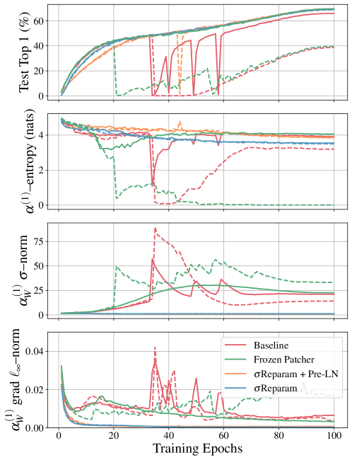
Figure 4: The best (solid line) and worst (dashed line) trials of each method from 10 trials of SimCLR for each method on ImageNet1k with 40 epochs of learning rate warmup. We show classification performance alongside relevant metrics from the first attention layer (top to bottom): attention entropy, the spectral norm of the attention weights, and the $\ell_{\infty}$–gradient norm of the attention weights. We see that the Frozen Patcher method functions as intended, regulating its gradient norm, and protecting it from the large gradient norms inducing instability in Baseline. We also observe a second form of instability during training: the growing spectral norm leads to a poorly behaved attention mechanism, entropy collapse, and a drop in performance as described in Section 3. This affects Baseline, as well as Frozen Patcher, as neither method gives specific protection against this second type of instability (solid and dashed red, and dashed green lines). Finally, we see that $\sigma$Reparam with and without pre-LN regulate both the gradient norms, as well as the spectral norms, giving defense against both types of instability.

In this work, we study the training instability of Transformers through the lens of training dynamics. We start by monitoring the entropy of the attention maps averaged over all query positions, heads and examples. We have found that the attention entropy is tightly correlated with the model’s stability and convergence. In particular, small attention entropy is often accompanied with slow convergence, fluctuations in training loss and, in the worst case, divergence. As a motivator, we plot the attention entropy curves of a highly optimized Vision Transformer (ViT) (Dosovitskiy et al., 2021; Touvron et al., 2021) in Figure 2. We observe an initial loss oscillation happening at the same time with sharp dips of the attention entropy curves. When doubling the default learning rate, all attention entropy collapses to near zero and training diverges. In addition, we show in Figures 4 and 7 two sets of experiments of baseline Transformers models with training instability occurring at the same time of entropy collapse. And more generally, similar observations can be made in a wide range of model/task settings if hyperparameters such as learning rate, warmup, initialization are not carefully tuned.

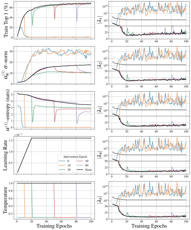
Figure 8: Training stability of a Vision Transformer under sharp reductions of its temperature by $10\times$, varying at what epoch in training the intervention occurs. We plot (left, top to bottom) training performance, the spectral norm of the first attention projection matrix, the attention entropy of the first attention block, the learning rate and the temperature, (right, top to bottom) the largest to fifth largest singular values of the Hessian by magnitude. We see that interventions in the warmup period – at epochs 10 and 20 – induce a sharp drop in the entropy $\alpha^{(1)}$ of the attention mechanism in the first Transformer block. This is accompanied by an increase in the sharpness $|\lambda_{1}|$ beyond the stability threshold Cohen et al. (2021, 2022) (black dashed), resulting in training instability. Interventions afterwards, at epochs 20, 30, 50 and 80 all induce a drop in attention entropy, but no entropy collapse. These models also recover as the sharpness does not exceed the stability threshold. We also show the performance of an unintervened Transformer (None).

To further demonstrate this connection, we modify the Transformer to have a global temperature by dividing the pre-softmax (logits) matrix of each attention mechanism by a scalar quantity whose default value is 1. Modifying the temperature gives direct control over the attention entropy, enabling the investigation of a causal connection between entropy collapse and training instability (see Figure 2 and Figures 8 and 9 in Appendix B). Here we train a ViT-B/16 on ImageNet1k. At an intervention epoch we modify the temperature from its default value to 0.1. We see that when performing this intervention during warmup, attention entropy drops to near zero and training becomes unstable. A late intervention also causes a drop in entropy and accuracy curves, however, the model is able to recover to a higher attention entropy regime, although yielding a lower accuracy than non-intervened training.

To further understand these phenomena, we computed the sharpness – the largest singular value of the Hessian (the second order derivative of the loss with respect to the model parameters), as its magnitude has implications for training stability Ghorbani et al. (2019); Yao et al. (2020); Cohen et al. (2021, 2022); Gilmer et al. (2021). When sharpness exceeds an algorithm-dependent stability threshold, training iterations diverge Cohen et al. (2021, 2022). We see that interventions inducing the largest drop in attention entropy result in the sharpness exceeding the stability threshold, whereas the later interventions do not cause the threshold to be crossed, explaining how they can recover. For details on the empirical setup and additional results see Appendix B.

The empirical correlation of entropy collapse and training instability leads to the following questions: 1) How do we prevent entropy collapse? 2) Can we improve training stability by doing so? We answer these by showing that entropy collapse can be effectively prevented by controlling the spectral norms of the query and key projections. In particular, we prove a tight lower bound on the attention entropy, which decreases exponentially fast with the growth of the spectral norm of the attention matrix logits. This bound suggests that entropy collapse can occur swiftly when letting the spectral norm of the weights increase uncontrollably. We then provide a simple fix, $\sigma$Reparam, which reparameterizes all weight matrices by sequentially applying Spectral Normalization (Miyato et al., 2018) and a learned multiplicative scalar. Intuitively, $\sigma$Reparam decouples the update of the spectral norms of weights from their dimensionality, which allows them to update smoothly and in a controlled way. Also note that $\sigma$Reparam does not change the model space, which allows one to learn an equally expressive model.

We evaluate five tasks: image classification, self-supervised learning (SSL), machine translation, automatic speech recognition (Appendix E), and language modeling (Appendix G). We highlight the empirical results as follows:

1. We show that entropy collapse is commonly observed in the baseline models of various benchmarks.

2. Image classification: $\sigma$Reparam enables a drastically simplified ViT training recipe by removing pre-LN, learning rate warmup, weight decay and not requiring adaptive optimizers. This recipe leads to equivalent (or slightly better) model performance against baseline training strategies, all the while reducing training duration by 16% .

3. Self-supervised learning: $\sigma$Reparam helps to drastically improve the stability and robustness of the SimCLR training, improving upon existing baselines.

4. Machine translation: $\sigma$Reparam allows us to stabilize very deep post-LN architectures up to 100L-100L encoder-decoder layers.

5. Speech recognition: $\sigma$Reparam allows us to improve training stability and simplify the training recipe for post-LN Transformer by removing learning rate warmup and adaptive optimization.

6. Language modeling: $\sigma$Reparam is compatible with causal Transformer architectures, and achieves results competitive with state-of-the-art without using post-LN.

2 Related Works

Transformers have relied heavily on LNs to achieve training stability. Besides the popular post-LN and pre-LN configurations, other variants have been proposed (Wang et al., 2022; Shleifer et al., 2021; Liu et al., 2020a). On the one hand, we show empirically that entropy collapse (and its accompanied training instability) happens even equipped with extensive use of normalization layers. On the other hand, $\sigma$Reparam does not rely on specific normalization layers and can even work in the absence of it, while effectively smoothing the attention entropy curves.

There have also been numerous attempts to design better Transformer initialization schemes, including Zhang et al. (2019); Huang et al. (2020); Yang et al. (2022); Bachlechner et al. (2021). While proper initializations are indeed crucial to stable and fast training, we argue that the training dynamics (affected by the optimizer and training hyperparameters) is equally important. $\sigma$Reparam in this sense is an orthogonal approach that specifically targets the entropy collapse problem, which makes it compatible with standard initialization methods and provides robust performance.

$\sigma$Reparam is a special case of weight reparameterization, which has found wide adoption in deep learning. WeightNorm (WN) (Salimans & Kingma, 2016) is a well known example of such methods, but its effectiveness in Transformers is limited. In ConvNets, simple additive weight reparameterization (Ding et al., 2021) has been demonstrated useful in speeding up training convergence. To the best of our knowledge, $\sigma$Reparam is the first simple reparameterization technique that provides competitive performance with well optimized baseline models. Normalizing weights by its spectral norm is also inspired by SpectralNorm (Miyato et al., 2018), with the key difference that SpectralNorm explicitly constrains the model’s capacity, which brings significant performance loss.

Another related line of work is the rank collapse of Transformer training, first identified by (Dong et al., 2021). Rank collapse refers to the degenerate state of attention where its output converges to a rank 1 matrix, where all tokens share the same representation. This analysis is further followed up by (Anagnostidis et al., 2022) suggesting that rank collapse causes vanishing gradient of the attention query and keys. Entropy collapse, on the other hand, characterizes a different failure pattern, where the attention matrix remains high rank, and it tends to introduce high gradient norms rather than vanishing gradients (see Figure 4).

3 Method

3.1 Attention Entropy

At the core of Transformers is dot-product attention. Let $X\in\mathbb{R}^{T\times d}$ denote an input sequence to an attention layer (we assume self-attention for simplicity of presentation), where $T,d$ are the number of tokens and the token dimension, respectively; and let $W_{K},W_{Q}\in\mathbb{R}^{d\times n_{a}},W_{V}\in\mathbb{R}^{d\times n_{v}}$ denote the key, query and value matrices. A simple attention layer then computes $\text{Att}(X)=AXW_{V}$ where $A=\psi(a),a=XW_{K}W_{Q}^{\top}X^{\top}$ and $\psi$ is the row-wise softmax function. We define the attention entropy of a row $i$ of $A$ by $\text{Ent}(A_{i})=-\sum_{j=1}^{T}A_{i,j}\log(A_{i,j})$. Let $\text{Ent}(A)=\frac{1}{T}\sum_{i=1}^{T}\text{Ent}(A_{i})$ denote the average attention entropy of $A$. Our goal is to alleviate the entropy collapse problem and achieve a smooth evolution of the attention entropy through training.

We next investigate the properties of attention entropy. We show in the next theorem that $\text{Ent}(A)$ is directly connected to the spectral norm (the largest singular value) of $W_{K}W_{Q}^{\top}$.

Theorem 3.1 (Attention entropy lower bound).

Let $\sigma=\|W_{K}W_{Q}^{\top}\|_{2}$, $\sigma_{x}=\|XX^{\top}\|_{2}$, $\bm{\sigma}=\sigma\sigma_{x}$ and $\beta=\exp\left(-\bm{\sigma}\sqrt{\tfrac{T}{T-1}}\right)$. Then it holds that:

$$\text{Ent}(A_{i}) \geq\log\left(1+(T-1)\,\beta\right)+\frac{\bm{\sigma}\sqrt{T(T-1)}\,\beta}{1+(T-1)\,\beta}.$$ (1)

Moreover, there exist inputs $X$ and weights $W_{K},W_{Q}$ for which the lower bound in Equation 1 is tight.

Therefore, for large $\sigma,T$, the minimum attainable entropy behaves like $\Omega(T\sigma e^{-\bm{\sigma}})$, hence decreasing exponentially fast with $\bm{\sigma}$. We note that the bound on the entropy in 3.1 is tight in a sense that it is achievable for some inputs $X$. Proofs for Theorem 3.1 and the following Proposition are provided in Appendix A.

Entropy collapse and training stability. Transformers are hard to train, requiring a careful tuning of a variety of hyperparameters. Notably, transformers can exhibit stages of training instability, with loss values oscillating uncontrollably, to the point of divergence. From a loss geometry perspective, we hypothesize that these regions of instability are caused when the weights enter a region of high curvature, a hypothesis supported by Chen et al. (2022), which showed that transformer models tend to converge to extremely sharp local minima. In this paper however, we step away from the loss geometry perspective and identify a novel empirical observation unique to the Transformer architecture. We observe that training instability and attention entropy collapse appear in tandem. Moreover, this observation is consistent across multiple settings and modalities (see Figures 12, 15, 7, 17 and 4). Equipped with this observation, we might ask whether preventing attention collapse might in turn prevent training instability. We highlight that the affirmative answer provided in this paper could prove extremely practical, as attention entropy is easier to compute and potentially manipulate then directly tackling the loss geometry, which typically involves computing second derivatives, as in Foret et al. (2021). We next describe out method for preventing entropy collapse through a simple reparameterization scheme.

3.2 $\sigma$Reparam

$\sigma$Reparam is a method to reparameterize the weights of a linear layer with:

$$\widehat{W}=\frac{\gamma}{\sigma(W)}W,$$ (2)

where $\sigma(W)\in\mathbb{R}$ is the spectral norm of $W$ and $\gamma\in\mathbb{R}$ is a learnable parameter, initialized to 1. In practice, $\sigma(W)$ can be computed via power iteration (Mises & Pollaczek-Geiringer, 1929) as in SpectralNorm (SN) (Miyato et al., 2018), see Algorithm 1 in Appendix C for a sketch implementation. Note that $\sigma$Reparam brings little extra overhead as the power iteration mainly consists of two matrix vector products and is only performed on the parameters rather than activations. During inference, one can compute $\widehat{W}$ once and freeze it, which has the same cost of a regular linear layer.

$\sigma$Reparam decouples the update rate of spectral norm from the dimensionality of weights. As is the case with other reparameterization techniques, $\sigma$Reparam leaves the representational capacity of the network intact, however forces a different optimization dynamic. This property makes it distinct from SN, which explicitly constrains the model space. By absorbing the spectral norm $\sigma$ into a single parameter $\gamma$, $\sigma$Reparam effectively forces the updates for $\gamma$ to be dimensionality independent. This property is in contrast to the naive parameterization, where the spectral norm of weight matrices grows rapidly for large weight matrices when equipped with adaptive optimizers. To illustrate this, we adopt common assumptions in stochastic optimization, and model the stochastic gradients at some point in the optimization by $g=\mu+\epsilon\in\mathbb{R}^{w\times w}$, where $\mu$ is the mean and $\epsilon$ is a random variable with $\mathbb{E}[\epsilon]=\mathbf{0},\mathbb{E}[\epsilon^{2}]=n^{2}\in\mathbb{R}^{w\times w}$. A typical Adam optimizer update attempts to approximate the following ideal update: $\Delta=\frac{\mathbb{E}[g]}{\sqrt{\mathbb{E}[g^{2}]}}$. The following proposition lower bounds the spectral norm of the ideal update $\sigma(\Delta)$:

Proposition 3.2.

It holds that:

$$\sigma(\Delta)\geq\sqrt{w}\sqrt{1-\frac{1}{w^{2}}\sum_{i,j=1}^{w}\frac{n_{i,j}^{2}}{\mu_{i,j}^{2}+n_{i,j}^{2}}}.$$ (3)

The noise second moment $n^{2}$ is typically in the order of $\mu^{2}$, hence Equation 3 indicates that the spectral norm of the ideal update should be large, growing linearly with $\sqrt{w}$. Moreover, for large batch sizes we would have $n^{2}\ll 1$, resulting in $\sigma(\Delta)\sim\sqrt{w}$ . While such a large spectral norm could be offset by a proper learning rate adjustment, this would be counterproductive since 1) a small learning rate typically induces inferior performance, and 2) architectures with layers of varying sizes, such as the case in Transformers, would require a per layer learning rate tuning. In contrast, $\sigma$Reparam avoids this issue since the spectral norm of each layer is controlled by a single parameter $\gamma$, hence the size of its update does not scale with $w$ and is uniform across layers. This indicates $\sigma$Reparam should provide the models of improved robustness with respect to learning rate and other related hyperparameters, by maintaining the spectral norm of the weights (and as a result the attention entropy) in a healthy regime.

Table 1: Supervised image classification on ImageNet1k. The B/L/H refer to ViT-B/16, ViT-L/16 and ViT-H/14 variants respectively. The H and L variants have a known overfitting trend on this dataset (He et al., 2022). SN corresponds to the spectral normalization baseline without the learnable scalar, while WN refers to the WeightNorm baseline. The WN configuration leads to immediate divergence without using pre-LN; we thus only report the result with WN + pre-LN.

	DeiT (B)	$\sigma$Reparam (B)	SN (B)	WN (B)	MAE (B/L/H)	$\sigma$Reparam (B/L/H)
Top-1 (%)	81.8	82.2	69.81	77.51	82.1 / 81.5 / 80.90	81.88 / 82.41 / 81.09
Training Epochs	300	300	250	250	300 / 200 / 200	250 / 300 / 170
pre-LN	Yes	No	No	Yes	Yes	No
SGD	No	No	Yes (LARS)	No	No	Yes (LARS)
Cosine Schedule	Yes	Yes	No	No	Yes	No
LR Warmup	Yes	Yes	No	No	Yes	No
Weight Decay	Yes	Yes	No	No	Yes	No

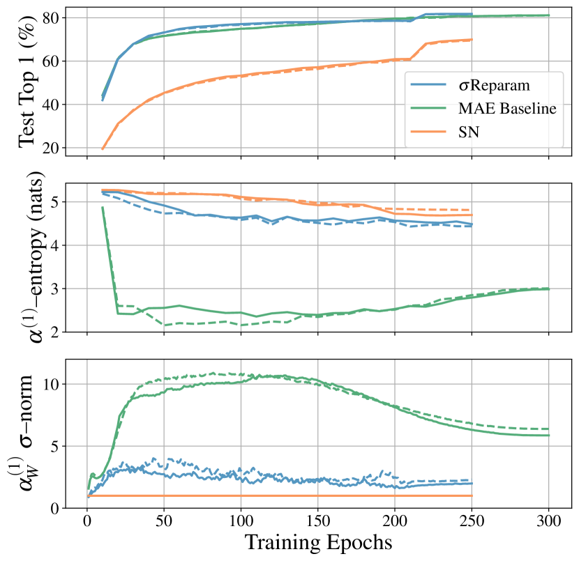
Table 2: Finetuned supervised image classification on ImageNet1k after pretraining on ImageNet21k (11M samples) or larger data. We compare $\sigma$Reparam, trained for 90 epochs against DeiT3 (Touvron et al., 2022) (trained for 90 [-90E] and 240 [-240E] epochs), an optimized finetuned CLIP (Dong et al., 2022), and a scaled supervised ViT-B trained on JFT-3B (Zhai et al., 2022). All models compared use the ViT-B/16 architecture. $\sigma$Reparam presents competitive results and sits in between the DeiT3-90E and DeiT3-240E runs, while not using pre-LN, LR warmup and only requiring a small weight-decay of $10^{-5}$.

	DeiT3-240E	DeiT3-90E	CLIP FT	ViT-B	$\sigma$Reparam
Test Top-1 (%)	86.7	85.2	86.6	86.6	85.84
EMA Top-1 (%)	-	-	-	-	85.87
Dataset size	11M	11M	400M	3B	11M
Finetuning res	384	224	384	384	384
pre-LN	Yes	Yes	Yes	Yes	No
Optimizer	LAMB	LAMB	AdamW	Adafactor	LAMB
LR Schedule	Cos	Cos	Cos	r-sqrt	step
LR Warmup	Yes	Yes	Yes	Yes	No
Weight Decay	Yes	Yes	Yes	Yes	Yes

Figure 3: ImageNet1k test performance, attention entropy, and largest singular value of attention weights of a supervised $\sigma$Reparam ViT-B/16 alongside supervised MAE ViT-B/16 and spectral normalization (SN) baselines. Best (solid line) and worst (dashed line) trials of each method are presented. The MAE ViT-B/16 presents a more constrained attention entropy in contrast to the DeiT formulation from Figure 2 due to the longer warmup, lower learning rate and stronger weight decay. While the SN baseline presents stable training, the model substantially under performs $\sigma$Reparam.

4 Experiments

4.1 Supervised Image Classification

Improved robustness. We first start from a well tuned recipe with ViT-B on ImageNet1k (Deng et al., 2009; Touvron et al., 2021), and vary its hyperparameters in the grid $\Big{[}\texttt{baseLR}\in\{5\times 10^{-4},10^{-3}\}$, $\texttt{batchSize}\in\{1024,\,2048\}$, $\texttt{warmupEpochs}\in\{0,5\}\Big{]}$. 7/8 configurations lead to divergence except for the default $\Big{[}5\times 10^{-4},$ $2048,$ $5\Big{]}$ hyperparameter. We next apply $\sigma$Reparam to all the linear layers (including the initial patch embedding), and remove all the pre-LNs instances. All configurations in the same grid search converge with an average top-1 accuracy of 81.4% ($\pm$0.52%) demonstrating improved robustness with respect to hyperparameters.

Simplified recipe. $\sigma$Reparam also enables a simplified framework for training ViT-B, ViT-L and ViT-H models, in contrast to state-of-the art ImageNet1k ViT training protocols such as the fully supervised MAE recipe (He et al., 2022) and DeiT (Touvron et al., 2021), see Table 1. In the case of ViT-B models, we are able to train for a shorter duration, remove all pre-LNs layers, remove learning rate (LR) warmup, remove cosine scheduling (requiring only a simple step schedule at 210 epochs) and use no weight decay. Furthermore, $\sigma$Reparam enables SGD training via LARS (You et al., 2017) (with momentum 0.9) – something not possible with traditional ViT training protocols (Touvron et al., 2021; He et al., 2022). These simplifications also have the added benefit of reducing GPU memory overhead. For the ViT-L model we relax the LR schedule back to cosine and slightly increase the training interval to 300 epochs. All models use FP32 precision on the attention and $\sigma$Reparam operands and keep mixed precision training for the rest of the network. The full set of hyperparameters is available in Appendix H. We note that for larger models like the ViT-L/16 and ViT-H/14 a slight weight decay cosine schedule from $0.0$ to $10^{-5}$ enables easier training.

To further understand the effect of $\sigma$Reparam, we track both the attention entropy, and the largest singular value of the attention weight matrix over the course of training. In Figure 3, $\sigma$Reparam maintains lower spectral norms for the attention weight matrices and presents a higher, but monotonically decreasing attention entropy throughout training. The benefit of such smooth and bounded attention entropy curves is reinforced by the accelerated performance observed in Test Top 1 and the 50 epoch reduction in training time for the $\sigma$Reparam ViT-B/16 shown in Figure 3.

Finally, we extend $\sigma$Reparam to a much larger 11M sample training dataset, ImageNet21k (Ridnik et al., 2021), and train a ViT-B/16. We then finetune this model with ImageNet1k and report the performance in Table 2. We observe that $\sigma$Reparam presents competitive results against ViT-B/16’s trained on drastically larger datasets such as JFT3B (Zhai et al., 2022) and the 400M sample CLIP pre-training dataset (Dong et al., 2022), all the while presenting stable training and not requiring LayerNorm or LR warmup.

4.2 Self-Supervised Training of Visual Representations

Table 3: (Top) Best SimCLR ImageNet1k trial top 1 linear probe performance training for 300 epochs. $\sigma$Reparam + pre-LN yields the highest performing run, with Frozen Patcher performing competitively. (Bottom) Configuration of the variants used in our stability analysis. The MoCo v3 weight initialization and patch initialization scheme are described in Chen et al. (2021). For full hyperparameters, see Table 6 of Section D.1.

	Baseline	Frozen Patcher	$\sigma$Reparam	$\sigma$Reparam + pre-LN
Top 1 @ 300 (ours)	72.4	74.4	73.7	74.5
Weight Init	MoCo v3	MoCo v3	trunc_norm(.02)	trunc_norm(.02)
Patcher Init	MoCo v3	MoCo v3	trunc_norm(.02)	trunc_norm(.02)
Frozen Patcher	No	Yes	No	No
$\sigma$Reparam	No	No	Yes	Yes
pre-LN	Yes	Yes	No	Yes

In computer vision, SSL has been effective in enabling efficient training on downstream tasks (Assran et al., 2022). Most of this progress has been made using convolutional architectures, while works using ViTs often require specialized training recipes (Caron et al., 2021).

Recently, it was found that ViTs suffer from training instabilities in SSL tasks (Chen et al., 2021). These instabilities can be remedied through a combination of frozen patch embedders, initialization schemes, and longer learning rate warmups; however, there is an open question whether a general solution providing stable SSL ViT training exists (Chen et al., 2021).

Here, we demonstrate that $\sigma$Reparam is a ViT SSL stabilizer. Taking SimCLR as our SSL method, we investigate four variants. Baseline and Frozen Patcher were studied in Chen et al. (2021), whereas $\sigma$Reparam and $\sigma$Reparam + pre-LN are our solution.

These methods are detailed in Table 3, and their full hyperparameters are given in Table 6 of Section D.1.

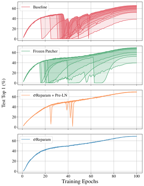
Figure 5: Linear probe performance of each of the 10 trials of SimCLR for each stabilization method. We see that $\sigma$Reparam is the most stable method. $\sigma$Reparam + pre-LN is also quite stable. In the case where it experiences instabilities, we see that it is able to recover much quicker than Baseline and Frozen Patcher. This is due to the regularization of the spectral norm which 1) prevents any arising instability pushing the model too far away from the current solution, and 2) keeps the attention mechanism useful, such that gradients are available for any required correction.

We observe two types of instability. The first, as observed in Chen et al. (2021), is induced by large gradient norms in early layers. The second, described in Section 3, relates to entropy collapse. We find that Frozen Patcher protects against the first type, but is still susceptible to the second. $\sigma$Reparam, however, can protect against both types of instability, yielding more reliable training (see Figures 5 and 4).

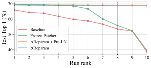
Figure 6: Linear probe performance on ImageNet1k at the end of training over 10 trials for each method. Trials are ordered by decreasing performance, with run rank 1 (10) corresponding to the best (worst) trial. Frozen Patcher and $\sigma$Reparam + pre-LN produce the best individual runs, with $\sigma$Reparam marginally lower. $\sigma$Reparam + pre-LN and $\sigma$Reparam are the methods most reliably giving good performance, with Baseline and Frozen Patcher each susceptible to at least one instability type.

As noted in Chen et al. (2021), instabilities reduce final performance. We show the instability impact on performance below. in Figure 6. The methods with the best performing individual runs are Frozen Patcher and $\sigma$Reparam + pre-LN, whereas the most stable methods are $\sigma$Reparam + pre-LN and $\sigma$Reparam.

Our main stability experiments use 40 epochs of learning rate warmup, matching the setting of Chen et al. (2021). Using $\sigma$Reparam, as in the supervised setting, gives training stability even at the lower learning rate warmup of 10 epochs. For more details, see Section D.2.

Finally, we look at the performance attainable when training for a longer duration of 300 epochs in Table 3. The best performing method run is given by $\sigma$Reparam + pre-LN, with Frozen Patcher performing almost as well, and both outperforming the reference SimCLR result (Chen et al., 2021).

Ultimately, we see while $\sigma$Reparam produces the lowest degree of instability, the best overall method for stable training of SimCLR ViTs is $\sigma$Reparam + pre-LN, producing both the highest ImageNet1k linear probe performance at 100 epochs (69.6 %) and 300 epochs (74.5 %) epochs, as well as very stable training over many trials, both at long and short learning rate warmup.

4.3 Machine Translation

Figure 7: MT training on WMT’17 for 100L-100L DeepNorm and DeepNorm with injected $\sigma$Reparam across 3 runs with different seeds: training loss (bottom), encoder self-attention entropy (top) and encoder-decoder cross-attention entropy (middle) for 95th layers. Attention entropy collapse with further model divergence is observed for DeepNorm, while $\sigma$Reparam is bounding entropy and provides stable training.

In machine translation (MT) stable training of deep encoder-decoder post-LN Transformers is an active research area (Wang et al., 2022; Liu et al., 2020a). Vanishing gradients problem has been reported by many works, leading to different solutions including rescaling residual connections: e.g., Wang et al. (2022) trained a 1000-layer Transformer by properly rescaling residual connections and initialization depending on model depth, dubbed DeepNorm. We examined attention entropy collapse for the deep Transformers in MT and found that they suffer not only from vanishing gradients but also from entropy collapse, both for vanilla post-LN and DeepNorm. By injecting $\sigma$Reparam alongside post-LN/DeepNorm, we empirically show that it is able to bound attention entropy and stabilize training without any divergent training loss growth issues. Details on experiments and all findings are in Appendix F.

Empirical setup. We use standard WMT’17 English-German benchmark with newstest2016 as a validation and newstest2017 as test sets. We consider $N$L-$N$L encoder-decoder models with $N$ encoder and $N$ decoder layers, where $N=6,18,50,100$, for both post-LN and DeepNorm configurations. For all models we report BLEU score on validation and test sets across 3 runs with different seeds.

Table 4: Results for MT on WMT’17 English-German data for post-LN, with or without additional $\sigma$Reparam, with or without residual rescaling (‘DeepNorm’ from Wang et al. (2022)). We report average BLEU score and its std across 3 runs with different seeds for a variety of encoder-decoder architectures: 6L-6L, 18L-18L, 50L-50L, and 100L-100L. ‘DV’ states for how many times a model diverges / is not training across runs. With red block we mark unstable baseline training while with blue block – training stabilized by $\sigma$Reparam.

Models	6L-6L			18L-18L			50L-50L			100L-100L
	DV	Valid BLEU	Test BLEU	DV	Valid BLEU	Test BLEU	DV	Valid BLEU	Test BLEU	DV	Valid BLEU	Test BLEU
post-LN	0/3	34.20.2	27.80.2	1/3	35.20.2	29.00.2	3/3	-	-	3/3	-	-
+ $\sigma$Reparam	0/3	34.30.3	27.80.2	0/3	35.20.2	28.70.2	0/3	34.90.3	28.50.6	3/3	-	-
DeepNorm	0/3	34.20.2	27.90.2	0/3	35.70.4	29.20.2	0/3	35.70.2	29.20.1	2/3	35.20.0	29.20.0
+ $\sigma$Reparam	0/3	34.40.4	27.70.2	0/3	35.20.2	28.60.1	0/3	34.80.4	28.30.3	0/3	34.40.1	28.00.1

Attention entropy collapse occurs in deep models. While we reproduced stable results for 6L-6L post-LN and observed nicely bounded attention entropy behaviour, for 18L-18L configurations, divergence is observed when varying the random seed. By close inspection we observe no vanishing gradients problem, but attention entropy collapse clearly occurs during training. Deeper models, namely 50L-50L and 100L-100L, are unable to train due to vanishing gradients as well as attention entropy collapse for some of the deep layers (Figure 17). For DeepNorm while we are able to reproduce results for 6L-6L, 18L-18L and 50L-50L depths observing stable training (no any models diverged and training behaved well), yet we observe instability in training of the 100L-100L model, resulting in only 1 over 3 (different seeds) successful run. By closer inspection of the training behaviour we do not see any drastic issue of vanishing gradients, however we see attention entropy collapse, see Figures 7 and 18.

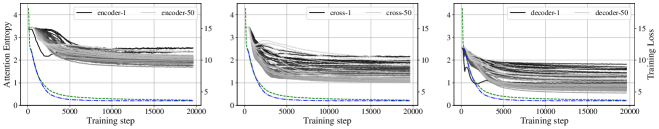
Figure 20: Attention entropy behaviour for MT models trained on WMT’17 with DeepNorm (Wang et al., 2022) (residual rescaling and post-LN) and $\sigma$Reparam together for 50L-50L (top) and 100L-100L (bottom): encoder self-attention (left), encoder-decoder cross-attention (middle) and decoder self-attention (right). We plot training (dashed, green) and validation (dot-dashed, blue) losses and attention entropy across all Transformer layers (solid): a lighter color corresponds to a deeper layer. Usage of $\sigma$Reparam allows to nicely bound attention entropy (across encoder, decoder and cross-attention) for both 50L-50L and 100L-100L and fully stabilize training (across $>10$ runs with different hyperparameters and seeds we did not observe any instability and model divergence) of DeepNorm alone for 100L-100L allowing even larger learning rate values.

$\sigma$Reparam resolves entropy collapse in deep models. To alleviate attention entropy collapse and confirm $\sigma$Reparam effectiveness for deep models we inject $\sigma$Reparam into post-LN and DeepNorm models. As a result, $\sigma$Reparam nicely bounds attention entropy for 18L-18L and 50L-50L post-LN models (Figure 19), resolving any divergence issues as well as vanishing gradients in the 50L-50L model. $\sigma$Reparam also nicely bounds attention entropy for 18L-18L, 50L-50L, 100L-100L DeepNorm models (Figure 20), resolving any divergence issues for 100L-100L, see Figure 7 (vanishing gradients are not observed as DeepNorm targets it). In terms of performance (Table 4), $\sigma$Reparam with post-LN or DeepNorm matches their baselines for 6L-6L and in the same ballpark for 18L-18L. However, $\sigma$Reparam is inferior to DeepNorm for 50L-50L and 100L-100L.

4.4 Speech Recognition and Language Modeling

We also conduct empirical analysis of speech recognition in Appendix E and observe attention entropy collapse for different configurations. $\sigma$Reparam alongside with post-LN (a) stabilizes training of post-LN (b) improves robustness with respect to hyperparameters and (c) to the best of our knowledge, for the first time allows model training without an adaptive optimizer achieving stable training and comparable performance. For language modeling, see Appendix G, $\sigma$Reparam simplifies training recipe by removing all LayerNorms and achieves comparable performance to state-of-the-art.

5 Conclusion

Transformer training stability is a well acknowledged, but still unsolved problem. This problem comes with many facets, and there are multiple necessary conditions that need to be met in order to guarantee stable and robust training. Our work identifies attention entropy collapse as a unique failure pattern that seems to be commonly observed in a wide range of settings and tasks. We also show that $\sigma$Reparam as a simple reparameterization of the weights can effectively address the entropy collapse problem, which often leads to improved training stability and robustness.

There are also limitations of our work. First of all, it is unclear if there is a causal relationship between entropy collapse and training instability of Transformers. We believe that establishing such a connection will enable a deeper understanding of the challenges of Transformer training from the optimization perspective. Second, $\sigma$Reparam, while effective, is not a panacea. In the practical sense, one might still benefit from combining $\sigma$Reparam with many other useful techniques, including initialization, feature normalization, advanced optimizers, etc. We hope that our work opens new perspectives towards inventing new design and training principles in the future.

6 Acknowledgement

We would like to thank Navdeep Jaitly, Vimal Thilak, Russ Webb for their helpful feedback and critical discussions on the experimental part of the work; Samy Bengio, Andy Keller, Russ Webb, Luca Zappella for their help throughout the process of writing this paper; Hassan Babaie, Mubarak Seyed Ibrahim, Li Li, Evan Samanas, Cindy Liu, Guillaume Seguin, Okan Akalin, and the wider Apple infrastructure team for assistance with developing scalable, fault tolerant code; and Shuming Ma for providing details on the DeepNorm reproduction steps. Names are listed in alphabetical order.

Appendix A Proof of 3.1 and 3.2

See 3.1

Proof.

Without loss of generality let $u\in\mathbb{R}^{T}$ denote the $i$’th row of $A$, $u=A_{i}$. From the assumptions it holds that $\|u\|\leq\bm{\sigma}$. Let $p=p(u)$ denote the softmax probabilities given by:

$$p_{j}=\frac{e^{u_{j}}}{Z},$$ (4)

where $Z=\sum_{k=1}^{T}e^{u_{k}}$ is the partition function. The entropy given $p(u)$ is then:

$$\text{Ent}(u)=-\sum_{j=1}^{T}\frac{e^{u_{j}}}{Z}\log\left(\frac{e^{u_{j}}}{Z}\right)=-\sum_{j=1}^{T}\frac{u_{j}e^{u_{j}}}{Z}+\log(Z).$$ (5)

We wish to solve the following minimization problem:

$$\min_{u}\text{Ent}(u)~{}~{}\text{s.t}~{}~{}\|u\|^{2}\leq\bm{\sigma}^{2},$$ (6)

Define the Lagrangian:

$$\mathcal{L}(u,\lambda)=\text{Ent}(u)+\frac{1}{2}\lambda(\|u\|^{2}-\bm{\sigma}^{2}).$$ (7)

To find all saddle points, we solve the system of equations:

$$\frac{\partial\mathcal{L}(u,\lambda)}{\partial u}=0,~{}~{}~{}\frac{\partial\mathcal{L}(u,\lambda)}{\partial\lambda}=0.$$ (8)

Giving rise to the following set of equations:

$$\forall_{1\leq k\leq T},~{}\lambda u_{k} =\sum_{j=1}^{T}\frac{e^{u_{j}}}{Z}\left[\delta_{j,k}-\frac{e^{u_{k}}}{Z}\right]\left[1+\log\left(\frac{e^{u_{j}}}{Z}\right)\right]$$ (9)

$$=p_{k}[\log(p_{k})+\text{Ent}(u)]$$ (10)

$$\|u\|^{2} =\bm{\sigma}^{2}.$$ (11)

As a first step, assume that for the minimizer $u^{\star}$ of Equation 6 there exists an index $k^{\star}$ such that $u^{\star}_{k^{\star}}=0$. Using Equation 10:

$$0 =\log(p_{k}^{\star})+\text{Ent}(u)=-\sum_{j=1}^{T}p_{j}\log\left(\frac{p_{j}}{p_{k^{\star}}}\right)=-\sum_{j=1}^{T}p_{j}\log(e^{u_{j}})=-\sum_{j=1}^{T}p_{j}u_{j}=-\mathbb{E}u.$$ (12)

From the first set of equations we arrive at the condition:

$$\forall_{u_{j_{1}}\neq 0,u_{j_{2}}\neq 0},~{}p_{j_{1}}\frac{\log(p_{j_{1}})+\text{Ent}(u)}{u_{j_{1}}} =p_{j_{2}}\frac{\log(p_{j_{2}})+\text{Ent}(u)}{u_{j_{2}}}$$ (13)

$$\longrightarrow p_{j_{1}}+\frac{\mathbb{E}u}{u_{j_{1}}} =p_{j_{2}}+\frac{\mathbb{E}u}{u_{j_{2}}}$$ (14)

$$\longrightarrow p_{j_{1}}=p_{j_{2}}.$$ (15)

This however implies that $u_{1}=u_{2}=...=u_{T}=0$, hence a contradiction to Equation 11.
Now, assuming $\forall_{k}~{}u_{k}\neq 0$, we have using Equation 10:

$$\forall_{u_{j_{1}}\neq u_{j_{2}}},~{} \frac{p_{j_{1}}}{u_{j_{1}}}[\log(p_{j_{1}})+\text{Ent}(u)]=\frac{p_{j_{2}}}{u_{j_{2}}}[\log(p_{j_{2}})+\text{Ent}(u)]$$ (16)

$$\longrightarrow e^{u_{j_{1}}}\left(1-\frac{\mathbb{E}u}{u_{j_{1}}}\right)=e^{u_{j_{2}}}\left(1-\frac{\mathbb{E}u}{u_{j_{2}}}\right).$$ (17)

We now make the following observation: we may assume a solution $u$ to Equation 6 must contain at least one negative component. To see this, consider $u$ such that $u>0$ component wise, and $\|u\|\leq\bm{\sigma}$. We can always move $u$ by some vector $v|\forall_{i,j}~{}v_{i}=v_{j}$ such that $\|u-v\|\leq\bm{\sigma}$ where $u-v$ has at least one negative component. Since all components in $v$ are equal, we have that $\text{Ent}(u)=\text{Ent}(u-v)$. Moreover, without loss of generality we may assume that $\mathbb{E}u>0$ due to the same logic.

Let $u_{j_{1}},u_{j_{2}}<0$, then according to Equation 17:

$$e^{u_{j_{1}}}\left(1-\frac{\mathbb{E}u}{u_{j_{1}}}\right)=e^{u_{j_{2}}}\left(1-\frac{\mathbb{E}u}{u_{j_{2}}}\right)>0$$ (18)

Note that $f(x)=e^{x}(1-\frac{\gamma}{x})$ is monotonously increasing in $x\in(-\infty,0)$ and $x\in[\gamma,\infty)$ for $\gamma>0$, implying that $u_{j_{1}}=u_{j_{2}}$. Similarly, if $u_{j_{1}}<0$ and $u_{j_{2}}>0$, then $e^{u_{j_{2}}}\left(1-\frac{\mathbb{E}u}{u_{j_{2}}}\right)>0$ hence $u_{j_{2}}>\mathbb{E}u_{j_{2}}$. Since $f(x)=e^{x}(1-\frac{\gamma}{x})$ is monotonous in $x$ for both $x<0$ and $x>\gamma$, we conclude that a solution $u$ must contain 2 unique values, one positive and one negative. Let the different components be $\alpha,\beta$ such that $\alpha>0,\beta<0$. A minimizer of the entropy would correspond to a $u$ with $T-1$ components equal to $\beta$, and 1 component equal to $\alpha$, such that:

$$\alpha=\bm{\sigma}\sqrt{1-\frac{1}{T}},~{}~{}~{}\beta=-\bm{\sigma}\sqrt{\frac{1}{T(T-1)}},$$ (19)

with the corresponding entropy:

$$\text{Ent}(u^{\star})=\log\left(1+(T-1)e^{-\bm{\sigma}\sqrt{\frac{T}{T-1}}}\right)+\frac{\bm{\sigma}\sqrt{T(T-1)}e^{-\bm{\sigma}\sqrt{\frac{T}{T-1}}}}{1+(T-1)e^{-\bm{\sigma}\sqrt{\frac{T}{T-1}}}}.$$ (20)

∎

See 3.2

Proof.

We have that:

$$\sigma(\Delta)\geq\frac{1}{\sqrt{w}}\sqrt{\text{Trace}(\Delta^{\top}\Delta)} =\frac{1}{\sqrt{w}}\sqrt{\sum_{i,j=1}^{w}\frac{\mu_{i,j}^{2}}{\mu_{i,j}^{2}+n_{i,j}^{2}}}=\sqrt{w}\sqrt{1-\frac{1}{w^{2}}\sum_{i,j=1}^{w}\frac{n_{i,j}^{2}}{\mu_{i,j}^{2}+n_{i,j}^{2}}}.$$ (21)

∎

Appendix B Relationship Between Entropy Collapse and Training Instability

B.1 Experimental Outline

Here we will investigate the interplay between entropy collapse and training stability by asking: would a model with stable training but not exhibiting entropy collapse have been stable if entropy collapse was induced, all other factors held constant? In do-calculus (Pearl, 2009), this roughly corresponds to checking

$$P\left(\text{stable}=\text{True}|\,\text{stable}=\text{True},\,\text{collapse}=\text{False},\,\text{do}(\text{collapse}=\text{True})\right)<1.$$

Inducing entropy collapse

Note that logits ${\bm{u}}\in\mathbb{R}^{d}$ and temperature $\tau$ give rise to the temperature normalized softmax

$$p_{i}({\bm{u}},\tau)=\frac{\exp(u_{i}/\tau)}{\sum_{j=1}^{d}\exp(u_{j}/\tau)}$$ (22)

and corresponding entropy

$$H_{p}({\bm{u}},\tau)=-\frac{1}{d}\sum_{i=1}^{d}p_{i}({\bm{u}},\tau)\,\log\,p_{i}({\bm{u}},\tau).$$ (23)

Holding ${\bm{u}}$ constant, the entropy is low when $\tau\rightarrow 0$, and is high when $\tau\rightarrow\infty$. As entropy collapse is observed in experiments when $H_{p}({\bm{u}},\tau)\rightarrow 0$, we will attempt to induce entropy collapse by sending $\tau\rightarrow\tau_{\text{target}}$, where $\tau_{\text{target}}\ll 1$.

Concretely, for a Transformer model, we normalize the logits of the attention matrix by temperature. We use the same temperature normalization for every layer, i.e. the Transformer has a global temperature. We start the temperature $\tau=1$ which corresponds to the default Transformer model without temperature normalization. At a prescribed epoch during training, we perform a temperature intervention, where we change the temperature from $\tau=1$ to a target temperature $\tau_{\text{target}}$. The transition is sharp, and happens at the start of the prescribed epoch, which we refer to as the intervention epoch.

We use the MAE ViT-B/16 recipe (see Appendix H) for these experiments, and train for a total of 100 epochs on ImageNet1k. To simplify the analysis, we only use ImageNet1k training augmentations, and use no learning rate decay schedule (i.e. the learning rate is flat after warmup).

Eigenvalues of the Hessian

As properties of the Hessian have been successfully used to gain an understanding of stability of the learning process Ghorbani et al. (2019); Yao et al. (2020); Cohen et al. (2021, 2022); Gilmer et al. (2021), we will also use them in our analysis. Specifically, we will analyze the magnitude $|\lambda_{i}|$ of the largest magnitude eigenvalues $\lambda_{i}$ of the Hessian $H$

$$H_{a,b} =\frac{\partial^{2}\mathcal{L}}{\partial\theta^{a}\partial\theta^{b}}, H \in\mathbb{R}^{P\times P}, Hv_{i} =v_{i}\lambda_{i}, ||v_{i}|| =1,$$ (24)

where $\theta^{a}$ is the $a$–th parameter, $\mathcal{L}$ is the scalar loss, $P$ is the number of model parameters, and $v_{i}$ is the normalized eigenvector corresponding to the eigenvalue $\lambda_{i}$. We take $|\lambda_{1}|>|\lambda_{2}|>\ldots>|\lambda_{P}|$, and call the largest eigenvalue $|\lambda_{1}|$ the sharpness, in line with the stability literature.

Computing and storing the Hessian explicitly is problematic, as it is $O(P^{2})$ in time and memory. Instead, noting that the Hessian Vector Product (HVP) $Hv$ for any vector $v$ can be computed using the Vector Jacobian Product (VJP) or Jacobian Vector Product (JVP), avoiding explicit computation of $H$. Treating the HVP as a linear operator then allows the use of numerical methods for computing the spectrum Yao et al. (2020); Ghorbani et al. (2019). For our iterative method we use the implementation of Lanczos from CuPy Okuta et al. (2017). We compute the 5 largest eigenvalues of $H$ using 32,768 samples from the ImageNet1k training set, and perform this computation at the end of each training epoch.

The Stability Threshold

Different optimization algorithms have a stability threshold; under a local quadratic assumption, if any Hessian eigenvalue of the loss exceeds this threshold, iterations of the optimization procedure will diverge Cohen et al. (2021, 2022). For AdamW, the stability threshold $\Gamma$ is derived in the case of a short time-horizon frozen (i.e. non-fully adaptive) approximation of AdamW, has been shown empirically as a suitable stability threshold for the full algorithm Cohen et al. (2022), and is given by

$$\Gamma=\frac{2+2\,\beta_{1}}{1-\beta_{1}}\frac{1}{\eta}=\frac{38}{\eta},$$ (25)

where $\beta_{1}=0.9$ is the Adam momentum of the gradient moving average Kingma & Ba (2015). We include this threshold in our analysis.

B.2 Results

Figure 9: Training stability of a Vision Transformer under modifications of its temperature at epoch 10 in training. We plot (left, top to bottom) training performance, the spectral norm of the first attention projection matrix, the attention entropy of the first attention block, the learning rate and the temperature, (right, top to bottom) the largest to fifth largest singular values of the Hessian by magnitude. We see that reducing the temperature to below 0.15 causes a sharp drop in the entropy $\alpha^{(1)}$ of the attention mechanism in the first Transformer block and an increase in the sharpness $|\lambda_{1}|$ beyond the stability threshold Cohen et al. (2021, 2022) (black dashed), resulting in training instability. Temperatures larger than 0.16 but lower than 1 do not induce training as they do not cross the stability threshold, although these interventions cause a moderate drop in attention entropy before recovery. We also investigated increasing the temperature, to ensure we were not just “shocking” the system, and in fact it is a drop in temperature that is particularly problematic. Setting the temperature to 100 increases the entropy as expected, but also induces a drop in performance. These models also recover as the sharpness does not exceed the stability threshold.

Appendix C Implementation of $\sigma$Reparam

To compute the spectral norm of the current matrix we use the power method as an approximation method to speed up computations. See Algorithm 1 for a sketch implementation. Note that in practice fp32 precision is typically required for numerical stability. We have experimented with various configurations applying $\sigma$Reparam to key and query weights, and/or in other parts (e.g., all other linear layers in the model). While we found that the performance is robust to the configurations, applying it to all the layers amounts to the simplest implementation and also works well in practice, e.g., allowing the removal of LN layers. $\sigma$Reparam does not bring any overhead compared to pre-LN or post-LN configurations, see Table 5.

Algorithm 1 Pseudo code of $\sigma$Reparam in a PyTorch-like style.

⬇

# Parameters. W: weight matrix, shape (d, c); gamma: the learned spectral norm, shape (1,)

# Buffers. u: shape (d,), v: shape (c,), the left and right singular vectors of W

if init: # initialize u, v as random unit vectors and gamma to 1

u = randn(d)

u = u / u.norm(dim=0)

v = randn(c)

v = v / v.norm(dim=0)

gamma = ones(1)

if training: # if in the training mode, perform one step of power iteration first

with torch.no_grad():

u = W.mv(v)

u = u / u.norm(dim=0)

v = W.T.mv(u)

v = v / v.norm(dim=0)

sigma = einsum(’d,dc,c->’, u, W, v)

W_hat = gamma / sigma * W # the effective spectral norm of W_hat would be gamma

Table 5: Time for one training step for different normalizations in different domains.

Model	ASR (ms)	MT 8L-18L (ms)
post-LN	450	1700
pre-LN	450	1800
$\sigma$Reparam	450	2200
+ post-LN	510	2300

Appendix D Self-Supervised Training of Visual Representations

D.1 Hyperparameters

Here we outline the hyperparameters of our experimental setup for SimCLR+ViT stability. For the variations, alongside their default hyperparameters see Table 6. These hyperparameters are used in all SimCLR runs unless stated otherwise.

Augmentations

We use SimCLR augmentations throughout, however, we run at half ColorJitter strength, equal to the ColorJitter strength of MoCo v3. For completeness, we provide our training augmentation here, our testing augmentation is the standard resize, center crop and normalize. Half color strength corresponds to color_jitter_strength = 0.5. Setting color_jitter_strength = 1.0 recovers the base SimCLR training augmentations.

⬇

[

transforms.RandomResizedCrop(

image_size_override, scale=crop_scale, interpolation=Image.BICUBIC

),

transforms.RandomHorizontalFlip(p=0.5),

transforms.RandomApply(

[

transforms.ColorJitter(

brightness=0.8 * color_jitter_strength,

contrast=0.8 * color_jitter_strength,

saturation=0.8 * color_jitter_strength,

hue=0.2 * color_jitter_strength,

)

],

p=0.8,

),

transforms.RandomGrayscale(p=0.2),

transforms.RandomApply([M.GaussianBlur([0.1, 2.0])], p=0.5),

transforms.ToTensor(),

IMAGENET_NORMALIZE,

]

Table 6: Default hyperparameters of the variants of SimCLR used in our stability analysis. The MoCo v3 weight initialization and patch initialization scheme are described in Chen et al. (2021). SinCos refers to stacked 2D SinCos positional encodings Vaswani et al. (2017). The table is divided vertically into hyperparameters that differ across methods (top) and hyperparameters shared across methods (bottom).

	Baseline	Frozen Patcher	$\sigma$Reparam	$\sigma$Reparam + pre-LN
$\sigma$Reparam	No	No	Yes	Yes
Frozen Patcher	No	Yes	No	No
Layer Norm	Yes	Yes	No	Yes
Patcher Init	MoCo v3	MoCo v3	trunc_norm(.02)	trunc_norm(.02)
Weight Init	MoCo v3	MoCo v3	trunc_norm(.02)	trunc_norm(.02)
Architecture	ViT-B/16	ViT-B/16	ViT-B/16	ViT-B/16
Batch Size	4096	4096	4096	4096
ColorJitter Strength	0.5	0.5	0.5	0.5
Learning Rate	$2\times 10^{-4}$	$2\times 10^{-4}$	$2\times 10^{-4}$	$2\times 10^{-4}$
Learning Rate Sched	Cosine	Cosine	Cosine	Cosine
Learning Rate Warmup	40 Epochs	40 Epochs	40 Epochs	40 Epochs
Optimizer	AdamW	AdamW	AdamW	AdamW
Positional Encoding	SinCos	SinCos	SinCos	SinCos
Weight Decay	0.1	0.1	0.1	0.1

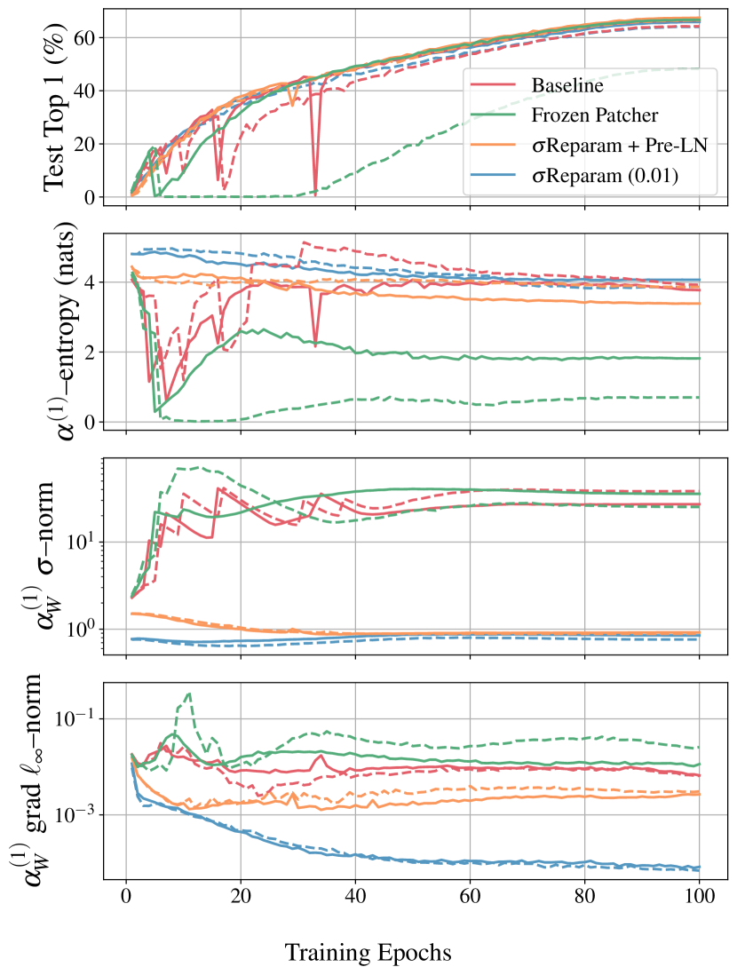
(a) Statistics of best and worst trials per method.

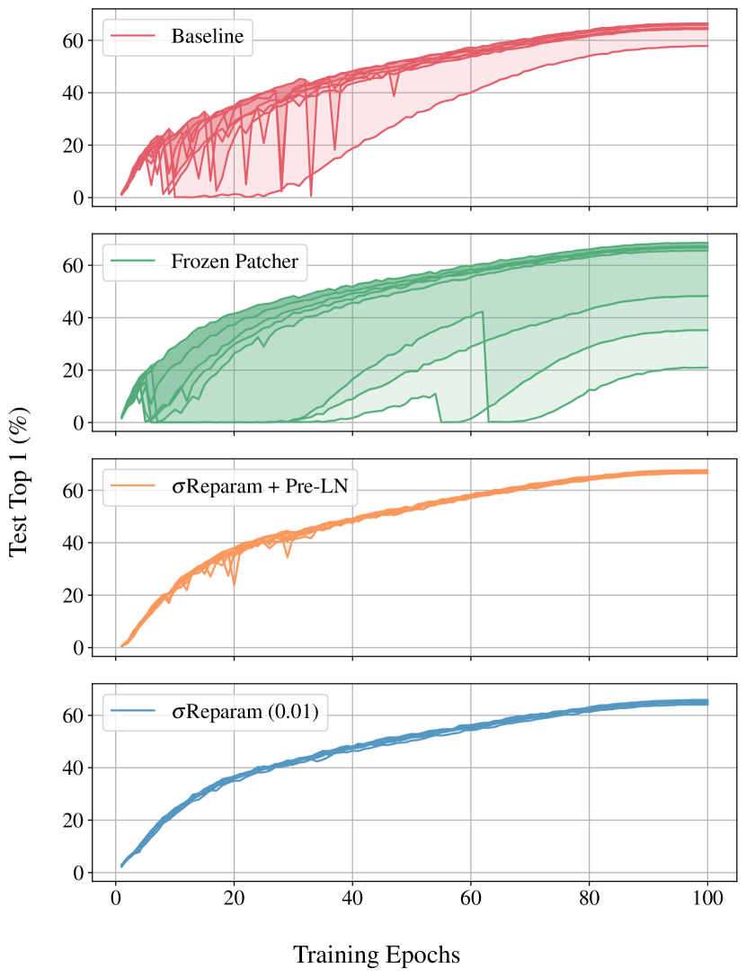
(b) Stability over 8 trials per method.

Figure 10: Eight trials of SimCLR for each method on ImageNet1k with 10 epochs of learning rate warmup. (a) Linear probe performance for the best (solid line) and worst (dashed line) trials of each method, against relevant metrics from the first attention layer (top to bottom): attention entropy, the spectral norm of the attention weights, and the $\ell_{\infty}$–gradient norm of the attention weights. Our observations are consistent with those of the longer warmup of 40 epochs investigated in Figure 5, except that here, Frozen Patcher is less able to tame early layer gradient norms than it was in the longer warmup (dashed green line). (b) Linear probe performance of every trial. Observations are again consistent with the longer warmup; $\sigma$Reparam with and without pre-LN are the most stable methods. $\sigma$Reparam (0.01) refers to a $\sigma$Reparam with an initialization scheme of trunc_normal(.01) instead of trunc_normal(.02), with the former showing some signs of instability. Understanding the source of this instability will be the subject of future work. $\sigma$Reparam + pre-LN uses the default trunc_normal(.02).

D.2 Reduced Learning Rate Warmup

In Chen et al. (2021) the authors noted that the learning rate warmup period needed extending from its typical ImageNet1k default of 10 epochs to 40 epochs, enhancing the stability of the method. We observe that using $\sigma$Reparam, either with or without pre-LN, we are able to achieve stable SimCLR+ViT training at the original warmup period of 10 epochs. As with our analysis at the longer warmup period, we also investigate the performance distribution across the trials, giving a sense of how instability impacts the final model (see Figures 10 and 11).

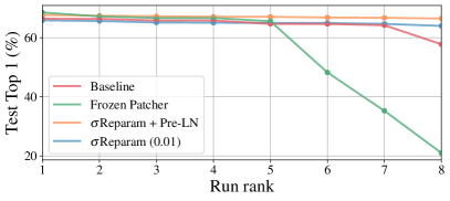
Figure 11: Linear probe performance on ImageNet1k at the end of training over 8 trials for each method. Trials are ordered by decreasing performance, with run rank 1 (8) corresponding to the best (worst) trial. Frozen Patcher produces the best individual, with all other methods marginally lower. $\sigma$Reparam + pre-LN and $\sigma$Reparam are the methods most reliably giving good performance, with Baseline and Frozen Patcher each susceptible to at least one instability type.

Appendix E Automatic Speech Recognition (ASR)

In this section we focus on empirical investigation of Transformer training stability and attention entropy collapse phenomenon for automatic speech recognition (ASR) task.

E.1 Experimental Outline

Data   All experiments are performed on the LibriSpeech dataset Panayotov et al. (2015) where audio paired with transcriptions is available. The standard LibriSpeech validation sets (dev-clean and dev-other) are used to tune all hyperparameters, as well as to select the best models. Test sets (test-clean and test-other) are used only to report final word error rate (WER) performance without an external language model. We keep the original 16kHz sampling rate and compute log-mel filterbanks with 80 coefficients for a 25ms sliding window, strided by 10ms, later normalized to zero mean and unit variance per input sequence.

Acoustic Model   We stick to a vanilla Transformer model trained with Connectionist Temporal Classification (Graves et al., 2006) loss for simplicity of analysis where only encoder is used (no decoder). We use current, to the best of our knowledge, state-of-the-art vanilla Transformer model configuration and training recipe from Likhomanenko et al. (2021a, b): the model consists of (a) 1D convolution to perform striding (kernel of 7 with stride of 3), (b) Transformer encoder with 36 layers, post-LayerNorm (post-LN), 4 heads, embedding dimension of 768 and MLP dimension of 3072, and (c) a final linear layer to map to the output number of tokens. To speed up the model training (2-3x) and decrease memory usage we are using CAPE positional embedding (Likhomanenko et al., 2021c) instead of relative one (Shaw et al., 2018): both models perform in the same ballpark.

Training   We follow a training recipe from Likhomanenko et al. (2021a, b). As they, we use SpecAugment (Park et al., 2019) which is activated right at the beginning of the training (no difference is found if it is used after 5k training steps): two frequency masks with frequency mask parameter $F=30$, ten time masks with maximum time-mask ratio $p=0.1$ and time mask parameter $T=50$ are used; time warping is not used. We also use Adagrad (Duchi et al., 2011) if not specified otherwise, and learning rate (LR) decaying by 2 each time the WER reaches a plateau on the validation set. We use dynamic batching of 240s audio per GPU and train with tensor cores fp32 on 8 Ampere A100 (40GB) GPUs for 350-500k updates. No weight decay is used. Default warmup is set to 64k and can be varied if stated so. The default LR is 0.03 and is optimized across models. We also apply gradient clipping of 1.

E.2 Training Stability, Robustness and Generalization

We start with exploring training stability of the baseline model described above using both pre-LayerNorm (pre-LN) and post-LayerNorm (post-LN) configurations trained on small-scale data, namely 100h of LibriSpeech (train-clean-100). By varying different hyperparameters, such as learning rate, warmup, and gradient clipping, post-LN models fail to train. By inspecting the gradient norms per layer and per each parameters’ matrix we find a similar vanishing gradients problem as reported, e.g., by Liu et al. (2020b, a); Wang et al. (2022) for deep Transformers ($>12$ layers) in machine translation domain. At the same time, pre-LN is stable as reported by, e.g., Nguyen & Salazar (2019); Wang et al. (2022); Liu et al. (2020a): we are able to reduce warmup from 64k to 16k, increase learning rate from 0.03 to 0.5, and obtain better results than the training setting from the post-LN baseline. However, stable training of pre-LN leads to a degradation in performance compared to post-LN in ASR, similarly as reported in the aforementioned works: validation WER is worse while training loss is lower, see top of Table 7. By varying, e.g., learning rate and warmup hyperparameters and deeper inspecting training stability of pre-LN models we observe that attention entropy is not bounded and can collapse leading to the model divergence with training loss growing, see Figure 12.

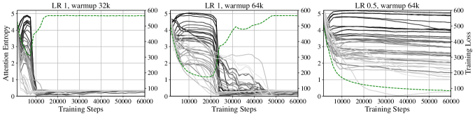
Figure 12: Attention entropy collapse is observed for pre-LN ASR models trained on 100h of LibriSpeech when hyperparameters, learning rate and warmup, are varied. For every hyperparameters configuration we plot training loss (dashed, green) and attention entropy for every of 36 layers (solid): a lighter color corresponds to a deeper layer. The right plot (LR 0.5, warmup 64k) gives stable training and the best performance while left (LR 1, warmup 64k) and middle (LR 1 and warmup 32k) have attention entropy collapse phenomenon.

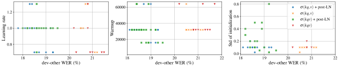
Figure 13: Robustness of $\sigma$Reparam with respect to different hyperparameters for ASR models trained on 100h of LibriSpeech: learning rate (left), warmup (middle), and initialization std value (right). We report word error rate (WER, x-axis) on the validation dev-other set.

As discussed above in Section 3, we now investigate how $\sigma$Reparam affects the training stability and controls the attention entropy bound. First, by removing all LayerNorms (pre-LN or post-LN) and switching to $\sigma$Reparam for all linear layers in Transformer blocks and in the final linear layer, we observe (a) stable training similar to pre-LN with no vanishing gradients issue; (b) accepting a wider range of hyperparameters (Figure 13) than pre-LN; (c) no attention entropy collapse phenomenon. While $\sigma$Reparam significantly outperforms a pre-LN model with the baseline hyperparameters used for post-LN, it performs worse than an optimized version of a pre-LN model as well as an unstable post-LN model (see top of Table 7). However, combining $\sigma$Reparam with post-LN brings two worlds together: stable training similar to pre-LN and generalization similar to post-LN. In summary, $\sigma$Reparam with post-LN achieves (a) similar performance on the validation and test sets and lower training loss (Table 7); (b) no vanishing gradients are observed as for post-LN; (c) the model accepts a wide range of hyperparameters (Figure 13) compared to unstable post-LN and stable pre-LN.

To demonstrate the necessity of $\sigma$Reparam in the form presented in Section 3, we compare it with spectral normalization (SN) where $\gamma$ is set to 1 and is not learnable, and WeightNorm (Salimans & Kingma, 2016) baselines. Both SN and WN perform poorly compared to $\sigma$Reparam (with or without post-LN), see Table 7.

Table 7: Results for ASR training on 100h of LibriSpeech with $\sigma$Reparam and/or different normalizations: post-layer (post-LN), pre-layer (pre-LN), spectral (SN), weight (WN). We report training loss and word error rate (WER, % $\downarrow$) for the best models for each configuration: with warmup and Adagrad optimizer (top), and with no warmup and LARS optimizer (bottom). DV states for model divergence. For bottom part: $\sigma$Reparam performs reparametrization for joint matrix for key, queries and values in self-attention, and we are not able to train SN with post-LN configuration.

	post-LN	pre-LN	pre-LN	SN	SN	WN	WN	$\sigma$Reparam	$\sigma$Reparam
		(same)	(optimized)		+post-LN		+post-LN		+post-LN
Training loss	37.7	35.3	37.2	160.4	120.3	35.6	35.4	37.5	34.9
dev-clean WER	5.9	6.9	6.2	42.6	20.3	7.0	6.3	6.4	6.1
dev-other WER	17.7	21.3	19.1	62.9	42.7	22.3	19.4	20.5	17.8
test-clean WER	6.2	7.1	6.3	42.4	20.4	7.3	6.7	6.8	6.4
test-other WER	17.8	21.6	19.3	63.6	43.6	22.6	19.5	21.0	18.0
Training loss	64.5	-	29.4	160.0	DV	59.1	63.2	51.1	34.2
dev-clean WER	8.1	-	5.9	49.8	DV	8.3	7.1	7.2	5.8
dev-other WER	25.0	-	18.9	69.6	DV	25.9	22.0	22.8	18.1
test-clean WER	8.6	-	6.4	49.4	DV	8.7	7.5	7.5	6.2
test-other WER	25.6	-	19.2	70.9	DV	26.4	22.1	23.2	18.7

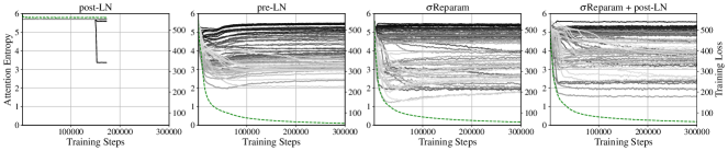
Figure 14: Deep, 72 layers, ASR models trained on 100h of LibriSpeech with different normalizations (from left to right): with post-LN, pre-LN, $\sigma$Reparam, $\sigma$Reparam with post-LN. We plot training loss (dashed, green) and attention entropy for every of 72 layers (solid): a lighter color corresponds to a deeper layer.

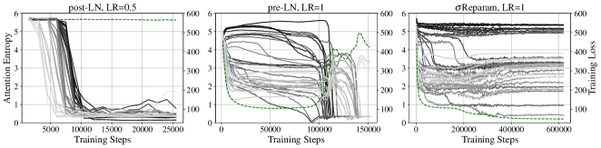
Figure 15: ASR models trained on 100h of LibriSpeech with different normalizations (from left to right: with post-LN, pre-LN, $\sigma$Reparam) and LARS optimizer. We plot training loss (dashed, green) and attention entropy for every of 36 layers (solid): a lighter color corresponds to a deeper layer. Post-LN and pre-LN models have attention entropy collapse when learning rate is increased to 0.5 and 1, correspondingly, while $\sigma$Reparam has no issue.

We further investigate training behaviour if we increase the model depth by 2x resulting in 72 encoder layers. In such setting we are unable to train a post-LN model (vanishing gradients are observed) while pre-LN, $\sigma$Reparam and $\sigma$Reparam with post-LN are training out of the box and have bounded attention entropy throughout the training with no vanishing gradients problem, see Figure 14.

E.3 Training with SGD

Vanishing gradients and unbalanced gradients can be one of the reasons why the standard SGD fails in training Transformers, especially for deeper architectures, and one needs adaptive optimizers. E.g., Li et al. (2022) report also another issue with SGD – ability for generalization, and propose Transformer components modification to improve generalization with SGD training.

To confirm prior findings, we first experiment with baseline models, pre-LN and post-LN, and SGD optimizer. While post-LN is not training, a pre-LN model can be trained but has a poor generalization. The same holds for $\sigma$Reparam and $\sigma$Reparam with post-LN: the gradient magnitude between the first and last layers can differ not drastically as in post-LN, but generalization is still poor. Similarly to vision experiments, we switch to the LARS (You et al., 2017) (with momentum 0.9) optimizer which normalizes gradients by their magnitudes and thus provides balanced gradients. By carefully tuning only the learning rate from 0.1 to 1.5 (the rest stays the same as for the adaptive optimizer except warmup which is set to 0k) we are able to train pre-LN and post-LN, see bottom of Table 7.

In our experiments post-LN is more unstable (many learning rates are diverging or not training) and gives significantly worse results than pre-LN. Furthermore, pre-LN is still behind the baseline that uses an adaptive optimizer. However, if we switch to $\sigma$Reparam (key, queries and values are represented as one matrix) we observe stable training with respect to learning rate changes, and combined together with post-LN it achieves similar performance to the best results from top of Table 7 while keeping the training loss low. To the best of our knowledge, this is the first ASR Transformer model trained without an adaptive optimizer achieving stable training and comparable performance. Regarding attention entropy collapse, we observe it with LARS training also, see Figure 15: $\sigma$Reparam controls the bound resulting in wider range of accepted hyperparameters for stable training (models can be trained with learning rate up to 1, while pre-LN and post-LN result in model divergence).

E.4 Hyperparameters

We present hyperparameters for our ASR experiments on 100h of LibriSpeech in Table 8.

Table 8: Hyperparameters comparison for ASR training on 100h of LibriSpeech for models from Table 7.

	post-LN	pre-LN	$\sigma$Reparam	$\sigma$Reparam + post-LN
dev-clean	5.9	6.2	6.4	6.1
dev-other	17.7	19.1	20.5	17.8
Weight Init	uniform(.036)	uniform(.036)	trunc_normal(.1)	trunc_normal(.1)
$\sigma$Reparam	No	No	Yes	Yes
LayerNorm	Yes	Yes	No	Yes
Base LR	0.03	0.5	1	1
Optimizer	Adagrad
LR schedule	step(330k, 0.5)
Batch size	240s x 8
Weight decay	none
Warmup steps	64k
Training steps	500k
Dropout	0.3
Stoch. Depth	0.3
SpecAugment	$F=30$, $T=50$, $p=0.1$, $fmask=2$, $tmask=10$
Grad. clip	1
dev-clean	8.1	5.9	7.2	5.8
dev-other	25	18.9	22.8	18.1
Weight Init	uniform(.036)	uniform(.036)	trunc_normal(.1)	trunc_normal(.1)
$\sigma$Reparam	No	No	Yes	Yes
LayerNorm	Yes	Yes	No	Yes
Base LR	0.1	0.5	1	0.3
Optimizer	LARS
Momentum	0.9
LR schedule	step(300k, 0.5)
Batch size	240s x 8
Weight decay	none
Warmup steps	0k
Training steps	500k
Dropout	0.3
Stoch. Depth	0.3
SpecAugment	$F=30$, $T=50$, $p=0.1$, $fmask=2$, $tmask=10$
Grad. clip	1

E.5 Large-Scale Experiments: 1k Hours of LibriSpeech

We also evaluate $\sigma$Reparam for large-scale data: for further experiments we take all $\sim$1k hours of LibriSpeech as the training data. We consider again the Adagrad optimizer with two schedules on learning rate: cosine (with 1 phase of 500k iterations) and step-wise decaying as before for train-clean-100 experiments. We use exactly the same architecture and hyperparameters as for small-scale experiments from top of Table 8 except dropout and layer drop which are decreased to 0.1 to decrease model regularization effect. For all models we tune only the learning rate. As before, spectral reparametrization of keys and queries is done separately from values. We also use the learning rate on gamma to be twice bigger than the main learning rate. Similarly to small-scale experiments, training on LibriSpeech shows (see Table 9) that $\sigma$Reparam accompanied with post-LN can match the post-LN baseline, while having robustness to the hyperparameter changes (e.g. it allows larger learning rate values without any stability issues).

Table 9: Results for ASR training on full LibriSpeech with $\sigma$Reparam and/or different normalizations: post-layer (post-LN), pre-layer (pre-LN). We report word error rate (WER, % $\downarrow$) for the best models for each configuration: with step-wise (top) and cosine (bottom) learning rate schedules.

	post-LN	post-LN	pre-LN	pre-LN	$\sigma$Reparam	$\sigma$Reparam
	(Likhomanenko et al., 2021b)		(same)	(optimized)		+post-LN
dev-clean WER	2.6	2.6	2.9	2.6	2.7	2.8
dev-other WER	7.0	6.9	7.7	6.8	7.2	7.1
test-clean WER	2.7	2.7	3.0	2.8	2.9	2.9
test-other WER	6.9	6.9	7.8	6.8	7.3	7.0
dev-clean WER	-	2.6	2.6	-	2.8	2.7
dev-other WER	-	7.1	6.9	-	7.6	7.3
test-clean WER	-	2.9	2.8	-	3.0	2.9
test-other WER	-	7.2	7.0	-	7.7	7.2

Appendix F Machine Translation (MT)

In this section we focus on empirical investigation of training stability and attention entropy collapse in deep Transformers for machine translation (MT) with an encoder-decoder architecture. We track attention entropy for the encoder self-attention, the decoder cross-attention and the encoder-decoder self-attention separately to study the entropy collapse phenomenon. The goal of this section is to understand how varying the model depth for the well-established recipes affects the training stability.

F.1 Experimental Outline

We build our experiments on top of the open-sourced code and baseline recipes provided by Wang et al. (2022). We follow their instructions and hyperparameters given in Wang et al. (2022).

Data   Following Wang et al. (2022) we perform all experiments on standard WMT’17 English-German benchmark: we use all provided training data for English-German pair, newstest2016 set as a validation set and newstest2017 as a test set for final evaluation purpose only. We use Fairseq (Ott et al., 2019) script to preprocess data: it uses Byte Pair Encoding (BPE) vocabulary jointly for source and target language resulting in 41k subword tokens.

Models   We consider both regular and deep configurations for a vanilla encoder-decoder Transformer model with $N$ encoder and $N$ decoder layers where $N$ is taken as 6 (6L-6L), 18 (18L-18L), 50 (50L-50L), and 100 (100L-100L). Every Transformer layer in each configuration has an embedding dimension of 512, MLP dim of 2048, and 8 heads. Sinusoidal absolute positional embedding (Vaswani et al., 2017) is used for both encoder and decoder.

Training    We strictly follow the same training recipe from Wang et al. (2022) (without using back-translation or other domain-specific augmentations) with detailed hyperparameters in Table 10. All models are trained on 8 GPUs of A100 80GB with mixed precision computations and dynamic batching resulting in total batch size of 524288 tokens: for each architecture we pack maximum tokens per GPU and use gradient accumulation (4 for 6L-6L and 18L-18L, 8 for 50L-50L and 16 for 100L-100L).

Table 10: Hyperparameters comparison for MT training on WMT’17 for models from Table 11.

	pre-LN/post-LN/DeepNorm	$\sigma$Reparam + post-LN	$\sigma$Reparam + deepnorm
Weight Init	Fairseq	trunc_normal(.1/.01)	trunc_normal(.1/.01)
$\sigma$Reparam	No	Yes	Yes
LayerNorm	Yes	Yes	Yes
Base LR	1.4e-3	4.5e-3	4.5e-3
Optimizer	Adam
LR schedule	inverse sqrt
Batch size	4096 tokens x 8 GPUs x 16 gradient accumulation
Weight decay	0.0001
Warmup steps	4k
Warmup init LR	1e-7
Training steps	100k
Dropout	0.4
Grad. clip	0
Adam $\epsilon$	1e-8
Adam $\beta$	(0.9, 0.98)
Label smoothing	0.1

Evaluation   As it is not specified in Wang et al. (2022) how the best checkpoint is selected on the validation set, we decided to stick to simple rule: checkpoint with best perplexity on the validation set is selected and further evaluated on both validation and test sets for BLEU score computation which is reported throughout the paper. BLEU is computed by in-built BLEU scripts of Fairseq with the beam size of 5. As reported in prior works we also observe a strong correlation between perplexity and BLEU score: improved perplexity leads to better BLEU score. However BLEU scores on validation and test sets are less correlated and high variation is observed. For that reason we often perform 3 runs with different seeds to estimate standard deviation (std) of the BLEU score.

F.2 Training Stability of Deep Models

Table 11: Results for MT on WMT’17 English-German data for post-LN, with or without additional $\sigma$Reparam, with or without residual rescaling (‘DeepNorm’ from Wang et al. (2022)). We report average BLEU score and its std across 3 runs with different seeds for a variety of encoder-decoder architectures: 6L-6L, 18L-18L, 50L-50L, and 100L-100L. ‘DV’ states for how many times a model diverges / is not training across runs. With red block we mark unstable baseline training while with blue block – training stabilized by $\sigma$Reparam.

Models	6L-6L			18L-18L			50L-50L			100L-100L
	DV	Valid BLEU	Test BLEU	DV	Valid BLEU	Test BLEU	DV	Valid BLEU	Test BLEU	DV	Valid BLEU	Test BLEU
pre-LN	0/3	34.20.1	27.40.1	0/3	35.30.1	28.80.1	0/3	34.90.1	28.50.1	0/3	34.70.1	28.30.1
post-LN	0/3	34.20.2	27.80.2	1/3	35.20.2	29.00.2	3/3	-	-	3/3	-	-
+ $\sigma$Reparam	0/3	34.30.3	27.80.2	0/3	35.20.2	28.70.2	0/3	34.90.3	28.50.6	3/3	-	-
DeepNorm	0/3	34.20.2	27.90.2	0/3	35.70.4	29.20.2	0/3	35.70.2	29.20.1	2/3	35.20.0	29.20.0
+ $\sigma$Reparam	0/3	34.40.4	27.70.2	0/3	35.20.2	28.60.1	0/3	34.80.4	28.30.3	0/3	34.40.1	28.00.1

We start with exploring training stability of the baseline model described in Wang et al. (2022) with pre-LayerNorm (pre-LN) and post-LayerNorm (post-LN) across different depths (all hyperparameters stay the same except depth is varied). Note that post-LN is a popular design choice for MT tasks due to its good generalization properties.

For pre-LN models, we reproduced stable results and convergence, however the BLEU score we get is better (Table 11) than reported by Wang et al. (2022). We also observed the same trend of decreasing model performance with increasing the model depth. Attention entropy is nicely bounded across all depths similarly to ASR, see Figure 16.

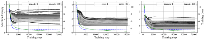
Figure 16: Attention entropy behaviour for MT models trained on WMT’17 with pre-LN for 18L-18L (top) and 100L-100L (bottom): encoder self-attention (left), encoder-decoder cross-attention (middle) and decoder self-attention (right). We plot training (dashed, green) and validation (dot-dashed, blue) losses and attention entropy across all Transformer layers (solid): a lighter color corresponds to a deeper layer. Both deep and shallow pre-LN models have nicely bounded attention entropy and no instability issues are observed across runs with different seeds.

For post-LN models, we reproduced stable results for 6L-6L depth and observe nicely bounded attention entropy behaviour. However for 18L-18L configurations, divergence is observed when varying the random seed. By close inspection we observe no vanishing gradients problem while attention entropy collapse clearly occurs during training (compare top and middle in Figure 17) in the encoder attention and the encoder-decoder cross-attention. Deeper models, namely 50L-50L and 100L-100L, are unable to train and we observe the same vanishing gradients problem as reported by Wang et al. (2022); Liu et al. (2020a) as well as attention entropy collapse for some of the deep layers across the board, see bottom plot in Figure 17.

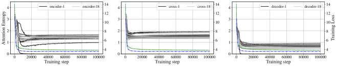
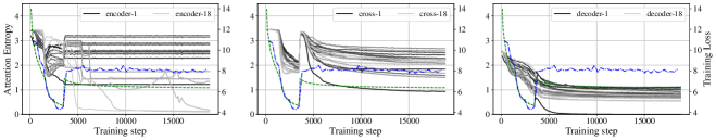
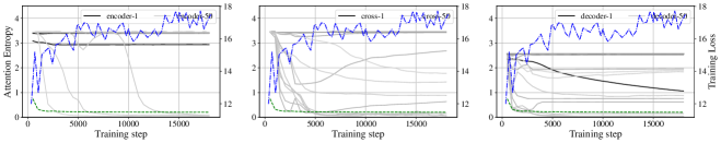
Figure 17: Attention entropy behaviour for MT models trained on WMT’17 with post-LN for 18L-18L (top, middle) with two seeds and 50L-50L (bottom): encoder self-attention (left), encoder-decoder cross-attention (middle) and decoder self-attention (right). We plot training (dashed, green) and validation (dot-dashed, blue) losses and attention entropy across all Transformer layers (solid): a lighter color corresponds to a deeper layer. While 6L-6L (not shown in Figure) has stable training, deeper models experience different issues in training: 18L-18L can be stable (top) or can diverge with attention entropy collapse phenomenon (middle) for the same hyperparameters but different seed, while 50L-50L has vanishing gradients and layers are not training resulting in constant attention entropy.

Wang et al. (2022); Liu et al. (2020a) are recent works that proposed to rescale residual connections. To stabilize training and resolve vanishing gradients problem in deep post-LN models to preserve post-LN generalization properties. We focus in this paper on Wang et al. (2022), DeepNorm, solution (it uses post-LN and rescale residual connections depending on the initial model depth) as they reported ability to train up to 1000-depth Transformer models. We are able to reproduce DeepNorm results for 6L-6L, 18L-18L and 50L-50L depths observing stable training (no any models diverged and training went nicely). However we see no performance gain of a 50L-50L depth model over a 18L-18L model. Furthermore, we observe instability in training of the 100L-100L model resulting in only 1 successful run among 3 (only seed is varied) while 2 others are diverging after some time (training loss is growing). By close inspection of the training behaviour we do not see any drastic issue of vanishing gradients, however we see the attention entropy collapse happening, see Figure 18. First of all, attention entropy is not bounded for DeepNorm even in 18L-18L and 50L-50L similarly to what we observed in post-LN models. Also a tiny attention entropy collapse happens in 50L-50L (see top plot in Figure 18) though it does not lead to any divergence. Second, attention entropy collapse is clearly pronounced for 100L-100L models (second, third, and forth rows of Figure 18) leading to 2/3 seeds divergence and one with worse performance than 50L-50L models. Finally, it is interesting to note that attention entropy collapse in 100L-100L can happen for different layers, first and / or last, and with different regimes for the encoder/decoder self-attention and the encoder-decoder cross-attention.

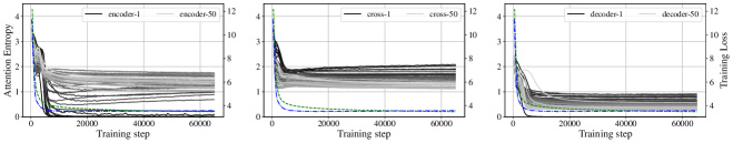
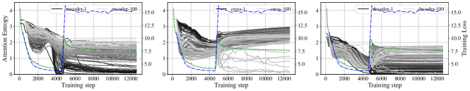
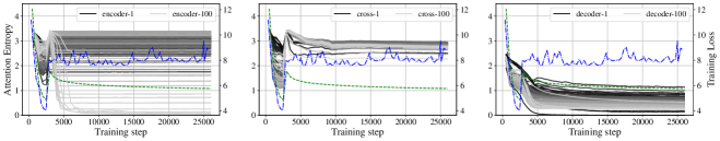
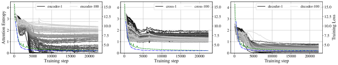
Figure 18: Attention entropy behaviour for MT models trained on WMT’17 with DeepNorm (Wang et al., 2022) (residual rescaling and post-LN) for 50L-50L (row 1) and 100L-100L with three seeds (2-4 rows): encoder self-attention (left), encoder-decoder cross-attention (middle) and decoder self-attention (right). We plot training (dashed, green) and validation (dot-dashed, blue) losses and attention entropy across all Transformer layers (solid): a lighter color corresponds to a deeper layer. While DeepNorm solves vanishing gradient problem for deep models we observe attention entropy collapse phenomenon in both 50L-50L and 100L-100L models. While the 50L-50L model can recover from attention entropy collapse (happens in encoder layers) and nicely converge, 100L-100L suffers from it and can diverge. While Wang et al. (2022) reported stable training for 100L-100L we are unable to reproduce their results and observe 2/3 runs with different seeds (the rest of hyperparameters are the same as reported in the paper) diverge with attention entropy collapse.

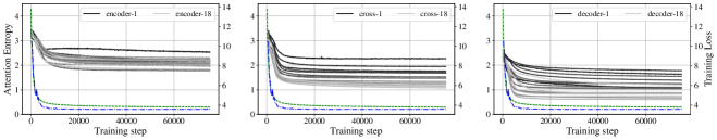
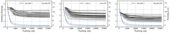
Figure 19: Attention entropy behaviour for MT models trained on WMT’17 with post-LN and $\sigma$Reparam together for 18L-18L (top) and 50L-50L (bottom): encoder self-attention (left), encoder-decoder cross-attention (middle) and decoder self-attention (right). We plot training (dashed, green) and validation (dot-dashed, blue) losses and attention entropy across all Transformer layers (solid): a lighter color corresponds to a deeper layer. While 18L-18L is unstable for post-LN models (see top and middle in Figure 17), adding $\sigma$Reparam nicely bounds attention entropy and stabilize training across different seeds and hyperparameters (we did not observe any instability or model divergence for $>10$ runs) allowing training with larger learning rates. While 50L-50L experiences vanishing gradients problem for post-LN models (see bottom in Figure 17), adding $\sigma$Reparam balances gradients across layers and nicely bounds attention entropy: training is stable across different seeds and hyperparameters accepting larger learning rates.

All models performance on validation and test sets across depths as well as the number of successful runs are reported in Table 11.

F.3 $\sigma$Reparam for Deep Models

We now experiment with injection of $\sigma$Reparam into post-LN and DeepNorm models to alleviate attention entropy collapse and confirm $\sigma$Reparam effectiveness for deep models. $\sigma$Reparam is used for every linear layer in the encoder and decoder Transformer blocks alongside with post-LN. With DeepNorm we also apply its rescaling of initialization and residual connections.

$\sigma$Reparam nicely bounds attention entropy for 18L-18L and 50L-50L post-LN models, resolving any divergence issues as well as vanishing gradient in the 50L-50L model, see Figure 19. However, 100L-100L is still experiencing a vanishing gradient problem and only careful initialization of std for $\sigma$Reparam can resolve it: for that reason we report that model training is not stable. In terms of performance, $\sigma$Reparam with post-LN matches post-LN for 6L-6L, in the same ballpark for 18L-18L and performs the same as 18L-18L for 50L-50L. Note, that we did not do any hyperparameters search except tuning learning rate as $\sigma$Reparam has different learning rate scales.

$\sigma$Reparam also nicely bounds attention entropy for 18L-18L, 50L-50L, 100L-100L DeepNorm models, resolving any divergence issues for 100L-100L (vanishing gradient is not observed as DeepNorm targets it), see Figure 19. In terms of performance $\sigma$Reparam with DeepNorm matches DeepNorm for 6L-6L, in the same ballpark as DeepNorm for 18L-18L and inferior to DeepNorm for 50L-50L and 100L-100L.

Appendix G Language Modeling (LM)

As we discussed above encoder Transformer for vision and speech domains and encoder-decoder for machine translation, in this section we focus on the pure decoder architecture in language model task to verify if $\sigma$Reparam is effective for stable training and can simplify a training recipe there too.

G.1 Experimental Outline

We use the WikiText-103 language model (LM) benchmark, which consists of 103M tokens sampled from English Wikipedia (Merity et al., 2017). Our baseline is a highly optimized Transformer (Baevski & Auli, 2019) with 32 layers, 8 heads, 128 head dimensions, 1024 model dimensions, 4096 fully connected dimensions and post-LayerNorm (post-LN). The word embedding and softmax matrices are tied (Press & Wolf, 2017). We partition the training data into non-overlapping blocks of 512 contiguous tokens and train the model to autoregressively predict each token (Baevski & Auli, 2019). Validation and test perplexity is measured by predicting the last 256 words out of the input of 512 consecutive words to avoid evaluating tokens in the beginning with limited context (early token curse, Press et al., 2021). We integrate $\sigma$Reparam implementation into the open-sourced code and recipe for the baseline. All models are trained in full precision on 8 GPUs of A100 40GB.

G.2 Results

We do not experience training instability with the baseline Transformer, likely because the masked attention in autoregressive models makes entropy collapse less likely to occur. This is consistent and in line with observations in machine translation where entropy collapse is observed in the encoder and cross-attention. Nonetheless, we experimented with $\sigma$Reparam to test its generality on a different modality/problem. We apply $\sigma$Reparam to all linear layers of the Transformer while removing all post-LNs, and search for learning rate in a grid [1, 1.5, 2, 2.5] and weight decay in the grid [1e-3, 1e-4, 0]. All other hyperparameters are kept the same as the baseline, including Nesterov SGD optimizer. The results are shown in Table 12. We see that even in the absence of LayerNorm, $\sigma$Reparam shows strong performance in convergence and validation/test performance. With a mild weight decay, $\sigma$Reparam also outperforms the baseline wrt the validation/test PPL. In summary, while there is no observed entropy collapse in language model training, $\sigma$Reparam can simplify a training recipe by removing all post-LNs.

Table 12: WikiText-103 language modeling results in perplexity.

Model	PPL$\downarrow$
	train	valid	test
$\sigma$Reparam w/ weight decay	16.5	17.9	18.6
$\sigma$Reparam w/o weight decay	12.9	18.5	19.3
post-LN Baevski & Auli (2019)	15.4	18.1	18.7

Appendix H Hyperparameters for Supervised Vision

As mentioned in Section 4.1 we compare $\sigma$Reparam against DeiT (Touvron et al., 2021) and MAE (He et al., 2022) supervised training recipes for vision Transformers. In Table 13 we highlight the differences between DeiT, MAE supervised and $\sigma$Reparam. $\sigma$Reparam presents a simplified and stable training objective for ViT-B variants. In Table 14 we present the same comparing the ViT-L variants. There is no exact 1:1 comparison for a ViT-L with the DeiT training framework so we only compare against the MAE supervised model.

Table 13: Training hyperparameters comparison for supervised ViT-B/16.

	DeiT	MAE	$\sigma$Reparam
Top-1	81.8%	82.1%	81.88%
EMA Top-1	-	82.3%	82.37%
Weight Init	trunc_normal(.02)	trunc_normal(.02)	trunc_normal(.02)
Patcher Init	trunc_normal(.02)	trunc_normal(.02)	trunc_normal(.02)
$\sigma$Reparam	No	No	Yes
Layer Norm	Yes	Yes	No
Optimizer	AdamW($\beta_{1}$=0.9, $\beta_{2}$=0.95)	AdamW($\beta_{1}$=0.9, $\beta_{2}$=0.95)	LARS(mom=0.9)
Base LR	$5\times 10^{-4}$	$1\times 10^{-4}$	0.1
LR schedule	cosine	cosine	step(210, 0.1)
Batch size	1024	4096	4096
Weight decay	0.05	0.3	0.0
Warmup epochs	5	20	0
Training epochs	300	300	250
Label smoothing	0.1	0.1	0.1
Stoch. Depth	0.1	0.1	0.1
Repeated Aug.	2	2	2
RandAug	9/0.5	9/0.5	9/0.5
Mixup prob.	0.8	0.8	0.8
Cutmix prob.	1.0	1.0	1.0
Erasing prob.	0.25	0.25	0.25

Table 14: Training hyperparameters comparison for supervised ViT-L/16.

	MAE	$\sigma$Reparam
Top-1	81.5%	82.41%
EMA Top-1	82.6%	82.48%
Weight Init	trunc_normal(.02)	trunc_normal(.01)
Patcher Init	trunc_normal(.02)	trunc_normal(.0025)
$\sigma$Reparam	No	Yes
Layer Norm	Yes	No
Optimizer	AdamW($\beta_{1}$=0.9, $\beta_{2}$=0.95)	LARS(mom=0.9)
Base LR	$1\times 10^{-4}$	0.15
LR schedule	cosine	cosine
Batch size	4096	4096
Weight decay	0.3	0.0
Warmup epochs	20	0
Training epochs	300	300
Label smoothing	0.1	0.1
Stoch. Depth	0.2	0.2
Repeated Aug.	2	2
RandAug	9/0.5	9/0.5
Mixup prob.	0.8	0.8
Cutmix prob.	1.0	1.0
Erasing prob.	0.25	0.25

Appendix I Ablations

Initialization for $\sigma$Reparam

First, we found that it is better to initialize $\gamma$ as 1 and not compute it from the initialized kernel as there could be different values for spectral norm depending on the initialization of the kernel. In this case we observed values greater than 1 for the spectral norm which cause divergence / no training. We compared different initializations for the kernel and we did not see any differences in initialization (e.g. uniform, normal). The only factor that influences training behavior is the standard deviation (std) of the initialization pdf, which also influences effective learning rate. In speech recognition we found that training is robust with respect to changes of std (Figure 13), however larger std performs better and sweet spot is 0.2-0.3. In machine translation models are also robust to the choice of std, however some architectures perform better with std of 0.01 while others with 0.1 std. In language modeling we observed robust performance with respect to initialization, and we use the default initialization from the Transformer baseline for all experiments.

In vision we initialize the $\sigma$Reparam $\gamma$ term using the first singular value, computed with the SVD at weight initialization. We then use one power iteration for all further updates. We provide weight and patcher initializations for the ViT-B/16 in Table 13 and the ViT-L/16 and ViT-H/14 in Table 14.

Separate $\sigma$Reparam for key, queries and values

We found that they behave more or less similar while separate normalization allows to achieve lower training loss due to larger capacity ability which provides potential to scale. However, for ASR training with LARS it is better to have joint reparametrization to achieve stable training and comparable results with adaptive optimizers, see Section E.3.

Appendix J Discussion

We believe that our experiments have covered representative domains, architectures and training losses for typical Transformer applications. The key factors that affect training stability are the initial token embedding layer (where for vision and speech tasks they are based on convolution projections, and for MT and language modeling are with word embeddings), topology of architecture (encoder mode for vision and speech, encoder-decoder for MT and decoder for language modeling), and the training loss (cross-entropy loss, contrastive and CTC loss). While each of these design choices may bring their own challenges for training, we show that entropy collapse is a common symptom accompanying instability and $\sigma$Reparam is a general fix compatible with all settings.

Appendix K Contributions

All authors contributed into writing the manuscript, designing experiments and discussion of all results at every stage of the project.

Attention Entropy Collapse Observations

All initial experiments and findings of the attention entropy collapse phenomenon for ViT models on ImageNet are done by Shuangfei Zhai. Preliminary theoretical analysis and proposal to use $\sigma$Reparam as a solution is also done by Shuangfei Zhai.

Theory

All theoretical results, Appendix A, are done by Etai Littwin. Review of proofs is done by Tatiana Likhomanenko.

Causality Analysis

Simulated case-control study investigation and all related experimental work done by Dan Busbridge. Tatiana Likhomanenko, Etai Littwin, Jason Ramapuram, Russ Webb and Shuangfei Zhai helped with designing the experimental setting for intervention methodology.

Supervised Learning in Vision

Shuangfei Zhai conducted the initial $\sigma$Reparam vision experiments with DeiT and made the initial observations of relaxing / removing weight decay from $\sigma$Reparam. Jason Ramapuram scaled and conducted the remaining supervised vision experiments and analysis (including the MAE, weight-norm and spectral-norm baselines) over ImageNet1k (Table 1) and Imagenet21k (Table 2) and enabled the drastically simplified $\sigma$Reparam vision transformer recipe from Table 1. This simplified $\sigma$Reparam recipe enables SGD (LARS) training over fewer epochs and completely removes {weight-decay, pre-LN layers, LR warmup and the LR cosine schedule}.

Self-Supervised Learning in Vision

Known issues with SimCLR (Chen et al., 2020) stability that were observed in Chen et al. (2021) pointed out by Vimal Thilak. All investigations, experiments and related analysis done by Dan Busbridge.

Automatic Speech Recognition

All speech recognition experiments are done by Tatiana Likhomanenko. Shuangfei Zhai and Jason Ramapuram advised to have also large scale results.

Machine Translation

Initial implementation and experiments of $\sigma$Reparam applicability to MT were done on WMT’14 by Jiatao Gu. Later, Tatiana Likhomanenko pushed to investigate deep transformer models and their stability. Jason Ramapuram pointed to the deepnorm (Wang et al., 2022) results to probe for entropy collapse phenomenon. All later experiments, Section 4.3 and Appendix F, with deep transformers and deepnorm are done by Tatiana Likhomanenko.

Language Modeling

Initial implementation and preliminary results on applicability of $\sigma$Reparam to the language modeling, Appendix G, are done by Yizhe Zhang with help from Jiatao Gu. Shuangfei Zhai contributed to the experiments and obtained the final results.

Implementation Details and Ablations

Investigation into how initialization influences $\sigma$Reparam is done in parallel in different domains and experiments by Jason Ramapuram, Shuangfei Zhai and Tatiana Likhomanenko. Investigation of different variants (with stop gradient, with different matrices) of $\sigma$Reparam was done by Shuangfei Zhai, Tatiana Likhomanenko and Jason Ramapuram. Investigation of full precision training vs mixed precision training was done by Tatiana Likhomanenko, Dan Busbridge and Jason Ramapuram.

Implementation is done in 2 frameworks (PyTorch and Jax) and in 5 codebases. The initial implementation of $\sigma$Reparam module is done in PyTorch by Shuangfei Zhai, with further reimplementation in Jax by Tatiana Likhomanenko. Later the implementation was integrated and adopted into other baseline toolboxes by Jason Ramapuram, Dan Busbridge, Yizhe Zhang, Tatiana Likhomanenko and Jiatao Gu.

References

- Anagnostidis et al. (2022) Sotiris Anagnostidis, Luca Biggio, Lorenzo Noci, Antonio Orvieto, Sidak Pal Singh, and Aurelien Lucchi. Signal propagation in transformers: Theoretical perspectives and the role of rank collapse. In Alice H. Oh, Alekh Agarwal, Danielle Belgrave, and Kyunghyun Cho (eds.), Advances in Neural Information Processing Systems, 2022. URL https://openreview.net/forum?id=FxVH7iToXS.
- Assran et al. (2022) Mahmoud Assran, Mathilde Caron, Ishan Misra, Piotr Bojanowski, Florian Bordes, Pascal Vincent, Armand Joulin, Mike Rabbat, and Nicolas Ballas. Masked siamese networks for label-efficient learning. In Computer Vision–ECCV 2022: 17th European Conference, Tel Aviv, Israel, October 23–27, 2022, Proceedings, Part XXXI, pp. 456–473. Springer, 2022.
- Ba et al. (2016) Jimmy Lei Ba, Jamie Ryan Kiros, and Geoffrey E Hinton. Layer normalization. arXiv preprint arXiv:1607.06450, 2016.
- Bachlechner et al. (2021) Thomas Bachlechner, Bodhisattwa Prasad Majumder, Henry Mao, Gary Cottrell, and Julian McAuley. Rezero is all you need: Fast convergence at large depth. In Uncertainty in Artificial Intelligence, pp. 1352–1361. PMLR, 2021.
- Baevski & Auli (2019) Alexei Baevski and Michael Auli. Adaptive input representations for neural language modeling. In International Conference on Learning Representations, 2019. URL https://openreview.net/forum?id=ByxZX20qFQ.
- Caron et al. (2021) Mathilde Caron, Hugo Touvron, Ishan Misra, Hervé Jégou, Julien Mairal, Piotr Bojanowski, and Armand Joulin. Emerging properties in self-supervised vision transformers. In Proceedings of the IEEE/CVF international conference on computer vision, pp. 9650–9660, 2021.
- Chen et al. (2020) Ting Chen, Simon Kornblith, Mohammad Norouzi, and Geoffrey Hinton. A simple framework for contrastive learning of visual representations. In International conference on machine learning, pp. 1597–1607. PMLR, 2020.
- Chen et al. (2022) Xiangning Chen, Cho-Jui Hsieh, and Boqing Gong. When vision transformers outperform resnets without pre-training or strong data augmentations. In International Conference on Learning Representations, 2022. URL https://openreview.net/forum?id=LtKcMgGOeLt.
- Chen et al. (2021) Xinlei Chen, Saining Xie, and Kaiming He. An empirical study of training self-supervised vision transformers. In Proceedings of the IEEE/CVF International Conference on Computer Vision, pp. 9640–9649, 2021.
- Cohen et al. (2021) Jeremy Cohen, Simran Kaur, Yuanzhi Li, J Zico Kolter, and Ameet Talwalkar. Gradient descent on neural networks typically occurs at the edge of stability. In International Conference on Learning Representations, 2021. URL https://openreview.net/forum?id=jh-rTtvkGeM.
- Cohen et al. (2022) Jeremy M Cohen, Behrooz Ghorbani, Shankar Krishnan, Naman Agarwal, Sourabh Medapati, Michal Badura, Daniel Suo, David Cardoze, Zachary Nado, George E Dahl, et al. Adaptive gradient methods at the edge of stability. arXiv preprint arXiv:2207.14484, 2022.
- Deng et al. (2009) Jia Deng, Wei Dong, Richard Socher, Li-Jia Li, Kai Li, and Li Fei-Fei. Imagenet: A large-scale hierarchical image database. In 2009 IEEE conference on computer vision and pattern recognition, pp. 248–255. Ieee, 2009.
- Ding et al. (2021) Xiaohan Ding, Xiangyu Zhang, Ningning Ma, Jungong Han, Guiguang Ding, and Jian Sun. Repvgg: Making vgg-style convnets great again. In Proceedings of the IEEE/CVF Conference on Computer Vision and Pattern Recognition, pp. 13733–13742, 2021.
- Dong et al. (2022) Xiaoyi Dong, Jianmin Bao, Ting Zhang, Dongdong Chen, Shuyang Gu, Weiming Zhang, Lu Yuan, Dong Chen, Fang Wen, and Nenghai Yu. Clip itself is a strong fine-tuner: Achieving 85.7% and 88.0% top-1 accuracy with vit-b and vit-l on imagenet. arXiv preprint arXiv:2212.06138, 2022.
- Dong et al. (2021) Yihe Dong, Jean-Baptiste Cordonnier, and Andreas Loukas. Attention is not all you need: Pure attention loses rank doubly exponentially with depth. In International Conference on Machine Learning, pp. 2793–2803. PMLR, 2021.
- Dosovitskiy et al. (2021) Alexey Dosovitskiy, Lucas Beyer, Alexander Kolesnikov, Dirk Weissenborn, Xiaohua Zhai, Thomas Unterthiner, Mostafa Dehghani, Matthias Minderer, Georg Heigold, Sylvain Gelly, Jakob Uszkoreit, and Neil Houlsby. An image is worth 16x16 words: Transformers for image recognition at scale. In International Conference on Learning Representations, 2021. URL https://openreview.net/forum?id=YicbFdNTTy.
- Duchi et al. (2011) John Duchi, Elad Hazan, and Yoram Singer. Adaptive subgradient methods for online learning and stochastic optimization. Journal of machine learning research, 12(Jul):2121–2159, 2011.
- Foret et al. (2021) Pierre Foret, Ariel Kleiner, Hossein Mobahi, and Behnam Neyshabur. Sharpness-aware minimization for efficiently improving generalization. In International Conference on Learning Representations, 2021. URL https://openreview.net/forum?id=6Tm1mposlrM.
- Ghorbani et al. (2019) Behrooz Ghorbani, Shankar Krishnan, and Ying Xiao. An investigation into neural net optimization via hessian eigenvalue density. In International Conference on Machine Learning, pp. 2232–2241. PMLR, 2019.
- Gilmer et al. (2021) Justin Gilmer, Behrooz Ghorbani, Ankush Garg, Sneha Kudugunta, Behnam Neyshabur, David Cardoze, George Dahl, Zachary Nado, and Orhan Firat. A loss curvature perspective on training instability in deep learning. arXiv preprint arXiv:2110.04369, 2021.
- Graves et al. (2006) Alex Graves, Santiago Fernández, Faustino Gomez, and Jürgen Schmidhuber. Connectionist temporal classification: labelling unsegmented sequence data with recurrent neural networks. In Proceedings of the 23rd international conference on Machine learning, pp. 369–376, 2006.
- He et al. (2022) Kaiming He, Xinlei Chen, Saining Xie, Yanghao Li, Piotr Dollár, and Ross Girshick. Masked autoencoders are scalable vision learners. In Proceedings of the IEEE/CVF Conference on Computer Vision and Pattern Recognition, pp. 16000–16009, 2022.
- Huang et al. (2020) Xiao Shi Huang, Felipe Perez, Jimmy Ba, and Maksims Volkovs. Improving transformer optimization through better initialization. In International Conference on Machine Learning, pp. 4475–4483. PMLR, 2020.
- Kingma & Ba (2015) Diederik P. Kingma and Jimmy Ba. Adam: A method for stochastic optimization. In Yoshua Bengio and Yann LeCun (eds.), 3rd International Conference on Learning Representations, ICLR 2015, San Diego, CA, USA, May 7-9, 2015, Conference Track Proceedings, 2015.
- Li et al. (2022) Zhiyuan Li, Srinadh Bhojanapalli, Manzil Zaheer, Sashank Reddi, and Sanjiv Kumar. Robust training of neural networks using scale invariant architectures. In International Conference on Machine Learning, pp. 12656–12684. PMLR, 2022.