Static Neutron Stars Perspective of Quadratic and Induced Inflationary Attractor Scalar-tensor Theories

Abstract

This study focuses on the static neutron star perspective for two types of cosmological inflationary attractor theories, namely the induced inflationary attractors and the quadratic inflationary attractors. The two cosmological models can be discriminated cosmologically, since one of the two does not provide a viable inflationary phenomenology, thus in this paper we investigate the predictions of these theories for static neutron stars, mainly focusing on the mass and radii of neutron stars. We aim to demonstrate that although the models have different inflationary phenomenology, the neutron star phenomenology predictions of the two models are quite similar. We solve numerically the Tolman-Oppenheimer-Volkoff equations in the Einstein frame using a powerful double shooting numerical technique, and after deriving the mass-radius graphs for three types of polytropic equations of state, we derive the Jordan frame mass and radii. With regard the equations of state we use polytropic equation of state with the small density part being either the WFF1, the APR or the intermediate stiffness equation of state SLy. The results of our models will be confronted with quite stringent recently developed constraints on the radius of neutron stars with specific mass. As we show, the only equation of state which provides results compatible with the constraints is the SLy, for both the quadratic and induced inflation attractors. Thus nowadays, scalar-tensor descriptions of neutron stars are quite scrutinized due to the growing number of constraining observations, which eventually may also constrain theories of inflation.

Introduction

The current and future status of theoretical cosmology and astrophysics is updated day by day, since astrophysical and cosmological observations are offered in high frequency. For astrophysics, the starting point of profound importance was the kilonova merging event known as GW170817 TheLIGOScientific:2017qsa ; Abbott:2020khf in which a direct observation of gravitational waves was first recorded. After that event, neutron stars (for reviews and textbooks see Haensel:2007yy ; Friedman:2013xza ; Baym:2017whm ; Lattimer:2004pg ; Olmo:2019flu ) and other astrophysical compact objects enjoy an elevated scientific role. Specifically, neutron stars are at the crossroads of many scientific eras, like nuclear theory Lattimer:2012nd ; Steiner:2011ft ; Horowitz:2005zb ; Watanabe:2000rj ; Shen:1998gq ; Xu:2009vi ; Hebeler:2013nza ; Mendoza-Temis:2014mja ; Ho:2014pta ; Kanakis-Pegios:2020kzp ; Tsaloukidis:2022rus , high energy physics Buschmann:2019pfp ; Safdi:2018oeu ; Hook:2018iia ; Edwards:2020afl ; Nurmi:2021xds , modified gravity Astashenok:2020qds ; Astashenok:2021peo ; Capozziello:2015yza ; Astashenok:2014nua ; Astashenok:2014pua ; Astashenok:2013vza ; Arapoglu:2010rz ; Panotopoulos:2021sbf ; Lobato:2020fxt ; Numajiri:2021nsc and astrophysics Altiparmak:2022bke ; Bauswein:2020kor ; Vretinaris:2019spn ; Bauswein:2020aag ; Bauswein:2017vtn ; Most:2018hfd ; Rezzolla:2017aly ; Nathanail:2021tay ; Koppel:2019pys ; Raaijmakers:2021uju ; Most:2020exl ; Ecker:2022dlg ; Jiang:2022tps . The role of modified gravity in neutron star physics is still questioned and under investigation. To date, the need of modified gravity descriptions for the large scale structure of our Universe seems rather compelling, since dark energy cannot be described in a consistent way by the use of General Relativity and scalar fields solely. To date, many works have been devoted on the physics of neutron stars in the context of modified gravity Astashenok:2014nua ; Astashenok:2014pua and its scalar-tensor counterpart theories Pani:2014jra ; Staykov:2014mwa ; Horbatsch:2015bua ; Silva:2014fca ; Doneva:2013qva ; Xu:2020vbs ; Salgado:1998sg ; Shibata:2013pra ; Arapoglu:2019mun ; Ramazanoglu:2016kul ; AltahaMotahar:2019ekm ; Chew:2019lsa ; Blazquez-Salcedo:2020ibb ; Motahar:2017blm ; Odintsov:2021qbq ; Odintsov:2021nqa ; Oikonomou:2021iid ; Pretel:2022rwx ; Pretel:2022plg ; Cuzinatto:2016ehv . In scalar-tensor theories, there exists a subclass of inflationary phenomenological models, which have the spectacular property of being inflationary attractors in the Einstein frame alpha0 ; alpha1 ; alpha2 ; alpha3 ; alpha4 ; alpha5 ; alpha6 ; alpha7 ; alpha7a ; alpha8 ; alpha9 ; alpha10 ; alpha11 ; alpha12 ; alpha13 ; alpha14 ; alpha15 ; alpha16 ; alpha17 ; alpha18 ; alpha19 ; alpha20 ; alpha21 ; alpha22 ; alpha23 ; alpha24 ; alpha25 ; alpha26 ; alpha27 ; alpha28 ; alpha29 ; alpha30 ; alpha31 ; alpha32 ; alpha33 ; alpha34 ; alpha35 ; alpha36 ; alpha37 . Specifically, distinct theories in the Jordan frame where the scalar field is non-minimally coupled to gravity, lead to Einstein frame counterpart theories which have the same inflationary observational indices, namely the same expressions for the spectral index of the primordial scalar curvature perturbations and the same tensor-to-scalar ratio. Most of the distinct attractor models are compatible with the Planck data Akrami:2018odb , thus most of these are cosmologically viable theories. In this work we shall be interested in two types of distinct cosmological attractors, the quadratic attractors and the induced inflation attractors, see alpha0 for a description of both the models. These two models correspond to different limiting cases of the coupling of the scalar field to gravity in the Jordan frame. We are interested in examining the implications of such attractor potentials on static neutron stars. After describing in brief the essential cosmological features of the two distinct attractors in the Jordan and Einstein frames, we shall derive the Einstein frame Tolman-Oppenheimer-Volkoff, which we shall solve numerically using a powerful double shooting method in order to obtain optimal initial conditions at the center of the star. The numerical method is a python 3 LSODA integrator technique which relies on double shooting for the central values of the scalar field and the metric function niksterg . The integration shall be performed for three distinct piecewise polytropic Read:2008iy ; Read:2009yp equations of state, the low density part of which shall be the Wiringa-Fiks-Fabrocini (WFF1 hereafter) Wiringa:1988tp , the Skyrme-Lyon (SLy hereafter) Douchin:2001sv , or the Akmal-Pandharipande-Ravenhall (APR hereafter) equation of state Akmal:1998cf . The numerical analysis will yield the Einstein frame radii and Arnowitt-Deser-Misner (ADM) masses Arnowitt:1960zzc of neutron stars, so by using appropriate formulas we derive the Jordan frame masses and radii. For all the cases studied we will confront the outcomes with stringent observations and constraints of specific mass neutron stars radii. We shall consider three types of constraints, developed in Refs. Altiparmak:2022bke ; Raaijmakers:2021uju ; Bauswein:2017vtn . As we show, the constraints eliminate completely the APR and WFF1 descriptions of neutron stars, and only the SLy equation of state satisfies all the constraints. This work is aligned with the new physics era discipline, where constraints on astrophysical objects may affect to some extent cosmological theories. In our case, both the inflationary attractors can describe static neutron stars consistently, however only when the matter is described by an intermediate stiffness equation of state. This is contrary to previous works, where the inflationary attractors could provide a viable description of neutron stars for all the equations of state we discuss in this paper, see for example Odintsov:2021qbq ; Odintsov:2021nqa ; Oikonomou:2021iid .

I Induced and Quadratic Inflationary Attractors and their Inflationary Phenomenology

The quadratic and induced inflationary attractors belong to a much more general class of cosmological inflationary attractors alpha0 ; alpha1 ; alpha2 ; alpha3 ; alpha4 ; alpha5 ; alpha6 ; alpha7 ; alpha7a ; alpha8 ; alpha9 ; alpha10 ; alpha11 ; alpha12 ; alpha13 ; alpha14 ; alpha15 ; alpha16 ; alpha17 ; alpha18 ; alpha19 ; alpha20 ; alpha21 ; alpha22 ; alpha23 ; alpha24 ; alpha25 ; alpha26 ; alpha27 ; alpha28 ; alpha29 ; alpha30 ; alpha31 ; alpha32 ; alpha33 ; alpha34 ; alpha35 ; alpha36 ; alpha37 , and constitute basically two different non-minimal coupling limits of the same Jordan frame non-minimally coupled scalar-tensor theory. Specifically, the gravitational action of the common Jordan frame non-minimal coupled theory is,

$$\mathcal{S}_{J}=\int d^{4}x\sqrt{-g}\Big{[}\Omega(\phi)R-\frac{1}{2}g^{\mu\nu}\partial_{\mu}\phi\partial_{\nu}\phi-U(\phi)\Big{]}+S_{m}(g_{\mu\nu},\psi_{m})\,,$$ (1)

where $\psi_{m}$ denotes the perfect matter fluids in the Jordan frame, which have pressure $P$ and energy density $\epsilon$, and $g$ is the determinant of the Jordan frame metric $g_{\mu\nu}$. Note that for the inflationary models which shall be considered in this work, the kinetic term of the scalar field has a canonical minimal coupling and appears as $-\frac{\omega(\phi)}{2}g^{\mu\nu}\partial_{\mu}\phi\partial_{\nu}\phi$ and not as $-\frac{1}{2}g^{\mu\nu}\partial_{\mu}\phi\partial_{\nu}\phi$. Also in the case at hand the non-minimal coupling function in the Jordan frame $\Omega(\phi)$ and the scalar potential $U(\phi)$ has the following form alpha0 ,

$$\Omega(\phi)=\left(1+\xi f(\phi)\right),\,\,\,U(\phi)=M_{p}^{4}\lambda\left(\Omega(\phi)-1\right)^{2}\,,$$ (2)

where $M_{p}=\frac{1}{\sqrt{8\pi G}}$ is the reduced Planck mass and $G$ is Newton’s gravitational constant. The parameters $\lambda$ and $\xi$ are dimensionless in natural units, and also the same applies for the non-minimal coupling function $f(\phi)$. Also we shall refer to the parameter $\xi$ as the non-minimal coupling hereafter. The induced and quadratic inflationary attractors correspond to different limits of the non-minimal coupling $\xi$, namely the strong coupling limit $\xi\gg 1$ and the weak coupling limit $\xi\ll 1$ respectively. Let us consider the essential inflationary features of the induced inflationary attractors, so the strong coupling limit of the initial theory. In this case, the non-minimal coupling function $\Omega(\phi)$ and the potential take the form,

$$\Omega(\phi)=\xi f(\phi),\,\,\,U(\phi)=\lambda M_{p}^{4}\xi^{2}f(\phi)^{2}\,.$$ (3)

We can obtain the Einstein frame theory which has the inflationary attractor property by performing an appropriate conformal transformation Kaiser:1994vs ; valerio ,

$$\tilde{g}_{\mu\nu}=\frac{M_{p}^{2}}{2}\Omega^{2}g_{\mu\nu}\,,$$ (4)

with the Einstein frame metric being $\tilde{g}_{\mu\nu}$, and the “tilde” will indicate the Einstein frame quantities hereafter. The minimally coupled Einstein frame canonical scalar theory action reads,

$$\mathcal{S}_{E}=\int d^{4}x\sqrt{-\tilde{g}}\Big{[}\frac{M_{p}^{2}}{2}\tilde{R}-\frac{1}{2}\tilde{g}^{\mu\nu}\tilde{\partial}_{\mu}\varphi\tilde{\partial}_{\nu}\varphi-V(\varphi)\Big{]}+S_{m}(\Omega^{-2}\frac{2}{M_{p}^{2}}\tilde{g}_{\mu\nu},\psi_{m})\,,$$ (5)

and the Einstein frame scalar potential of the canonical scalar field $\varphi$, namely $V(\varphi)$ takes the following form,

$$V(\varphi)=V_{s}\left(1-e^{-\sqrt{\frac{2}{3}}\frac{\varphi}{M_{p}}}\right)^{2}\,,$$ (6)

where $V_{s}=\frac{M_{p}^{4}\lambda}{\xi^{2}}$, and also in terms of the canonical scalar field, the non-minimal coupling function $\Omega(\varphi)$ takes the form,

$$\Omega(\varphi)=e^{\sqrt{\frac{2}{3}}\frac{\varphi}{M_{p}}}\,.$$ (7)

Also note that the matter fluids in the Einstein frame are not perfect fluids, since their energy-momentum tensor satisfies the following continuity equation,

$$\tilde{\partial}^{\mu}\tilde{T}_{\mu\nu}=-\frac{d}{d\varphi}[\ln\Omega]\tilde{T}\tilde{\partial}_{\nu}\phi\,.$$ (8)

The Einstein frame amplitude $\Delta_{s}^{2}$ of the canonical scalar field scalar perturbations,

$$\Delta_{s}^{2}=\frac{1}{24\pi^{2}}\frac{V(\varphi_{f})}{M_{p}^{4}}\frac{1}{\epsilon(\varphi_{f})}\,,$$ (9)

is constrained to be Akrami:2018odb ,

$$\Delta_{s}^{2}=2.2\times 10^{-9}\,,$$ (10)

where $\varphi_{f}$ is the value of the scalar field at the end of the inflationary era. Thus the parameter $V_{s}$ is constrained to be,

$$V_{s}\sim 9.6\times 10^{-11}\,M_{p}^{4}\,.$$ (11)

Hence the induced inflation parameters $\lambda$ and $\xi$ can be chosen in such a way so that $\frac{\lambda}{\xi^{2}}\sim 10^{-11}$, so a large $\xi\sim 10^{5}$ and a $\lambda\sim 1$ can sufficiently produce a viable inflationary era. For the induced inflationary attractors case, the spectral index of the primordial scalar curvature perturbations $n_{s}$ and the ratio of the tensor perturbations over scalar perturbations in terms of the $e$-foldings number $N$ take the form,

$$n_{s}=1-\frac{2}{N}\,,\,\,\,r=\frac{12}{N^{2}}\,.$$ (12)

Apparently, the phenomenology of the induced inflationary scenario is identical to the Starobinsky $R^{2}$ model. In fact, even the potential (7) is identical to the Starobinsky model, and this justifies the terminology attractors for the induced inflation Jordan frame theories. Note that the whole analysis is performed without even defining the form of the function $f(\phi)$ in the Jordan frame. An arbitrary $f(\phi)$ can lead to the same Einstein frame theory, and this justifies the terminology inflationary attractors. The Einstein frame theory and the corresponding phenomenology constitutes the inflationary attractor theory, regardless the exact functional form of the Jordan frame function $f(\phi)$. Notice that, by conformal invariance, the Jordan frame theory and the Einstein frame ones should produce the same inflationary phenomenology. Hence, the induced inflationary theory in the Einstein frame has the following final form,

$$\mathcal{S}_{E}=\int d^{4}x\sqrt{-\tilde{g}}\Big{[}\frac{M_{p}^{2}}{2}\tilde{R}-\frac{1}{2}\tilde{g}^{\mu\nu}\tilde{\partial}_{\mu}\varphi\tilde{\partial}_{\nu}\varphi-V_{s}\left(1-e^{-\sqrt{\frac{2}{3}}\frac{\varphi}{M_{p}}}\right)^{2}\Big{]}\,,$$ (13)

which is identical with the Starobinsky model in the Einstein frame.

At this point let us discuss an important issue. The inflationary attractor models are basically non-minimally coupled scalar field theories in the Jordan frame which yield in most cases an identical phenomenology in the Einstein frame. For example in the present case, the induced inflation attractors in the Einstein frame yield an inflationary phenomenology which is identical to the Starobinsky model in the Einstein frame. Thus these two attractors are indistinguishable when the cosmic microwave background inflationary modes are probed. These models provide a viable phenomenology and always lead to the same spectral index and tensor-to-scalar ratio which do not depend on the specific free parameters of the models, see for example Eq. (12). However, the parameters of each model, like the amplitude of the scalar perturbations are constrained by the Planck data, see Eq. (10), thus the coefficient of the potential is not a free parameter in the theory and should not be treated as being such. In most neutron star works in the context of non-minimally coupled scala-tensor theories, the coefficient of the potential is treated as a free parameter, and this is not correct. One of the major contributions of this work is the fact that we do not actually consider the coefficient of the potential as a free parameter, but on the contrary we take its values to be compatible with the cosmological constraints, see for example Eq. (11). Thus with our work we actually see the effects of a viable inflationary theory directly on neutron stars, and we examine what phenomenology we would get. The ultimate goal is to see cosmological theories effects on the neutron star level. The contrary however, is not possible, that is to constrain cosmological theories via neutron stars. This is because we already use a viable cosmological theory, so the free parameters are pretty much fixed. What is possible though is to discriminate otherwise indistinguishable cosmological theories in neutron stars. Thus what we did in this paper is to choose the correct inflationary non-minimally coupled theory, like in Refs. referee1ref ; Santos:2022oep and the other inflationary theories we mentioned in this paper, choose the parameters in the way so that these models are viable inflationary theories, and then apply the theory to neutron stars in order to see what kind of neutron star predictions are obtained. This is a striking difference between this work and already existing neutron star physics works, in which all the parameters of the models are chosen freely, which is incorrect from a cosmological point of view.

Now let us turn our focus to the quadratic attractors, in which case the parameter $\xi$ must take small values, so this is the weak coupling limit of the Jordan frame theory describe by Eqs. (1) and (2). Thus in the case at hand, in the weak coupling limit, the function $\Omega(\varphi)$ and the potential in the Einstein frame take the following form at leading order alpha0 ,

$$\Omega(\varphi)=\xi\left(\xi^{-1}+\frac{g_{1}}{M_{p}}\varphi\right),\,\,\,V(\varphi)=\lambda\frac{g_{1}^{2}}{M_{p}^{2}}\varphi^{2}\,,$$ (14)

with $g_{1}\ll\xi^{-1}$, and $g_{1}$ is the expansion parameter. The present theory results from the weak coupling expansion in terms of the canonical scalar field around the minimum of the theory which is $\Omega(\phi)=1$, see alpha0 for details on the full analysis. In the case at hand, the Einstein frame theory has the following spectral index of primordial scalar perturbations and tensor-to-scalar ratio,

$$n_{s}=1-\frac{2}{N}\,,\,\,\,r=\frac{8}{N}\,.$$ (15)

Note that in this case too, the exact form of the function $f(\phi)$ is not given, so basically many different functional forms of $f(\phi)$ can lead to the same small coupling expansion forms given in Eq. (14). The constraints on the amplitude of the scalar inflationary perturbations indicate that $\lambda g_{1}^{2}\sim 10^{-11}$ and this can easily be achieved by choosing $\lambda\sim\mathcal{O}(1)$ and $g_{1}\sim\mathcal{O}(10^{-5})$, while $\xi$ can be of the order $\xi\sim{10^{-2}}$ in this case. As we show shortly though, the values of $\xi$ and $g_{1}$ do not affect significantly the behavior of the mass-radius diagrams. It is the functional form of the function $\Omega(\varphi)$ that will mainly affect the neutron stars phenomenology. Before closing, and in order to make smoother contact with the astrophysics notation for the Einstein frame action, we provide here a useful expression for the gravitational action of the Einstein frame theory,

$$\mathcal{S}_{E}=\int d^{4}x\sqrt{-\tilde{g}}\Big{[}\frac{1}{16\pi G}\tilde{R}-\frac{1}{2}\tilde{g}^{\mu\nu}\tilde{\partial}_{\mu}\varphi\tilde{\partial}_{\nu}\varphi-\frac{16\pi GV(\varphi)}{16\pi G}\Big{]}\,,$$ (16)

and recall that $M_{p}^{2}=\frac{1}{8\pi G}$.

Finally let us discuss at this point an important motivational issue regarding this work. Currently we live in the era of precision cosmology, so many cosmological models of inflation are put to test by either the Planck data which provide constraints on the inflationary parameters through the cosmic microwave background radiation. So far no evidence of B-modes in the cosmic microwave background radiation has been found, so inflation itself will be probed by the stage four cosmic microwave background radiation experiments in 2027, or by the gravitational wave experiments like LISA and the Einstein telescope in 2035. However, neutron stars themselves may provide useful information for the modification of gravity, if this is the correct description of strong gravity regimes. If by studying neutron stars, it proves that modified gravity is needed to assist the general relativistic description, then inflationary models are in the first line of candidate theories. The reason is that if indeed inflation ever occurred, then the inflationary theory will in some way make its presence clear in strong gravity astrophysical objects. Thus studying neutron stars using inflationary models is of vital importance because it may help in two things: firstly revealing the correct modified gravity behind the observational reality and secondly, inflationary models may be discriminated in neutron stars. Also we have it in good authority that by studying multiple inflationary models in neutron stars, we may pin down the optimal equation of state for the neutron stars. We aim to report on this issue very soon.

II Neutron Stars with Induced and Quadratic Inflationary Attractors

We shall now use an astrophysics context and notation Pani:2014jra and we shall derive the Tolman-Oppenheimer-Volkoff equations for the induced and quadratic inflationary attractors. The physical units system we shall adopt is the Geometrized units in which $G=c=1$. Let us translate the expression for the gravitational action in the Jordan frame developed in the previous section in an astrophysics context, so we have,

$$\mathcal{S}=\int d^{4}x\frac{\sqrt{-g}}{16\pi}\Big{[}\Omega(\phi)R-\frac{1}{2}g^{\mu\nu}\partial_{\mu}\phi\partial_{\nu}\phi-U(\phi)\Big{]}+S_{m}(\psi_{m},g_{\mu\nu})\,,$$ (17)

and by performing a conformal transformation,

$$\tilde{g}_{\mu\nu}=A^{-2}g_{\mu\nu}\,,\,\,\,A(\phi)=\Omega^{-1/2}(\phi)\,,$$ (18)

we get the Einstein frame action,

$$\mathcal{S}=\int d^{4}x\sqrt{-\tilde{g}}\Big{(}\frac{\tilde{R}}{16\pi}-\frac{1}{2}\tilde{g}_{\mu\nu}\partial^{\mu}\varphi\partial^{\nu}\varphi-\frac{V(\varphi)}{16\pi}\Big{)}+S_{m}(\psi_{m},A^{2}(\varphi)g_{\mu\nu})\,,$$ (19)

with $\varphi$ being the Einstein frame canonical scalar field and

$$V(\varphi)=\frac{U(\phi)}{\Omega^{2}}\,.$$ (20)

The important quantities for the Einstein frame extraction of the Tolman-Oppenheimer-Volkoff equations are the potential in the Einstein frame, and the function $A(\varphi)=\Omega^{-1/2}(\phi)$. Let us quote the expressions of $A(\varphi)$ expressions for the induced and quadratic inflationary attractors, and in the case of the induced inflation case we have,

$$A(\varphi)=e^{-\frac{1}{2}\sqrt{\frac{2}{3}}\varphi}\,,$$ (21)

and also for this case, the function $\alpha(\phi)$ defined as,

$$\alpha(\varphi)=\frac{d\ln A(\varphi)}{d\varphi}\,,$$ (22)

is equal to,

$$a(\varphi)=-\frac{1}{2}\sqrt{\frac{2}{3}}\,.$$ (23)

Finally the scalar potential for the Einstein frame induced inflation theory is,

$$V(\varphi)=V_{s}\left(1-e^{-\sqrt{\frac{2}{3}}\varphi}\right)^{2}\,.$$ (24)

Now let us turn our focus on the quadratic attractors case in the Einstein frame. In this case, the scalar potential in the Einstein frame reads,

$$V(\varphi)=\lambda g_{1}^{2}\varphi^{2}\,,$$ (25)

while the function $A(\varphi)$ reads,

$$A(\varphi)=\left(1+\xi g_{1}\varphi\right)^{-1/2}\,,$$ (26)

and finally the function $\alpha(\varphi)$ defined in Eq. (27) in the quadratic attractors case, is equal to,

$$a(\varphi)=-\frac{1}{2}\frac{\xi g_{1}}{1+\xi g_{1}\varphi}\,.$$ (27)

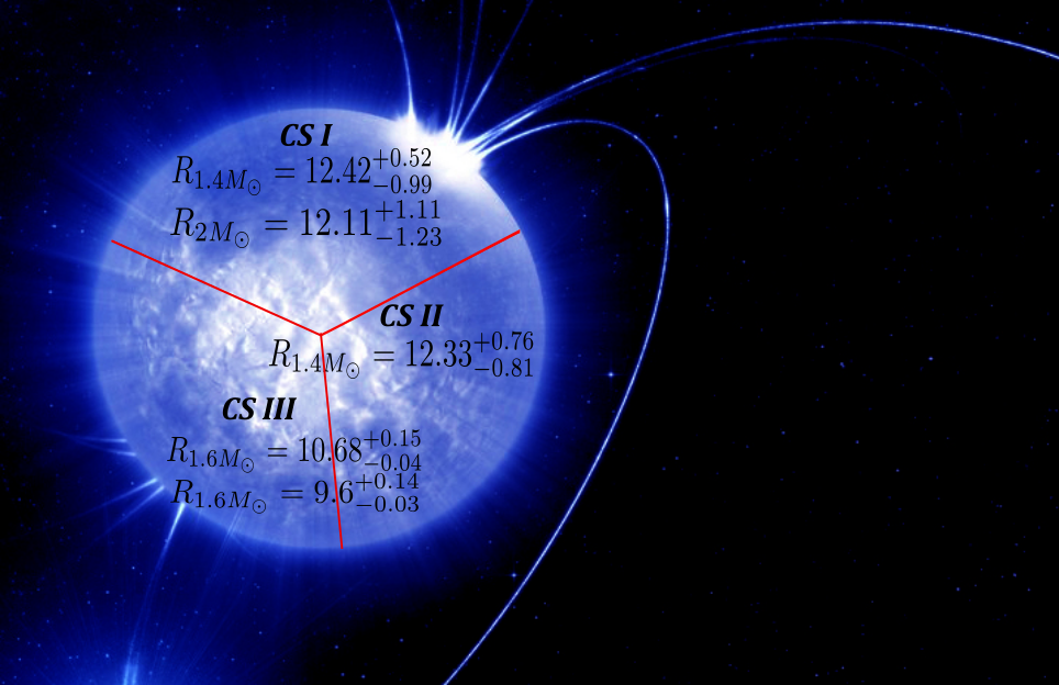
Figure 1: The constraints CSI Altiparmak:2022bke , CSII Raaijmakers:2021uju and CSIII Bauswein:2017vtn . This figure is inspired from Credit: ESO/L.Calçada: https://www.eso.org/public/images/eso0831a/.

For the numerical analysis, in the case of induced inflation we shall use the values $\xi\sim\mathcal{O}(10^{5})$, $\lambda\sim\mathcal{O}(1)$ and for the quadratic inflationary attractor we shall use $\xi\sim\mathcal{O}(10^{-2})$, $\lambda\sim\mathcal{O}(1)$ and $g_{1}\sim\mathcal{O}(10^{-4})$, in order to have a viable phenomenology. Contrary to what is usually done in similar astrophysical works in the literature, the free parameters of specific non-minimally coupled theories in the Einstein frame, including the $R^{2}$ model, are not free parameters of the theory. As we showed earlier these parameters are constrained by the inflationary theory, so these must take specific values.

Table 1: CSI vs the Induced and Quadratic Attractors for the SLy, APR and WFF1 Equations of State for neutron stars Masses $M\sim 2M_{\odot}$

Model	APR	SLy	WFF1
Quadratic Attractors Masses	$M_{APR}=0.709\,M_{\odot}$	$M_{SLy}=2.119\,M_{\odot}$	$M_{WFF1}=0.290\,M_{\odot}$
Quadratic Attractors Radii	$R_{APR}=11.414$km	$R_{SLy}=10.898$km	$R_{WFF1}=11.468$km
Induced Inflation Attractors Masses	$M_{APR}=2.018\,M_{\odot}$	$M_{SLy}=2.017\,M_{\odot}$	$M_{WFF1}=0.340\,M_{\odot}$
Induced Inflation Attractors Radii	$R_{APR}=11.155$km	$R_{SLy}=11.291$km	$R_{WFF1}=11.069$km

The spacetime metric which describes static neutron stars is,

$$ds^{2}=-e^{\nu(r)}dt^{2}+\frac{dr^{2}}{1-\frac{2m(r)}{r}}+r^{2}(d\theta^{2}+\sin^{2}\theta d\phi^{2})\,,$$ (28)

with the function $m(r)$ describing the gravitational mass of the neutron stars and $r$ is the circumferential radius. Our aim is to find numerically the functions $\nu(r)$ and $\frac{1}{1-\frac{2m(r)}{r}}$. The procedure is the following, the function $\nu(r)$ is assumed to have a non-zero central value at the center of the star.

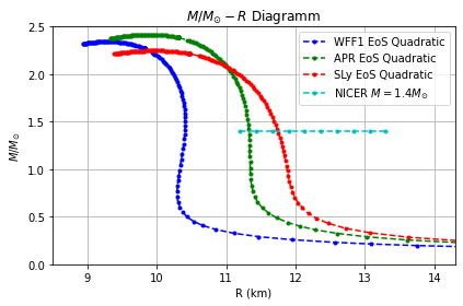
Figure 2: The $M-R$ graphs for the quadratic attractor model for the WFF1, APR and SLy equations of state.

Beyond the surface of the star, in contrast to the General Relativity case, there is no matching with the Schwarzschild metric, because the metric functions receive contribution from the scalar field effects, thus the only matching of the metric above with the Schwarzschild metric will be done at numerical infinity. Indeed, the presence of the scalar potential, and of the function $A(\varphi)$ crucially affects the metric functions beyond the surface of the star, thus no matching at the surface of the star is required. The whole scalarization procedure is based on the effects of the scalar field beyond the surface of the star.

Table 2: CSI vs the Induced and Quadratic Attractors for the SLy, APR and WFF1 Equations of State for neutron stars Masses $M\sim 1.4M_{\odot}$

Model	APR	SLy	WFF1
Quadratic Attractors Masses	$M_{APR}=0.650\,M_{\odot}$	$M_{SLy}=1.425\,M_{\odot}$	$M_{WFF1}=0.258\,M_{\odot}$
Quadratic Attractors Radii	$R_{APR}=11.455$km	$R_{SLy}=11.733$km	$R_{WFF1}=11.951$km
Induced Inflation Attractors Masses	$M_{APR}=0.620\,M_{\odot}$	$M_{SLy}=1.392\,M_{\odot}$	$M_{WFF1}=0.270\,M_{\odot}$
Induced Inflation Attractors Radii	$R_{APR}=11.487$km	$R_{SLy}=11.777$km	$R_{WFF1}=11.892$km

The Tolman-Oppenheimer-Volkoff equations for the scalar-tensor theory in the Einstein frame are,

$$\frac{dm}{dr}=4\pi r^{2}A^{4}(\varphi)\varepsilon+\frac{r}{2}(r-2m(r))\omega^{2}+4\pi r^{2}V(\varphi)\,,$$ (29)

$$\frac{d\nu}{dr}=r\omega^{2}+\frac{2}{r(r-2m(r))}\Big{[}4\pi A^{4}(\varphi)r^{3}P-4\pi V(\varphi)r^{3}\Big{]}+\frac{2m(r)}{r(r-2m(r))}\,,$$ (30)

$$\frac{d\omega}{dr}=\frac{4\pi rA^{4}(\varphi)}{r-2m(r)}\Big{(}\alpha(\varphi)(\epsilon-3P)+r\omega(\epsilon-P)\Big{)}-\frac{2\omega(r-m(r))}{r(r-2m(r))}+\frac{8\pi\omega r^{2}V(\varphi)+r\frac{dV(\varphi)}{d\varphi}}{r-2m(r)}\,,$$ (31)

$$\frac{dP}{dr}=-(\epsilon+P)\Big{[}\frac{1}{2}\frac{d\nu}{dr}+\alpha(\varphi)\omega\Big{]}\,,$$ (32)

$$\omega=\frac{d\varphi}{dr}\,,$$ (33)

and recall that the function $\alpha(\varphi)$ is firstly defined in Eq. (22). With regard to the pressure $P$ and the energy density $\epsilon$, we need to note that these are Jordan frame quantities. Another notable feature is that the spacetime in the interior and the exterior of the neutron star is uniformly described by the spherically symmetric metric (28). However, the Tolman-Oppenheimer-Volkoff equations shall be solved for the interior and the exterior of the star, since beyond the surface, the pressure and energy density are zero. The set of the initial conditions we shall use is the following,

$$P(0)=P_{c}\,,\,\,\,m(0)=0\,,\,\,\,\nu(0)\,,=-\nu_{c}\,,\,\,\,\varphi(0)=\varphi_{c}\,,\,\,\,\omega(0)=0\,.$$ (34)

We shall use a double shooting method in order to determine the values of the metric function $\nu_{c}$ and $\varphi_{c}$ at the center of the star, by optimizing the parameter values using as a rule the optimal decay of the scalar field at the numerical infinity. We shall use three distinct piecewise polytropic equations of state Read:2008iy ; Read:2009yp with the low density part corresponding to the SLy, WFF1 or the APR equations of state. Since the temperature of neutron stars is much lower than the Fermi energy of the particles that constitute neutron stars, the neutron star matter can be described by a one-parameter equation of state that accurately governs cold matter beyond the nuclear density. The problem that arises though is that the uncertainty in the equation of state is large, with the pressure as function of the baryon mass density being uncertain to at least one order of magnitude beyond the nuclear density. Furthermore, the actual phase of matter in the core of neutron stars is also uncertain. Thus a parameterized high-density equation of state can be helpful and an optimal choice of an equation of state is a high-density parameterized equation of state. This piecewise polytropic equation of state, take into account astrophysical phenomenological constraints regarding the nature of neutron stars matter. The piecewise polytropic equation of state we shall use in this paper are also take into account the causality constraints, so causality is respected, see Refs. [111,112] for further details. In general a piecewise polytropic equation of state can be constructed by using a low-density part $\rho<\rho_{0}$, which is usually chosen to be a well-known and tabulated crust equation of state, and also the piecewise polytropic equation of state has a high density part $\rho\gg\rho_{0}$. The numerical analysis we shall perform shall yield the Einstein frame mass of the neutron star, and from this we shall calculate the ADM mass in the Jordan frame, using the following formula Odintsov:2021qbq ; Odintsov:2021nqa ; Oikonomou:2021iid ,

$$M_{J}=A(\varphi(r_{E}))\left(M_{E}-\frac{r_{E}^{2}}{2}\alpha(\varphi(r_{E}))\frac{d\varphi}{dr}\left(2+\alpha(\varphi(r_{E}))r_{E}\frac{d\varphi}{dr}\right)\left(1-\frac{2M_{E}}{r_{E}}\right)\right)\,.$$ (35)

with $r_{E}$ being the radius of the neutron star in the Einstein frame asymptotically and in addition $\frac{d\varphi}{dr}=\frac{d\varphi}{dr}\Big{|}_{r=r_{E}}$. Also, the Jordan and Einstein circumferential radii of the neutron star are related as follows,

$$R=A(\varphi(R_{s}))\,R_{s}\,.$$ (36)

For notational simplicity, we shall denote with $M$ the Jordan frame mass of the star, measured in solar masses $M_{\odot}$ and R denotes the Jordan frame radius expressed in kilometers.

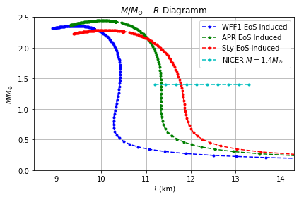
Figure 3: The $M-R$ graphs for the induced inflation attractor model for the WFF1, APR and SLy equations of state.

II.1 Results of the Numerical Analysis

In this subsection we present the results of our numerical analysis. Our aim is to find the $M-R$ graphs for the two inflationary attractor models (Jordan frame quantities) and to confront the data of the $M-R$ graphs with existing constraints on neutron stars masses and radii which were developed nearly after the GW170817 event. We will consider five in total constraints which we classify in three distinct constraints, to which we will refer to as CSI, CSII and CSIII. The CSI was developed in Ref. Altiparmak:2022bke and constrains the radius of an $1.4M_{\odot}$ mass neutron star as $R_{1.4M_{\odot}}=12.42^{+0.52}_{-0.99}$ and the radius of an $2M_{\odot}$ mass neutron star as $R_{2M_{\odot}}=12.11^{+1.11}_{-1.23}\,$km. The constraint CSII was developed in Ref. Raaijmakers:2021uju and constrains the radius of an $1.4M_{\odot}$ mass neutron star to be $R_{1.4M_{\odot}}=12.33^{+0.76}_{-0.81}\,\mathrm{km}$. Finally the constraint CSIII is developed in Ref. Bauswein:2017vtn and constrains the radius of an $1.6M_{\odot}$ mass neutron star to be larger than $R_{1.6M_{\odot}}=12.42^{+0.52}_{-0.99}\,$km while the radius of a neutron star corresponding to the maximum mass must be larger than $R_{M_{max}}>10.68^{+0.15}_{-0.04}\,$km. For reading convenience in Fig. 1 we present the pictorial representation of the constraints CSI, CSII and CSIII on neutron stars.

Table 3: CSII vs the Induced and Quadratic Attractors for the SLy, APR and WFF1 Equations of State for Neutron Star Masses $M\sim 1.4M_{\odot}$

Model	APR	SLy	WFF1
Quadratic Attractors Masses	$M_{APR}=0.593\,M_{\odot}$	$M_{SLy}=1.425\,M_{\odot}$	$M_{WFF1}=0.258\,M_{\odot}$
Quadratic Attractors Radii	$R_{APR}=11.523$km	$R_{SLy}=11.733$km	$R_{WFF1}=11.951$km
Induced Inflation Attractors Masses	$M_{APR}=0.563\,M_{\odot}$	$M_{SLy}=1.392\,M_{\odot}$	$M_{WFF1}=0.270\,M_{\odot}$
Induced Inflation Attractors Radii	$R_{APR}=11.569$km	$R_{SLy}=11.777$km	$R_{WFF1}=11.892$km

For the numerical analysis we shall employ a python 3 numerical code (variant of pyTOV-STT code niksterg ), using the LSODA integrator and a double shooting method for determining the optimal values of the metric function $\nu_{c}$ and of the scalar field $\varphi_{c}$ at the center of the star, which make the scalar field and metric function values vanish at numerical infinity. The numerical infinity is taken to be $r\sim 67.943$ km.

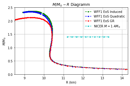
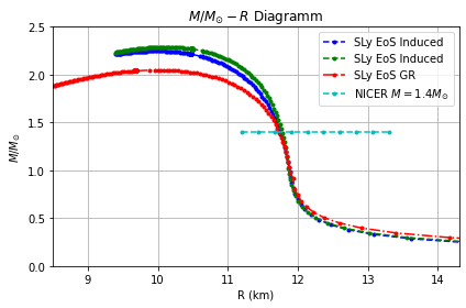
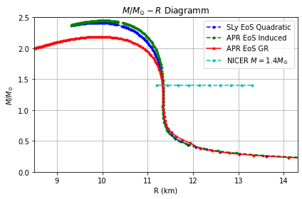
Figure 4: The $M-R$ graphs for the quadratic, induced inflationary attractor models and for the General Relativity case, for the WFF1, APR and SLy equations of state.

For all the plots that follow we added the NICER constraint for $M=1.4M_{\odot}$ neutron stars which $90\%$ credible Miller:2021qha and constrains the neutron stars radius to be $R=11.2-13.3\,$km. To start with, in Figs. 2 and 3 we present the $M-R$ graphs of the quadratic and induced inflationary attractors neutron stars respectively, for the WFF1 equation of state (blue curve), the APR equation of state (green curve) and the SLy equation of state (red curve). As it is apparent, the three distinct equations of state lead to different maximum masses and radii, as it was expected. Also the largest maximum mass is achieved for the stiffer APR equation of state. Also a comparison of the models with the General Relativistic result is given in the three plots of Fig. 4 where we present for each equation of state the $M-R$ graphs of the quadratic attractors (blue curves), the induced attractors (green curves) and the General Relativistic (red curves) for the WFF1 equation of state (upper left plot) the SLy equation of state (upper right) and the APR equation of state (bottom plot). In all cases the maximum masses are larger that those of General Relativity, but the interesting part begins when the constraints CSI, CSII and CSIII are considered.

Table 4: CSIII vs the Induced and Quadratic Attractors for the SLy, APR and WFF1 Equation of State for Neutron Star Masses $M\sim 1.6M_{\odot}$

Model	APR	SLy	WFF1
Quadratic Attractors Masses	$M_{APR}=1.619\,M_{\odot}$	$M_{SLy}=1.584\,M_{\odot}$	$M_{WFF1}=1.606\,M_{\odot}$
Quadratic Attractors Radii	$R_{APR}=11.285$km	$R_{SLy}=11.645$km	$R_{WFF1}=11.115$km
Induced Inflation Attractors Masses	$M_{APR}=1.584\,M_{\odot}$	$M_{SLy}=1.609\,M_{\odot}$	$M_{WFF1}=1.075\,M_{\odot}$
Induced Inflation Attractors Radii	$R_{APR}=11.320$km	$R_{SLy}=11.680$km	$R_{WFF1}=10.423$km

The results of the confrontation of the inflationary attractors models with the observational constraints are presented in Tables 1-5. In Tables 1, 2 we confront the model with the constraint CSI. As it is apparent, the SLy equation of state respects all the constraints for both models, however the WFF1 case violates all the constraints. With regard the APR equation of state, for the induced inflation case respects the second CSI constraint (see Table 2) and also satisfies the CSIII constraint (see Table 3) but violates the rest of the constraints. For the quadratic inflation case, the APR equation of state satisfies only CSIII and violates all the rest. For the WFF1 equation of state, the models violate all the constraints. Thus in conclusion, the only equation of state which provides a viable neutron star phenomenology that respects all the imposed constraints for the induced and quadratic inflationary attractor models is the SLy equation of state. It is apparent that in the post-GW170817 era, a viable phenomenological neutron star model has to pass quite stringent tests in order to be considered viable. Our result indicates that for the models studied, intermediate stiffness equations of state can provide a viable phenomenology, but this is a model dependent result. As we demonstrated, for the quadratic and induced inflation attractors, the only viable result is obtained for the SLy equation of state. This is in contrast with previous work on attractors, which more equation of state could provide a viable phenomenology. The result depends strongly on the shape of the $M-R$ graphs. It seems that the viability is guaranteed for curves strongly bend to the right for radii between 11 km-13 km. In a future work we shall provide a large sample of attractor models and we shall verify this argument in an explicit way.

Table 5: CSIII vs the Induced and Quadratic Attractors for the SLy, APR and WFF1 Equations of State for Maximum Neutron Star Masses

Model	APR	SLy	WFF1
Quadratic Attractors Maximum Masses	$M_{APR}=2.417\,M_{\odot}$	$M_{SLy}=2.248\,M_{\odot}$	$M_{WFF1}=2.342\,M_{\odot}$
Quadratic Attractors Radii	$R_{APR}=9.899$km	$R_{SLy}=9.967$km	$R_{WFF1}=9.281$km
Induced Inflation Attractors Maximum Masses	$M_{APR}=2.018\,M_{\odot}$	$M_{SLy}=2.286\,M_{\odot}$	$M_{WFF1}=2.360\,M_{\odot}$
Induced Inflation Attractors Radii	$R_{APR}=11.155$km	$R_{SLy}=9.981$km	$R_{WFF1}=9.428$km

Before closing this section we need to discuss the necessity of finding the predictions of inflationary potentials on the tidal deformability of neutron stars and also study the radial perturbation effects and the stability of neutron stars in general, by also taking into account the constraints of the GW170817 event. This is a non-trivial task and could be the subject of a distinct article for the various distinct inflationary attractors. For some recent relevant work on the stability properties and perturbations of neutron stars in scalar-tensor and unimodular gravity, see Refs. Brown:2022kbw and Yang:2022ees respectively.

Concluding Remarks

In this work we investigated the neutron star phenomenology of two inflationary attractor potentials, that of quadratic and induced inflation attractor potentials. The two models are known of providing distinct inflationary phenomenology, with the quadratic attractors providing a non-viable inflationary phenomenology, while the induced inflationary attractors provide a viable inflationary phenomenology, identical to the $R^{2}$ model of inflation in the Einstein frame. We extracted the Tolman-Oppenheimer-Volkoff equations in the Einstein frame for both models, and by using a Python 3 LSODA double shooting method we evaluated the masses and radii of neutron stars. From the results we obtained the Jordan frame masses and radii of the neutron stars and we constructed the $M-R$ graphs for three distinct equations of state, the WFF1, the SLy and the APR equation of state. Accordingly, we confronted the models with three constraints that constrain the radii of specific mass neutron stars. Specifically, we considered the three following constraints, the CSI, CSII and CSIII. The CSI is studied in Ref. Altiparmak:2022bke and constrains the radius of an $1.4M_{\odot}$ mass neutron stars to be $R_{1.4M_{\odot}}=12.42^{+0.52}_{-0.99}$ and the radius of an $2M_{\odot}$ mass neutron star to be $R_{2M_{\odot}}=12.11^{+1.11}_{-1.23}\,$km. The constraint CSII was studied in Ref. Raaijmakers:2021uju and constrains the radius of an $1.4M_{\odot}$ mass neutron star to be $R_{1.4M_{\odot}}=12.33^{+0.76}_{-0.81}\,\mathrm{km}$. Finally the constraint CSIII was studied in Ref. Bauswein:2017vtn and constrains the radius of an $1.6M_{\odot}$ mass neutron star to be larger than $R_{1.6M_{\odot}}=12.42^{+0.52}_{-0.99}\,$km while the radius of a neutron star corresponding to the maximum mass must be larger than $R_{M_{max}}>10.68^{+0.15}_{-0.04}\,$km. As we showed, the SLy equation of state respects all the constraints for both models, however the WFF1 case violates all the constraints. With regard the APR equation of state, for the induced inflation case respects the second CSI constraint and also satisfies the CSIII constraint, but violates the rest of the constraints. For the quadratic inflation case, the APR equation of state satisfies only CSIII and violates all the rest. For the WFF1 equation of state, the models violate all the constraints. Thus only the SLy equation of state respects all the constraints for both the induced and quadratic inflation models. Also let us further note that if the two inflationary models are compared for each equation of state, the resulting neutron star phenomenology is quite similar if not almost identical, see for example Fig. 4. This is contrast with the inflationary phenomenology of the two attractor models, which is quite different, since the induced attractors provide a viable inflationary phenomenology while the quadratic attractors are not viable cosmologically. This behavior is not a general rule though, since the opposite can occur, that is, two models might be identical in their inflationary phenomenology, while producing quite different neutron star phenomenology. Work is in progress toward this research line. In general let us comment that it seems that cosmologically indistinguishable models might be discriminated using their neutron star phenomenology and vice versa. Intriguingly enough, scalar models which are indistinguishable at frequencies of primordial cosmological perturbations modes near the Cosmic Microwave Background ones, can be distinguishable in future gravitational waves experiments that can probe a stochastic tensor background. This is the opposite in spirit to what we demonstrated in this paper, the fact that phenomenologically distinguishable theories, can be distinguished using their neutron star predictions. We shall support this argument in future works. We need to note that the present framework is not advantageous over some other modified gravity, it is one possible description of nature, among other modified gravities in general.

With regard to this last perspective, an important comment is in order. In the present work the choice of the function $f(\phi)$ in Eq. (2) is not specified and the potential is actually independent of it and rather universal. This is the major difference with the $\alpha$-attractors case, studied for example in our previous work Odintsov:2021qbq . Also, we need to note that for the quadratic attractors case, these are entirely different from the $\alpha$-attractors case, for an inflationary phenomenology point of view since the tensor-to-scalar ratio and the spectral index in Eq. (15) are different from the ones corresponding to the $\alpha$-attractors. Another useful comment to add is that, although the induced inflation and $\alpha$-attractors have the exact same inflationary phenomenology described by Eq. (12), in spite the fact that these are basically different inflationary theories with the same phenomenology (this justifies the terminology attractors), in neutron stars they lead to different $M-R$ graphs. In a future work we shall directly point out this issue, namely, the fact that although distinct inflationary theories are indistinguishable at the inflationary phenomenology level, they can be actually distinguished in neutron stars.

References

- (1) B. P. Abbott et al. [LIGO Scientific and Virgo], Phys. Rev. Lett. 119 (2017) no.16, 161101 doi:10.1103/PhysRevLett.119.161101 [arXiv:1710.05832 [gr-qc]].
- (2) R. Abbott et al. [LIGO Scientific and Virgo], Astrophys. J. Lett. 896 (2020) no.2, L44 doi:10.3847/2041-8213/ab960f [arXiv:2006.12611 [astro-ph.HE]].
- (3) P. Haensel, A. Y. Potekhin and D. G. Yakovlev, Astrophys. Space Sci. Libr. 326 (2007), pp.1-619 doi:10.1007/978-0-387-47301-7
- (4) J. L. Friedman and N. Stergioulas, “Rotating Relativistic Stars,” doi:10.1017/CBO9780511977596
- (5) G. Baym, T. Hatsuda, T. Kojo, P. D. Powell, Y. Song and T. Takatsuka, Rept. Prog. Phys. 81 (2018) no.5, 056902 doi:10.1088/1361-6633/aaae14 [arXiv:1707.04966 [astro-ph.HE]].
- (6) J. M. Lattimer and M. Prakash, Science 304 (2004), 536-542 doi:10.1126/science.1090720 [arXiv:astro-ph/0405262 [astro-ph]].
- (7) G. J. Olmo, D. Rubiera-Garcia and A. Wojnar, Phys. Rept. 876 (2020), 1-75 doi:10.1016/j.physrep.2020.07.001 [arXiv:1912.05202 [gr-qc]].
- (8) J. M. Lattimer, Ann. Rev. Nucl. Part. Sci. 62 (2012), 485-515 doi:10.1146/annurev-nucl-102711-095018 [arXiv:1305.3510 [nucl-th]].
- (9) A. W. Steiner and S. Gandolfi, Phys. Rev. Lett. 108 (2012), 081102 doi:10.1103/PhysRevLett.108.081102 [arXiv:1110.4142 [nucl-th]].
- (10) C. J. Horowitz, M. A. Perez-Garcia, D. K. Berry and J. Piekarewicz, Phys. Rev. C 72 (2005), 035801 doi:10.1103/PhysRevC.72.035801 [arXiv:nucl-th/0508044 [nucl-th]].
- (11) G. Watanabe, K. Iida and K. Sato, Nucl. Phys. A 676 (2000), 455-473 [erratum: Nucl. Phys. A 726 (2003), 357-365] doi:10.1016/S0375-9474(00)00197-4 [arXiv:astro-ph/0001273 [astro-ph]].
- (12) H. Shen, H. Toki, K. Oyamatsu and K. Sumiyoshi, Nucl. Phys. A 637 (1998), 435-450 doi:10.1016/S0375-9474(98)00236-X [arXiv:nucl-th/9805035 [nucl-th]].
- (13) J. Xu, L. W. Chen, B. A. Li and H. R. Ma, Astrophys. J. 697 (2009), 1549-1568 doi:10.1088/0004-637X/697/2/1549 [arXiv:0901.2309 [astro-ph.SR]].
- (14) K. Hebeler, J. M. Lattimer, C. J. Pethick and A. Schwenk, Astrophys. J. 773 (2013), 11 doi:10.1088/0004-637X/773/1/11 [arXiv:1303.4662 [astro-ph.SR]].
- (15) J. de Jesús Mendoza-Temis, M. R. Wu, G. Martínez-Pinedo, K. Langanke, A. Bauswein and H. T. Janka, Phys. Rev. C 92 (2015) no.5, 055805 doi:10.1103/PhysRevC.92.055805 [arXiv:1409.6135 [astro-ph.HE]].
- (16) W. C. G. Ho, K. G. Elshamouty, C. O. Heinke and A. Y. Potekhin, Phys. Rev. C 91 (2015) no.1, 015806 doi:10.1103/PhysRevC.91.015806 [arXiv:1412.7759 [astro-ph.HE]].
- (17) A. Kanakis-Pegios, P. S. Koliogiannis and C. C. Moustakidis, [arXiv:2012.09580 [astro-ph.HE]].
- (18) L. Tsaloukidis, P. S. Koliogiannis, A. Kanakis-Pegios and C. C. Moustakidis, [arXiv:2210.15644 [astro-ph.HE]].
- (19) M. Buschmann, R. T. Co, C. Dessert and B. R. Safdi, Phys. Rev. Lett. 126 (2021) no.2, 021102 doi:10.1103/PhysRevLett.126.021102 [arXiv:1910.04164 [hep-ph]].
- (20) B. R. Safdi, Z. Sun and A. Y. Chen, Phys. Rev. D 99 (2019) no.12, 123021 doi:10.1103/PhysRevD.99.123021 [arXiv:1811.01020 [astro-ph.CO]].
- (21) A. Hook, Y. Kahn, B. R. Safdi and Z. Sun, Phys. Rev. Lett. 121 (2018) no.24, 241102 doi:10.1103/PhysRevLett.121.241102 [arXiv:1804.03145 [hep-ph]].
- (22) T. D. P. Edwards, B. J. Kavanagh, L. Visinelli and C. Weniger, [arXiv:2011.05378 [hep-ph]].
- (23) S. Nurmi, E. D. Schiappacasse and T. T. Yanagida, [arXiv:2102.05680 [hep-ph]].
- (24) A. V. Astashenok, S. Capozziello, S. D. Odintsov and V. K. Oikonomou, Phys. Lett. B 811 (2020), 135910 doi:10.1016/j.physletb.2020.135910 [arXiv:2008.10884 [gr-qc]].
- (25) A. V. Astashenok, S. Capozziello, S. D. Odintsov and V. K. Oikonomou, [arXiv:2103.04144 [gr-qc]].
- (26) S. Capozziello, M. De Laurentis, R. Farinelli and S. D. Odintsov, Phys. Rev. D 93 (2016) no.2, 023501 doi:10.1103/PhysRevD.93.023501 [arXiv:1509.04163 [gr-qc]].
- (27) A. V. Astashenok, S. Capozziello and S. D. Odintsov, JCAP 01 (2015), 001 doi:10.1088/1475-7516/2015/01/001 [arXiv:1408.3856 [gr-qc]].
- (28) A. V. Astashenok, S. Capozziello and S. D. Odintsov, Phys. Rev. D 89 (2014) no.10, 103509 doi:10.1103/PhysRevD.89.103509 [arXiv:1401.4546 [gr-qc]].
- (29) A. V. Astashenok, S. Capozziello and S. D. Odintsov, JCAP 12 (2013), 040 doi:10.1088/1475-7516/2013/12/040 [arXiv:1309.1978 [gr-qc]].
- (30) A. S. Arapoglu, C. Deliduman and K. Y. Eksi, JCAP 07 (2011), 020 doi:10.1088/1475-7516/2011/07/020 [arXiv:1003.3179 [gr-qc]].
- (31) G. Panotopoulos, T. Tangphati, A. Banerjee and M. K. Jasim, [arXiv:2104.00590 [gr-qc]].
- (32) R. Lobato, O. Lourenço, P. H. R. S. Moraes, C. H. Lenzi, M. de Avellar, W. de Paula, M. Dutra and M. Malheiro, JCAP 12 (2020), 039 doi:10.1088/1475-7516/2020/12/039 [arXiv:2009.04696 [astro-ph.HE]].
- (33) K. Numajiri, T. Katsuragawa and S. Nojiri, Phys. Lett. B 826 (2022), 136929 doi:10.1016/j.physletb.2022.136929 [arXiv:2111.02660 [gr-qc]].
- (34) S. Altiparmak, C. Ecker and L. Rezzolla, [arXiv:2203.14974 [astro-ph.HE]].
- (35) A. Bauswein, G. Guo, J. H. Lien, Y. H. Lin and M. R. Wu, [arXiv:2012.11908 [astro-ph.HE]].
- (36) S. Vretinaris, N. Stergioulas and A. Bauswein, Phys. Rev. D 101 (2020) no.8, 084039 doi:10.1103/PhysRevD.101.084039 [arXiv:1910.10856 [gr-qc]].
- (37) A. Bauswein, S. Blacker, V. Vijayan, N. Stergioulas, K. Chatziioannou, J. A. Clark, N. U. F. Bastian, D. B. Blaschke, M. Cierniak and T. Fischer, Phys. Rev. Lett. 125 (2020) no.14, 141103 doi:10.1103/PhysRevLett.125.141103 [arXiv:2004.00846 [astro-ph.HE]].
- (38) A. Bauswein, O. Just, H. T. Janka and N. Stergioulas, Astrophys. J. Lett. 850 (2017) no.2, L34 doi:10.3847/2041-8213/aa9994 [arXiv:1710.06843 [astro-ph.HE]].
- (39) E. R. Most, L. R. Weih, L. Rezzolla and J. Schaffner-Bielich, Phys. Rev. Lett. 120 (2018) no.26, 261103 doi:10.1103/PhysRevLett.120.261103 [arXiv:1803.00549 [gr-qc]].
- (40) L. Rezzolla, E. R. Most and L. R. Weih, Astrophys. J. Lett. 852 (2018) no.2, L25 doi:10.3847/2041-8213/aaa401 [arXiv:1711.00314 [astro-ph.HE]].
- (41) A. Nathanail, E. R. Most and L. Rezzolla, Astrophys. J. Lett. 908 (2021) no.2, L28 doi:10.3847/2041-8213/abdfc6 [arXiv:2101.01735 [astro-ph.HE]].
- (42) S. Köppel, L. Bovard and L. Rezzolla, Astrophys. J. Lett. 872 (2019) no.1, L16 doi:10.3847/2041-8213/ab0210 [arXiv:1901.09977 [gr-qc]].
- (43) G. Raaijmakers, S. K. Greif, K. Hebeler, T. Hinderer, S. Nissanke, A. Schwenk, T. E. Riley, A. L. Watts, J. M. Lattimer and W. C. G. Ho, Astrophys. J. Lett. 918 (2021) no.2, L29 doi:10.3847/2041-8213/ac089a [arXiv:2105.06981 [astro-ph.HE]].
- (44) E. R. Most, L. J. Papenfort, S. Tootle and L. Rezzolla, Astrophys. J. 912 (2021) no.1, 80 doi:10.3847/1538-4357/abf0a5 [arXiv:2012.03896 [astro-ph.HE]].
- (45) C. Ecker and L. Rezzolla, [arXiv:2209.08101 [astro-ph.HE]].
- (46) J. L. Jiang, C. Ecker and L. Rezzolla, [arXiv:2211.00018 [gr-qc]].
- (47) P. Pani and E. Berti, Phys. Rev. D 90 (2014) no.2, 024025 doi:10.1103/PhysRevD.90.024025 [arXiv:1405.4547 [gr-qc]].
- (48) K. V. Staykov, D. D. Doneva, S. S. Yazadjiev and K. D. Kokkotas, JCAP 10 (2014), 006 doi:10.1088/1475-7516/2014/10/006 [arXiv:1407.2180 [gr-qc]].
- (49) M. Horbatsch, H. O. Silva, D. Gerosa, P. Pani, E. Berti, L. Gualtieri and U. Sperhake, Class. Quant. Grav. 32 (2015) no.20, 204001 doi:10.1088/0264-9381/32/20/204001 [arXiv:1505.07462 [gr-qc]].
- (50) H. O. Silva, C. F. B. Macedo, E. Berti and L. C. B. Crispino, Class. Quant. Grav. 32 (2015), 145008 doi:10.1088/0264-9381/32/14/145008 [arXiv:1411.6286 [gr-qc]].
- (51) D. D. Doneva, S. S. Yazadjiev, N. Stergioulas and K. D. Kokkotas, Phys. Rev. D 88 (2013) no.8, 084060 doi:10.1103/PhysRevD.88.084060 [arXiv:1309.0605 [gr-qc]].
- (52) R. Xu, Y. Gao and L. Shao, Phys. Rev. D 102 (2020) no.6, 064057 doi:10.1103/PhysRevD.102.064057 [arXiv:2007.10080 [gr-qc]].
- (53) M. Salgado, D. Sudarsky and U. Nucamendi, Phys. Rev. D 58 (1998), 124003 doi:10.1103/PhysRevD.58.124003 [arXiv:gr-qc/9806070 [gr-qc]].
- (54) M. Shibata, K. Taniguchi, H. Okawa and A. Buonanno, Phys. Rev. D 89 (2014) no.8, 084005 doi:10.1103/PhysRevD.89.084005 [arXiv:1310.0627 [gr-qc]].
- (55) A. Savaş Arapoğlu, K. Yavuz Ekşi and A. Emrah Yükselci, Phys. Rev. D 99 (2019) no.6, 064055 doi:10.1103/PhysRevD.99.064055 [arXiv:1903.00391 [gr-qc]].
- (56) F. M. Ramazanoğlu and F. Pretorius, Phys. Rev. D 93 (2016) no.6, 064005 doi:10.1103/PhysRevD.93.064005 [arXiv:1601.07475 [gr-qc]].
- (57) Z. Altaha Motahar, J. L. Blázquez-Salcedo, D. D. Doneva, J. Kunz and S. S. Yazadjiev, Phys. Rev. D 99 (2019) no.10, 104006 doi:10.1103/PhysRevD.99.104006 [arXiv:1902.01277 [gr-qc]].
- (58) X. Y. Chew, V. Dzhunushaliev, V. Folomeev, B. Kleihaus and J. Kunz, Phys. Rev. D 100 (2019) no.4, 044019 doi:10.1103/PhysRevD.100.044019 [arXiv:1906.08742 [gr-qc]].
- (59) J. L. Blázquez-Salcedo, F. Scen Khoo and J. Kunz, EPL 130 (2020) no.5, 50002 doi:10.1209/0295-5075/130/50002 [arXiv:2001.09117 [gr-qc]].
- (60) Z. Altaha Motahar, J. L. Blázquez-Salcedo, B. Kleihaus and J. Kunz, Phys. Rev. D 96 (2017) no.6, 064046 doi:10.1103/PhysRevD.96.064046 [arXiv:1707.05280 [gr-qc]].
- (61) S. D. Odintsov and V. K. Oikonomou, Phys. Dark Univ. 32 (2021), 100805 doi:10.1016/j.dark.2021.100805 [arXiv:2103.07725 [gr-qc]].
- (62) S. D. Odintsov and V. K. Oikonomou, Annals Phys. 440 (2022), 168839 doi:10.1016/j.aop.2022.168839 [arXiv:2104.01982 [gr-qc]].
- (63) V. K. Oikonomou, Class. Quant. Grav. 38 (2021) no.17, 175005 doi:10.1088/1361-6382/ac161c [arXiv:2107.12430 [gr-qc]].
- (64) J. M. Z. Pretel, J. D. V. Arbañil, S. B. Duarte, S. E. Jorás and R. R. R. Reis, [arXiv:2206.03878 [gr-qc]].
- (65) J. M. Z. Pretel and S. B. Duarte, [arXiv:2202.04467 [gr-qc]].
- (66) R. R. Cuzinatto, C. A. M. de Melo, L. G. Medeiros and P. J. Pompeia, Phys. Rev. D 93 (2016) no.12, 124034 [erratum: Phys. Rev. D 98 (2018) no.2, 029901] doi:10.1103/PhysRevD.93.124034 [arXiv:1603.01563 [gr-qc]].
- (67) R. Kallosh, A. Linde and D. Roest, JHEP 09 (2014), 062 doi:10.1007/JHEP09(2014)062 [arXiv:1407.4471 [hep-th]].
- (68) R. Kallosh and A. Linde, JCAP 1307 (2013) 002 [arXiv:1306.5220 [hep-th]].
- (69) S. Ferrara, R. Kallosh, A. Linde and M. Porrati, Phys. Rev. D 88 (2013) no.8, 085038 [arXiv:1307.7696 [hep-th]].
- (70) R. Kallosh, A. Linde and D. Roest, JHEP 1311 (2013) 198 [arXiv:1311.0472 [hep-th]].
- (71) JCAP 05 (2015), 003 doi:10.1088/1475-7516/2015/05/003 [arXiv:1504.00663 [hep-th]].
- (72) S. Cecotti and R. Kallosh, JHEP 1405 (2014) 114 [arXiv:1403.2932 [hep-th]].
- (73) J. J. M. Carrasco, R. Kallosh and A. Linde, JHEP 1510 (2015) 147 [arXiv:1506.01708 [hep-th]].
- (74) J. J. M. Carrasco, R. Kallosh, A. Linde and D. Roest, Phys. Rev. D 92 (2015) no.4, 041301 doi:10.1103/PhysRevD.92.041301 [arXiv:1504.05557 [hep-th]].
- (75) R. Kallosh, A. Linde and D. Roest, Phys. Rev. Lett. 112 (2014) no.1, 011303 doi:10.1103/PhysRevLett.112.011303 [arXiv:1310.3950 [hep-th]].
- (76) D. Roest and M. Scalisi, Phys. Rev. D 92 (2015) 043525 doi:10.1103/PhysRevD.92.043525 [arXiv:1503.07909 [hep-th]].
- (77) R. Kallosh, A. Linde and D. Roest, JHEP 1408 (2014) 052 doi:10.1007/JHEP08(2014)052 [arXiv:1405.3646 [hep-th]].
- (78) J. Ellis, D. V. Nanopoulos and K. A. Olive, JCAP 1310 (2013) 009 [arXiv:1307.3537 [hep-th]].
- (79) Y. F. Cai, J. O. Gong and S. Pi, Phys. Lett. B 738 (2014) 20 doi:10.1016/j.physletb.2014.09.009 [arXiv:1404.2560 [hep-th]].
- (80) Z. Yi and Y. Gong, arXiv:1608.05922 [gr-qc].
- (81) Y. Akrami, R. Kallosh, A. Linde and V. Vardanyan, JCAP 06 (2018), 041 doi:10.1088/1475-7516/2018/06/041 [arXiv:1712.09693 [hep-th]].
- (82) S. Qummer, A. Jawad and M. Younas, Int. J. Mod. Phys. D 29 (2020) no.16, 2050117 doi:10.1142/S0218271820501175
- (83) Q. Fei, Z. Yi and Y. Yang, Universe 6 (2020) no.11, 213 doi:10.3390/universe6110213 [arXiv:2009.14819 [gr-qc]].
- (84) A. D. Kanfon, F. Mavoa and S. M. J. Houndjo, Astrophys. Space Sci. 365 (2020) no.6, 97 doi:10.1007/s10509-020-03813-6
- (85) I. Antoniadis, A. Karam, A. Lykkas, T. Pappas and K. Tamvakis, PoS CORFU2019 (2020), 073 doi:10.22323/1.376.0073 [arXiv:1912.12757 [gr-qc]].
- (86) C. García-García, P. Ruíz-Lapuente, D. Alonso and M. Zumalacárregui, JCAP 07 (2019), 025 doi:10.1088/1475-7516/2019/07/025 [arXiv:1905.03753 [astro-ph.CO]].
- (87) F. X. Linares Cedeño, A. Montiel, J. C. Hidalgo and G. Germán, JCAP 08 (2019), 002 doi:10.1088/1475-7516/2019/08/002 [arXiv:1905.00834 [gr-qc]].
- (88) S. Karamitsos, JCAP 09 (2019), 022 doi:10.1088/1475-7516/2019/09/022 [arXiv:1903.03707 [hep-th]].
- (89) D. D. Canko, I. D. Gialamas and G. P. Kodaxis, Eur. Phys. J. C 80 (2020) no.5, 458 doi:10.1140/epjc/s10052-020-8025-4 [arXiv:1901.06296 [hep-th]].
- (90) T. Miranda, C. Escamilla-Rivera, O. F. Piattella and J. C. Fabris, JCAP 05 (2019), 028 doi:10.1088/1475-7516/2019/05/028 [arXiv:1812.01287 [gr-qc]].
- (91) A. Karam, T. Pappas and K. Tamvakis, JCAP 02 (2019), 006 doi:10.1088/1475-7516/2019/02/006 [arXiv:1810.12884 [gr-qc]].
- (92) K. Nozari and N. Rashidi, Astrophys. J. 863 (2018) no.2, 133 doi:10.3847/1538-4357/aad18e [arXiv:1808.05363 [astro-ph.CO]].
- (93) C. García-García, E. V. Linder, P. Ruíz-Lapuente and M. Zumalacárregui, JCAP 08 (2018), 022 doi:10.1088/1475-7516/2018/08/022 [arXiv:1803.00661 [astro-ph.CO]].
- (94) N. Rashidi and K. Nozari, Int. J. Mod. Phys. D 27 (2018) no.07, 1850076 doi:10.1142/S0218271818500761 [arXiv:1802.09185 [astro-ph.CO]].
- (95) Q. Gao, Y. Gong and Q. Fei, JCAP 05 (2018), 005 doi:10.1088/1475-7516/2018/05/005 [arXiv:1801.09208 [gr-qc]].
- (96) K. Dimopoulos, L. Donaldson Wood and C. Owen, Phys. Rev. D 97 (2018) no.6, 063525 doi:10.1103/PhysRevD.97.063525 [arXiv:1712.01760 [astro-ph.CO]].
- (97) T. Miranda, J. C. Fabris and O. F. Piattella, JCAP 09 (2017), 041 doi:10.1088/1475-7516/2017/09/041 [arXiv:1707.06457 [gr-qc]].
- (98) A. Karam, T. Pappas and K. Tamvakis, Phys. Rev. D 96 (2017) no.6, 064036 doi:10.1103/PhysRevD.96.064036 [arXiv:1707.00984 [gr-qc]].
- (99) K. Nozari and N. Rashidi, Phys. Rev. D 95 (2017) no.12, 123518 doi:10.1103/PhysRevD.95.123518 [arXiv:1705.02617 [astro-ph.CO]].
- (100) Q. Gao and Y. Gong, Eur. Phys. J. Plus 133 (2018) no.11, 491 doi:10.1140/epjp/i2018-12324-3 [arXiv:1703.02220 [gr-qc]].
- (101) C. Q. Geng, C. C. Lee and Y. P. Wu, Eur. Phys. J. C 77 (2017) no.3, 162 doi:10.1140/epjc/s10052-017-4720-1 [arXiv:1512.04019 [astro-ph.CO]].
- (102) S. D. Odintsov and V. K. Oikonomou, Phys. Lett. B 807 (2020), 135576 doi:10.1016/j.physletb.2020.135576 [arXiv:2005.12804 [gr-qc]].
- (103) S. D. Odintsov and V. K. Oikonomou, Phys. Rev. D 94 (2016) no.12, 124026 doi:10.1103/PhysRevD.94.124026 [arXiv:1612.01126 [gr-qc]].
- (104) S. D. Odintsov and V. K. Oikonomou, Class. Quant. Grav. 34 (2017) no.10, 105009 doi:10.1088/1361-6382/aa69a8 [arXiv:1611.00738 [gr-qc]].
- (105) L. Järv, A. Karam, A. Kozak, A. Lykkas, A. Racioppi and M. Saal, Phys. Rev. D 102 (2020) no.4, 044029 doi:10.1103/PhysRevD.102.044029 [arXiv:2005.14571 [gr-qc]].
- (106) Y. Akrami et al. [Planck], Astron. Astrophys. 641 (2020), A10 doi:10.1051/0004-6361/201833887 [arXiv:1807.06211 [astro-ph.CO]].
- (107) Nikolaos Stergioulas, https://github.com/niksterg
- (108) J. S. Read, B. D. Lackey, B. J. Owen and J. L. Friedman, Phys. Rev. D 79 (2009), 124032
- (109) J. S. Read, C. Markakis, M. Shibata, K. Uryu, J. D. E. Creighton and J. L. Friedman, Phys. Rev. D 79 (2009), 124033
- (110) R. B. Wiringa, V. Fiks and A. Fabrocini, Phys. Rev. C 38 (1988), 1010-1037 doi:10.1103/PhysRevC.38.1010
- (111) F. Douchin and P. Haensel, Astron. Astrophys. 380 (2001), 151 doi:10.1051/0004-6361:20011402 [arXiv:astro-ph/0111092 [astro-ph]].
- (112) A. Akmal, V. R. Pandharipande and D. G. Ravenhall, Phys. Rev. C 58 (1998), 1804-1828 doi:10.1103/PhysRevC.58.1804 [arXiv:nucl-th/9804027 [nucl-th]].
- (113) R. Arnowitt, S. Deser and C. W. Misner, Phys. Rev. 118 (1960), 1100-1104 doi:10.1103/PhysRev.118.1100
- (114) D. I. Kaiser, Phys. Rev. D 52 (1995), 4295-4306 doi:10.1103/PhysRevD.52.4295 [arXiv:astro-ph/9408044 [astro-ph]].
- (115) Valerio Faraoni, Cosmology in Scalar-Tensor Gravity, Springer 2004
-
(116)
P Moniz, P Crawford, A Barroso, Class. Quantum Grav. 7
L143 (1990);
https://doi.org/10.1088/0264-9381/7/7/005 - (117) R. Santos, [arXiv:2207.14057 [hep-ph]].
- (118) M. C. Miller, F. K. Lamb, A. J. Dittmann, S. Bogdanov, Z. Arzoumanian, K. C. Gendreau, S. Guillot, W. C. G. Ho, J. M. Lattimer and M. Loewenstein, et al. Astrophys. J. Lett. 918 (2021) no.2, L28 doi:10.3847/2041-8213/ac089b [arXiv:2105.06979 [astro-ph.HE]].
- (119) S. M. Brown, [arXiv:2210.14025 [gr-qc]].
- (120) R. X. Yang, F. Xie and D. J. Liu, [arXiv:2211.00278 [gr-qc]].