Trust your neighbours:
Penalty-based constraints for model calibration

Abstract

Ensuring reliable confidence scores from deep networks is of pivotal importance in critical decision-making systems, notably in the medical domain. While recent literature on calibrating deep segmentation networks has led to significant progress, their uncertainty is usually modeled by leveraging the information of individual pixels, which disregards the local structure of the object of interest. In particular, only the recent Spatially Varying Label Smoothing (SVLS) approach addresses this issue by softening the pixel label assignments with a discrete spatial Gaussian kernel. In this work, we first present a constrained optimization perspective of SVLS and demonstrate that it enforces an implicit constraint on soft class proportions of surrounding pixels. Furthermore, our analysis shows that SVLS lacks a mechanism to balance the contribution of the constraint with the primary objective, potentially hindering the optimization process. Based on these observations, we propose a principled and simple solution based on equality constraints on the logit values, which enables to control explicitly both the enforced constraint and the weight of the penalty, offering more flexibility. Comprehensive experiments on a variety of well-known segmentation benchmarks demonstrate the superior performance of the proposed approach. The code is available at https://github.com/Bala93/MarginLoss

egmentation, Calibration, Uncertainty estimation

1 Introduction

Deep neural networks (DNNs) have achieved remarkable success in important areas of various domains, such as computer vision, machine learning and natural language processing. Nevertheless, there exists growing evidence that suggests that these models are poorly calibrated, leading to overconfident predictions that may assign high confidence to incorrect predictions [5, 6]. This represents a major problem, as inaccurate uncertainty estimates can have severe consequences in safety-critical applications such as medical diagnosis. The underlying cause of network miscalibration is hypothesized to be the high capacity of these models, which makes them susceptible to overfitting on the negative log-likelihood loss that is conventionally used during training [6].

In light of the significance of this issue, there has been a surge in popularity for quantifying the predictive uncertainty in modern DNNs. A simple approach involves a post-processing step that modifies the softmax probability predictions of an already trained network [4, 6, 23, 24]. Despite its efficiency, this family of approaches presents important limitations, which include i) a dataset-dependency on the value of the transformation parameters and ii) a large degradation observed under distributional drifts [20]. A more principled solution integrates a term that penalizes confident output distributions into the learning objective, which explicitly maximizes the Shannon entropy of the model predictions during training [21]. Furthermore, findings from recent works on calibration [16, 17] have demonstrated that popular classification losses, such as Label Smoothing (LS) [22] and Focal Loss (FL) [10], have a favorable effect on model calibration, as they implicitly integrate an entropy maximization objective. Following these works, [11, 18] presented a unified view of state-of-the-art calibration approaches [21, 22, 10] showing that these strategies can be viewed as approximations of a linear penalty imposing equality constraints on logit distances. The associated equality constraint results in gradients that continually push towards a non-informative solution, potentially hindering the ability to achieve the optimal balance between discriminative performance and model calibration. To alleviate this limitation, [11, 18] proposed a simple and flexible alternative based on inequality constraints, which imposes a controllable margin on logit distances. Despite the progress brought by these methods, none of them explicitly considers pixel relationships, which is fundamental in the context of image segmentation.

Indeed, the nature of structured predictions in segmentation, involves pixel-wise classification based on spatial dependencies, which limits the effectiveness of these strategies to yield performances similar to those observed in classification tasks. In particular, this potentially suboptimal performance can be attributed to the uniform (or near-to-uniform) distribution enforced on the softmax/logits distributions, which disregards the spatial context information. To address this important issue, Spatially Varying Label Smoothing (SVLS) [7] introduces a soft labeling approach that captures the structural uncertainty required in semantic segmentation. In practice, smoothing the hard-label assignment is achieved through a Gaussian kernel applied across the one-hot encoded ground truth, which results in soft class probabilities based on neighboring pixels. Nevertheless, while the reasoning behind this smoothing strategy relies on the intuition of giving an equal contribution to the central label and all surrounding labels combined, its impact on the training, from an optimization standpoint, has not been studied.

The contributions of this work can be summarized as follows:

• We provide a constrained-optimization perspective of Spatially Varying Label Smoothing (SVLS) [7], demonstrating that it imposes an implicit constraint on a soft class proportion of surrounding pixels. Our formulation shows that SVLS lacks a mechanism to control explicitly the importance of the constraint, which may hinder the optimization process as it becomes challenging to balance the constraint with the primary objective effectively.

• Following our observations, we propose a simple and flexible solution based on equality constraints on the logit distributions. The proposed constraint is enforced with a simple linear penalty, which incorporates an explicit mechanism to control the weight of the penalty. Our approach not only offers a more efficient strategy to model the logit distributions but implicitly decreases the logit values, which results in less overconfident predictions.

• Comprehensive experiments over multiple medical image segmentation benchmarks, including diverse targets and modalities, show the superiority of our method compared to state-of-the-art calibration losses.

2 Methodology

Formulation. Let us denote the training dataset as $\mathcal{D}(\mathcal{X},\mathcal{Y})=\{(\mathbf{x}^{(n)},\mathbf{y}^{(n)})\}_{n=1}^{N}$, with $\mathbf{x}^{(n)}\in\mathcal{X}\subset\mathbb{R}^{\Omega_{n}}$ representing the $n^{th}$ image, $\Omega_{n}$ the spatial image domain, and $\mathbf{y}^{(n)}\in\mathcal{Y}\subset\mathbb{R}^{K}$ its corresponding ground-truth label with $K$ classes, provided as a one-hot encoding vector. Given an input image $\mathbf{x}^{(n)}$, a neural network parameterized by $\theta$ generates a softmax probability vector, defined as $f_{\theta}(\mathbf{x}^{(n)})=\mathbf{s}^{(n)}\in\mathbb{R}^{\Omega_{n}\times K}$, where $\mathbf{s}$ is obtained after applying the softmax function over the logits ${\mathbf{l}}^{(n)}\in\mathbb{R}^{\Omega_{n}\times K}$. To simplify the notations, we omit sample indices, as this does not lead to any ambiguity.

2.1 A constrained optimization perspective of SVLS

Spatially Varying Label Smoothing (SVLS) [7] considers the surrounding class distribution of a given pixel $p$ in the ground truth $\mathbf{y}$ to estimate the amount of smoothness over the one-hot label of that pixel. In particular, let us consider that we have a 2D patch $\bf{x}$ of size $d_{1}\times d_{2}$ and its corresponding ground truth $\bf{y}$. Furthermore, the predicted softmax in a given pixel is denoted as ${\mathbf{s}}=[s_{0},s_{1},...,s_{k-1}]$. Let us now transform the surrounding patch of the segmentation mask around a given pixel into a unidimensional vector $\bf{y}\in\mathbb{R}^{d}$, where $d=d_{1}\times d_{2}$. SVLS employs a discrete Gaussian kernel $\bf{w}$ to obtain soft class probabilities from one-hot labels, which can also be reshaped into $\bf{w}\in\mathbb{R}^{d}$. Following this, for a given pixel $p$, and a class $k$, SVLS [7] can be defined as:

$$\tilde{y}^{k}_{p}=\frac{1}{|\sum_{i}^{d}w_{i}|}\sum_{i=1}^{d}y^{k}_{i}w_{i}.$$ (1)

Thus, once we replace the smoothed labels $\tilde{y}^{k}_{p}$ in the standard cross-entropy (CE) loss, the new learning objective becomes:

$$\mathcal{L}=-\sum_{k}\left(\frac{1}{|\sum_{i}^{d}w_{i}|}\sum_{i=1}^{d}y^{k}_{i}w_{i}\right)\log s^{k}_{p},$$ (2)

where $s^{k}_{p}$ is the softmax probability for the class $k$ at pixel $p$ (the pixel in the center of the patch). Now, this loss can be decomposed into:

$$\mathcal{L}=-\frac{1}{|\sum_{i}^{d}w_{i}|}\sum_{k}y^{k}_{p}\log s^{k}_{p}-\frac{1}{|\sum_{i}^{d}w_{i}|}\sum_{k}\left(\sum_{\begin{subarray}{c}i=1\\ i\neq p\end{subarray}}^{d}y^{k}_{i}w_{i}\right)\log s^{k}_{p},$$ (3)

with $p$ denoting the index of the pixel in the center of the patch. Note that the term in the left is the cross-entropy between the posterior softmax probability and the hard label assignment for pixel $p$. Furthermore, let us denote $\tau_{k}=\sum_{\begin{subarray}{c}i=1\\ i\neq p\end{subarray}}^{d}y^{k}_{i}w_{i}$ as the soft proportion of the class $k$ inside the patch/mask $\bf{y}$, weighted by the filter values $\mathbf{w}$. By replacing $\tau_{k}$ into the Eq. 3, and removing $|\sum_{i}^{d}w_{i}|$ as it multiplies both terms, the loss becomes:

$$\mathcal{L}=\underbrace{-\sum_{k}y^{k}_{p}\log s^{k}_{p}}_{CE}\underbrace{-\sum_{k}\tau_{k}\log s^{k}_{p}}_{\textrm{Constraint on $\bm{\tau}$}}.$$ (4)

As $\bm{\tau}$ is constant, the second term in Eq. 4 can be replaced by a Kullback-Leibler (KL) divergence, leading to the following learning objective:

$$\mathcal{L}\stackrel{{\scriptstyle\mathclap{\mbox{c}}}}{{=}}\mathcal{L}_{CE}+\mathcal{D}_{KL}(\bm{\tau}||\bf{s}),$$ (5)

where $\stackrel{{\scriptstyle\mathclap{\mbox{c}}}}{{=}}$ stands for equality up to additive and/or non-negative multiplicative constant. Thus, optimizing the loss in SVLS results in minimizing the cross-entropy between the hard label and the softmax probability distribution on the pixel $p$, while imposing the equality constraint $\bm{\tau}={\mathbf{s}}$, where $\bm{\tau}$ depends on the class distribution of surrounding pixels. Indeed, this term implicitly enforces the softmax predictions to match the soft-class proportions computed around $p$.

2.2 Proposed constrained calibration approach

Our previous analysis exposes two important limitations of SVLS: 1) the importance of the implicit constraint cannot be controlled explicitly, and 2) the prior $\bm{\tau}$ is derived from the $\sigma$ value in the Gaussian filter, making it difficult to model properly. To alleviate this issue, we propose a simple solution, which consists in minimizing the standard cross-entropy between the softmax predictions and the one-hot encoded masks coupled with an explicit and controllable constraint on the logits ${\mathbf{l}}$. In particular, we propose to minimize the following constrained objective:

$$\min\quad\mathcal{L}_{CE}\quad\textrm{s.t.}\quad\bm{\tau}={\mathbf{l}},$$ (6)

where $\bm{\tau}$ now represents a desirable prior, and $\bm{\tau}={\mathbf{l}}$ is a hard constraint. Note that the reasoning behind working directly on the logit space is two-fold. First, observations in [11] suggest that directly imposing the constraints on the logits results in better performance than in the softmax predictions. And second, by imposing a bounded constraint on the logits values, their magnitudes are further decreased, which has a favorable effect on model calibration [17]. We stress that despite both [11] and our method enforce constraints on the predicted logits, [11] is fundamentally different. In particular, [11] imposes an inequality constraint on the logit distances so that it encourages uniform-alike distributions up to a given margin, disregarding the importance of each class in a given patch. This can be important in the context of image segmentation, where the uncertainty of a given pixel may be strongly correlated with the labels assigned to its neighbors. In contrast, our solution enforces equality constraints on an adaptive prior, encouraging distributions close to class proportions in a given patch.

Even though the constrained optimization problem presented in Eq. 6 could be solved by a standard Lagrangian-multiplier algorithm, we replace the hard constraint by a soft penalty of the form $\mathcal{P}(|\bm{\tau}-{\mathbf{l}}|)$, transforming our constrained problem into an unconstrained one, which is easier to solve. In particular, the soft penalty $\mathcal{P}$ should be a continuous and differentiable function that reaches its minimum when it verifies $\mathcal{P}(|\bm{\tau}-{\mathbf{l}}|)\geq\mathcal{P}(\bm{0}),\,\forall\,\bm{l}\in\mathbb{R}^{K}$, i.e., when the constraint is satisfied. Following this, when the constraint $|\bm{\tau}-{\mathbf{l}}|$ deviates from $\bm{0}$ the value of the penalty term increases. Thus, we can approximate the problem in Eq. 6 as the following simpler unconstrained problem:

$$\min\quad\mathcal{L}_{CE}+\lambda\sum_{k}|\tau_{k}-l_{k}|,$$ (7)

where the penalty is modeled here as a ReLU function, whose importance is controlled by the hyperparameter $\lambda$.

3 Experiments

3.1 Setup

Datasets. FLARE Challenge [12] contains $360$ volumes of multi-organ abdomen CT with their corresponding pixel-wise masks, which are resampled to a common space and cropped to 192$\times$192$\times$30. ACDC Challenge [3] consists of 100 patient exams containing cardiac MR volumes and their respective segmentation masks. Following the standard practices on this dataset, 2D slices are extracted from the volumes and resized to 224$\times$224. BraTS-19 Challenge [15, 1, 2] contains $335$ multi-modal MR scans (FLAIR, T1, T1-contrast, and T2) with their corresponding segmentation masks, where each volume of dimension 155$\times$240$\times$240 is resampled to 128$\times$192$\times$192. More details about these datasets, such as the train, validation and testing splits, can be found in Supp. Material.

Evaluation metrics. To assess the discriminative performance of the evaluated models, we resort to standard segmentation metrics in medical segmentation, which includes the DICE coefficient (DSC) and the 95% Hausdorff Distance (HD). To evaluate the calibration performance, we employ the expected calibration error (ECE) [19] on foreground classes, as in [7], and classwise expected calibration error (CECE) [9], following [16, 18] (more details in Supp. Material).

Implementation details. We benchmark the proposed model against several losses, including state-of-the-art calibration losses. These models include the compounded CE + Dice loss (CE+DSC), FL [10], Entropy penalty (ECP) [21], LS [22], SVLS [7] and MbLS [11]. Following the literature, we consider the hyperparameters values typically employed and select the value which provided the best average DSC on the validation set across all the datasets. More concretely, for FL, $\gamma$ values of 1, 2, and 3 are considered, whereas 0.1, 0.2, and 0.3 are used for $\alpha$ and $\lambda$ in LS and ECP, respectively. We consider the margins of MbLS to be 3, 5, and 10, while fixing $\lambda$ to 0.1, as in [18]. In the case of SVLS, the one-hot label smoothing is performed with a kernel size of 3 and $\sigma=[0.5,1,2]$. For training, we fixed the batch size to 16, epochs to 100, and used ADAM [8], with a learning rate of 10^-3 for the first 50 epochs, and reduced to 10^-4 afterwards. Following [18], the models are trained on 2D slices, and the evaluation is performed over 3D volumes. Last, we use the following prior $\tau_{k}=\sum_{\begin{subarray}{c}i=1\end{subarray}}^{d}y^{k}_{i}$, which is computed over a 3$\times$3 patch, similarly to SVLS.

3.2 Results

Comparison to state-of-the-art. Table 1 reports the discriminative and calibration results achieved by the different methods. We can observe that, across all the datasets, the proposed method consistently outperforms existing approaches, always ranking first and second in all the metrics. Furthermore, while other methods may obtain better performance than the proposed approach in a single metric, their superiority strongly depends on the selected dataset. For example, ECP [21] yields very competitive performance on the FLARE dataset, whereas it ranks among the worst models in ACDC or BraTS.

Table 1: Comparison to state-of-the-art. Discriminative (DSC $\uparrow$, HD $\downarrow$) and calibration (ECE $\downarrow$, CECE $\downarrow$) performance obtained by the different models (best method in bold, and second best in bold and underlined).

	FLARE				ACDC				BraTS
	DSC	HD	ECE	CECE	DSC	HD	ECE	CECE	DSC	HD	ECE	CECE
CE+DSC ($\lambda=1$)	0.846	5.54	0.058	0.034	0.828	3.14	0.137	0.084	0.777	6.96	0.178	0.122
FL [10] ($\gamma=3$)	0.834	6.65	0.053	0.059	0.620	7.30	0.153	0.179	0.848	9.00	0.097	0.119
ECP [21] ($\lambda=0.1$)	0.860	5.30	0.037	0.027	0.782	4.44	0.130	0.094	0.808	8.71	0.138	0.099
LS [22] ($\alpha=0.1$)	0.860	5.33	0.055	0.049	0.809	3.30	0.083	0.093	0.820	7.78	0.112	0.108
SVLS [7] ($\sigma=2$)	0.857	5.72	0.039	0.036	0.824	2.81	0.091	0.083	0.801	8.44	0.146	0.111
MbLS [11] ($m$=5)	0.836	5.75	0.046	0.041	0.827	2.99	0.103	0.081	0.838	7.94	0.127	0.095
Ours ($\lambda=0.1)$	0.868	4.88	0.033	0.031	0.854	2.55	0.048	0.061	0.850	5.78	0.112	0.097

To have a better overview of the performance of the different methods, we follow the evaluation strategies adopted in several MICCAI Challenges, i.e., sum-rank [14] and mean-case-rank [13]. As we can observe in the heatmaps provided in Fig. 1, our approach yields the best rank across all the metrics in both strategies, clearly outperforming any other method. Interestingly, some methods such as FL or ECP typically provide well-calibrated predictions, but at the cost of degrading their discriminative performance.

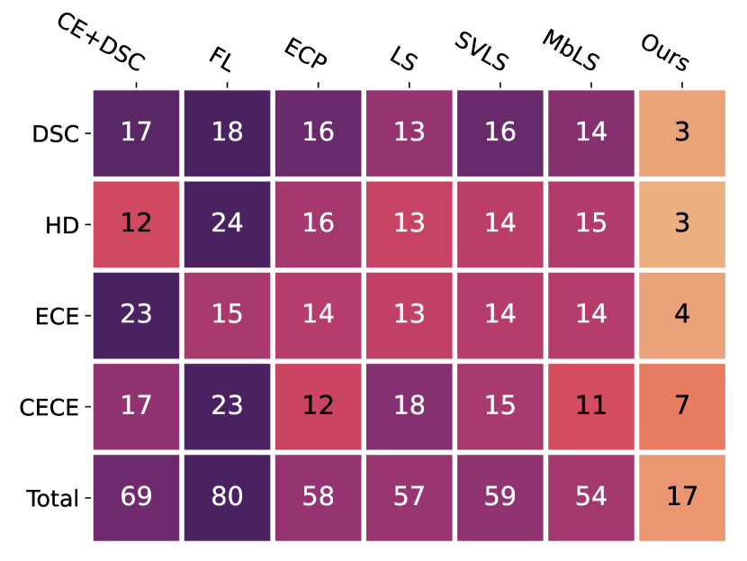
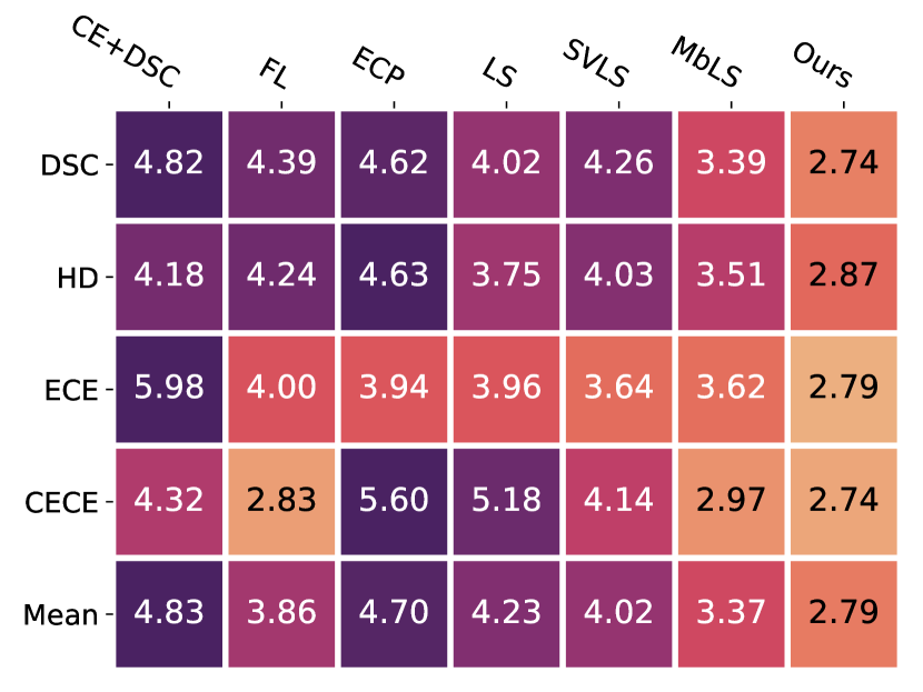
Figure 1: Sum-rank and mean-rank evaluation. Ranking of the different methods based on the sum-rank (left) and mean of case-specific (right) approaches. The lower the value, the better the performance.

Ablation studies. 1-Constraint over logits vs softmax. Recent evidence [11] suggests that imposing constraints on the logits presents a better alternative than its softmax counterpart. To demonstrate that this observation holds in our model, we present the results of our formulation when the constraint is enforced on the softmax distributions, i.e., replacing $\bf{l}$ by $\bf{s}$ (Table 2, top), which yields inferior results. 2-Choice of the penalty. To solve the unconstrained problem in Eq. 7, we can approximate the second term with a liner penalty, modeled as a ReLU function. Nevertheless, we can resort to other polynomial penalties, e.g., quadratic penalties, whose main difference stems from the more aggressive behavior of quadratic penalties over larger constraint violations. The results obtained when the linear penalty is replaced by a quadratic penalty are reported in Table 2 (middle). From these results, we can observe that, while a quadratic penalty could achieve better results in a particular dataset (e.g., ACDC or calibration performance on BraTS), a linear penalty yields more consistent results across datasets. 3-Patch size. For a fair comparison with SVLS, we used a patch of size 3 $\times$ 3 in our model. Nevertheless, we now investigate the impact of employing a larger patch to define the prior $\bm{\tau}$, whose results are presented in Table 2 (bottom). Even though a larger patch seems to bring comparable results in one dataset, the performance on the other two datasets is largely degraded, which potentially hinders its scalability to other applications. We believe that this is due to the higher degree of noise in the class distribution, particularly when multiple organs overlap, as the employed patch covers a wider region.

Table 2: Empirical results to motivate our methodological and technical choices.

	FLARE				ACDC				BraTS
	DSC	HD	ECE	CECE	DSC	HD	ECE	CECE	DSC	HD	ECE	CECE
Constraint on $\bf{s}$	0.862	5.14	0.043	0.030	0.840	2.66	0.068	0.071	0.802	8.28	0.145	0.104
L2-penalty	0.851	5.48	0.065	0.054	0.871	1.78	0.059	0.080	0.851	7.90	0.078	0.091
Patch size: 5 $\times$ 5	0.875	5.96	0.032	0.031	0.813	3.50	0.078	0.077	0.735	7.45	0.119	0.092

Impact of the prior. A benefit of the proposed formulation is that diverse priors can be enforced on the logit distributions. Thus, we now assess the impact of different priors $\bm{\tau}$ in our formulation (See Supplemental Material for a detailed explanation). The results presented in Table 3 reveal that selecting a suitable prior can further improve the performance of our model.

Table 3: Impact of using different priors ($\bm{\tau}$) in Eq. 7.

	FLARE				ACDC				BraTS
Prior $\bm{\tau}$	DSC	HD	ECE	CECE	DSC	HD	ECE	CECE	DSC	HD	ECE	CECE
Mean	0.868	4.88	0.033	0.031	0.854	2.55	0.048	0.061	0.850	5.78	0.112	0.097
Gaussian	0.860	5.40	0.033	0.032	0.876	2.92	0.042	0.053	0.813	7.01	0.140	0.106
Max	0.859	4.95	0.038	0.036	0.876	1.74	0.046	0.054	0.833	8.25	0.114	0.094
Min	0.854	5.42	0.034	0.033	0.881	1.80	0.040	0.053	0.836	7.23	0.104	0.092
Median	0.867	5.90	0.033	0.032	0.835	3.29	0.075	0.075	0.837	7.53	0.095	0.089
Mode	0.854	5.41	0.035	0.034	0.876	1.62	0.045	0.056	0.808	8.21	0.135	0.113

Magnitude of the logits. To empirically demonstrate that the proposed solution decreases the logit values, we plot average logit distributions across classes on the FLARE test set (Fig. 2). In particular, we first separate all the voxels based on their ground truth labels. Then, for each category, we average the per-voxel vector of logit predictions (in absolute value). We can observe that, compared to SVLS and MbLS, –which also imposes constraints on the logits–, our approach leads to much lower logit values, particularly compared to SVLS.

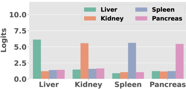
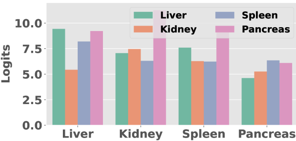
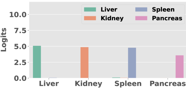
Figure 2: Distribution of logit values. From left to right: MbLS, SVLS and ours.

4 Conclusion

We have presented a constrained-optimization perspective of SVLS, which has revealed two important limitations of this method. First, the implicit constraint enforced by SVLS cannot be controlled explicitly. And second, the prior imposed in the constraint is directly derived from the Gaussian kernel used, which makes it hard to model. In light of these observations, we have proposed a simple alternative based on equality constraints on the logits, which allows to control the importance of the penalty explicitly, and the inclusion of any desirable prior in the constraint. Our results suggest that the proposed method improves the quality of the uncertainty estimates, while enhancing the segmentation performance.

Table 1: Additional details on the different datasets employed in our evaluation.

	Dataset splits			Classes
	Train	Val	Test
FLARE	240	40	80	(1) Liver, (2) Kidneys, (3) Spleen, (4) Pancreas
ACDC	70	10	20	(1) Left Ventricle (LV), (2) Right Ventricle (RV), (3) Myocardium (MYO)
BraTS	235	35	65	(1) Tumor Core (TC), (2) Enhancing Tumor (ET), (3) Whole Tumor (WT)

We provide the formulation of different metrics used for evaluation:

- Expectation Calibration Error (ECE). The ECE can be approximated as a weighted average of the absolute difference between the accuracy and confidence of each bin: $ECE=\sum_{i=1}^{M}\frac{|B_{i}|}{N}|A_{i}-C_{i}|$, where $M$ denotes the number of equispaced bins, $B_{i}$ denote the set of samples with confidences belonging to the $i^{th}$ bin, $A_{i}$ is the accuracy of the $i$-th bin, and it is computed as $A_{i}=\frac{1}{|B_{i}|}\sum_{j\in B_{i}}1(\hat{y_{j}}=y_{j})$, where 1 is the indicator function, $\hat{y_{j}}$, and $y_{j}$ are the predicted and ground-truth labels for the $j^{th}$ sample. Similarly, the confidence $C_{i}$ of the $i^{th}$ bin is computed as $C_{i}=\frac{1}{|B_{i}|}\sum_{j\in B_{i}}\hat{p}_{j}$, i.e. $C_{i}$ is the average confidence of all samples in the bin.

- Classwise ECE. The simple classwise extension of the ECE metric is defined as: $CECE=\sum_{i=1}^{M}\sum_{j=1}^{K}\frac{|B_{i,j}|}{N}|A_{i,j}-C_{i,j}|$, where $K$ is the number of classes, $B_{ij}$ denotes the set of samples from the $j^{th}$ class in the $i^{th}$ bin, $A_{i,j}=\frac{1}{|B_{i,j}|}\sum_{k\in B_{i,j}}1(j=y_{k})$ and $C_{i,j}=\frac{1}{|B_{ij}|}\sum_{k\in B_{i,j}}\hat{p}_{kj}$.

- Sum-rank. We follow the strategy followed in several MICCAI Challenges, e.g., MRBrainS [14], where the final ranking is given as the sum of individual ranking metrics: $r_{mc}$, where $r_{mc}$ ${R_{T}=\sum_{m=0}^{|M|}r_{m}}$, where $r_{m}$ is the rank of the segmentation model for the metric $m$ (mean).

-Mean case-rank. Furthermore, to account for the different complexities of each sample, we follow the mean-case-rank strategy, which has been employed in other MICCAI Challenges, e.g., [13]. We first compute the DSC, HD, ECE, and CECE values for each sample, and establish each method’s rank based on these metrics, separately for each case. Then, we compute the mean rank over all four evaluation metrics, per case, to obtain the method’s rank for that given sample. Finally, we compute the mean over all case-specific ranks to obtain the method’s final rank.

Let the $\mathbf{y}^{*}\in\mathbb{R}$ be the label encoding with the unique values $\{1,..K\}$ for one-hot labels $\mathbf{y}\in\mathbb{R}^{K}$. For each of the prior, the label $\mathbf{y}$ is updated to $\tilde{\mathbf{y}}\in\mathbb{R}^{K}$. Thus, for a pixel ${p}$ with patch $d=d_{1}\times d_{2}$, the following equations can be used to obtain the prior:

$$\textrm{Mean:}\quad\tilde{y}^{k}_{p}=\frac{1}{d}\sum_{i=1}^{d}y_{i}^{k}$$ (1)

$$\textrm{Gaussian:}\quad\tilde{y}^{k}_{p}=\frac{1}{|\sum_{i}^{d}w_{i}|}\sum_{i=1}^{d}y^{k}_{i}w_{i},$$ (2)

where $w_{i}$ is the Gaussian kernel.

$$\textrm{Max:}\quad\tilde{y}^{k}_{p}=\begin{cases}1,&\underset{d}{max}(y^{*k})==k\\ 0,&\textrm{otherwise}.\end{cases}$$ (3)

The priors pertaining to Min, Mode, Median can also be obtained by replacing Eq. 3 with respective to order statistics operation.

Table 2: Class-wise segmentation scores on FLARE, ACDC, and BraTS datasets.

	Region	CE+DSC		FL		ECP		LS		SVLS		MbLS		Ours
		DSC	HD	DSC	HD	DSC	HD	DSC	HD	DSC	HD	DSC	HD	DSC	HD
	Liver	0.942	7.60	0.942	7.54	0.953	7.41	0.952	8.50	0.951	7.72	0.941	7.18	0.954	6.04
	Kidney	0.941	2.43	0.942	2.16	0.950	2.05	0.947	1.76	0.947	1.84	0.937	2.49	0.952	1.84
	Spleen	0.867	3.70	0.875	9.09	0.887	3.98	0.905	4.62	0.879	6.40	0.868	4.73	0.900	4.26
	Pancreas	0.634	8.42	0.578	7.80	0.649	7.77	0.637	6.45	0.650	6.91	0.596	8.61	0.664	7.37
FLARE	Mean	0.846	5.54	0.834	6.65	0.860	5.30	0.860	5.33	0.857	5.72	0.836	5.75	0.868	4.88
	RV	0.799	3.10	0.580	9.37	0.751	4.93	0.796	3.34	0.791	2.89	0.812	2.59	0.837	3.02
	MYO	0.795	2.57	0.557	5.55	0.757	3.54	0.772	3.07	0.798	2.66	0.795	2.86	0.820	2.04
	LV	0.889	3.75	0.724	6.97	0.839	4.85	0.858	3.49	0.882	2.89	0.875	3.53	0.905	2.59
ACDC	Mean	0.828	3.14	0.620	7.30	0.782	4.44	0.809	3.30	0.824	2.81	0.827	2.99	0.854	2.55
	TC	0.730	5.73	0.799	7.80	0.749	7.53	0.773	5.16	0.744	7.56	0.803	4.88	0.804	3.98
	ET	0.746	8.27	0.854	10.02	0.790	11.31	0.807	10.23	0.783	9.22	0.821	10.85	0.854	6.58
	WT	0.855	6.88	0.889	9.19	0.884	7.28	0.879	7.94	0.877	8.55	0.889	8.09	0.893	6.78
BraTS	Mean	0.777	6.96	0.848	9.00	0.808	8.71	0.820	7.78	0.801	8.44	0.838	7.94	0.850	5.78

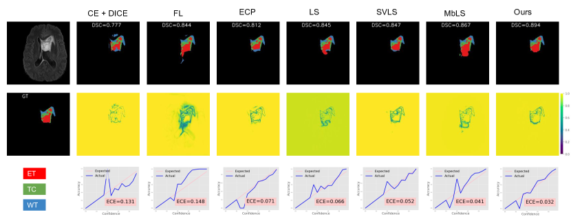
Figure 3: Qualitative results on BraTS dataset for different methods. In particular, we show the original image and the corresponding segmentation masks provided by each method (top row), the ground-truth (GT) mask followed by maximum confidence score of each method (middle row) and the respective reliability plots (bottom row). Methods from left to right: CE+DICE, FL, ECP, LS, SVLS, MbLS, Ours

.

References

- [1] Bakas, S., Akbari, H., Sotiras, A., Bilello, M., Rozycki, M., Kirby, J.S., Freymann, J.B., Farahani, K., Davatzikos, C.: Advancing the cancer genome atlas glioma MRI collections with expert segmentation labels and radiomic features. Scientific data 4(1), 1–13 (2017)
- [2] Bakas, S., Reyes, M., Jakab, A., Bauer, S., Rempfler, M., Crimi, A., Shinohara, R.T., Berger, C., Ha, S.M., Rozycki, M., et al.: Identifying the best machine learning algorithms for brain tumor segmentation, progression assessment, and overall survival prediction in the brats challenge. arXiv preprint arXiv:1811.02629 (2018)
- [3] Bernard, O., Lalande, A., Zotti, C., Cervenansky, F., Yang, X., Heng, P.A., Cetin, I., Lekadir, K., Camara, O., Ballester, M.A.G., et al.: Deep learning techniques for automatic MRI cardiac multi-structures segmentation and diagnosis: is the problem solved? IEEE TMI 37(11), 2514–2525 (2018)
- [4] Ding, Z., Han, X., Liu, P., Niethammer, M.: Local temperature scaling for probability calibration. In: ICCV (2021)
- [5] Gal, Y., Ghahramani, Z.: Dropout as a bayesian approximation: Representing model uncertainty in deep learning. In: ICML (2016)
- [6] Guo, C., Pleiss, G., Sun, Y., Weinberger, K.Q.: On calibration of modern neural networks. In: ICML (2017)
- [7] Islam, M., Glocker, B.: Spatially varying label smoothing: Capturing uncertainty from expert annotations. In: International Conference on Information Processing in Medical Imaging. pp. 677–688. Springer (2021)
- [8] Kingma, D.P., Ba, J.: Adam: A method for stochastic optimization. International Conference on Learning Representations (2015)
- [9] Kull, M., Perello Nieto, M., Kängsepp, M., Silva Filho, T., Song, H., Flach, P.: Beyond temperature scaling: Obtaining well-calibrated multi-class probabilities with dirichlet calibration. NeurIPS 32 (2019)
- [10] Lin, T.Y., Goyal, P., Girshick, R., He, K., Dollár, P.: Focal loss for dense object detection. In: CVPR (2017)
- [11] Liu, B., Ben Ayed, I., Galdran, A., Dolz, J.: The devil is in the margin: Margin-based label smoothing for network calibration. In: CVPR (2022)
- [12] Ma, J., Zhang, Y., Gu, S., Zhu, C., Ge, C., Zhang, Y., An, X., Wang, C., Wang, Q., Liu, X., Cao, S., Zhang, Q., Liu, S., Wang, Y., Li, Y., He, J., Yang, X.: Abdomenct-1K: Is abdominal organ segmentation a solved problem? IEEE Transactions on Pattern Analysis and Machine Intelligence (2021)
- [13] Maier, O., et al.: ISLES 2015 - a public evaluation benchmark for ischemic stroke lesion segmentation from multispectral MRI. Medical Image Analysis 35, 250–269 (2017)
- [14] Mendrik, A.M., Vincken, K.L., Kuijf, H.J., Breeuwer, M., Bouvy, W.H., De Bresser, J., Alansary, A., De Bruijne, M., Carass, A., El-Baz, A., et al.: MRBrainS challenge: online evaluation framework for brain image segmentation in 3T MRI scans. Computational intelligence and neuroscience (2015)
- [15] Menze, B.H., et al.: The multimodal brain tumor image segmentation benchmark (brats). IEEE Transactions on Medical Imaging 34(10), 1993–2024 (2015)
- [16] Mukhoti, J., Kulharia, V., Sanyal, A., Golodetz, S., Torr, P.H., Dokania, P.K.: Calibrating deep neural networks using focal loss. In: NeurIPS (2020)
- [17] Müller, R., Kornblith, S., Hinton, G.: When does label smoothing help? In: NeurIPS (2019)
- [18] Murugesan, B., Liu, B., Galdran, A., Ayed, I.B., Dolz, J.: Calibrating segmentation networks with margin-based label smoothing. Medical Image Analysis 87, 102826 (2023)
- [19] Naeini, M.P., Cooper, G., Hauskrecht, M.: Obtaining well calibrated probabilities using bayesian binning. In: Twenty-Ninth AAAI Conference on Artificial Intelligence (2015)
- [20] Ovadia, Y., Fertig, E., Ren, J., Nado, Z., Sculley, D., Nowozin, S., Dillon, J.V., Lakshminarayanan, B., Snoek, J.: Can you trust your model’s uncertainty? evaluating predictive uncertainty under dataset shift. In: NeurIPS (2019)
- [21] Pereyra, G., Tucker, G., Chorowski, J., Kaiser, Ł., Hinton, G.: Regularizing neural networks by penalizing confident output distributions. In: ICLR (2017)
- [22] Szegedy, C., Vanhoucke, V., Ioffe, S., Shlens, J., Wojna, Z.: Rethinking the inception architecture for computer vision. In: CVPR (2016)
- [23] Tomani, C., Gruber, S., Erdem, M.E., Cremers, D., Buettner, F.: Post-hoc uncertainty calibration for domain drift scenarios. In: CVPR (2021)
- [24] Zhang, J., Kailkhura, B., Han, T.: Mix-n-match: Ensemble and compositional methods for uncertainty calibration in deep learning. In: ICML (2020)