Interpretable Outlier Summarization

Abstract.

Outlier detection is critical in real applications to prevent financial fraud, defend network intrusions, or detecting imminent device failures. To reduce the human effort in evaluating outlier detection results and effectively turn the outliers into actionable insights, the users often expect a system to automatically produce interpretable summarizations of subgroups of outlier detection results. Unfortunately, to date no such systems exist. To fill this gap, we propose STAIR which learns a compact set of human understandable rules to summarize and explain the anomaly detection results. Rather than use the classical decision tree algorithms to produce these rules, STAIR proposes a new optimization objective to produce a small number of rules with least complexity, hence strong interpretability, to accurately summarize the detection results. The learning algorithm of STAIR produces a rule set by iteratively splitting the large rules and is optimal in maximizing this objective in each iteration. Moreover, to effectively handle high dimensional, highly complex data sets which are hard to summarize with simple rules, we propose a localized STAIR approach, called L-STAIR. Taking data locality into consideration, it simultaneously partitions data and learns a set of localized rules for each partition. Our experimental study on many outlier benchmark datasets shows that STAIR significantly reduces the complexity of the rules required to summarize the outlier detection results, thus more amenable for humans to understand and evaluate, compared to the decision tree methods.

1. Introduction

Motivation. Outlier detection is critical in enterprises, with applications ranging from preventing financial fraud in finance, and defending network intrusions in cyber security, to detecting imminent device failures in IoT.

To turn outliers into actionable insights, the users often expect an anomaly detection system to produce human understandable information to explain the detected outliers, e.g., by highlighting the features that contribute the most to the identified anomalies. Otherwise, the detected outliers are just a set of isolated data objects without any indication of their significance to the users. Further, outlier detection frequently returns a large number of outlier candidates. This raises the problem of how to best present results such that the users do not have to sift through a huge number of results to assess the validity of the outliers one by one.

If a system is able to summarize anomaly detection results into groups and explain why each group of objects is considered to be abnormal or normal, this will greatly reduce the effort of users in evaluating anomaly detection results.

State-of-the-Art. To the best of our knowledge, the problem of summarizing and interpreting outlier detection results is yet to be addressed. Scorpion (Wu and Madden, 2013) produces meaningful explanations for anomalies in aggregation queries when the ‘cause’ of an outlier is contained in its provenance. Similar to Scorpion, Cape (Miao et al., 2019) aims to explain the outliers in aggregation queries, but using the objects that counterbalance the outliers. Both works do not tackle the problem of summarizing outliers. Macrobase (Bailis et al., 2017) explains outliers by correlating them to some external attributes which are not used to detect anomalies such as location, time of occurrence, software version, etc. However, Macrobase only targets explaining the outliers captured by its default density-based outlier detector and does not generalize to other outlier detection methods.

In the broader field of interpretable AI, LIME (Ribeiro et al., 2016) explains the predictions of a classifier by learning a linear model locally around the prediction with respect to each testing object and pointing out the attributes that are most important to the prediction of the linear model. However, rather than use one model to represent a set of objects, LIME has to learn a linear model for each individual object. Therefore, using LIME to explain a large number of prediction results will be prohibitively expensive. Other methods (Ribeiro et al., 2018; Guidotti et al., 2018; Pedreschi et al., 2018) explain classification results in the similar way to LIME.

Challenges. Summarizing and interpreting outliers is challenging because of its nature. Outliers are phenomena that significantly deviate from the normal phenomena. In most cases the outliers tend to be very different from each other in their features. Therefore, they cannot be simply summarized based on their similarity in the feature space measured by some similarity function.

Proposed Approach. To meet the need of an effective outlier summarization and interpretation tool, we have developed STAIR. It produces a set of human understandable abstractions, each describing the common properties of a group of detection results. This allows the users to efficiently verify a large number of anomaly detection results and diagnose the root causes of the potential outliers by only examining a small set of interpretable abstractions.

Rule-based Outlier Summarization and Interpretation. STAIR leverages classical decision tree classification to learn a compact set of human understandable rules to summarize and explain the anomaly detection results. Using the results produced by an anomaly detection method as training data, STAIR learns a decision tree to accurately separate outliers and inliners in the training set. Each branch of the decision tree is composed of a set of data attributes with associated values that iteratively split the data. Therefore, it can be thought of as a rule that represents a subset of data sharing the same class (outlier or inlier) and that is easy to understand by humans.

Outlier Summarization and Interpretation-aware Objective. However, decision tree algorithms target maximizing the classification accuracy. Rules learned in this way do not necessarily have the properties desired by outlier summarization and interpretation. This is because when handling highly complex data sets, to minimize the classification errors, decision trees often have to be deep trees with many branches and hence produce a lot of complex rules which are hard for humans to understand. Although some methods like CART (Breiman et al., 1984) have been proposed to prune a learned decision tree in a post-processing step, they target avoiding overfitting and thus lifting the classification accuracy. They do not guarantee the simplicity of each rule.

To solve the above issues, we propose a new optimization objective customized to outlier summarization and interpretation. It targets producing the minimal number of rules that are as simple as possible, while still assuring the classification accuracy. However, the simplicity requirement of outlier summarization and interpretation conflicts with the accuracy requirement, while it is hard for the users to manually set an appropriate regularization term to balance the two requirements. STAIR thus introduces a learnable regularization parameter into the objective and relies on the leaning algorithm to automatically make the trade-off.

Rule Generation Algorithm. We then design an optimization algorithm to generate the summarization and interpretation-aware rules. Similar to the classic decision tree algorithms (Elaidi et al., 2018), STAIR produces a rule set by iteratively splitting the decision node. In each iteration, STAIR dynamically adjusts the regularization parameter to ensure that it is always able to produce a valid split which increases the objective. We prove that the regularization parameter and the rule split that STAIR learns in each iteration as a combination is optimal in maximizing the objective.

Localized Outlier Summarization and Interpretation. To solve the problem that one single decision tree with a small number of simple rules is not adequate to satisfy the accuracy requirement when handling high dimensional, highly complex data sets, we propose a localized STAIR approach, called L-STAIR. Taking data locality into consideration, L-STAIR divides the whole data set into multiple partitions and learns a localized tree for each partition. Rather than first partition the data and then learn the localized tree in two disjoint steps, L-STAIR jointly solves the two sub-problems. In each iteration, it optimizes the data partitioning and rule generation objectives alternatively and is guaranteed to converge to a partitioning that can be summarized with simple rules.

Contributions. The key contributions of this work include:

• To the best of our knowledge, STAIR is the first approach that summarizes the outlier detection results with human interpretable rules.

• We define an outlier summarization and interpretation-aware optimization objective which targets producing the minimal number of rules with least complexity, while still guaranteeing the classification accuracy.

• We design a rule generation method which is optimal in optimizing the STAIR objective in each iteration.

• We propose a localized STAIR approach which jointly partitions the data and produces rules for each local partition, thus scaling STAIR to high dimensional, highly complex data.

• Our extensive experimental study confirms that compared to other decision tree methods, STAIR significantly reduces the complexity and the number of rules required to summarize outlier detection results.

2. Preliminary: Decision Tree

In this section, we overview the decision tree classification problem and its classical learning algorithms.

Decision Tree Overview. Decision tree learning is a classical classification technique where the learned function could be represented by a decision tree. It classifies instances by sorting them down the tree from root to the leaf node, which could predict the label of this instance. Each node in the tree denotes the test of the specific attribute, and the instance is classified by moving down the tree branch from this node according to the value of the attribute in the given example.

Learning Algorithms. Most algorithms learn the decision trees in a top-town, greedy search manner such as ID3 (Quinlan, 1986) and its successor C4.5 (Quinlan, 1993). The basic algorithm, ID3, will run a statistical test on choosing the instance attribute to determine how well it could classify the data points. From the root node, the algorithm will find the best attribute to form branches and then put all the training examples into the corresponding child nodes. It then repeats this entire process using the training data associated with the child nodes to select the appropriate attribute and value for the current node and form new branches from the child nodes.

Information Gain-based Statistical Test. There are several strategies for the statistical test in each step. One of the most popular tests is information gain, which measures how well a given attribute could separate the training examples. Before giving the precise definition of information gain, we need to give the definition of entropy first. Given a data collection $S$, containing positive and negative examples, the entropy of $S$ is:

(1) $$Entropy(S)=-p_{+}\log_{2}p_{+}-p_{-}\log_{2}p_{-}$$

where $p_{+}$ and $p_{-}$ are the proportion of positive and negative examples in $S$, respectively.

Next, we give the formulation of the information gain of an attribute $A$ with split value $v$, relative to a collection of examples $S$:

(2) $$Gain(S,A,v)=Entropy(S)-\sum_{b\in Branches}\frac{|S_{b}|}{|S|}Entropy(S_{b})$$

where Branches contains two branches, each of which has the training examples with attribute $A$ smaller or larger than the value $v$, respectively. $S_{b}$ refers to the collection of examples from branch $b$. The learning algorithm iteratively splits nodes and forms branches by maximizing Eq. 2 at each step.

Learning the decision tree in this way is equivalent to maximizing the global objective:

(3) $$\max\sum_{l\in L}n_{l}(1-Entropy(S_{l}))$$

where $S_{l}$ represents the collection of training examples in the leaf node $l$ and $n_{l}$ represents the number of examples falling into node $l$.

3. Rule-based Summarization and Interpretation

In this section, we first give the definition of rule and then explain why rules are good at summarizing and interpreting outlier detection results.

Definition 3.0.

Given a data set $\mathbb{D}$ in a N-dimensional feature space $\mathit{[x_{1},x_{2},\cdots,x_{N}]}$, a Rule $R_{i}$ is defined as $\mathit{R_{i}=(a_{1}\leq x^{i}_{1}\leq b_{1})}$ $\land$ $\mathit{(a_{2}\leq x^{i}_{2}\leq b_{2})}$, $\cdots$, $\land$ $\mathit{(a_{j}\leq x^{i}_{j}\leq b_{j})}$, $\cdots$, $\land$ $\mathit{(a_{L}\leq x^{i}_{L}\leq b_{L})}$. $\forall$ clause $\mathit{(a_{j}\leq x^{i}_{j}\leq b_{j})}$ of $R_{i}$, $x^{i}_{j}$ corresponds to one attribute $x_{j}$ $\in$ $\{x_{1},x_{2},\cdots,x_{N}\}$; $a_{j}$ and $b_{j}$ ($a_{j}$ $<$ $b_{j}$) fall in the domain range of attribute $x_{j}$. $L$ indicates the number of attributes in rule $R_{i}$, or the length of $R_{i}$.

By Def. 3.1, a rule $R_{i}$ corresponds to a conjunction of domain value intervals, each with respect to some attribute $x_{j}$. Rule $R_{i}$ covers a data subset $\mathbb{D}_{i}$ $\subseteq$, where $\forall$ object $d_{i}$ $\in$ $\mathbb{D}_{i}$, the attributes of object $d_{i}$ fall into the corresponding interval.

In the decision tree model (Safavian and Landgrebe, 1991), each branch corresponds to one rule. Fig. 1(a) shows a toy decision tree $T_{i}$ learned from a 2-dimensional data set $\mathbb{D}$. $T_{i}$ classifies the objects in $\mathbb{D}$ into outliers and inliers. It has three branches, corresponding to 3 rules: $\mathit{R_{1}=(-2\leq x_{1}\leq 2)}$, $\mathit{R_{2}=(x_{1}>2)}$, and $\mathit{R_{3}=(x_{1}<-2)}$. All rules only contain one attribute $x_{1}$. Rules $R_{2}$ and $R_{3}$ are lower bounded or upper bounded only. Thus the length of these rules is one.

Note the length of a rule is not equivalent to the depth of the tree. The depth of the decision tree in Figure 1(b) is two, while the lengths of the three rules are all one. Even if the decision tree gets deeper, the lengths of the rules could still be small. This is because a decision tree could use one attribute multiple times on one single branch (rule).

These rules classify the whole data set into three different partitions. Rule $R_{1}$ covers all inliers in $\mathbb{D}$, while both $R_{2}$ and $R_{3}$ represent outliers.

Rules effectively summarize and interpret the outliers and inliers in the data. The merit is twofold. First, each rule covers a set of inliers or outliers. Therefore, rather than exhaustively evaluating the large number of outliers or inliers one by one, the users now only have to evaluate a small number of rules, thus saving huge amount of human efforts. Second, the rules are human interpretable, helping the users easily understand why an object is considered as outlier or inlier and identify the root cause of the outliers. For example, rules $R_{2}$ and $R_{3}$ intuitively tell users that some objects are abnormal because their $x_{1}$ values are too large or too small.

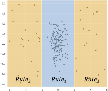
(a) Rules

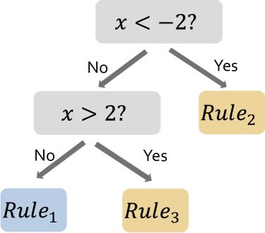
(b) Decision Tree

Figure 1. Example of rules and decision tree. The blue partition covered by $Rule_{1}$ represents inliers, while the brown partitions covered by $Rule_{2}$ and $Rule_{3}$ represent outliers.

4. The optimization objective of Rules Generation

4.1. The Insufficiency of Classic Decision Trees

Intuitively, to produce rules effectively summarizing and interpreting the outlier detection results, we could directly apply the classical decision tree algorithms such as ID3 (Elaidi et al., 2018). That is, we use the output of the outlier detection method as ground truth labels to train a decision tree model and then extract rules from the learned decision tree.

However, decision tree algorithms target producing rules that maximize the classification accuracy. The rules learned in this way do not necessarily have the desired properties when used in outlier summarization and interpretation, for the following reasons:

First, they may produce rules that contain many attributes and thus are too complicated for humans to evaluate. For examples, humans can easily understand and reason on a rule with a couple of attributes such as the rules in Fig. 1, while it will be much harder for the humans to obtain any meaningful information from a complicated rule with many attributes. For instance, the rule with 20 attributes $a_{1}\leq x_{1}\leq b_{1},\cdots,a_{20}\leq x_{20}\leq b_{20}$ will be almost impossible for human to understand.

Second, to maximize the classification accuracy they may produce many rules. However, to reduce the human evaluation efforts, ideally we want to produce as few rules as possible.

The above situations could happen when handling highly complex data sets which often require a deep tree with many branches.

4.2. Summarization and Interpretation-aware Objective

To address the above concerns, we design an optimization objective customized to outlier summarization and interpretation. It targets producing the minimal number of rules that are as simple as possible, while still guaranteeing the classification accuracy. The objective is composed of two sub-objectives, namely length objective and entropy objective.

Length Objective. To minimize the number of the rules as well as bounding the complexity of each rule, we first introduce an objective with respect to the lengths of the rules in rule set $\mathcal{R}$:

(4) $$\min_{\mathcal{R}}\mathcal{L}(\mathcal{R}), \textrm{ where }\mathcal{L}(\mathcal{R})=\sum_{r_{i}\in\mathcal{R}}L(r_{i})$$

s.t. $$L(r_{i})\leq L_{m}$$

In Eq. 4, $\mathcal{R}$ denotes a rule set. $L(r_{i})$ denotes the length of a rule $r_{i}$ in $\mathcal{R}$. $L_{m}$ is the predefined maximal length of each rule that the users allow. Essentially, the total length of all rules represent the complexity of the learn model. Minimizing it will effectively reduce the number of rules, while at the same time simplifying each rule.

Entropy Objective. To maximize the classification accuracy of the derived model, we adopt the entropy-based optimization objective from the classical decision tree algorithms (Elaidi et al., 2018), i.e. ID3 and C4.5, as illustrated in Sec. 2.

(5) $$\max_{\mathcal{R}}\mathcal{S}(\mathcal{R}),\textrm{ where }\mathcal{S}(\mathcal{R})=\sum_{r_{i}\in\mathcal{R}}n_{r_{i}}E(r_{i})$$

In Equation 5, $E(r_{i})$ corresponds to $\mathit{1-Entropy(r)}$. Maximizing Eq. 5 effectively maximizes the classification accuracy.

Combing Eq. 5) and Eq. 4), our summarization and interpretation-aware objective (Eq. 7) maximizes the classification accuracy, while at the same time minimizing the total length of the rules.

(6) $$\max_{\mathcal{R}}\mathcal{S}(\mathcal{R})=\frac{\sum_{r_{i}\in\mathcal{R}}n_{r_{i}}E(r_{i})}{\sum_{r_{i}\in\mathcal{R}}L(r_{i})}$$

$$\textrm{ s.t. }L(r_{i})\leq L_{m},F1(\mathcal{R})>F1_{m}$$

where $L_{m}$ corresponds to the maximal length of a rule that the users allow, while $F1_{m}$ is a predefined requirement on classification accuracy which is measured by F1 score in the case of outlier detection. Optimization Issue. However, in practice we observed that this objective caused issues in the optimization process. Maximizing the entropy objective typically will lead to more complex rules and in turn the increase of the length objective. However, the length objective often increases faster than the entropy objective. Therefore, the overall objective (Eq. 6) tends to stop increasing in a few iterations.

Final Objective: Introducing a Stabilizer. To solve this problem, we introduce a stabilizer $M$ into the length objective – the denominator of Eq. 6:

(7) $$\max_{\mathcal{R},M}\mathcal{S}(\mathcal{R,M})=\frac{\sum_{r_{i}\in\mathcal{R}}n_{r_{i}}E(r_{i})}{\sum_{r_{i}\in\mathcal{R}}L(r_{i})+M}$$

$$\textrm{ s.t. }L(r_{i})\leq L_{m},F1(\mathcal{R})>F1_{m}$$

The stabilizer $M$ mitigates the impact of the quickly increasing length objective. It ensures that the length objective does not dominate our summarization and interpretation-aware objective. Intuitively, in the extreme case of setting $M$ to an infinite large value, the increase of the total rule length is negligible to the objective. Now maximizing Eq. 7 in fact is equivalent to the traditional entropy-based decision tree.

Auto-learning Stabilizer M. An appropriate value of $M$ is critical to the quality of the learned rules. However, relying on the users to manually tune it is difficult. First, $M$ can be any positive value and thus has infinite number of options. Second, ideally $M$ should dynamically change to best fit the evolving rule set produced in the iterative learning process. Therefore, rather than make it a hyper-parameter, $M$ is a learnable parameter in our objective function Eq. 7.

5. STAIR: Rule Generation Method

This section introduces our SummarizaTion And Interpretation-aware Rule generation method (STAIR). Similar to the classic decision tree algorithms (Elaidi et al., 2018), STAIR produces a rule set by iteratively splitting the decision node. We prove that in each iteration STAIR is optimal in maximizing our objective in Eq. 7.

Below we first give the overall process of STAIR:

1. Initialize the stabilizer $M$ in Eq. 7 to zero;

2. Increase the value of $M$;

3. Find a node to split that could increase the objective in Eq. 7; go to step 2.

In short, STAIR iteratively increases the value of $M$ and splits the nodes. Next, we first show that the value of $M$ is critical to the performance of STAIR and then introduce a method to calculate the optimal value of $M$ at each iteration.

5.1. The Value of M Matters

Given a rule set $\mathcal{R}$, splitting a node $n$ is equivalent to dividing one rule $r$ in $\mathcal{R}$ into two rules $r_{1}$ and $r_{2}$, where $r_{1}$ and $r_{2}$ end at the two child nodes of node $n$ correspondingly. Given an $M$ and a rule set $\mathcal{R}$, we say a split $\mathit{sp(\mathcal{R},M)}$ is valid if $\mathit{\mathcal{S}(\mathcal{R}\backslash\{r\}\cup\{r_{1},r_{2}\},M)>\mathcal{S}(\mathcal{R},M)}$. That is, a valid split will increase the objective defined in Eq. 7. For the ease of presentation, we use $\mathit{\mathcal{S}(\mathcal{R}^{\prime},M)}$ to denote $\mathit{\mathcal{S}(\mathcal{R}\backslash\{r\}\cup\{r_{1},r_{2}\},M)}$

Next, we show the smallest $M$ that could produce a valid split is optimal in maximizing Eq. 7.

Theorem 5.1.

Monotonicity Theorem. Given a rule set $\mathcal{R}$, if $M_{a}$ $>$ $M_{b}$, then $\mathit{\mathcal{S}(\mathcal{R}^{\prime}_{a},M_{a})}$ is guaranteed to be smaller than $\mathit{\mathcal{S}(\mathcal{R}^{\prime}_{b},M_{b})}$, where $\mathit{\mathcal{R}^{\prime}_{a}}$, $\mathcal{R}^{\prime}_{b}$ denotes the rule set produced by a valid split on $\mathcal{R}$ that maximizes the objective given $M_{a}$ or $M_{b}$.

Proof.

Because $M_{a}>M_{b}$, we have:

$$S(\mathcal{R}^{\prime}_{a},M_{a}) =\frac{\sum_{r\in\mathcal{R}^{\prime}_{a}}n_{r}E(r)}{\sum_{r\in\mathcal{R^{\prime}}_{a}}L(r)+M_{a}}$$

(8) $$<\frac{\sum_{r\in\mathcal{R}^{\prime}_{a}}n_{r}E(r)}{\sum_{r\in\mathcal{R}^{\prime}_{a}}L(r)+M_{b}}=S(\mathcal{R}^{\prime}_{a},M_{b})$$

Because $\mathcal{R}^{\prime}_{b}$ corresponds to the best split given $M_{b}$, we obtain:

(9) $$S(\mathcal{R}^{\prime}_{a},M_{b})\leq S(\mathcal{R}^{\prime}_{b},M_{b})$$

From Eq. 5.1 and Eq. 9, we have:

(10) $$\mathcal{S}(\mathcal{R}^{\prime}_{a},M_{a})<\mathcal{S}(\mathcal{R}^{\prime}_{b},M_{b})$$

This concludes our proof. ∎

5.2. Calculating the Optimal $M$

By Theorem 5.1, to maximize the objective at each iteration, it is necessary to search for the smallest value of $M$ that could produce a valid split. Intuitively we could find the optimal $M$ by gradually increasing the value of $M$ at a fixed step size. However, this is neither effective nor efficient, because it is hard to set an appropriate step size. If it is too large, STAIR might miss the optimal $M$. On the other hand, if the step size is too small, STAIR risks to incur many unnecessary iterations not producing any valid splits.

To solve the above problem, we introduce a method which uses the concept of boundary stabilizer to directly calculate the optimal $M$. Moreover, the best splitting is discovered as the by-product of this step.

We use $M_{o}$ to denote the optimal $M$. Because $M_{o}$ is the smallest $M$ that could produce a valid split, then $\forall r_{0}$ and $\forall r_{1},r_{2}$, where $r_{1}$ and $r_{2}$ represent the rules produced by splitting rule $r_{0}$, Eq. 11 holds:

(11) $$\mathcal{S}(\mathcal{R},M)>\mathcal{S}(\mathcal{R}\backslash\{r_{0}\}\cup\{r_{1},r_{2}\},M),\forall M<M_{o}$$

Boundary Stabilizer M. To compute $M_{o}$, we first define a boundary $M$ denoted as $M_{b}$ which makes Equation 12 hold:

(12) $$\mathcal{S}(\mathcal{R},M_{b})=\mathcal{S}(\mathcal{R}\backslash\{r_{0}\}\cup\{r_{1},r_{2}\},M_{b})$$

By Eq. 12, setting the $M$ to $M_{b}$ will produce a split that does not change the objective. That is, under $M_{b}$ no valid split will increase the objective. But there exists a split that does not decrease the objective. So $M_{b}$ is called the boundary $M$,

We then expand Eq. 12 as follows:

$$\frac{\sum_{r\in\mathcal{R}\backslash\{r_{0}\}}n_{r}E(r)+n_{r_{0}}E(r_{0})}{\sum_{r\in\mathcal{R}\backslash\{r_{0}\}}L(r)+L(r_{0})+M_{b}}$$

(13) $$=\frac{\sum_{r\in\mathcal{R}\backslash\{r_{0}\}}n_{r}E(r)+n_{r_{1}}E(r_{1})+n_{r_{2}}E(r_{2})}{\sum_{r\in\mathcal{R}\backslash\{r_{0}\}}L(r)+L(r_{1})+L(r_{2})+M_{b}}$$

We define $A=\sum_{r\in\mathcal{R}\backslash\{r_{0}\}}n_{r}E(r),B=\sum_{r\in\mathcal{R}\backslash\{r_{0}\}}L(r)$, and $A_{0}=\sum_{r\in\mathcal{R}}n_{r}E(r),B_{0}=\sum_{r\in\mathcal{R}}L(r)$, then Eq. 13 could be rewritten as:

(14) $$\frac{A+n_{r_{0}}E(r_{0})}{B+L(r_{0})+M_{b}}=\frac{A+n_{r_{1}}E(r_{1})+n_{r_{2}}E(r_{2})}{B+L(r_{1})+L(r_{2})+M_{b}}$$

Then after some mathematical transformation, we obtain:

$$M_{b}( n_{r_{1}}E(r_{1})+n_{r_{2}}E(r_{2})-n_{r_{0}}E(r_{0}))$$

$$=n_{r_{0}}E(r_{0})(L(r_{1})+L(r_{2}))+A(L(r_{1})+L(r_{2})-L(r_{0}))$$

$$-B(n_{r_{1}}E(r_{1})+n_{r_{2}}E(r_{2})-n_{r_{0}}E(r_{0}))$$

(15) $$-(n_{r_{1}}E(r_{1})+n_{r_{2}}E(r_{2}))L(r_{0})$$

Denoting $\mathit{\Delta L=L(r_{1})+L(r_{2})-L(r_{0})}$ and $\mathit{\Delta E=n_{r_{1}}E(r_{1})+n_{r_{2}}E(r_{2})-n_{r_{0}}E(r_{0})}$, we simplify Eq. 5.2 to:

$$M_{b}\Delta E =n_{r_{0}}E(r_{0})(L(r_{1})+L(r_{2}))+A\Delta L-B\Delta E$$

$$-(n_{r_{1}}E(r_{1})+n_{r_{2}}E(r_{2}))L(r_{0})$$

$$=A\Delta L-B\Delta E+n_{r_{0}}E(r_{0})\Delta L-L(r_{0})\Delta E$$

(16) $$=(A+n_{r_{0}}E(r_{0}))\Delta L-(B+L(r_{0}))\Delta E$$

(17) $$M_{b} =A_{0}\frac{\Delta L}{\Delta E}-B_{0},\forall r_{0}\in\mathcal{R},\forall r_{1},r_{2}$$

$\forall M>M_{b}$, with the same $r_{0}$ and $r_{1},r_{2}$ in Eq. 12, Eq. 5.2 becomes:

$$M( n_{r_{1}}E(r_{1})+n_{r_{2}}E(r_{2})-n_{r_{0}}E(r_{0}))$$

$$>n_{r_{0}}E(r_{0})(L(r_{1})+L(r_{2}))+A(L(r_{1})+L(r_{2})-L(r_{0}))$$

$$-B(n_{r_{1}}E(r_{1})+n_{r_{2}}E(r_{2})-n_{r_{0}}E(r_{0}))$$

(18) $$-(n_{r_{1}}E(r_{1})+n_{r_{2}}E(r_{2}))L(r_{0})$$

Note that with expanding $r_{0}$ to $r_{1},r_{2}$, the entropy of the rules must be lower, which means $n_{r_{1}}E(r_{1})+n_{r_{2}}E(r_{2})-n_{r_{0}}E(r_{0})>0$.

Then from Eq. 5.2 to Eq. 12, we may easily obtain Eq. 19 from Eq. 5.2:

(19) $$\mathcal{S}(\mathcal{R},M)<\mathcal{S}(\mathcal{R}\backslash\{r_{0}\}\cup\{r_{1},r_{2}\},M),\forall M>M_{b}$$

That is, an $M$ larger than $M_{b}$ is guaranteed to produce a valid split – splitting rule $r_{0}$ to $r_{1}$ and $r_{2}$.

Calculating Optimal M. According to the Monotonicity theorem (Theorem 5.1), a smallest $M$ is the best in maximizing the objective. Therefore, STAIR can directly calculate $M_{o}$ using Eq. 20:

(20) $$M_{o}>\min_{\Delta L/\Delta E}A_{0}\frac{\Delta L}{\Delta E}-B_{0},\forall r_{0}\in\mathcal{R},\forall r_{1},r_{2}$$

That is, STAIR first finds a rule $r_{0}$ from $\mathcal{R}$ that after split into two rules, produces the smallest $\frac{\Delta L}{\Delta E}$. STAIR then sets $M_{o}$ as a value larger than $\frac{\Delta L}{\Delta E}$ - $B_{0}$. In this way, STAIR successfully calculates the optimal $M$ and finds the best split in one step, making its learning process effective yet efficient.

5.3. STAIR Learning Algorithm

Input: Training data $X$, $F1$ score threshold $F1_{m}$

Output: The target rule set.

1 Initialize $M$ to be zero;

2 Initialize the min heap $H$ to contain only the root node;

3 Set the rule set $\mathcal{R}=\{r_{0}\}$;

4 $A_{0}=nE(r_{0}),B_{0}=0$;

5 while True do

6       extract from $H$ a rule $r_{0}$ which has the minimal $\frac{\Delta L}{\Delta E}$ ;

7       Set $M=A_{0}(\frac{\Delta L}{\Delta E})_{r_{0}}-B_{0}$;

8      

9      while the minimal $(\frac{\Delta L}{\Delta E})_{r_{0}}$ from $H$ $\leq\frac{M+B_{0}}{A_{0}}$ do

10             Extract rule $r_{0}$ with the minimal $(\frac{\Delta L}{\Delta E})_{r_{0}}$ from $H$;

11             Split $r_{0}$ into $r_{1},r_{2}$ ;

12             Insert $r_{1},r_{2}$ into $\mathcal{R}$ and $H$; Maintain the heap $H$ according to $(\frac{\Delta L}{\Delta E})_{r_{1}}$ and $(\frac{\Delta L}{\Delta E})_{r_{2}}$;

13             $A_{0}\leftarrow A_{0}+E(r_{1})+E(r_{2})-E(r)$;

14             $B_{0}\leftarrow B_{0}+L(r_{1})+L(r_{2})-L(r)$;

15            

16       end while

17      Calculate the $F1$-score of the current rule set as $F1(\mathcal{R})$;

18       if $F1(\mathcal{R})>F1_{m}$ then

19             Break;

20      

21 end while

Algorithm 1 Learning Algorithm of STAIR

Algorithm 1 shows the learning process of STAIR. It starts with initializing $M$ as 0 (Line 1) and uses a min heap structure $H$ to keep all nodes. Similar to the decision tree algorithms, it initializes $H$ to contain only the root node (Line 2). It then sets the rule set $\mathcal{R}$ to contain only one rule $r_{0}$ corresponding to the root node (Line 3). By default, rule $r_{0}$ classifies all training samples as inliers. Then based on Eq. 20, STAIR iteratively extracts a rule $r_{0}$, calculates $(\frac{\Delta L}{\Delta E})$, updates M, and splits $r_{0}$ into two rules $r_{1}$ and $r_{2}$. After each split, it calculates $(\frac{\Delta L}{\Delta E})$ with respect to $r_{1}$/$r_{2}$, refreshes the rule set $\mathcal{R}$ and min heap $H$, and updates $A_{0}$ and $B_{0}$ accordingly. The learning process will terminate when the following conditions hold: (1) the accuracy reaches the requirement specified by users; and (2) the $\mathit{\mathcal{S}(\mathcal{R},M)}$ does not increase in a few iterations.

Complexity Analysis. Compared to the classical decision tree algorithms, the additional overhead that STAIR introduces is negligible. In each iteration, STAIR extracts the rule $r_{0}$ from min heap $H$ and inserts into $H$ the new rules. Assume there are $n$ nodes in the tree. Because the complexity of min heap’s retrieve and insert operations is $O(\log n)$, the additional complexity is $O(n\log n)$.

6. Localized STAIR: Data Partitioning & Rule Generation

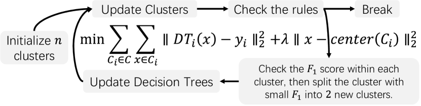
Figure 2. The Localized STAIR

As shown in our experiments (Sec. 7), although in general STAIR performs much better than the classical decision tree algorithms in producing summarization and interpretation friendly rules, its performance degrades quickly on high dimensional, highly complex data sets, for example on the SpamBase data set which has 57 attributes. This is because a single decision tree with a small number of simple rules is not powerful enough to model the complex distribution properties underlying these data sets.

To solve this problem, we propose a localized STAIR approach, so called L-STAIR. L-STAIR divides the whole data set into multiple partitions and learns a tree model for each partition. Taking the data locality into consideration, L-STAIR produces data partitions where the data in each partition share the similar statistical properties, while different partitions show distinct properties. L-STAIR thus is able to produce localized, simple rules that effective summarize and explain each data partition.

Next, we first introduce the objective of L-STAIR in Sec. 6.1 and then give the learning algorithm in Sec. 6.2.

6.1. Joint Optimization of Data Partitioning and Rule Generalization

Intuitively, L-STAIR could produce the localized rules in two disjoint steps: (1) partitioning data using the existing clustering algorithms such as k-means (Kanungo et al., 2002) or density-based clustering (Ester et al., 1996); (2) directly applying STAIR on each data partition one by one. However, this two steps solution is sub-optimal in satisfying our objective, namely producing minimal number of interpretable rules that are as simple as possible to summarize the outlier detection results. This is because the problems of data partitioning and rule generation are highly dependent on each other. Clearly, rule generation relies on data partitioning. To generate localized rules, the data has to be partitioned first. However, on the other hand, without taking the objective of rule generation into consideration, clustering algorithm does not necessarily yield data partitions that are easy to summarize with simple thus interpretable rules. Therefore, L-STAIR solves the two sub-problems of data partitioning and rule generation jointly.

To achieve this goal, in addition to the summarization and interpretation-aware objective (Eq. 6) defined in Sec. 4.2, L-STAIR introduces a partitioning objective composed of error objective and locality objective.

Error Objective. We denote the partitions of a dataset as $\mathcal{C}=\{C_{i}\}_{i=1}^{n}$, where $n$ is the number of partitions and $C_{i}$ represents the $i$th partition. $DT_{i}$ denotes the decision tree learned for a data partition $C_{i}$. Decision tree $DT_{i}$ produces a prediction with respect to each object $x$ in data partition $C_{i}$, denoted as $\mathit{DT_{i}(x)}$.

Next, in Eq. 21 we define an error metric to measure how good a decision tree $\mathit{DT_{i}}$ fits the data in $C_{i}$:

(21) $$\sum_{x\in C_{i}}||DT_{i}(x)-y_{i}||_{2}^{2}$$

To ensure the classification accuracy, L-STAIR targets minimizing this error metric with respect to all data partitions, which yields the error objective:

(22) $$\min_{\mathcal{C}}\sum_{C_{i}\in\mathcal{C}}\sum_{x\in C_{i}}||DT_{i}(x)-y||_{2}^{2}$$

where $y$ indicates the ground truth label of object $x$.

Locality Objective. Although using the above error objective to learn the data partitioning and the corresponding decision trees will effectively minimize the overall classification with respect to the whole dataset, the data partitions produced in this way do not preserve the locality of each data partition. Potentially one rule could cover a set of data objects that are scattered across the whole data space, thus is not amenable for human to understand. As shown in Figure 3, when the locality is preserved, the rules are constrained within each cluster. This means there is no overlapping between the rules. Then the generated rules will be easier to understand.

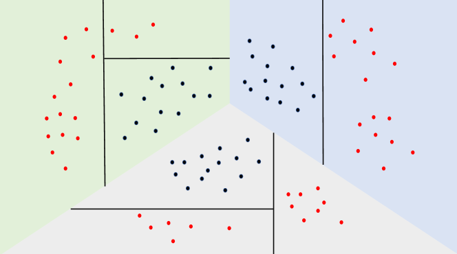
Figure 3. The intuition of locality: The black points are inliers and the red ones are outliers. The backgrounds with different colors refer to three clusters, while the straight lines in each cluster represent the rules.

Therefore, to ensure the data locality of each partition, we introduce the locality objective:

(23) $$\min_{\mathcal{C}}\sum_{C_{i}\in\mathcal{C}}||x-center(C_{i})||_{2}^{2}$$

Optimizing on the locality objective enforces the objects within each partition to be close to each other, similar to the objective of clustering such as k-means.

The Final L-STAIR Objective. Combining Eq. 23 and Eq. 22 together leads to the final partitioning objective:

(24) $$\min_{\mathcal{C}}\mathcal{L}_{L-STAIR}(\mathcal{C})=\sum_{C_{i}\in\mathcal{C}}\sum_{x\in C_{i}}||DT_{i}(x)-y||_{2}^{2}+\lambda||x-center(C_{i})||_{2}^{2}$$

Eq. 24 uses $\lambda$ ($\mathit{0<\lambda<1}$) to balance these two objectives. Setting the $\lambda$ to a small value will give error objective higher priority.

6.2. L-STAIR Learning Algorithm

L-STAIR jointly optimizes the partitioning objective (Eq. 24) and the summarization and interpretation-aware objective (Eq. 6) in an iterative manner. As shown in Figure 4, L-STAIR starts with initializing $n$ data partitions by using some clustering algorithms such as k-means in our implementation. Then we apply the STAIR algorithm introduced in Sec. 5.3 to learn one summarization and interpretation-aware decision tree for each initial partition. Next, it iteratively updates the partitions and thereafter builds the decision trees correspondingly. During this process, L-STAIR dynamically modifies the number of partitions based on the classification accuracy of each individual decision tree, making the number of partitions self-adaptive to the data, as further illustrated in Sec. 6.3. Similar to our original STAIR approach, the learning process of L-STAIR terminates after the overall classification accuracy with respect to the whole data set is above the threshold $F1_{m}$ and the optimization objective does not improve anymore in a few iterations.

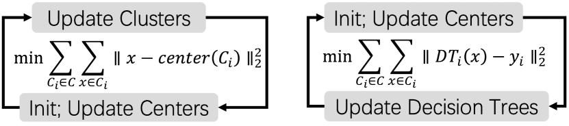
Figure 4. The correlation between our algorithm and the K-means algorithm

Input: Training data $X$, cluster number $n$ for initialization, $F_{1}$ score threshold $F_{1m}$

Output: Clusters $\mathcal{C}$ and decision tree for each cluster $DT_{i}$, $i\in\{1,\cdots,|\mathcal{C}|\}$

1 Initialize $n$ clusters using K-means;

2 while True do

3       Build $n$ new decision trees $DT_{i}$, $i=\{1,\cdots,n\}$ using the algorithm introduced in Section 5.3 for $n$ clusters;

4       Update the clusters $\mathcal{C}$ according to the objective Eq.(24);

5       Remove empty clusters;

6       Calculate the $F_{1}$ score of the predictions made by the MDTs(the rules), and denote it as $f_{1}$;

7       if $f_{1}>F_{1m}$ then

8            break;

9       Check the $F_{1}$ score within each cluster, split each of the clusters with too small $F_{1}$ scores to $n$ new clusters using K-means algorithm.

10 end while

Algorithm 2 L-STAIR learning algorithm

6.3. Dynamically Adjusting the Number of Partitions

As shown in Algorithm 2, L-STAIR uses the hyperparmeter $n$ to specify the number of partitions and initialize each data partition accordingly. It is well known that in many clustering algorithms such as k-means the number of clusters is a critical hyper-parameter which determines the quality of data partitioning; and it is hard to tune in many cases (Fu and Perry, 2020). L-STAIR does not rely on an appropriate $n$ to achieve good performance, because L-STAIR allows the users to set a small $n$ initially and then dynamically adjusts it in the learning process.

Producing New Partitions. L-STAIR will produce new partitions by splitting some partitions that are too complicated to summarize and explain with simple rules. The partition is said to be too complicated when the obtained $F1$-score on it is not good enough, more specifically lower than $F1_{m}$. This indicates that simple rules could not fully explain this partition. After identifying a complicated partition, L-STAIR uses k-means again to split it into two partitions, then build one decision tree for each new partition.

Removing Partitions. L-STAIR identifies the redundant partitions as those bearing large similarity to others such that merging them into other partitions do not degrade the partitioning objective. After identifying redundant partitions, L-STAIR will discard them and reassign their data points to other partitions.

Our experiments (Table 3, Sec. 7.5) on 10 datasets show that by starting with a small $n$ L-STAIR is always able to produce good results.

6.4. Convergence Analysis

We theoretically show that L-STAIR could converge. We establish this conclusion by showing that each step in Algorithm 2 would never make the objective larger.

In Alg. 2 there are four steps which could potentially update the objective. We analyze each step one by one.

Step 1 (Line 3): Given a decision tree corresponding to one specific partition, if its F-1-score is below $F1_{m}$, L-STAIR will replace it with a new tree which has higher F-1. Therefore, the error objective Eq.(22) has also been improved approximately. Then since the locality objective Eq. (23) will not be affected by the current step, the whole objective Eq.(24) will also get improved.

Step 2 (Line 4): Assume L-STAIR reassigns data point $x_{j}$ which used to belong to partition $P_{j}$ to partition $P_{j}^{\prime}$ when updating the partitioning according to the following formula:

(25) $$P_{j}^{\prime}=arg\min_{k}\mathcal{L}_{j}(DT_{k},C_{k})=||DT_{k}(x_{j})-y_{j}||_{2}^{2}+\lambda||x_{j}-center(C_{k})||_{2}^{2}$$

This leads to:

(26) $$\mathcal{L}_{j}(DT_{P_{j}^{\prime}},C_{P_{j}^{\prime}})\leq\mathcal{L}_{j}(DT_{P_{j}},C_{P_{j}})$$

Therefore, in the first four steps, L-STAIR always gets the objective Eq.(24) smaller and will converge eventually.

Similarly, denoting the existing partitioning as $\mathcal{C}$ and the new partitioning as $\mathcal{C}^{\prime}$, by Eq. 24, we get:

$$\mathcal{L}_{L-STAIR}(\mathcal{C}^{\prime}) =\sum_{j=1}^{n}||DT_{P_{j}^{\prime}}(x_{j})-y_{j}||_{2}^{2}+\lambda||x_{j}-center(C_{P_{j}^{\prime}})||$$

$$=\sum_{j=1}^{n}\mathcal{L}_{j}(DT_{P_{j}^{\prime}},C_{P_{j}^{\prime}})\leq\sum_{j=1}^{n}\mathcal{L}_{j}(DT_{P_{j}},C_{P_{j}})$$

(27) $$=\mathcal{L}_{L-STAIR}(\mathcal{C})$$

Thus, this step gets the objective $\mathcal{L}_{L-STAIR}$ smaller.

Step 3 (Line 5): By Eq.(24), the empty set contributes nothing to the objective. Therefore, directly removing empty partitions has no impact to the objective.

Step 4 (Line 8): Assume L-STAIR splits partition $C_{s}$ into $n$ new partitions $C_{si},i\in\{1,\cdots,n\}$ and builds $n$ decision trees. Denoting the decision tree w.r.t $C_{s}$ and $C_{si}$ as $DT_{s}$ and $DT_{si}$, we have:

$$\sum_{x,y\in C_{s}}||DT_{s}(x)-y||_{2}^{2} \geq\sum_{i=1}^{n}\sum_{x,y\in C_{si}}||DT_{si}(x)-y||_{2}^{2}$$

(28) $$\sum_{x\in C_{s}}||x-center(C_{s})|| >\sum_{i=1}^{n}\sum_{x\in C_{si}}||x-center(C_{si})||_{2}^{2}$$

Because L-STAIR always makes both the error objective and locality objective smaller after updating the decision trees, L-STAIR is guaranteed to minimize the final L-STAIR objective Eq. 24 and thus converge eventually.

7. Experiments

Table 1. Statistics of the 10 Datasets.

Dataset	# Instances	Outlier Fract.	# of Dims
PageBlock	5473	10%	10
Pendigits	6870	2.3%	16
Shuttle	49097	7%	9
Pima	768	35%	8
Mammography	11873	2.3%	6
Satimage-2	5803	1.2%	36
Satellite	6435	32%	36
SpamBase	4601	40%	57
Cover	286048	0.9%	10
Thursday-01-03	33110	28%	68

Our experimental study aims to answer the following questions:

• Q1: How do STAIR and L-STAIR compare against other methods in the total rule lengths given a $F_{1}$ threshold?

• Q2: How do STAIR and L-STAIR compare against other methods in $F_{1}$ score when producing rules with the similar complexity?

• Q3: How do the parameters $L_{m}$ and $F1_{m}$ affect the performance of STAIR?

• Q4: How does the number of partition $n$ affect the performance of L-STAIR?

• Q5: How good is L-STAIR at preserving the locality of the data?

• Q6: How does STAIR dynamically adjust the value of stabilizer M introduced in our summarization and interpretation-aware optimization objective?

• Q7: How does STAIR perform in multi-class classification?

7.1. Experimental Settings

Datasets. We evaluate the effectiveness of STAIR and L-STAIR on ten benchmarks outlier detection datasets. Table 1 summarizes their key statistics.

Hardware Settings. We implement our algorithm with python 3.7. We use the decision tree algorithms in scikit-learn and implement STAIR with numpy. We train all models on AMD Ryzen Threadripper 3960X 24-Core Processor with 136GB RAM.

Baselines. We compare against two decision-tree methods:

• ID3 (Quinlan, 1986): The classic decision tree algorithm. To find the simplest decision tree that satisfies the accuracy threshold $F1_{m}$, we start with a small tree (depth 3) and iteratively increases its depth until the obtained tree could yield a $F1$ score larger than $F1_{m}$.

• CART (Batra and Agrawal, 2018): CART uses a post-processing to prune a learned decision tree. The goal is to minimize the complexity of the decision tree, while still preserving the accuracy. We first use ID3 to build a decision tree that is as accurate as possible and then continue to prune it until it is right above the F-1 score threshold.

7.2. Comparison Against Baselines (Q1): Total Rule Length

Table 2. Total rule length under similar $F_{1}$ score (Q1).

Dataset	ID3	CART	STAIR	L-STAIR
PageBlock	97	88	50	25
Pendigits	290	328	187	60
Shuttle	1520	863	697	125
Pima	20	12	12	10
Mammography	79	65	66	24
Satimage-2	151	117	93	38
Satellite	1263	471	442	70
SpamBase	1546	1043	1017	150
Cover	6616	4869	4657	402
Thursday-01-03	4032	1393	957	440

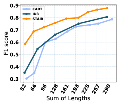
(a) Pendigits

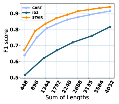
(b) Thursday-01-03

Figure 5. $F_{1}$ score with varying total rule lengths (Q2).

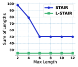
(a) PageBlock

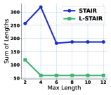
(b) Pendigits

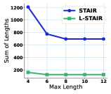
(c) Shuttle

(d) Pima

(e) Mammography

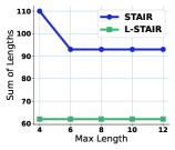
(f) Satimage-2

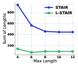
(g) Satellite

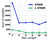
(h) SpamBase

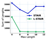
(i) Cover

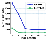
(j) Thursday-01-03

Figure 6. The effects of the maximal length $L_{m}$ on the total rule length (Q3).

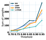
(a) PageBlock

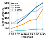
(b) Pendigits

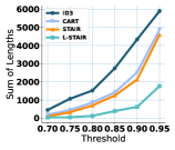
(c) Shuttle

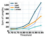
(d) Pima

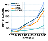
(e) Mammography

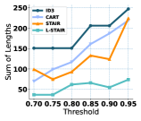
(f) Satimage-2

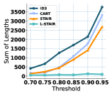
(g) Satellite

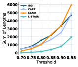
(h) SpamBase

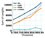
(i) cover

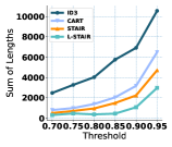
(j) Thursday-01-03

Figure 7. The effect of the threshold $F1_{m}$ on all methods (Q3).

In this set of experiments, we measure the total length of the rules produced by each algorithm when they produce trees with similar $F_{1}$ score. We set the maximal length of the rules $L_{m}$ to 10 and the $F_{1}$ score threshold $F1_{m}$ to 0.8. Because ID3 and CART do not use the $F_{1}$ score threshold in their algorithms, we tune their hyper-parameters to produce the simplest tree with a $F_{1}$ score slightly higher than 0.8. This ensures that all algorithms have the similar $F_{1}$ score. L-STAIR automatically determines the number of data partitions with initial partition number picked from {2, 4, 8}. We set the maximal iteration to $10$.

From the results shown in Table 2, we draw the following conclusions: (1) Compared to ID3 and CART, STAIR is able to produce much simpler rules which are amenable for humans to evaluate, significantly reducing the total length of the rules by up to 76.3% as shown in the results of the dataset Thursday-01-03. This is because the summarization and interpretation-aware optimization objective (Eq. 7) of STAIR simultaneously minimizes the complexity of the tree and maximizes the classification accuracy; (2) The performance of STAIR on the SpamBase dataset is not satisfying potentially due to its large dimensionality. SpamBase has 57 attributes. It thus might be over-complicated to use a single small tree to summarize the whole dataset; (3) L-STAIR which partitions the data and produces one tree for each data partition solves the problem mentioned in (2) and outperforms the basic STAIR by up to 91.37% as shown in the results of the dataset Cover.

Table 3. The number of partitions $n$ in L-STAIR (Q4).

	L-STAIR ($n$=2)			L-STAIR ($n$=4)			L-STAIR ($n$=8)
Dataset	Length	# of R	# of C	Length	# of R	# of C	Length	# of R	# of C
PageBlock	31	26	9	25	20	8	67	31	8
Pendigits	60	20	2	86	37	4	68	39	8
Shuttle	125	52	9	309	112	10	357	108	9
Pima	10	6	2	17	12	4	27	20	8
Mammography	31	20	6	24	15	5	29	21	8
Satimage-2	62	27	4	38	19	4	49	31	8
Satellite	70	18	2	78	28	4	209	74	8
SpamBase	150	51	8	218	73	10	278	72	9
Cover	402	117	5	470	136	4	621	195	8
Thursday-01-03	477	183	11	479	182	11	440	169	11

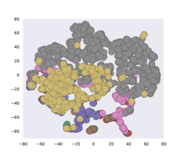
(a) PageBlock

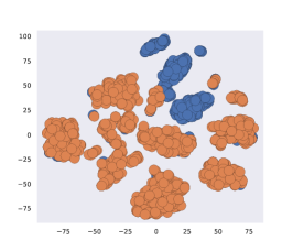
(b) Pendigits

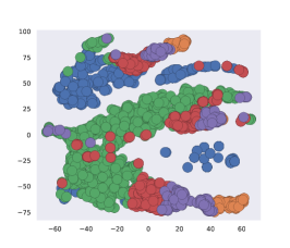
(c) Mammography

(d) Satimage-2

(e) SpamBase

(f) Satillite

Figure 8. Visualization of L-STAIR (Q5).

7.3. Comparison Against Baselines (Q2): $F_{1}$ Score

In this section, we evaluate the $F_{1}$ score of each algorithm when they produce a rule set with similar total length. For each dataset, we vary the total rule length by selecting 10 numbers within a range from 0 to the total rule length result with respect to the ID3 algorithm in Table 2. For instance, in Table 2 the total rule length of ID3 on the dataset Pendigits is 290. We thus select ten numbers: 29, 58, $\cdots$, 290 as the candidate total lengths.

Then given one total length $l$, we run ID3, CART, and STAIR in the following way to obtain the corresponding $F_{1}$ score: (1) For ID3, we gradually increase the depth of the tree until it generates a rule set with a total length slightly higher than $l$; (2) For CART, we first build a decision tree that is as accurate as possible and then prune it until it has a length close to $l$; (3) For STAIR, we update the breaking condition of Algorithm 1 such that it will terminate after reaching the length $l$. We run this experiment on the Pendigits and Thursday-01-03 datasets. As shown in Figure 5, STAIR is more accurate than ID3 and CART when they produce a rule set with the similar total length, indicating that given the same budget on the total rule length, STAIR produces rules with higher accuracy.

7.4. Effect of Hyper-parameters $L_{m}$ and $F1_{m}$ (Q3)

In this set of experiments, we first study how the maximal length $L_{m}$ affects STAIR and L-STAIR. We fix the F1 score threshold $F1_{m}$ as 80% and then vary $L_{m}$ from 2 to 12 and measure the how the total rule length changes. Note in some cases when $L_{m}$ is too small, e.g. 2, the learned tree cannot meet the F1 score requirement. As shown in Figure 6, as $L_{m}$ gets larger, the total rule length will get smaller. This is because with a looser constraint, STAIR gets a larger search space and hence better chance to find a simple tree. When STAIR gets better, L-STAIR will also gets better. Besides, we observe that L-STAIR could reach the minimal total rule length with smaller $L_{m}$. This shows the power and benefits of localization.

Next, we investigate how the F1 score threshold $F1_{m}$ affects STAIR and L-STAIR. We fix $L_{m}$ to 10 and vary $F1_{m}$ from 0.70 to 0.95. As shown in Figure 7, in most of the cases STAIR outperforms ID3 and CART, while L-STAIR consistently outperforms all other methods in all scenarios by up to 94.0% as shown in the results on the Cover dataset when the threshold is set as 0.95. The larger the $F1_{m}$ threshold is, the more L-STAIR outperforms other baselines. This is because partitioning allows L-STAIR to get a set of localized trees, each of which produces high accurate classification results on the corresponding data subset.

(a) PageBlock

(b) Pendigits

(c) Shuttle

(d) Pima

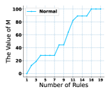
(e) Mammography

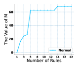
(f) Satimage-2

(g) Satellite

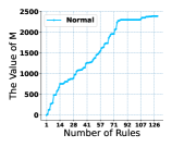
(h) SpamBase

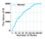
(i) Cover

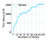
(j) Thursday-01-03

Figure 9. The dynamic $M$ during training (Q6).

7.5. Number of partitions in L-STAIR (Q4)

We study how the initial number of the partitions $n$ affects L-STAIR. In this set of experiments, $n$ is selected from {2, 4, 8}. In addition to the total rule length, we also report the number of rules in the final ruleset. From the results shown in Table 3, we have the following observations: (1) Compared to the results in Table 2, no matter what $n$ L-STAIR starts with, it consistently outperforms other methods; (2) L-STAIR always performs well when starting with a small $n$ compared to other initial $n$ values, indicating that $n$ is not a hyper-parameter that requires careful tuning.

Table 4. Multi-class classification: total rule length.

Dataset	ID3	CART	STAIR	L-STAIR
Wine Quality	5133	3217	2251	1538

Table 5. Multi-class classification: the number of partitions $n$ in L-STAIR

	L-STAIR ($n$=2)			L-STAIR ($n$=4)			L-STAIR ($n$=8)
Dataset	Length	# of R	# of C	Length	# of R	# of C	Length	# of R	# of C
Wine Quality	1642	614	11	1692	620	13	1538	635	17

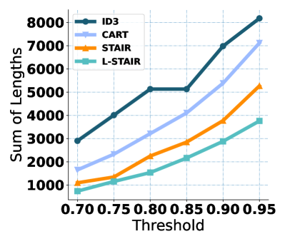
(a) Different Thresholds

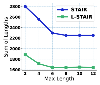
(b) Different $L_{m}$

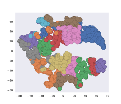
(c) Cluster Visualization

(d) Increasing of M

Figure 10. Multi-class dataset Wine Quality: ablation study

7.6. L-STAIR: Locality-Preserving (Q5)

Next, we evaluate if the partitioning of L-STAIR is able to preserve the locality of the data. We show this by visualizing its data partitioning. Before visualization, We apply T-SNE to embed the data into 2D. We plot different partitions in different colors. Due to space limit, we only plot the partitioning of 6 datasets. As shown in Figure 8, on all datasets the partitioning of L-STAIR preserves the locality. This thus guarantees the interpretability of each localized tree.

7.7. Dynamically Adjusting the Value of M (Q6)

In this set of experiment we show how STAIR automatically adjusts the value of stabilizer $M$ introduced in our summarization and interpretation-aware optimization objective (Sec. 4.2). To better understand the influence of a dynamically adjusting $M$, we use the number of rules produced in the training process as the reference variable, corresponding to the x-axis. From Figure 9, we observe: (1) The value of $M$ continuously increases during the training process to split nodes and thus produce valid rules; (2) The values of $M$ are different across different datasets, indicating that it is hard to get an appropriate $M$ by manual tuning.

7.8. Multi-class classification Problems (Q7)

We use this set of experiments to show that STAIR and L-STAIR are generally applicable to the more complicated multi-class classification problems. We use one of the most popular classification datasets Wine Quality (Cortez et al., 2009), which contains 4898 instances and 12 attributes. We regard the attribute “score” as the target which corresponds to integers within the range from 0 to 10 and run a classification task on it. Our STAIR and L-STAIR could be easily extended to multi-class settings by replacing the F1 score with the classification accuracy.

As shown in Table 4, we report the total rule length, same to the outlier detection scenario. We observe from the results: (1) L-STAIR and STAIR significantly outperform ID3 and Cart by up to 70.0%; (2) As shown in Table-5, the initial number $n$ of the partitions make little difference to the resulted lengths, indicating L-STAIR is not sensitive to the hyper-parameter $n$; (3) As illustrated in Figure 10(a) and Figure 10(b), STAIR and L-STAIR always outperform the baselines no matter how the accuracy threshold and the maximal rule length threshold vary; (4) Figure 10(c) visualizes the partitions produced by L-STAIR. The locality of the data partitions is well-preserved; (5) As shown in Figure 10(d), the dynamic update of the value of stabilizer $M$ is important in splitting the nodes and producing valid rules, similar to the case of outlier detection.

8. Related Work

Outlier Summarization and Interpretation. To the best of our knowledge, the problem of summarizing and interpreting outlier detection results has not been studied. Focused on a special type of outliers, Scorpion (Wu and Madden, 2013) produces explanations for outliers in aggregation queries by looking at the provenance of each outlier. If removing some objects from the aggregation significantly reduces the abnormality of a given outlier, these objects will be considered as the cause of this outlier. Similar to Scorpion, Cape (Miao et al., 2019) targets explaining the outliers in aggregation queries. But rather than rely on provenance, Cape uses the objects that counterbalance the outliers as the explanation. More specifically, if including some additional data objects into the aggregation query could neutralize an outlier, these objects effectively explain the outlier. Both works do not tackle the problems of summarizing outliers. Macrobase (Bailis et al., 2017) explains outliers by correlating them to some external attributes such as location or occurring time using associate rule mining. These external attributes are not used to detect anomalies. In many applications, however, such external attributes do not exist. Further, Macrobase only explains the outliers detected by its default density-based outlier detector customized to streaming data and does not easily generalize to other outlier detection methods.

Interpretable AI. Some works (Dunn et al., 2021; Phillips et al., 2020) target on interpreting the machine learning models, or understanding the model better with extra information (He et al., 2022). Some works such as LIME (Ribeiro et al., 2016), Anchor (Ribeiro et al., 2018), LORE (Guidotti et al., 2018) produce an explanation with respect to each inference. LIME (Ribeiro et al., 2016) explains the predictions of a classifier by learning a linear model locally around the prediction with respect to a particular testing object. It then uses the attributes that are most important to the linear prediction as the explanation. Because LIME has to learn one linear model for each individual object, using it to explain a large number of prediction results tends to prohibitively expensive. Some other methods (Ribeiro et al., 2018; Guidotti et al., 2018; Shrikumar et al., 2017; Bach et al., 2015; Lundberg and Lee, 2017) explain classification results in the similar fashion. Taking the explanations w.r.t all testing objects as input, Pedreschi et al. proposed to select a subset of the explanations to constitute a global explanation (Pedreschi et al., 2018). However, this work is not scalable to big datasets because it requires constructing the explanations for all testing objects. In addition, some techniques, including gradient-based (Simonyan et al., 2014; Sundararajan et al., 2017) and attention based (Bahdanau et al., 2015) methods, focus on particular types of deep learning model, thus hard to be used in the outlier summarization scenario. Lakkaraju et al (Lakkaraju et al., 2016) proposed to build a prediction model that is more interpretable than deep learning models. Follow-up methods (Sushil et al., 2018; Paçaci et al., 2019; Ming et al., 2019) work on augmenting the data to produce models with better interpretability. Instead of inventing new prediction models, our work focuses on explaining and summarizing the results produced by any outlier detection method.

Outlier Detection. Due to the importance of outlier detection(Cao et al., 2023), many unsupervised outlier detection methods have been proposed including the density based method LOF (Breunig et al., 2000), the statistical-based Mahalanobis method (Aggarwal, 2017), the distance-based methods (Angiulli and Pizzuti, 2002; Knorr and Ng, 1999; Ramaswamy et al., 2000), and Isolation Forest (Liu et al., 2008). These methods do not utilize any human-labeled data.

As a crowd sourcing-based method, HOD (Chai et al., 2020) proposed to leverage human input to improve the performance of outlier detection in text data. It produces some questions which once answered by humans, could help verify the status of multiple outlier candidates returned by the unsupervised outlier detectors. However, the question-generation process of HOD is still time-consuming. In addition, instead of focusing on text data, our STAIR method is generally applicable to different types of data including numerical, categorical, and text data.

Decision Tree Algorithms. Because a simple tree tends to avoid overfitting and have better generalization ability, CART (Breiman et al., 1984) proposed to prune a learned decision tree to lift its performance in a post-processing step. It will remove a node in the tree if the cross-validation error rate does not increases. However, unlike our STAIR which treats producing simple hence human interpretable rules as the first class citizen in its objective, the post-processing of CART is not very effective in minimizing the complexity of the rules, as confirmed in our experiments. Other decision tree algorithms (Biggs et al., 1991; Kass, 1980; Ritschard, 2013) mostly suffer from the same problem that the simplicity of the rules is not considered to be as important as the classification accuracy.

9. Conclusion

This work targets reducing the human effort in evaluating outlier detection results. To achieve this goal, we propose STAIR to learn a compact set of human understandable rules which summarizes anomaly detection results into groups and explains why each group of objects is considered to be abnormal. It features an outlier summarization and interpretation-ware optimization objective, a learning algorithm which optimally maximizes this objective in each iteration, and a partitioning driven STAIR approach which simultaneously divides the data and produces localized rules for each data partition. Experiment results show that STAIR effectively summarize the outlier detection results with human interpretable rules, where the complexity of the rules is much lower than those produced by other decision tree methods.

References

- (1)
- Aggarwal (2017) Charu C. Aggarwal. 2017. Outlier Analysis: Second Edition. Springer.
- Angiulli and Pizzuti (2002) Fabrizio Angiulli and Clara Pizzuti. 2002. Fast Outlier Detection in High Dimensional Spaces. In PKDD. 15–26.
- Bach et al. (2015) Sebastian Bach, Alexander Binder, Grégoire Montavon, Frederick Klauschen, Klaus-Robert Müller, and Wojciech Samek. 2015. On pixel-wise explanations for non-linear classifier decisions by layer-wise relevance propagation. PloS one 10, 7 (2015), e0130140.
- Bahdanau et al. (2015) Dzmitry Bahdanau, Kyunghyun Cho, and Yoshua Bengio. 2015. Neural Machine Translation by Jointly Learning to Align and Translate. In ICLR.
- Bailis et al. (2017) Peter Bailis, Edward Gan, Samuel Madden, Deepak Narayanan, Kexin Rong, and Sahaana Suri. 2017. Macrobase: Prioritizing attention in fast data. In Proceedings of the 2017 ACM International Conference on Management of Data. ACM, 541–556.
- Batra and Agrawal (2018) Mridula Batra and Rashmi Agrawal. 2018. Comparative Analysis of Decision Tree Algorithms. In Nature Inspired Computing, Bijaya Ketan Panigrahi, M. N. Hoda, Vinod Sharma, and Shivendra Goel (Eds.). Springer Singapore, Singapore, 31–36.
- Biggs et al. (1991) David Biggs, Barry De Ville, and Ed Suen. 1991. A method of choosing multiway partitions for classification and decision trees. Journal of applied statistics 18, 1 (1991), 49–62.
- Breiman et al. (1984) L. Breiman, J. H. Friedman, R. A. Olshen, and C. J. Stone. 1984. Classification and Regression Trees. Wadsworth and Brooks, Monterey, CA.
- Breunig et al. (2000) Markus M. Breunig, Hans-Peter Kriegel, Raymond T. Ng, and Jörg Sander. 2000. LOF: Identifying Density-Based Local Outliers. In SIGMOD. 93–104.
- Cao et al. (2023) Lei Cao, Yizhou Yan, Yu Wang, Samuel Madden, and Elke A Rundensteiner. 2023. AutoOD: Automatic Outlier Detection. Proceedings of the ACM on Management of Data 1, 1 (2023), 1–27.
- Chai et al. (2020) Chengliang Chai, Lei Cao, Guoliang Li, Jian Li, Yuyu Luo, and Samuel Madden. 2020. Human-in-the-Loop Outlier Detection. In Proceedings of the 2020 ACM SIGMOD International Conference on Management of Data (Portland, OR, USA) (SIGMOD ’20). Association for Computing Machinery, New York, NY, USA, 19–33. https://doi.org/10.1145/3318464.3389772
- Cortez et al. (2009) Paulo Cortez, António Cerdeira, Fernando Almeida, Telmo Matos, and José Reis. 2009. Modeling wine preferences by data mining from physicochemical properties. Decis. Support Syst. 47, 4 (2009), 547–553.
- Dunn et al. (2021) Jack Dunn, Luca Mingardi, and Ying Daisy Zhuo. 2021. Comparing interpretability and explainability for feature selection. CoRR abs/2105.05328 (2021).
- Elaidi et al. (2018) Halima Elaidi, Zahra Benabbou, and Hassan Abbar. 2018. A comparative study of algorithms constructing decision trees: ID3 and C4.5. In Proceedings of the International Conference on Learning and Optimization Algorithms: Theory and Applications, LOPAL 2018, Rabat, Morocco, May 2-5, 2018. 26:1–26:5.
- Ester et al. (1996) Martin Ester, Hans-Peter Kriegel, Jörg Sander, and Xiaowei Xu. 1996. A density-based algorithm for discovering clusters in large spatial databases with noise.. In Kdd, Vol. 96. 226–231.
- Fu and Perry (2020) Wei Fu and Patrick O Perry. 2020. Estimating the number of clusters using cross-validation. Journal of Computational and Graphical Statistics 29, 1 (2020), 162–173.
- Guidotti et al. (2018) Riccardo Guidotti, Anna Monreale, Salvatore Ruggieri, Dino Pedreschi, Franco Turini, and Fosca Giannotti. 2018. Local Rule-Based Explanations of Black Box Decision Systems. CoRR abs/1805.10820 (2018).
- He et al. (2022) Zexue He, Yu Wang, Julian J. McAuley, and Bodhisattwa Prasad Majumder. 2022. Controlling Bias Exposure for Fair Interpretable Predictions. In EMNLP (Findings). Association for Computational Linguistics, 5854–5866.
- Kanungo et al. (2002) T. Kanungo, D.M. Mount, N.S. Netanyahu, C.D. Piatko, R. Silverman, and A.Y. Wu. 2002. An efficient k-means clustering algorithm: analysis and implementation. IEEE Transactions on Pattern Analysis and Machine Intelligence 24, 7 (2002), 881–892.
- Kass (1980) Gordon V Kass. 1980. An exploratory technique for investigating large quantities of categorical data. Journal of the Royal Statistical Society: Series C (Applied Statistics) 29, 2 (1980), 119–127.
- Knorr and Ng (1999) Edwin M. Knorr and Raymond T. Ng. 1999. Finding Intensional Knowledge of Distance-Based Outliers. In In VLDB. 211–222.
- Lakkaraju et al. (2016) Himabindu Lakkaraju, Stephen H. Bach, and Jure Leskovec. 2016. Interpretable Decision Sets: A Joint Framework for Description and Prediction. In KDD. ACM, 1675–1684.
- Liu et al. (2008) Fei Tony Liu, Kai Ming Ting, and Zhi-Hua Zhou. 2008. Isolation forest. In 2008 Eighth IEEE International Conference on Data Mining. IEEE, 413–422.
- Lundberg and Lee (2017) Scott M Lundberg and Su-In Lee. 2017. A unified approach to interpreting model predictions. Advances in neural information processing systems 30 (2017).
- Miao et al. (2019) Zhengjie Miao, Qitian Zeng, Chenjie Li, Boris Glavic, Oliver Kennedy, and Sudeepa Roy. 2019. CAPE: Explaining Outliers by Counterbalancing. Proc. VLDB Endow. 12, 12 (2019), 1806–1809.
- Ming et al. (2019) Yao Ming, Huamin Qu, and Enrico Bertini. 2019. RuleMatrix: Visualizing and Understanding Classifiers with Rules. IEEE Trans. Vis. Comput. Graph. 25, 1 (2019), 342–352.
- Paçaci et al. (2019) Görkem Paçaci, David Johnson, Steve McKeever, and Andreas Hamfelt. 2019. ”Why Did You Do That?” - Explaining Black Box Models with Inductive Synthesis. In ICCS (5) (Lecture Notes in Computer Science, Vol. 11540). Springer, 334–345.
- Pedreschi et al. (2018) Dino Pedreschi, Fosca Giannotti, Riccardo Guidotti, Anna Monreale, Luca Pappalardo, Salvatore Ruggieri, and Franco Turini. 2018. Open the Black Box Data-Driven Explanation of Black Box Decision Systems. CoRR abs/1806.09936 (2018).
- Phillips et al. (2020) P Jonathon Phillips, Carina A Hahn, Peter C Fontana, David A Broniatowski, and Mark A Przybocki. 2020. Four principles of explainable artificial intelligence. Gaithersburg, Maryland (2020).
- Quinlan (1986) J. Ross Quinlan. 1986. Induction of Decision Trees. Mach. Learn. 1, 1 (1986), 81–106.
- Quinlan (1993) J. Ross Quinlan. 1993. C4.5: Programs for Machine Learning. Morgan Kaufmann.
- Ramaswamy et al. (2000) Sridhar Ramaswamy, Rajeev Rastogi, and Kyuseok Shim. 2000. Efficient algorithms for mining outliers from large data sets. In ACM SIGMOD Record, Vol. 29. ACM, 427–438.
- Ribeiro et al. (2016) Marco Túlio Ribeiro, Sameer Singh, and Carlos Guestrin. 2016. ”Why Should I Trust You?”: Explaining the Predictions of Any Classifier. In KDD. ACM, 1135–1144.
- Ribeiro et al. (2018) Marco Túlio Ribeiro, Sameer Singh, and Carlos Guestrin. 2018. Anchors: High-Precision Model-Agnostic Explanations. In AAAI. AAAI Press, 1527–1535.
- Ritschard (2013) Gilbert Ritschard. 2013. CHAID and earlier supervised tree methods. In Contemporary issues in exploratory data mining in the behavioral sciences. Routledge, 70–96.
- Safavian and Landgrebe (1991) S.R. Safavian and D. Landgrebe. 1991. A survey of decision tree classifier methodology. IEEE Transactions on Systems, Man, and Cybernetics 21, 3 (1991), 660–674. https://doi.org/10.1109/21.97458
- Shrikumar et al. (2017) Avanti Shrikumar, Peyton Greenside, and Anshul Kundaje. 2017. Learning Important Features Through Propagating Activation Differences. In ICML (Proceedings of Machine Learning Research, Vol. 70). PMLR, 3145–3153.
- Simonyan et al. (2014) Karen Simonyan, Andrea Vedaldi, and Andrew Zisserman. 2014. Deep Inside Convolutional Networks: Visualising Image Classification Models and Saliency Maps. In ICLR (Workshop Poster).
- Sundararajan et al. (2017) Mukund Sundararajan, Ankur Taly, and Qiqi Yan. 2017. Axiomatic Attribution for Deep Networks. In ICML (Proceedings of Machine Learning Research, Vol. 70). PMLR, 3319–3328.
- Sushil et al. (2018) Madhumita Sushil, Simon Suster, and Walter Daelemans. 2018. Rule induction for global explanation of trained models. In BlackboxNLP@EMNLP. Association for Computational Linguistics, 82–97.
- Wu and Madden (2013) Eugene Wu and Samuel Madden. 2013. Scorpion: Explaining Away Outliers in Aggregate Queries. Proc. VLDB Endow. 6, 8 (2013), 553–564.