The Bounds of Mediated Communication

Abstract

We study the bounds of mediated communication in sender-receiver games in which the sender’s payoff is state-independent. We show that the feasible distributions over the receiver’s beliefs under mediation are those that induce zero correlation, but not necessarily independence, between the sender’s payoff and the receiver’s belief. Mediation attains the upper bound on the sender’s value, i.e., the Bayesian persuasion value, if and only if this value is attainable under unmediated communication, i.e., cheap talk. The lower bound is given by the cheap talk payoff. We provide a geometric characterization of when mediation strictly improves on this using the quasiconcave and quasiconvex envelopes of the sender’s value function. In canonical environments, mediation is strictly valuable when the sender has countervailing incentives in the space of the receiver’s belief. We apply our results to asymmetric-information settings such as bilateral trade and lobbying and explicitly construct mediation policies that increase the surplus of the informed and uninformed parties with respect to unmediated communication.

1 Introduction

Consider a receiver who faces a decision problem under uncertainty about some payoff-relevant finite state. The state is privately observed by a sender who can communicate with the receiver to influence her decision and has a final payoff that depends on the receiver’s action only, that is, the sender has transparent motives. These situations are pervasive in economics: a seller has superior information about the quality of a good and always wants to maximize the probability of selling it to buyers.

In these settings, one of two extreme assumptions is usually considered: 1) The sender can commit ex-ante to any information policy, such as an experiment that conveys verifiable information to the receiver, or 2) The sender cannot commit to any experiment, their private information is not verifiable (i.e., it is soft), but they can freely send messages to the receiver. The first case has been extensively analyzed in recent years and corresponds to the Bayesian persuasion model of Kamenica and Gentzkow (2011). The second case corresponds to a game of strategic information transmission or cheap talk as introduced in Crawford and Sobel (1982). It is well known that with commitment, the sender can often achieve a strictly higher payoff than the one obtained by conveying no information. Perhaps more surprisingly, Chakraborty and Harbaugh (2010) and Lipnowski and Ravid (2020) showed that the sender can also achieve a strictly higher payoff under cheap talk than without communication, that is communication is also often strictly valuable.

In this paper, we revisit and adapt the intermediate case of mediated communication introduced in Myerson (1982). We enlarge the set of players by considering a third-party mediator. The mediator cannot take the relevant decision in place of the receiver and is uninformed about the state, hence they must resort to information willingly shared by the sender. However, the mediator can commit to any communication mechanism that collects reports from the sender and sends messages to the receiver. In the buyer-seller example above, the mediator can represent an advertising agency or a rating agency with a prominent reputation that collects reports from the seller and conveys credible information to the buyers.

We focus on the case where the mediator’s preference is aligned with the sender, hence they act to maximize the sender’s payoff. Clearly, the sender-optimal values across the three protocols considered are weakly ordered because the space of feasible information policies becomes smaller from persuasion to mediation and from mediation to cheap talk: $BP\geq MD\geq CT$. With this, we decompose the gap between Bayesian persuasion and cheap talk as follows:

$$\underset{\text{Value of Commitment}}{\underbrace{BP-CT}}=\underset{\text{Value of Elicitation}}{\underbrace{BP-MD}}+\underset{\text{Value of Mediation}}{\underbrace{MD-CT}.}$$

The gap $BP-CT$ represents the value of commitment for the sender. The first component of this gap is $BP-MD$ which captures the value of elicitation. In both persuasion and mediation, there is an entity with commitment power, the sender and the mediator, respectively. However, the mediator is not directly informed about the state and has to elicit this information in an incentive-compatible way. Differently, the gap $MD-CT$ captures the value of mediation because it corresponds to the additional value that an uninformed third party with commitment can secure to the sender when the latter has no commitment power. Our results provide sufficient and necessary conditions such that the values of elicitation and mediation are strictly positive.

Outline of the results

By the revelation principle, the mediator acts “as-if” selecting a communication equilibrium outcome of the sender-receiver game. However, differently from Myerson (1982), we adopt a belief-based approach to mediation that connects us more directly to Bayesian persuasion and cheap talk. We show that the feasible distributions of receiver’s beliefs are those that induce zero correlation, but not necessarily independence, between the sender’s payoff and the receiver’s belief. This condition translates the truth-telling constraint of the sender from the space of mechanisms to the space of beliefs. We can then represent the optimal mediation problem as a linear program under moment constraints in the belief space: the standard Bayes plausibility constraint and the zero-correlation constraint.

Exploiting this rewriting of the mediation problem, we show that the sender can attain the optimal persuasion payoff under mediation if and only if this value can be attained under cheap talk. Therefore, we show that when elicitation is valueless, so is mediation. Given that the value of commitment is often strictly positive, this implies that an uninformed mediator cannot usually guarantee the same value that the sender would achieve with commitment.

Next, we introduce two novel key concepts for cheap talk: the cheap talk hull is the affine hull of all the supports of cheap-talk optimal distributions of the receiver’s beliefs, and the full-dimensionality condition holds when the cheap talk hull covers the entire space of the receiver’s beliefs. This condition is satisfied for almost every prior when the receiver’s action set is finite and, at every binary prior such that the babbling equilibrium is not sender optimal. Moreover, we show that full dimensionality is satisfied at a given prior when the value of cheap talk is constant around that prior.

Under the full-dimensionality condition, we characterize the cases where elicitation and mediation are strictly valuable, that is, $BP>MD$ and $MD>CT$, respectively. Elicitation is strictly valuable if and only if there exists a belief $\mu\in\Delta(\Omega)$ of the receiver such that the maximum cheap talk value at $\mu$ is strictly higher than the maximum cheap talk value at the prior $p$. Mediation is strictly valuable if and only if there exist two beliefs $\mu_{+},\mu_{-}\in\Delta(\Omega)$ of the receiver that are colinear with the prior $p$ and such that the maximum cheap talk value at $p$ lies strictly between the maximum cheap talk value at $\mu_{+}$ and the minimum cheap talk value at $\mu_{-}$. In particular, we construct an improving mediation plan by randomizing over distributions of beliefs that include cheap talk equilibria at $\mu_{+}$ and $\mu_{-}$ respectively. This randomization is not a valid cheap talk equilibrium at $p$, yet it satisfies all the incentive compatibility requirements of communication equilibria, hence it is feasible under mediation. We prove these results by first providing distinct sufficient and necessary conditions for the values of elicitation and mediation to be strictly positive without any additional assumption and then show that under full dimensionality these conditions are the same. All the aforementioned conditions admit geometric characterizations in terms of the quasiconcave and quasiconvex envelopes of the sender’s value function.

In several canonical settings, we find that meditation has a strictly positive value when the sender has countervailing incentives in the space of the receiver’s beliefs, that is, when the sender would like to induce more optimistic beliefs for some realized messages and more pessimistic beliefs for some others. In binary-state settings or when the sender’s utility depends on the receiver’s conditional expectation only, this translates to the failure of a weak form of single-crossing. For multidimensional environments with strictly quasiconvex utility for the sender, countervailing incentives are captured by the non-monotonicity of the restriction of the sender’s utility to the edges of the simplex.

We illustrate how our constructive approach is useful in applications to find mediation plans that improve the sender’s expected payoff. We revisit the think tank example in Lipnowski and Ravid (2020) by assuming that the think tank acts as a mediator between an interest group (the sender) and the lawmaker (the receiver). In this case, countervailing incentives arise because the interest group strictly prefers the lawmaker to approve one of several new policies as opposed to retaining the status quo. Similarly, we apply our results to study advertising or rating agencies that operate as mediators between sellers and buyers. In this case, countervailing incentives can arise because of reputation concerns of the seller or because of non-monotone preferences over risky prospects (e.g., mean-variance) of the receiver. For these examples, both elicitation and mediation are usually strictly valuable, thereby rationalizing the ubiquitous presence of intermediaries in these markets. In addition, we often find that the extra randomness introduced by the mediator strictly benefits the receiver as well, that is, in these cases mediation is (ex-ante) strictly Pareto superior to unmediated communication.

Finally, we discuss some additional implications of our results as well as some extensions. For long cheap talk (see Aumann and Hart (2003)) and repeated games with asymmetric information (see Hart (1985)), our results characterize the environments where the sender’s payoff under the best correlated equilibrium is strictly higher than the one obtained when we restrict to Nash equilibria.

1.1 Illustrative Example

We illustrate the geometric comparison of Bayesian persuasion, mediation, and cheap talk by a simple advertising model that compares the case where a seller directly communicates with a buyer to the case where the seller hires an advertising agency to mediate communication.

Consider a seller planning to commercialize a new product. The product’s quality $\omega\in\Omega=\{0,1\}$ is privately known by the seller, and a buyer has a prior $p\in(0,0.55)$ on the quality being good ($\omega=1$). We first consider the case when the seller can only communicate by cheap talk messages. After observing the message, the buyer updates her belief about the quality to $\mu\in[0,1]$ and decides whether to purchase the good or take her outside option with quality $\varepsilon\in[0,1]$. Each buyer is privately informed about the outside option, but the seller knows only that the distribution of $\varepsilon$ is $G$. In particular, we assume that $G$ has a unimodal density $g$, that is, $G$ is strictly convex up to some point $\hat{\varepsilon}$ and concave beyond that point.

The market is competitive, and we normalize the price of the good and the outside option to $1$. Thus, when the buyers’ posterior belief is $\mu$, the buyers purchasing the good are those such that $\varepsilon\leq\mu$, for a total mass of $G(\mu)$. The seller’s overall utility depends on the total demand for the good and on a component of reputation concern of the seller, that is, the seller’s indirect utility $\tilde{V}(\mu,\omega)$ given posterior $\mu$ and quality $\omega$ is

$$\tilde{V}(\mu,\omega)=(1-\delta)G(\mu)+\delta(\omega-\mu).$$

The linear term $\delta(\omega-\mu)$ captures the reputation effect, where $\delta>0$ measures the positive effect of a surprisingly good product on the seller’s future payoff. Conversely, when $\omega<\mu$, there is a negative reputation effect due to an unexpectedly bad product. As the state $\omega$ is privately known and the seller’s payoff function is additively separable in $\tilde{V}(\mu,\omega)$, the seller acts to maximize

$$V(\mu)=(1-\delta)G(\mu)-\delta\mu.$$

Therefore, in what follows we consider $V$ to be the payoff function of the seller. Under our assumptions on $G$, this indirect utility $V$ is a rotated S-shaped function as illustrated in Figure 1. In this case, an intermediate level of reputation concern induces countervailing incentives for the sender. For example, in Figure 1, for posteriors $\mu$ just before $3/4$, the sender would like the buyer to be more optimistic about the product quality, whereas, for posteriors above $3/4$, the seller would like the buyer to be more pessimistic.

From Lipnowski and Ravid (2020), we know that the seller-optimal cheap talk value at any prior is given by the quasiconcave envelope of $V$ at that prior, which is the dotted red line in Figure 1. In particular, the best cheap talk equilibrium for the seller at $p$ is such that posterior $\mu=0.55$ is induced with probability $p/0.55$ and $\mu=0$ is induced with probability $1-p/0.55$. Hence, the seller’s optimal payoff under cheap talk is $0$.

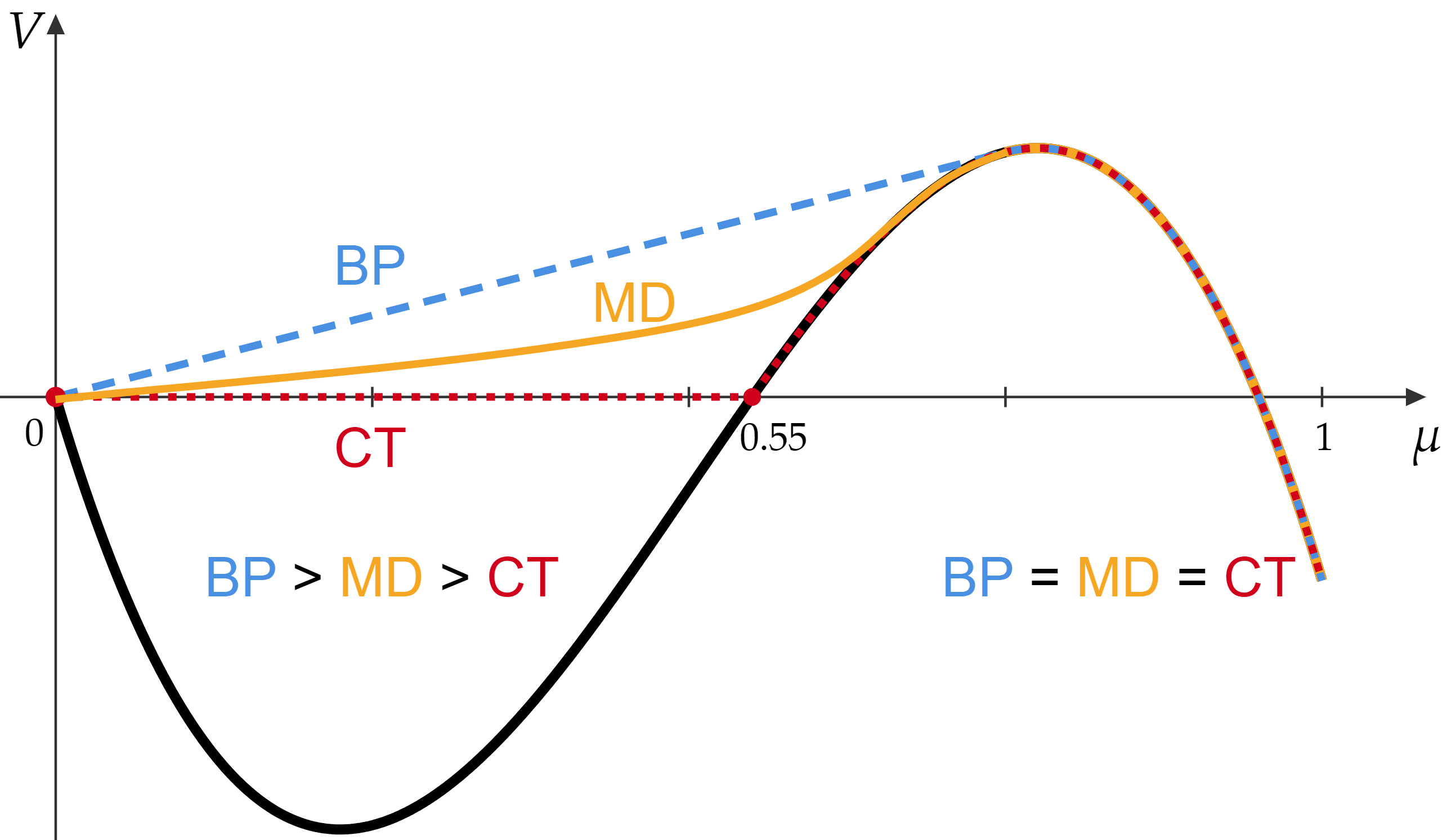
Figure 1: Comparison of Bayesian persuasion, mediation, and cheap talk

The colored lines represent the seller’s optimal payoff from Bayesian persuasion (blue dashed), mediation (yellow solid), and cheap talk (red dashed). The discussion here focuses on the case $p\in(0,0.55)$, where the three lines do not coincide.

Next, we show that the seller can obtain a strictly higher payoff by hiring an advertiser (the mediator) who can credibly commit to revealing information about the quality of the good to the buyer. The advertiser does not have the expertise to assess the exact quality of the good and can only convey information the seller reports. To maintain credibility, the advertiser designs the information structure so that the seller is willing to report truthfully. The contract between the seller and the advertiser is fixed and binds the seller to pay the advertiser a fixed fraction of its revenue, and the advertiser maximizes the seller’s expected payoff. In this case, the advertiser can strictly increase the seller’s expected payoff by introducing randomness to the message distribution conditional on the seller’s quality report. For instance, this randomness conditional on the seller’s quality reports can be interpreted as the use of inessential visual effects or vague language in the advertising campaign for the product.

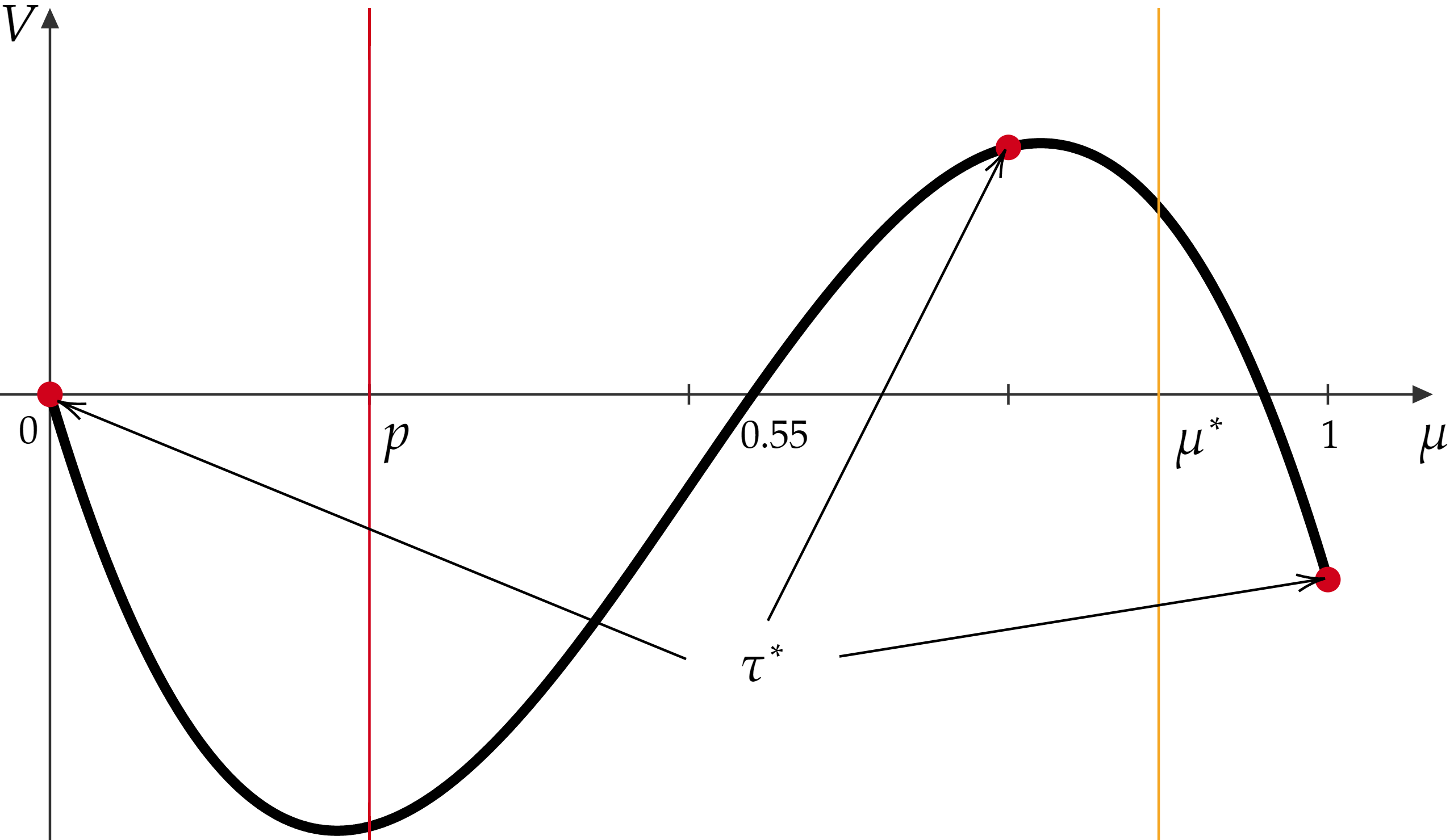
Figure 2: Construction of strictly improving mediation plan

Now, we construct a distribution of beliefs that is feasible for the advertiser and that yields a strict improvement for the seller with respect to direct communication. First fix $\xi\in(0,1)$ such that $\xi\cdot V(3/4)\cdot(3/4-p)+(1-\xi)\cdot V(1)\cdot(1-p)=0$. With this, fix the belief $\mu^{*}=\xi\cdot 3/4+(1-\xi)\cdot 1$, highlighted by the yellow line in Figure 2, and observe that there exists $\alpha>1$ such that $\alpha p+(1-\alpha)\mu^{*}=0$. Now, consider the distribution of buyers’ beliefs supported on $\left\{0,3/4,1\right\}$ given by

$$\tau^{*}=\left\{(0;1/\alpha),(3/4;(\alpha-1)\xi/\alpha),(1;(\alpha-1)(1-\xi)/\alpha)\right\}.$$

The three points in the support of this distribution are highlighted by the red dots in Figure 2. Note that this distribution does not correspond to a cheap talk equilibrium, as the seller would always have the incentive to induce $\mu=3/4$ at every state.

By construction, $\tau^{*}$ averages to $p$ and induces zero correlation between the buyers’ beliefs $\mu$ and the seller’s payoff $V(\mu)$. In Theorem 1 below, we show that this is necessary and sufficient for $\tau^{*}$ to be implementable under mediation. Finally, one can verify that the seller’s expected payoff under this distribution of beliefs is

$$\tfrac{\alpha-1}{\alpha}(\xi\cdot V(3/4)+(1-\xi)\cdot V(1))>0$$

yielding a strict improvement. This payoff is not the best payoff the mediator can secure for the sender, but shows that the value of mediation is strictly positive. With a small enough commission rate, the seller strictly benefits from hiring an advertiser to mediate communication.

If the mediator has the expertise to assess the quality of the goods without relying on the seller’s reports, they design (and commit to) a test/information structure about the quality of the goods that is revealed to the buyer. The seller has a strict incentive to take this option because it relaxes the truth-telling constraint and allows the seller to induce any Bayesian persuasion outcome. For instance, the mediator can commit to sending messages $\mu=3/4$ with probability $4p/3$ and $\mu=0$ with probability $1-4p/3$. This information structure induces the optimal Bayesian persuasion outcome (one may verify this by concavification), and the optimal persuasion payoff is greater than the payoff of the mediation plan we illustrated. Indeed, since the value of commitment is strictly positive, our Theorem 2 implies that the value of elicitation is strictly positive as well. Figure 1 plots the CT value (red), the MD value (yellow), and the BP value (blue) over all the priors. Both elicitation and mediation are strictly valuable at every $p\in(0,0.55)$.

Finally, the buyer is strictly better off under the mediation plan we constructed than under the sender-optimal cheap talk equilibrium or the Bayesian persuasion outcome. Note that the buyer’s indirect utility $V_{R}(\mu)=\mu G(\mu)+\int_{\mu}^{1}\varepsilon\mathop{}\!\mathrm{d}G(\varepsilon)$ is strictly convex, and the induced distributions of posteriors are supported on $\{0,3/4,1\}$ under mediation and $\{0,3/4\}$ under persuasion. Hence, the distribution of beliefs under mediation is a mean-preserving spread of that under persuasion, which leads to a strictly higher buyer payoff. Direct calculation shows that the buyer’s payoff under the proposed mediation plan is also strictly higher than under cheap talk.

1.2 Literature review

Our work uses the “belief-based approach,” a widely adopted methodology in the study of sender-receiver games. Kamenica and Gentzkow (2011) characterizes the sender’s optimal payoff under persuasion as the concave envelope of the sender’s value function, and Lipnowski and Ravid (2020) shows that the sender’s best payoff under cheap talk with transparent motives is characterized by the quasiconcave envelope of her value function.

Our work also belongs to the literature on mediated communication initiated by Myerson (1982) and Forges (1986). Recent works on this topic study the comparison between mediation and other specific forms of communication in the uniform-quadratic case of Crawford and Sobel (1982). Blume et al. (2007) focuses on contrasting noisy cheap talk with cheap talk, while Goltsman et al. (2009) compares mediation, (long) cheap talk, and delegation. Differently, we completely characterize the comparison between persuasion, mediation, and cheap talk under state-independent preferences for the sender, but without additional parametric assumptions.

The most related paper in the mediation literature is Salamanca (2021), where mediated communication for finite games is analyzed using a recommendation approach similar to the original one in Myerson (1982). Our analysis differs from the one in Salamanca (2021) for several reasons. First, the two models are not nested since we focus on the transparent-motive case but we allow for arbitrary action space for the receiver. Second, our analysis is entirely carried out with a belief-based approach as opposed to the recommendation approach they use. Our approach not only allows us to readily derive the same “virtual-utility” representation of the sender-optimal value of mediation but also to compare more directly mediated communication with persuasion and cheap talk. In fact, the main differences between the two analyses are on the result side. While Salamanca (2021) focuses on deriving strong duality for the recommendation-based mediation problem, we use a more direct perturbation approach that allows us to completely characterize when elicitation and mediation are valuable for finite games at almost all prior beliefs. Moreover, we provide several sufficient conditions such that our characterization extends to infinite-action games.

Some works in the mediation literature allow for transfers between the informed party and the intermediary. For example, Corrao (2023) considers an optimal mediation problem with transfers where the mediator maximizes their revenue from payments from the informed party. Importantly, he considers a state-dependent payoff for the sender and imposes a strict single-crossing condition. This considerably expands the set of implementable outcomes. In fact, Corrao (2023) shows that in a binary-state setting, every distribution of the receiver’s beliefs is implementable. This is in sharp contrast with the zero-correlation restriction imposed by the truthtelling constraint in our setting with transparent motives and where transfers are not allowed.

Finally, our work is related to recent papers studying Bayesian persuasion with limited commitment or additional constraints (Lin and Liu, 2023; Lipnowski et al., 2022; Koessler and Skreta, 2023; Doval and Skreta, 2023). Like mediation, the communication protocols studied in these works can be seen as intermediate cases between Bayesian persuasion and (single-round) cheap talk. The transparent-motive assumption sometimes makes these intermediate cases attain one of the two bounds given by persuasion and cheap talk. For example, the credible information structures in Lin and Liu (2023) are the same ones that are feasible under persuasion, when the sender has transparent motives. Under the same assumption, Lipnowski and Ravid (2020) show that the sender’s optimal payoff in the long cheap talk model of Aumann and Hart (2003) is the same as the one of single-round cheap talk. Differently, in this paper, we show that the optimal sender’s value under mediation can be strictly between the two bounds and we completely characterize when this is the case in several settings.

Outline of the paper

Section 2 introduces the model. Section 3 characterizes the feasible distributions of the receiver’s beliefs under mediation. Section 4 presents our main comparison results for the simple case of binary states. This allows us to describe the basic intuition of our results without the technical challenges of the general case. Sections 5 and 6 present our general results on the comparison of mediation, Bayesian persuasion, and cheap talk. Section 7 applies our results to the case where the sender’s utility is strictly quasiconvex. Section 8 discusses some extensions and future research. All the proofs are relegated to Appendix A.

2 The Model

Our model consists of three players: a sender, a receiver, and a mediator. Let $\Omega$ be a finite state space with $|\Omega|=n$. The state $\omega\in\Omega$ is drawn according to a full-support common prior $p\in\Delta(\Omega)$, and the realization of $\omega$ is the sender’s private information. The receiver does not know the realized $\omega$ and takes a payoff-relevant action $a\in A$, where $A$ is a compact metric space. We assume the sender has a state-independent utility function $u_{S}:A\to\mathbb{R}$, and the receiver has utility $u_{R}:\Omega\times A\to\mathbb{R}$. Both utility functions are continuous.

The sender and receiver communicate through the mediator, who commits to a communication mechanism $\sigma:R\to\Delta(M)$ without knowing $\omega$, where $R$ is the reporting space for the sender and $M$ is the space of messages for the receiver. After observing $\omega$, the sender sends a report $r\in R$ to the mediator. Given the report, the mediator draws a random message $m\in M$ according to $\sigma$ and sends it to the receiver, who then takes an action $a\in A$. We consider the communication game $\Gamma_{\sigma}$ induced by $\sigma$ and focus on the Bayes-Nash equilibria of $\Gamma_{\sigma}$, also known as the communication equilibria (see Myerson (1982) and Forges (1986)). We assume that the mediator is perfectly aligned with the sender and selects a mechanism and an equilibrium to maximize the sender’s expected utility.

Any mechanism $\sigma$ and a communication equilibrium in $\Gamma_{\sigma}$ induce an outcome distribution $\pi\in\Delta(\Omega\times A)$. Applying the Revelation Principle (Myerson, 1982; Forges, 1986), it is without loss to consider outcome distributions induced by direct incentive-compatible mechanisms, that is, a communication equilibrium where the mediator asks the sender for a state report in $R=\Omega$, provides an action recommendation in $M=A$ to the receiver, and the sender truthfully reports the state while the receiver follows the action recommendation.

Fact.

Any outcome distribution $\pi\in\Delta(\Omega\times A)$ is induced by some communication equilibrium if and only if it satisfies:

• Consistency: $\operatorname{marg}_{\Omega}{\pi}=p$

• Obedience: For all $a,a^{\prime}\in A$, $\mathbb{E}_{\pi^{a}}[u_{R}(\omega,a)]\geq\mathbb{E}_{\pi^{a}}[u_{R}(\omega,a^{\prime})]$, where $\pi^{a}\in\Delta(\Omega)$ is a version of the conditional probability given $a\in A$;

• Honesty: For all $\omega,\omega^{\prime}\in\Omega$, $\mathbb{E}_{\pi^{\omega}}[u_{S}(a)]\geq\mathbb{E}_{\pi^{\omega^{\prime}}}[u_{S}(a)]$, where $\pi^{\omega}\in\Delta(A)$ is the conditional probability given $\omega\in\Omega$.

We say that $\pi\in\Delta(\Omega\times A)$ is a communication equilibrium (CE) outcome if it satisfies (i), (ii), and (iii).

3 Belief-based Approach to Mediated Communication

Instead of focusing on CE outcomes, we consider distributions over the receiver’s posteriors $\tau\in\Delta(\Delta(\Omega))$ and the sender’s indirect utility $V:\Delta(\Omega)\to\mathbb{R}$ in terms of the receiver’s posterior. Define the indirect value correspondence $\mathbf{V}:\Delta(\Omega)\rightrightarrows\mathbb{R}$ by

$$\mathbf{V}(\mu):=\operatorname*{co}\left(u_{S}\left(\operatorname*{argmax}_{a\in A}\mathbb{E}_{\mu}[u_{R}(\omega,a)]\right)\right).$$

For every posterior $\mu\in\Delta(\Omega)$, the set $\mathbf{V}(\mu)$ collects all the possible (expected) sender’s payoffs that can be attained by some (potentially mixed) receiver’s best response at posterior $\mu$. By Berge’s Theorem, $\mathbf{V}$ is upper hemi-continuous, compact, convex, and non-empty valued. Define the functions $\mkern 2.0mu\overline{\mkern-2.0muV\mkern-2.0mu}\mkern 2.0mu(\mu)=\max\mathbf{V}(\mu)$ and $\mkern 2.0mu\underline{V\mkern-3.0mu}\mkern 3.0mu(\mu)=\min\mathbf{V}(\mu)$, which are respectively upper and lower semi-continuous.

Any CE outcome $\pi$ induces a distribution over posterior beliefs $\tau^{\pi}\in\Delta(\Delta(\Omega))$ as follows: $\tau^{\pi}(D)=\int\mathbb{I}[\pi^{a}\in D]\mathop{}\!\mathrm{d}\pi$ for all Borel $D\subseteq\Delta(\Omega)$. It also induces an indirect utility for the sender $V^{\pi}:\Delta(\Omega)\to\mathbb{R}$ defined for $\tau^{\pi}$-almost all posterior beliefs by

$$V^{\pi}(\mu)\coloneqq\int u_{S}(a)\mathop{}\!\mathrm{d}\pi(a\mid\pi^{a}=\mu),$$

where $\pi(\cdot\mid\pi^{a}=\mu)$ is the conditional probability over $\Omega\times A$ given that $\pi^{a}=\mu$.

Definition 1.

A distribution of posteriors $\tau\in\Delta(\Delta(\Omega))$ and a measurable function $V:\Delta(\Omega)\to\mathbb{R}$ are induced by some CE outcome $\pi\in\Delta(\Omega\times A)$ if $\tau=\tau^{\pi}$ and $V(\mu)=V^{\pi}(\mu)$ for $\tau$–almost all $\mu$.

For our main analysis we focus on pairs $(\tau,V)$ that are induced by some CE outcome. For any $\tau\in\Delta(\Delta(\Omega))$, we say $\tau$ attains value $s\in\mathbb{R}$ if there exists $V\in\mathbf{V}$ such that $\int V\mathop{}\!\mathrm{d}\tau=s$.

Our first result characterizes the set of implementable distributions over posteriors and indirect utility functions using three conditions parallel to Consistency, Obedience, and Honesty. In particular, as the sender’s preference is state-independent, her expected payoff should be the same conditional on every state report. This simplifies the sender’s truth-telling constraint when expressed in terms of distributions over posteriors.

Theorem 1.

If a distribution of receiver’s beliefs $\tau\in\Delta(\Delta(\Omega))$ and a measurable sender’s indirect utility function $V:\Delta(\Omega)\to\mathbb{R}$ are induced by some CE outcome, then they satisfy

• Consistency*:

  $$\int\mu\mathop{}\!\mathrm{d}\tau(\mu)=p;$$ (BP)

• Obedience*: For $\tau$-almost all $\mu\in\Delta(\Omega)$, $V(\mu)\in\mathbf{V}(\mu)$;

• Honesty*:

  $$\operatorname{Cov}_{\tau}[V(\mu),\mu]=\mathbf{0}.$$ (zeroCov)

Conversely, if $(\tau,V)$ satisfy (i),(ii), and (iii), then there exists a CE outcome $\pi\in\Delta(\Omega\times A)$ such that $\mathbb{E}_{\tau}[V]=\mathbb{E}_{\pi}[u_{S}]$.

The set of implementable distributions over posteriors under mediation is

$$\mathcal{T}_{MD}(p)\coloneqq\{\tau\in\Delta(\Delta(\Omega)):\exists\;V\in\mathbf{V}\textnormal{ such that }\eqref{Eq: Bayes-plausibility}\textnormal{ and }\eqref{eq:zero_cov}\text{ hold}\}.$$

We now sketch the derivation of equation zeroCov. For simplicity, consider the singleton-valued case: $\mathbf{V}(\mu)=V(\mu)$. Under transparent motives, the Honesty constraint implies that

$$\mathbb{E}_{\tau^{\omega}}[V(\mu)]=\mathbb{E}_{\tau}[V(\mu)]\qquad\forall\omega\in\Omega,$$

where $\tau^{\omega}$ is the conditional distribution of the receiver’s beliefs given $\omega$. Furthermore, Consistency* implies that for all $\omega\in\Omega$, $\tau^{\omega}$ is absolutely continuous with respect to $\tau$ with Radon-Nikodym derivative $\frac{\mathop{}\!\mathrm{d}\tau^{\omega}}{\mathop{}\!\mathrm{d}\tau}(\mu)=\frac{\mu(\omega)}{p(\omega)}$. We then obtain:

$$\int V(\mu)\frac{\mu(\omega)}{p(\omega)}\mathop{}\!\mathrm{d}\tau(\mu)=\int V(\mu)\mathop{}\!\mathrm{d}\tau(\mu)\iff\operatorname{Cov}_{\tau}[V(\mu),\mu]=\mathbf{0}.$$

Therefore, whenever the indirect value correspondence has a single selection, it is possible to obtain an exact characterization of the implementable distributions over posteriors under mediation.

Corollary 1.

If the indirect value correspondence is singleton-valued $\mathbf{V}=V$, then $\tau$ is implementable under mediation if and only if $(\tau,V)$ satisfy Consistency* and Honesty*.

An important case where the correspondence $\mathbf{V}$ is singleton-valued is when the receiver has a single best response $a^{*}(\mu)\in A$ to every possible posterior, for example when this is the conditional expectation of $\omega$ given the message received from the mediator.

The zero covariance condition states that there cannot be any correlation between the payoff of the sender and the belief of the receiver. To gain an intuition for the implications of this condition, consider for simplicity the binary-state case $\Omega=\left\{\underline{\omega},\overline{\omega}\right\}$ with a singleton-valued $\mathbf{V}=V$. In this case, the realized posterior belief is represented by the probability $\mu\in[0,1]$ that the state is $\overline{\omega}$. Suppose that a candidate information structure induces a non-degenerate distribution over posteriors $\tau$ with finite support. The collection of pairs of sender’s payoff and receiver’s belief is given by $\left\{(\mu_{i},V(\mu_{i}))\right\}_{i=1}^{k}\subseteq\mathbb{R}^{2}$. In statistical terms, the zeroCov condition says that if we draw the regression line for the variable $V(\mu)$ with respect to the variable $\mu$, then this line must be flat: there cannot be any linear dependence between the two variables. Notably, the property of having a flat regression line does not imply that there is no stochastic dependence between $V(\mu)$ and $\mu$.

3.1 The Optimal Value of Mediation

Applying our Theorem 1, we can rewrite the mediator’s problem in the belief space. The mediator chooses a distribution over receiver’s posterior $\tau\in\Delta(\Delta(\Omega))$ and a measurable selection $V\in\mathbf{V}$ to maximize the sender’s expected payoff:

$$\sup_{V\in\mathbf{V},\tau\in\Delta(\Delta(\Omega))}\int V(\mu)\mathop{}\!\mathrm{d}\tau(\mu)$$

subject to: $$\int\mu\mathop{}\!\mathrm{d}\tau(\mu)=p$$ (BP)

$$\int V(\mu)(\mu-p)\mathop{}\!\mathrm{d}\tau(\mu)=\mathbf{0},$$ (TT)

where (TT) is just a rewriting of (zeroCov). Let $g\in\mathbb{R}^{n}$ denote an arbitrary Lagrange multipliers for the TT linear constraint and, for any selection $V\in\mathbf{V}$, define the corresponding virtual indirect value function of the sender as

$$V^{g}(\mu):=(1+\langle g,\mu-p\rangle)V(\mu).$$

Each $V^{g}(\mu)$ is the belief-based version of the virtual utility in Myerson (1997) and Salamanca (2021) and, like those, takes into account a fixed shadow price $g$ of the TT constraint. We next use these objects to characterize the optimal value of mediation. For any measurable function $U:\Delta(\Omega)\to\mathbb{R}$, let $\operatorname*{cav}(U)(p)$ denote the concavification of $U$ evaluated at $p$, that is, the pointwise infimum over all concave functions that majorize $U$.

Proposition 1.

The mediation problem admits solution $(V^{*},\tau^{*})$ and this solution can be implemented using a communication mechanism with no more than $2n-1$ messages. Moreover, the sender’s optimal value under mediation is given by

$$\mathcal{V}_{MD}(p)=\max_{V\in\mathbf{V}}\inf_{g\in\mathbb{R}^{n}}\operatorname*{cav}(V^{g})(p).$$

We show the existence of a solution by constructing an auxiliary program in the space of joint distributions of the sender’s expected values and receiver’s posteriors that has also been analyzed in Lipnowski et al. (2022). Since $\mathbf{V}$ is upper hemi-continuous and closed-valued, its graph is closed, so the auxiliary program admits a solution. This implies our existence result. Note that (BP) and (TT) are in the form of moment conditions à la Winkler (1988), which implies that optimal mediation can be achieved with finitely many messages. Because the truth-telling constraint can be incorporated into the objective function via Lagrange multipliers, and by the Sion’s minimax theorem, the sender’s optimal value under mediation is the lower envelope of a family of concavified virtual utilities.

3.2 Bayesian Persuasion and Cheap Talk

We now recall how to analyze Bayesian persuasion and cheap talk using the belief-based approach. The classical interpretation of Bayesian persuasion is that the sender can commit to an information structure for the receiver before the state is realized. An alternative, yet mathematically equivalent interpretation, is that there is a mediator with commitment power that is completely aligned with the sender but, unlike in standard mediation, does not need to elicit the state from the sender. In this case, the mediator’s problem drops the truth-telling constraint (TT) and directly maximizes the expectation of the upper envelope $\mkern 2.0mu\overline{\mkern-2.0muV\mkern-2.0mu}\mkern 2.0mu$ over all distributions over posteriors $\tau$ that satisfy (BP). We denote the set of implementable distributions over posteriors under persuasion by $\mathcal{T}_{BP}(p)\coloneqq\{\tau\in\Delta(\Delta(\Omega)):\eqref{Eq: Bayes-plausibility}\text{ holds}\}$ and the optimal persuasion value by $\mathcal{V}_{BP}(p)$.

Under cheap talk, we completely bypass the mediator: after having observed the state, the sender sends a cheap talk message to the receiver. As the sender does not have commitment power, in equilibrium she must be indifferent among all the messages she sends. Thus, the sender’s problem under cheap talk replaces (TT) with the following stronger incentive compatibility constraint: the selected indirect value function $V(\mu)$ is constant over $\operatorname{supp}(\tau)$. Therefore, the set of implementable distributions under cheap talk is $\mathcal{T}_{CT}(p)\coloneqq\{\tau\in\mathcal{T}_{BP}(p):\exists\;V\in\mathbf{V}\text{ such that }V\text{ is constant on }\operatorname{supp}(\tau)\}$. An alternative way to represent the constraint under cheap talk is a zero variance constraint $\operatorname{Var}_{\tau}[V]=0$. Compared with the zero covariance condition (zeroCov), this illustrates the statistical difference between mediation and cheap talk: Under mediation, there cannot be any statistical correlation between $\mu$ and $V(\mu)$, whereas under cheap talk, these two must be stochastically independent.

To compare cheap talk with persuasion and mediation, we consider the sender’s preferred cheap talk equilibrium, that is we maximize over all measurable selections $V\in\mathbf{V}$. This value is denoted by $\mathcal{V}_{CT}(p)$. Because the sets of implementable distributions are nested, we have $\mathcal{V}_{BP}(p)\geq\mathcal{V}_{MD}(p)\geq\mathcal{V}_{CT}(p)$. Our results show when there is a strict difference in value.

Let $\mkern 2.0mu\overline{\mkern-2.0muV\mkern-2.0mu}\mkern 2.0mu_{CT}:\Delta(\Omega)\to\mathbb{R}$ and $\mkern 2.0mu\underline{V\mkern-3.0mu}\mkern 3.0mu_{CT}:\Delta(\Omega)\to\mathbb{R}$ denote the quasiconcave envelope and the quasiconvex envelope of $\mathbf{V}$, respectively. That is, $\mkern 2.0mu\overline{\mkern-2.0muV\mkern-2.0mu}\mkern 2.0mu_{CT}$ ($\mkern 2.0mu\underline{V\mkern-3.0mu}\mkern 3.0mu_{CT}$) is the pointwise infimum (supremum) over all quasiconcave (quasiconvex) functions that majorize $\mkern 2.0mu\overline{\mkern-2.0muV\mkern-2.0mu}\mkern 2.0mu$ (are majorized by $\mkern 2.0mu\underline{V\mkern-3.0mu}\mkern 3.0mu$). Theorem 2 in Lipnowski and Ravid (2020) shows that the value of the sender’s preferred cheap talk equilibrium coincides with the quasiconcave envelope of $\mathbf{V}$, that is $\mkern 2.0mu\overline{\mkern-2.0muV\mkern-2.0mu}\mkern 2.0mu_{CT}=\mathcal{V}_{CT}$. Similarly, it is possible to show that the value of the sender’s least preferred cheap talk equilibrium coincides with the quasiconvex envelope of $\mathbf{V}$.

Say that a distribution over posteriors $\tau$ is deterministic if $|\operatorname{supp}{\tau^{\omega}}|=1$ for all $\omega\in\Omega$. When this is not the case and $\tau$ is implementable under mediation, then it must be induced by a random (direct) communication mechanism, that is $\sigma:\Omega\to\Delta(A)$ such that $\sigma_{\omega}$ is non-degenerate for some $\omega\in\Omega$.

Corollary 2.

A deterministic distribution over posteriors $\tau$ is implementable under mediation if and only if it is implementable under cheap talk.

The full disclosure distribution $\tau_{FD}\coloneqq\sum_{\omega\in\Omega}p(\omega)\delta_{\omega}$ is deterministic, so it is implementable under mediation if and only if there exists $V\in\mathbf{V}$ such that $V(\delta_{\omega})$ is constant. Therefore, when full disclosure, or any other deterministic distribution $\tau$, is sender optimal under mediation at $p$, we have $\mathcal{V}_{MD}(p)=\mathcal{V}_{CT}(p)$. Conversely, whenever $\mathcal{V}_{MD}(p)>\mathcal{V}_{CT}(p)$, Corollary 2 implies that every optimal distribution of beliefs under mediation must be induced by a random communication mechanism.

4 Binary-state Case

In this section, we illustrate our main results under the assumption that $\Omega$ is binary. Our first result compares persuasion and mediation and shows that mediation attains the optimal persuasion value if and only if this value can be attained under (single-round) cheap talk. As $\Omega$ is binary and $\Delta(\Omega)$ is 1-dimensional, with a slight abuse of notation, we use $\mu$ to denote the first entry of the receiver’s posterior belief.

Proposition 2.

The following are equivalent:

(i)

$\mathcal{V}_{BP}(p)=\mathcal{V}_{MD}(p)$;

(ii)

$\mathcal{V}_{BP}(p)=\mathcal{V}_{CT}(p)$;

(iii)

$p\in\operatorname*{co}(\operatorname*{argmax}\mkern 2.0mu\overline{\mkern-2.0muV\mkern-2.0mu}\mkern 2.0mu)$ or $\mkern 2.0mu\overline{\mkern-2.0muV\mkern-2.0mu}\mkern 2.0mu$ is superdifferentiable at $p$.

The fact that (ii) implies (i) is obvious. To gain intuition on the implication from (i) to (ii), recall that the optimal Bayesian persuasion value $\mathcal{V}_{BP}(p)$ coincides with the concave envelope of $\mkern 2.0mu\overline{\mkern-2.0muV\mkern-2.0mu}\mkern 2.0mu$ at the prior $p$, and this is the minimum of all affine functions $L$ on $[0,1]$ that pointwise dominate $\mkern 2.0mu\overline{\mkern-2.0muV\mkern-2.0mu}\mkern 2.0mu$. Consider the affine function $L_{p}(\mu)=\alpha+\beta\mu$ that attains this minimum at $p$ and fix a non-degenerate distribution over posteriors $\tau$ that is optimal under Bayesian persuasion and implementable under mediation, so that $\mathcal{V}_{BP}(p)=\mathcal{V}_{MD}(p)$. It is well known that $\tau$ must be supported on the contact set $\left\{\mu\in[0,1]:L_{p}(\mu)=\mkern 2.0mu\overline{\mkern-2.0muV\mkern-2.0mu}\mkern 2.0mu(\mu)\right\}$, the set where the minimal dominating affine function touches the sender’s value function. This implies that the affine function $L_{p}(\mu)$ represents the regression line of the points $\left\{\mkern 2.0mu\overline{\mkern-2.0muV\mkern-2.0mu}\mkern 2.0mu(\mu)\right\}_{\mu\in\operatorname{supp}(\tau)}$ with respect to the points $\left\{\mu\right\}_{\mu\in\operatorname{supp}(\tau)}$. Because $\tau$ is implementable under mediation, Theorem 1 implies that this regression line must be flat: $L_{p}(\mu)=\alpha$. By the definition of the contact set, $\mkern 2.0mu\overline{\mkern-2.0muV\mkern-2.0mu}\mkern 2.0mu(\mu)$ must be constant over the points in the support of $\tau$ as well. This means that $\tau$ can be implemented by a cheap talk equilibrium because the sender does not have any profitable deviation at $\tau$, hence $\mathcal{V}_{BP}(p)=\mathcal{V}_{CT}(p)$. Finally, condition (iii) describes when $\mkern 2.0mu\overline{\mkern-2.0muV\mkern-2.0mu}\mkern 2.0mu$ admits a flat minimal dominating affine function at $p$ or a degenerate distribution at $p$ is optimal under Bayesian persuasion.

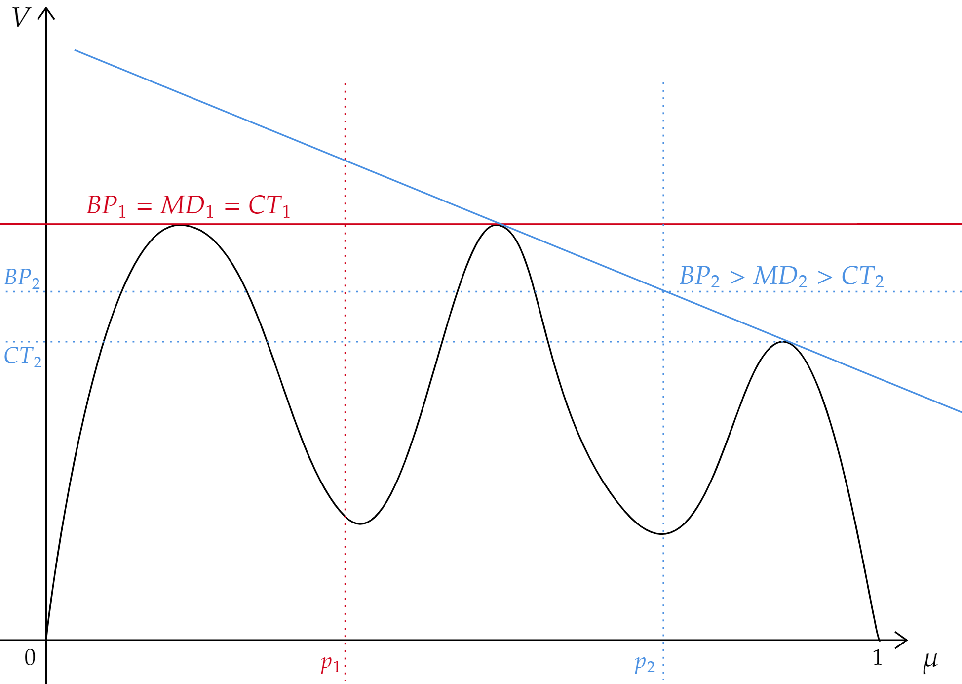
Figure 3: Flat vs. non-flat regression line

Figure 3 plots a singleton-valued $V$ with three peaks and illustrates both the case where the regression line is flat and the case where it is not. First, consider the prior $p_{1}$ between the first two equally high peaks of $V$. It is clear that the minimal affine function representing the concave envelope of $V$ at $p$ is the flat line passing through them. This coincides with their regression line and therefore the persuasion value can be attained with cheap talk. Differently, when we consider prior $p_{2}$ between the second and the third peaks with different values, the corresponding regression line for optimal persuasion is not flat, hence mediation cannot implement any persuasion-optimal distribution.

Proposition 2 implies that it suffices to focus on the pairwise comparison of persuasion vs. cheap talk and mediation vs. cheap talk. Geometrically, cheap talk attains the persuasion value if and only if the concave envelope and the quasiconcave envelope of $\mkern 2.0mu\overline{\mkern-2.0muV\mkern-2.0mu}\mkern 2.0mu$ coincide at $p$. When the state is binary, this happens if and only if cheap talk attains global maximum value, or no disclosure is optimal under persuasion (i.e., (iii) in Proposition 2).

Next, we present a geometric comparison between mediation and cheap talk. When $\Omega$ is binary, this comparison is captured by a weaker version of the single-crossing condition. Recall that given a closed-valued correspondence $\mathbf{U}:\mathbb{R}\rightrightarrows\mathbb{R}$, its upper and lower envelope respectively are $\mkern 2.0mu\overline{\mkern-2.0muU\mkern-2.0mu}\mkern 2.0mu(x)=\max\mathbf{U}(x)$ and $\mkern 2.0mu\underline{U\mkern-3.0mu}\mkern 3.0mu(x)=\min\mathbf{U}(x)$. A correspondence $\mathbf{U}$ is mono-crossing from below if for any $x<x^{\prime}$, $\mkern 2.0mu\overline{\mkern-2.0muU\mkern-2.0mu}\mkern 2.0mu(x)>0$ implies $\mkern 2.0mu\underline{U\mkern-3.0mu}\mkern 3.0mu(x^{\prime})\geq 0$. $\mathbf{U}$ is mono-crossing from above if for any $x<x^{\prime}$, $\mkern 2.0mu\underline{U\mkern-3.0mu}\mkern 3.0mu(x)<0$ implies $\mkern 2.0mu\overline{\mkern-2.0muU\mkern-2.0mu}\mkern 2.0mu(x^{\prime})\leq 0$. We say $\mathbf{U}$ is mono-crossing if it is mono-crossing either from below or from above. When $\mathbf{U}$ is singleton-valued, we obtain the corresponding definition for functions: See Figure 4.

Proposition 3.

If no disclosure is suboptimal under cheap talk, then $\mathcal{V}_{MD}(p)=\mathcal{V}_{CT}(p)$ if and only if $\mathbf{V}(\mu)-\mkern 2.0mu\overline{\mkern-2.0muV\mkern-2.0mu}\mkern 2.0mu_{CT}(p)$ is mono-crossing.

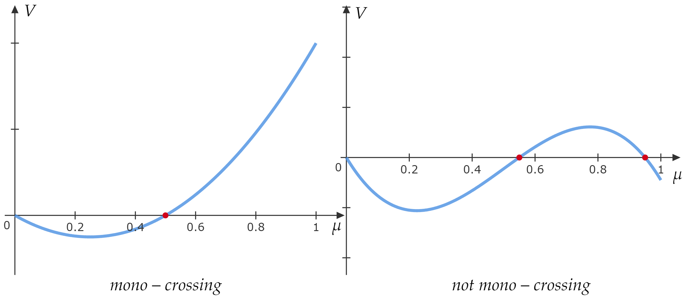
Figure 4: Comparison of mono-crossing and not mono-crossing functions

Intuitively, the mono-crossing condition captures the sender’s tendency to misreport. Fix any $V\in\mathbf{V}$ such that the shifted indirect utility $V(\mu)-\mkern 2.0mu\overline{\mkern-2.0muV\mkern-2.0mu}\mkern 2.0mu_{CT}(p)$ is mono-crossing and $V(p)<\mkern 2.0mu\overline{\mkern-2.0muV\mkern-2.0mu}\mkern 2.0mu_{CT}(p)$. We have $V(\mu)\leq\mkern 2.0mu\overline{\mkern-2.0muV\mkern-2.0mu}\mkern 2.0mu_{CT}(p)$ on at least one of $[0,p)$ or $(p,1]$. In the former case, the sender always prefers to over-claim the state if her preference is mono-crossing from below. Hence, it is impossible for the mediator to credibly randomize over the posteriors with sender values higher/lower than $\mathcal{V}_{CT}(p)$, which is the key for mediation to outperform cheap talk as we will show in Section 6.

If instead, no disclosure is optimal under cheap talk, then $\mathcal{V}_{MD}(p)=\mathcal{V}_{CT}(p)$ if and only if no disclosure is optimal under mediation. Applying the results in Dworczak and Kolotilin (2023), we may verify the optimality of no disclosure when $\mathbf{V}=V$ is singleton-valued. If there exists $g\in\mathbb{R}$ such that the distorted value function $(1+g(\mu-p))V(\mu)$ in Proposition 1 is superdifferentiable at $p$, then no disclosure is optimal under mediation.

When the sender’s payoff is uniquely defined given the receiver’s posterior and we strengthen the mono-crossing condition of Proposition 3 to the standard single-crossing condition, the equivalence between mediation and chap talk is much stronger as we show next.

Proposition 4.

Assume that $\mathbf{V}=V$ is singleton-valued. If $V(\mu)-\mkern 2.0mu\overline{\mkern-2.0muV\mkern-2.0mu}\mkern 2.0mu_{CT}(p)$ is single-crossing at $\mu=p$, then $\mathcal{T}_{MD}(p)=\mathcal{T}_{CT}(p)$ and all cheap talk equilibria attain the same value for the sender. In this case, no disclosure is optimal for mediation.

The assumptions of Proposition 4 hold whenever $\mathbf{V}=V$ is monotone. Therefore, countervailing incentives (i.e., $V$ non-monotone) are necessary for mediation to strictly outperform cheap talk with binary states.

Propositions 3 and 4 imply that cheap talk and mediation attain the same sender-optimal value for several canonical shapes of the sender’s payoff.

Corollary 3.

Assume that $\mathbf{V}=V$ is singleton-valued. If $V$ is concave or quasiconvex, then $\mathcal{V}_{MD}(p)=\mathcal{V}_{CT}(p)$ for all $p\in(0,1)$. There exists a non-monotone quasiconcave $V$ and $p\in(0,1)$ such that $\mathcal{V}_{MD}(p)>\mathcal{V}_{CT}(p)$.

When $V$ is concave, it is well known that $\mathcal{V}_{BP}(p)=V(p)$, hence all the three communication protocols yield the same value as no disclosure. When $V$ is quasiconvex, the shifted value $V(\mu)-\mkern 2.0mu\overline{\mkern-2.0muV\mkern-2.0mu}\mkern 2.0mu_{CT}(p)$ is either mono-crossing or single-crossing at $\mu=p$. When $V$ is quasiconcave, we cannot apply Proposition 3 since no disclosure is sender-optimal for cheap talk. However, we can still construct an example with a quasiconcave (yet not concave) indirect value $V$ and prior $p$ such that no disclosure is suboptimal for mediation.

In Sections 5 and 6, we generalize these results to settings with an arbitrary number of states. While the basic intuition remains the same, the higher dimensionality of the problem does not allow us to use one-dimensional notions such as the mono-crossing or single-crossing properties to characterize when elicitation and mediation are strictly valuable. However, these properties are still relevant when the sender’s payoff depends on a one-dimensional statistic of the receiver’s posterior (see Appendix C.2).

5 Persuasion vs. Mediation

In this section, we go back to our general setting and compare the sender’s optimal value under Bayesian persuasion and mediation. Our first result extends Proposition 2.

Theorem 2.

Elicitation has no value if and only if commitment has no value, that is,

$$\mathcal{V}_{BP}(p)=\mathcal{V}_{MD}(p)\Longleftrightarrow\mathcal{V}_{BP}(p)=\mathcal{V}_{CT}(p).$$

Theorem 2 implies there are only three possible relationships among the values: $\mathcal{V}_{BP}(p)=\mathcal{V}_{MD}(p)=\mathcal{V}_{CT}(p)$, $\mathcal{V}_{BP}(p)>\mathcal{V}_{MD}(p)=\mathcal{V}_{CT}(p)$, or $\mathcal{V}_{BP}(p)>\mathcal{V}_{MD}(p)>\mathcal{V}_{CT}(p)$. Combined with the geometric characterizations of the optimal persuasion value (Kamenica and Gentzkow (2011)) and the optimal cheap talk value (Lipnowski et al. (2022)), Theorem 2 also provides a geometric comparison between the sender’s optimal value under commitment and their optimal value under any truthful communication mechanism: these are the same if and only if the concave and quasiconcave envelopes of the sender’s value function coincide at the prior. Therefore, if the sender cannot achieve the optimal persuasion value using single-round cheap talk, then she cannot attain this via any communication mechanism without sender commitment (e.g. multiple-round cheap talk, noisy cheap talk).

The proof of Theorem 2 generalizes that of Proposition 2 to multiple states. In fact, the optimal persuasion value is still attained from above by the minimal affine functional (i.e., a hyperplane) that dominates $\mkern 2.0mu\overline{\mkern-2.0muV\mkern-2.0mu}\mkern 2.0mu(\mu)$ pointwise. Let $L_{p}(\mu)=\langle f_{p},\mu\rangle$ denote this affine functional, where $f_{p}\in\mathbb{R}^{n}$ is its representing vector, and fix a finitely supported distribution $\tau$ that is optimal under persuasion and that is implementable under mediation. The duality result in Dworczak and Kolotilin (2023) implies that $\mkern 2.0mu\overline{\mkern-2.0muV\mkern-2.0mu}\mkern 2.0mu(\mu)=\langle f_{p},\mu\rangle$ for all $\mu$ in the support of $\tau$. In other words, $f_{p}$ represents the regression hyperplane that passes through all the points $\left\{(\mu,\mkern 2.0mu\overline{\mkern-2.0muV\mkern-2.0mu}\mkern 2.0mu(\mu))\right\}_{\mu\in\operatorname{supp}(\tau)}$. The zeroCov condition of Theorem 1 implies that there exists an intercept $\alpha\in\mathbb{R}$ such that $\mkern 2.0mu\overline{\mkern-2.0muV\mkern-2.0mu}\mkern 2.0mu(\mu)=\langle f_{p},\mu\rangle=\alpha$ for all $\mu\in\operatorname{supp}(\tau)$. Therefore, $\tau$ must be implementable under cheap talk because it induces a constant optimal value for the sender, hence $\mathcal{V}_{BP}(p)=\mathcal{V}_{CT}(p)$.

Unlike the binary case, comparing the concave envelope and the quasiconcave envelope is not easy in general. Thus, we take a constructive approach and provide a sufficient condition for persuasion to strictly outperform mediation. To state the formal condition, we begin with the following definition. We say a distribution $\tau\in\mathcal{T}_{CT}(p)$ attains value $s$ (under cheap talk) if $s\in\cap_{\mu\in\operatorname{supp}(\tau)}\mathbf{V}(\mu)$, and a value $s\in\mathbb{R}$ is attainable under cheap talk if there exists $\tau\in\mathcal{T}_{CT}(p)$ that attains it. By Theorem 1 in Lipnowski and Ravid (2020), $s\geq\mkern 2.0mu\overline{\mkern-2.0muV\mkern-2.0mu}\mkern 2.0mu(p)$ is attainable under cheap talk if and only if $p\in\operatorname*{co}\left\{\mu\in\Delta(\Omega):\mkern 2.0mu\overline{\mkern-2.0muV\mkern-2.0mu}\mkern 2.0mu(\mu)\geq s\right\}$. For every set $D\subseteq\Delta(\Omega)$, let $\operatorname*{aff}(D)\subseteq\mathbb{R}^{n}$ denote the affine hull of $D$.

Definition 2.

For every $s\geq\mkern 2.0mu\overline{\mkern-2.0muV\mkern-2.0mu}\mkern 2.0mu(p)$ attainable under cheap talk, we define the cheap talk hull of $s$ as

$$H(s)\coloneqq\bigcup\left\{\operatorname*{aff}(\operatorname{supp}(\tau))\cap\Delta(\Omega):\tau\in\mathcal{T}_{CT}(p)\textnormal{ attains value }s,\,|\operatorname{supp}(\tau)|<\infty\right\}.$$ (1)

We define $H^{*}\coloneqq H(\mathcal{V}_{CT}(p))$.

The cheap talk hull of $s$ is the intersection of $\Delta(\Omega)$ and the largest affine hull spanned by the support of some $\tau\in\mathcal{T}_{CT}(p)$ with finite support. In this case, we say that $\tau$ spans out $H(s)$.

Theorem 2 leads to the following sufficient condition for persuasion to strictly outperform mediation – it suffices to check whether there exists another $\mu\in H^{*}$ where the sender’s most preferred cheap talk equilibrium with prior $\mu$ is strictly better than the optimal cheap talk equilibrium with prior $p$.

Proposition 5.

If there exists $\mu\in H^{*}$ such that $\mkern 2.0mu\overline{\mkern-2.0muV\mkern-2.0mu}\mkern 2.0mu_{CT}(\mu)>\mkern 2.0mu\overline{\mkern-2.0muV\mkern-2.0mu}\mkern 2.0mu_{CT}(p)$, then $\mathcal{V}_{BP}(p)>\mathcal{V}_{MD}(p)$.

The proof is constructive. Fix any optimal $\tau\in\mathcal{T}_{CT}(p)$ that spans out $H^{*}$. For any posterior $\mu\in H^{*}$ with $\mkern 2.0mu\overline{\mkern-2.0muV\mkern-2.0mu}\mkern 2.0mu_{CT}(\mu)>\mkern 2.0mu\overline{\mkern-2.0muV\mkern-2.0mu}\mkern 2.0mu_{CT}(p)$, there exists $\tau_{\mu}\in\mathcal{T}_{CT}(\mu)$ that attains $\mkern 2.0mu\overline{\mkern-2.0muV\mkern-2.0mu}\mkern 2.0mu_{CT}(\mu)$ and $\alpha_{\mu}>1$ such that $(1-\alpha_{\mu})\mu+\alpha_{\mu}p$ is in the (relative) interior of $\operatorname*{co}(\operatorname{supp}(\tau))$. Hence, there exists $\tau^{\prime}\in\mathcal{T}_{CT}((1-\alpha_{\mu})\mu+\alpha_{\mu}p)$ that attains $\mkern 2.0mu\overline{\mkern-2.0muV\mkern-2.0mu}\mkern 2.0mu_{CT}(p)$, and $\tfrac{1}{\alpha_{\mu}}\tau^{\prime}+\tfrac{\alpha_{\mu}-1}{\alpha_{\mu}}\tau_{\mu}$ is a distribution of beliefs centered at prior $p$ and that attains a value strictly higher than $\mkern 2.0mu\overline{\mkern-2.0muV\mkern-2.0mu}\mkern 2.0mu_{CT}(p)$. This construction also yields a lower bound on the value of commitment:

$$\mathcal{V}_{BP}(p)-\mathcal{V}_{CT}(p)\geq\tfrac{\alpha_{\mu}-1}{\alpha_{\mu}}(\mkern 2.0mu\overline{\mkern-2.0muV\mkern-2.0mu}\mkern 2.0mu_{CT}(\mu)-\mkern 2.0mu\overline{\mkern-2.0muV\mkern-2.0mu}\mkern 2.0mu_{CT}(p)).$$

for all $\mu\in H^{*}$ such that $\mkern 2.0mu\overline{\mkern-2.0muV\mkern-2.0mu}\mkern 2.0mu_{CT}(\mu)>\mkern 2.0mu\overline{\mkern-2.0muV\mkern-2.0mu}\mkern 2.0mu_{CT}(p)$.

We next introduce an important particular case that will help us to make tighter the comparison between persuasion and mediation in this section and the one between cheap talk and mediation in the next section.

Definition 3.

We say that the full-dimensionality condition holds at $p$ if $H^{*}=\Delta(\Omega)$.

Full-dimensionality amounts to having a solution of the cheap talk program that spans out the entire simplex. Moreover, it allows us to make the condition of Proposition 5 tight.

Corollary 4.

Assume that the full-dimensionality condition holds at $p$. Then, $\mathcal{V}_{BP}(p)>\mathcal{V}_{MD}(p)$ if and only if there exists $\mu\in\Delta(\Omega)$ such that $\mkern 2.0mu\overline{\mkern-2.0muV\mkern-2.0mu}\mkern 2.0mu(\mu)>\mkern 2.0mu\overline{\mkern-2.0muV\mkern-2.0mu}\mkern 2.0mu_{CT}(p)$.

When does the full-dimensionality condition hold? In the binary-state case, it holds if the maximum cheap talk value is strictly higher than the maximum value achievable under no disclosure. In general, the next lemma exactly answers the previous question by characterizing the full-dimensionality condition in terms of the value that the sender can attain under cheap talk around the prior.

Lemma 1.

The full-dimensionality condition holds at $p$ if and only if $\mkern 2.0mu\overline{\mkern-2.0muV\mkern-2.0mu}\mkern 2.0mu_{CT}(p)$ can be attained under cheap talk at every prior in an open neighborhood of $p$. In particular, the full-dimensionality condition holds if $\mkern 2.0mu\overline{\mkern-2.0muV\mkern-2.0mu}\mkern 2.0mu_{CT}$ is locally constant around $p$.

This characterization is particularly useful because $\mkern 2.0mu\overline{\mkern-2.0muV\mkern-2.0mu}\mkern 2.0mu_{CT}$ is locally constant around $p$ for almost every prior $p$ when the action set $A$ is finite, as shown in Corollary 2 of Lipnowski and Ravid (2020). Combining this observation with our Corollary 4 yields that, when the action set is finite, for almost all priors, either cheap talk achieves the global maximum value or elicitation is strictly valuable.

5.1 The Think Tank Revisited

We now illustrate the ideas introduced in this section with a three-state example. Think tanks often act as research mediators between an interest group and lawmakers. In particular, the most prominent ones have enough reputation to make a credible commitment to information policies that elicit information from an interest group and release it to the lawmaker. Here, we revisit the think-tank example in Lipnowski and Ravid (2020) by assuming that the sender is an interest group, say a lobbyist with private knowledge of the state, the receiver is a lawmaker with the option to maintain the status quo or to choose a new policy, and the mediator is a think tank which is completely aligned to the interest group.

There are three possible states of the world $\Omega=\{\omega_{1},\omega_{2},\omega_{3}\}$ and the lawmaker can take one of four actions $A=\{a_{0},a_{1},a_{2},a_{3}\}$. Each action $a_{i}$ for $i\in\left\{1,2,3\right\}$ represents a costly and risky policy that pays if and only if the state is $\omega_{i}$. Differently, action $a_{0}$ is safe and represents the status quo. Formally, the lawmaker’s payoff $u_{R}(\omega_{i},a_{j})$ is $1$ if $i=j\neq 0$, $0$ if $j=0$, and $-c$ otherwise for some $c>1$.

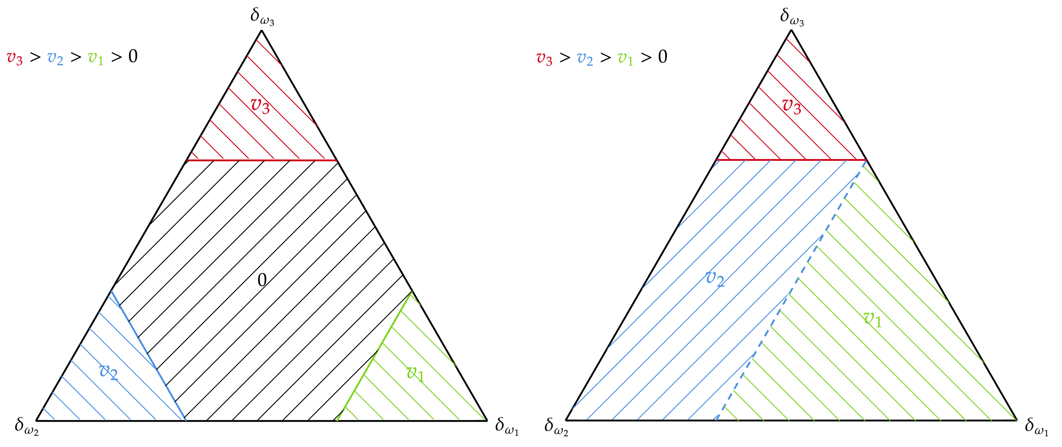
Figure 5: Lobbyist’s value function and its quasiconcave envelope

Left panel: lobbyist’s value correspondence over the lawmaker’s belief space. Right panel: lobbyist’s optimal cheap talk value (i.e., quasiconcave envelope) over the lawmaker’s belief space. This illustrates the case where $c=2$.

The lobbyist is informed about the state of the world, but their preferences are misaligned with respect to the lawmaker. In particular, the lobbyist’s payoff is $u_{S}(a)=\sum_{i=0}^{3}v_{i}\mathbb{I}[a=a_{i}]$ with $v_{3}>v_{2}>v_{1}>v_{0}=0$, that is, the lobbyist prefers higher indexed policies and maintaining the status quo yields zero payoff. Therefore, the lobbyist wants to influence the lawmaker to change the status quo regardless of the state of the world.

Given belief $\mu\in\Delta(\Omega)$, the lawmaker’s best response is to take action $a_{i}$ if and only if $\mu(\omega_{i})>\tfrac{c}{1+c}$, and they are indifferent between $a_{i}$ and $a_{0}$ when $\mu(\omega_{i})=\tfrac{c}{1+c}$. This is illustrated in the left panel of Figure 5. The colored regions at the vertexes of the simplex represent the beliefs such that the lobbyist’s payoff is equal to $v_{i}$ for some $i\in\left\{1,2,3\right\}$. The central hexagon is the region of the lawmaker’s beliefs where their optimal response is to maintain the status quo, yielding a zero payoff for the lobbyist. Observe that the boundary segments between each colored region and the zero-payoff region represent the beliefs such that the lawmaker is indifferent between the status quo and one of the new policies.

Suppose first that the lobbyist communicates with the lawmaker without the think tank mediation. This corresponds to the cheap-talk case and the lobbyist’s optimal value as a function of the prior belief $p$ is

$$\mathcal{V}_{CT}(p)=\begin{cases}v_{3}&\text{if }p(\omega_{3})\geq\tfrac{c}{1+c}\\ v_{1}&\text{if }p(\omega_{1})\geq\tfrac{1}{1+c}\\ v_{2}&\text{otherwise}.\end{cases}$$

This is the quasiconcave envelope $\mkern 2.0mu\overline{\mkern-2.0muV\mkern-2.0mu}\mkern 2.0mu_{CT}(p)$ of $\mkern 2.0mu\overline{\mkern-2.0muV\mkern-2.0mu}\mkern 2.0mu$ evaluated at $p$. The right panel of Figure 5 shows the level sets of the quasiconcave envelope over the simplex. When the prior is in one of the three colored regions in the left panel, then the babbling equilibrium is optimal for the lobbyist. Instead, the status-quo region can be split into two subregions. For priors that lie between the $v_{2}$ and $v_{3}$ regions, there exists an equilibrium distribution of the lawmaker’s beliefs supported on posteriors where $a_{2}$ is uniquely optimal and posteriors where the lawmaker is indifferent between the status quo and $a_{3}$. Differently, for priors to the right of the blue dashed line, (BP) implies that any optimal equilibrium must induce at least a posterior where $a_{1}$ is optimal, implying the highest value attainable is $v_{1}$.

Given that the action set is finite, the full-dimensionality condition holds at almost all priors $p$ in the simplex. For example, suppose that the prior $p$ lies between the $v_{2}$ and $v_{3}$ region as in Figure 6. Around this prior, the quasiconcave envelope $\mkern 2.0mu\overline{\mkern-2.0muV\mkern-2.0mu}\mkern 2.0mu_{CT}$ is constant and equal to $v_{2}$. For instance, this value is attained by the lobbyist-optimal distribution of the lawmaker’s beliefs supported over $\left\{\mu_{1},\mu_{2},\mu_{3},\mu_{4}\right\}$ as shown in Figure 6. At posteriors $\mu_{2}$ and $\mu_{3}$ the lawmaker takes action $a_{2}$, whereas on $\mu_{1}$ and $\mu_{4}$ the lawmaker mixes between the status quo and action $a_{3}$ so to induce exactly a payoff equal to $v_{2}$ for the lobbyist. Observe that the affine hull of $\left\{\mu_{1},\mu_{2},\mu_{3},\mu_{4}\right\}$ has dimension 2, hence full dimensionality holds.

Figure 6: Construction of a cheap-talk equilibrium distribution of beliefs with a full-dimensional cheap talk hull.

Assume now that the lobbyist and the lawmaker communicate through the mediation of the think tank. We can easily apply Corollary 4 to establish when the think tank mediation secures to the lobbyist the Bayesian persuasion value. In fact, this happens if and only if the prior lies in the $v_{3}$ region, i.e., the red triangle in the left panel of Figure 5. In this case, no disclosure is optimal for all three of the communication protocols considered. As soon as the prior $p$ is outside this region, that is when $p(\omega_{3})<\tfrac{c}{1+c}$, we have $\mkern 2.0mu\overline{\mkern-2.0muV\mkern-2.0mu}\mkern 2.0mu_{CT}(\mu)>\mkern 2.0mu\overline{\mkern-2.0muV\mkern-2.0mu}\mkern 2.0mu_{CT}(p)$ for all $\mu$ in the $v_{3}$ region, yielding that $\mathcal{V}_{BP}(p)>\mathcal{V}_{MD}(p)\geq\mathcal{V}_{CT}(p)$.

For example, for the prior $p$ considered in Figure 6, we can still consider the distribution over posteriors supported on $\left\{\mu_{1},\mu_{2},\mu_{3},\mu_{4}\right\}$ but this time selecting a different best response for the lawmaker: $a_{2}$ at $\mu_{2}$ and $\mu_{3}$, and $a_{3}$ at $\mu_{1}$ and $\mu_{4}$. This distribution does not correspond to any cheap talk equilibrium but can be induced by committing to some information structure. Given Theorem 2, both cheap talk and mediation are outperformed in this case. Overall, this shows that, for a large set of prior beliefs, a lobbyist with commitment power would be strictly better off than the case where they communicate through an uninformed think tank with commitment, that is, the value of elicitation is often strictly positive.

6 Mediation vs. Cheap Talk

In this section, we offer a general comparison between the sender’s optimal value under mediation and under cheap talk. In particular, we will provide separate sufficient and necessary conditions for the mediator to strictly outperform direct communication by introducing some randomness. Moreover, these conditions collapse under the full-dimensionality condition introduced in the previous section, yielding a tight geometric characterization of when mediation is strictly valuable.

We start with a useful lemma that extends Theorem 1 in Lipnowski and Ravid (2020).

Lemma 2.

For every $s\in\mathbb{R}$, $\mkern 2.0mu\overline{\mkern-2.0muV\mkern-2.0mu}\mkern 2.0mu_{CT}(p)>s$ if and only if $p\in\operatorname*{co}\{\mkern 2.0mu\overline{\mkern-2.0muV\mkern-2.0mu}\mkern 2.0mu>s\}$, and $\mkern 2.0mu\underline{V\mkern-3.0mu}\mkern 3.0mu_{CT}(p)<s$ if and only if $p\in\operatorname*{co}\{\mkern 2.0mu\underline{V\mkern-3.0mu}\mkern 3.0mu<s\}$.

This lemma implies that there exists a cheap talk equilibrium that attains a strictly higher (lower) value than $s$ if and only if the prior lies in the convex hull of posteriors with highest (lowest) value strictly above (below) $s$.

As we have seen in Corollary 2, the mediator must randomize to strictly improve on cheap talk. Here, we show that they must randomize over posteriors with a value strictly above and below the optimal cheap talk value. Recall that the cheap talk hull $H(s)$ of $s$ is defined in (1).

Definition 4.

For any $s\geq\mkern 2.0mu\overline{\mkern-2.0muV\mkern-2.0mu}\mkern 2.0mu(p)$ attainable under cheap talk, we say that $s$ is (locally) improvable at $p$ if there exist $\mu\in\Delta(\Omega)$ ($\mu\in H(s)$) and $\lambda\in[0,1)$ such that

$$\mkern 2.0mu\overline{\mkern-2.0muV\mkern-2.0mu}\mkern 2.0mu_{CT}(\lambda\mu+(1-\lambda)p)>s>\mkern 2.0mu\underline{V\mkern-3.0mu}\mkern 3.0mu_{CT}(\mu).$$

We say that cheap talk is (locally) improvable at $p$ if $\mathcal{V}_{CT}(p)$ is (locally) improvable at $p$.

In words, $s$ is locally improvable at $p$ if there are alternative priors $\mu\in H(s)$ and $\mu^{\prime}=\lambda\mu+(1-\lambda)p$ such that there exists a cheap talk equilibrium at $\mu$ and one at $\mu^{\prime}$ that respectively yield a strictly lower and a strictly higher expected payoff to the sender. Importantly, the prior $\mu^{\prime}$ corresponding to the high-value equilibrium has to be “closer” to the original prior $p$, in the sense that $\mu^{\prime}$ lies in the semi-open segment $[p,\mu)$.

We can now state the main result of this section.

Theorem 3.

For any $s\geq\mkern 2.0mu\overline{\mkern-2.0muV\mkern-2.0mu}\mkern 2.0mu(p)$ attainable under cheap talk, if $s$ is locally improvable at $p$, then $\mathcal{V}_{MD}(p)>s$. Conversely, if $s$ is not improvable at $p$, then $\mathcal{V}_{MD}(p)=s$.

As for Proposition 5, the proof of the first statement is constructive, and it is graphically illustrated in Figure 7 in subsection 6.1. If $s$ is locally improvable at $p$, then there exists $\mu_{-}\in H(s)$ and $\mu_{+}\in[p,\mu_{-})$ and two cheap talk equilibria $\tau_{-}$ and $\tau_{+}$ respectively centered at $\mu_{-}$ and $\mu_{+}$ that attain a value strictly lower and strictly higher than $s$. Because $\mu_{-}\in H(s)$, there exists $\mu_{0}$ that lies on the half line with endpoint $\mu_{-}$ through $p$, such that $s$ can be attained by a cheap talk equilibrium $\tau_{0}$ centered at $\mu_{0}$. The mediator may then randomize over three cheap talk equilibria $\tau_{+},\tau_{-}$ and $\tau_{0}$ such that (BP) and (TT) are satisfied, which reduces to a 1-dimensional problem as the barycenters are colinear. Since $\mu_{+}$ is “closer” to the prior $p$ compared to $\mu_{-}$, (TT) requires the mediator to assign a relatively higher weight to $\tau_{+}$ compared to $\tau_{-}$, so the sender’s expected utility is strictly higher than $s$ with this randomization. Note that this construction also provides a lower bound on the value of mediation, which depends on the barycenters and cheap talk equilibria in the construction.

The proof of the converse statement is more technical. Suppose $s$ is not improvable at $p$, then there exists a hyperplane $H$ that properly separates all posteriors with values strictly higher than $s$ from those with values strictly lower than $s$. Moreover, the prior $p$ lies in the same closed half-space as the posteriors with a value strictly below $s$. A normal vector $g\in\mathbb{R}^{n}$ of $H$ is a Lagrange multiplier for the (TT) constraint such that $(V(\mu)-s)\langle g,\mu\rangle\leq 0$ for any $V\in\mathbf{V}$. Hence, for any $(\tau,V)$ implementable under mediation, we have

$$0\geq\int(V(\mu)-s)\langle g,\mu\rangle\mathop{}\!\mathrm{d}\tau(\mu)=\left(\int V(\mu)\mathop{}\!\mathrm{d}\tau(\mu)-s\right)\langle g,p\rangle,$$

by (zeroCov) and (BP). When $p$ does not lie on $H$, we conclude that $\int V\mathop{}\!\mathrm{d}\tau\leq s$. Otherwise, $\tau$ can be supported on posteriors such that $V(\mu)\neq s$ only if $\mu\in H\cap\Delta(\Omega)$, which is a strictly lower-dimensional set. We can find another separating hyperplane $H^{\prime}$ while restricting attention to $H\cap\Delta(\Omega)$ and then repeat the same argument until $p$ is not in the separating hyperplane or until the intersection of all separating hyperplanes $H\cap H^{\prime}\cap\Delta(\Omega)$ is a singleton ${p}$. Either case leads to the desired conclusion that $\mathcal{V}_{MD}(p)\leq s$.

Paralleling the analysis in Section 5, under full dimensionality the previous result yields a complete geometric characterization of the case when mediation is strictly valuable.

Corollary 5.

The following hold:

1. If cheap talk is locally improvable at $p$, then $\mathcal{V}_{MD}(p)>\mathcal{V}_{CT}(p)$ and every optimal distribution of beliefs under mediation is induced by a random communication mechanism.

2. Conversely, if cheap talk is not improvable at $p$, then $\mathcal{V}_{MD}(p)=\mathcal{V}_{CT}(p)$.

Moreover, if the full-dimensionality condition holds at $p$, then $\mathcal{V}_{MD}(p)>\mathcal{V}_{CT}(p)$ if and only if cheap talk is improvable at $p$.

The first two statements of the corollary immediately follow by taking $s=\mathcal{V}_{CT}(p)$ in Theorem 3. For the last part of the corollary, full dimensionality implies that cheap talk is locally improvable at $p$ if and only if it is improvable at $p$, hence the necessary and sufficient conditions of the first part collapse. In general, full dimensionality holds when the quasiconcave envelope $\mkern 2.0mu\overline{\mkern-2.0muV\mkern-2.0mu}\mkern 2.0mu_{CT}(p)$ is locally flat at $p$ (see Lemma 1), which is the case for almost every prior $p$ when the action set $A$ is finite.

When the sender’s payoff correspondence is singleton-valued and no disclosure is not a sender’s optimal cheap talk equilibrium, it is possible to simplify the characterization of Corollary 5 as follows.

Corollary 6.

Assume that $\mathbf{V}=V$ is singleton-valued, that the full-dimensionality condition holds at $p$, and that no disclosure is suboptimal for cheap talk at $p$ (i.e., $\mkern 2.0mu\overline{\mkern-2.0muV\mkern-2.0mu}\mkern 2.0mu_{CT}(p)>V(p)$). Then $\mathcal{V}_{MD}(p)>\mathcal{V}_{CT}(p)$ if and only if there exists $\mu\in\Delta(\Omega)$ such that

$$\mkern 2.0mu\overline{\mkern-2.0muV\mkern-2.0mu}\mkern 2.0mu_{CT}(\mu)>\mkern 2.0mu\overline{\mkern-2.0muV\mkern-2.0mu}\mkern 2.0mu_{CT}(p)>\mkern 2.0mu\underline{V\mkern-3.0mu}\mkern 3.0mu_{CT}(\mu).$$

In this case, it is sufficient to find a single alternative prior $\mu$ that admits two cheap talk equilibria respectively inducing a strictly higher and a strictly lower sender’s payoff than the sender’s optimal cheap talk value at $p$.

The next remark discusses the effect of the sender’s preferred mediated communication on the receiver’s expected payoff.

Remark 1.

Theorem 3 and Corollary 5 provide sufficient and necessary conditions that ensure the value of mediation is strictly positive for the sender. It is then natural to ask whether mediation also improves the expected utility of the receiver, $\int V_{R}(\mu)d\tau(\mu)$, where $V_{R}(\mu):=\max_{a\in A}\mathbb{E}_{\mu}[u_{R}(\omega,a)]$ is the receiver’s utility given posterior $\mu$. By inspection of the proof of Theorem 3, it is easy to see that the distribution of beliefs $\tau\in\mathcal{T}_{MD}(p)$ that we construct to improve the sender’s expected utility would also strictly improve the receiver’s expected utility provided that $\mathbf{V}=V$ is singleton-valued and that $V_{R}(\mu)=G(V(\mu))$ for some strictly increasing and convex function $G:\mathbb{R}\to\mathbb{R}$. In general, it is not always easy to adapt our approach to conclude whether there exists a mediation plan that improves both the sender’s and receiver’s expected payoff compared to their payoffs under some sender-preferred cheap talk equilibrium. However, this is the case in the illustrative example in the introduction as well as in the illustrations in Sections 6.1 and 7.1.2.

Finally, we can use Theorem 3 to provide sufficient and necessary conditions for the optimality of full disclosure under mediation. Observe that full disclosure is feasible under cheap talk, or equivalently under mediation, if and only if there exists $s\in\mathbb{R}$ such that $s\in\cap_{\omega\in\Omega}\mathbf{V}(\delta_{\omega})$.

Corollary 7.

Full disclosure is optimal under mediation if and only if there exists $s\geq\mkern 2.0mu\overline{\mkern-2.0muV\mkern-2.0mu}\mkern 2.0mu(p)$ such that $s\in\cap_{\omega\in\Omega}\mathbf{V}(\delta_{\omega})$ and $s$ is not improvable at $p$. In this case, $\mathcal{V}_{MD}(p)=\mathcal{V}_{CT}(p)$.

The if part immediately follows from Theorem 3. Conversely, if full disclosure is optimal under mediation, it follows that $H^{*}=\Delta(\Omega)$, that is, full dimensionality holds. Therefore, the expected payoff induced by full disclosure cannot be improvable by Corollary 5.

6.1 Valuable Mediation in the Think-Tank Example

Consider again the setting of Section 5.1 with a lobbyist (sender) trying to influence a lawmaker (receiver) through a think tank (mediator). Here, we use the results of this section to show when the mediation of the think tank is strictly valuable. Recall that in this case, the full dimensionality condition holds at almost every prior.

Suppose first that the prior $p$ lies between the $v_{2}$ and $v_{3}$ region as in Figure 6. Observe that the lawmaker’s beliefs $\mu^{\prime}$ such that $\mkern 2.0mu\overline{\mkern-2.0muV\mkern-2.0mu}\mkern 2.0mu_{CT}(\mu^{\prime})>\mkern 2.0mu\overline{\mkern-2.0muV\mkern-2.0mu}\mkern 2.0mu_{CT}(p)=v_{2}$ are those in the $v_{3}$ region (i.e., the red triangle). Therefore, it is not possible to find a belief $\mu$ and a point $\mu^{\prime}$ in the segment $[p,\mu)$ as described in Definition 4. To see this, note that if $\mkern 2.0mu\overline{\mkern-2.0muV\mkern-2.0mu}\mkern 2.0mu_{CT}(\mu^{\prime})>v_{2}$ for some $\mu^{\prime}\in[p,\mu)$, then $\mu$ must be in the $v_{3}$ region except the boundary red line where the lobbyist is indifferent between $a_{3}$ and $a_{0}$, yielding that $\mkern 2.0mu\underline{V\mkern-3.0mu}\mkern 3.0mu_{CT}(\mu)=\mkern 2.0mu\overline{\mkern-2.0muV\mkern-2.0mu}\mkern 2.0mu_{CT}(\mu)=v_{3}$. This logic holds for all priors $p$ that are in the central hexagon and at the left of the dashed blue line in Figure 6, that is for any $p$ with $p(\omega_{1})<\tfrac{1}{1+c}$. For all such priors, cheap talk is not improvable at $p$, so the think tank is worthless in this case.

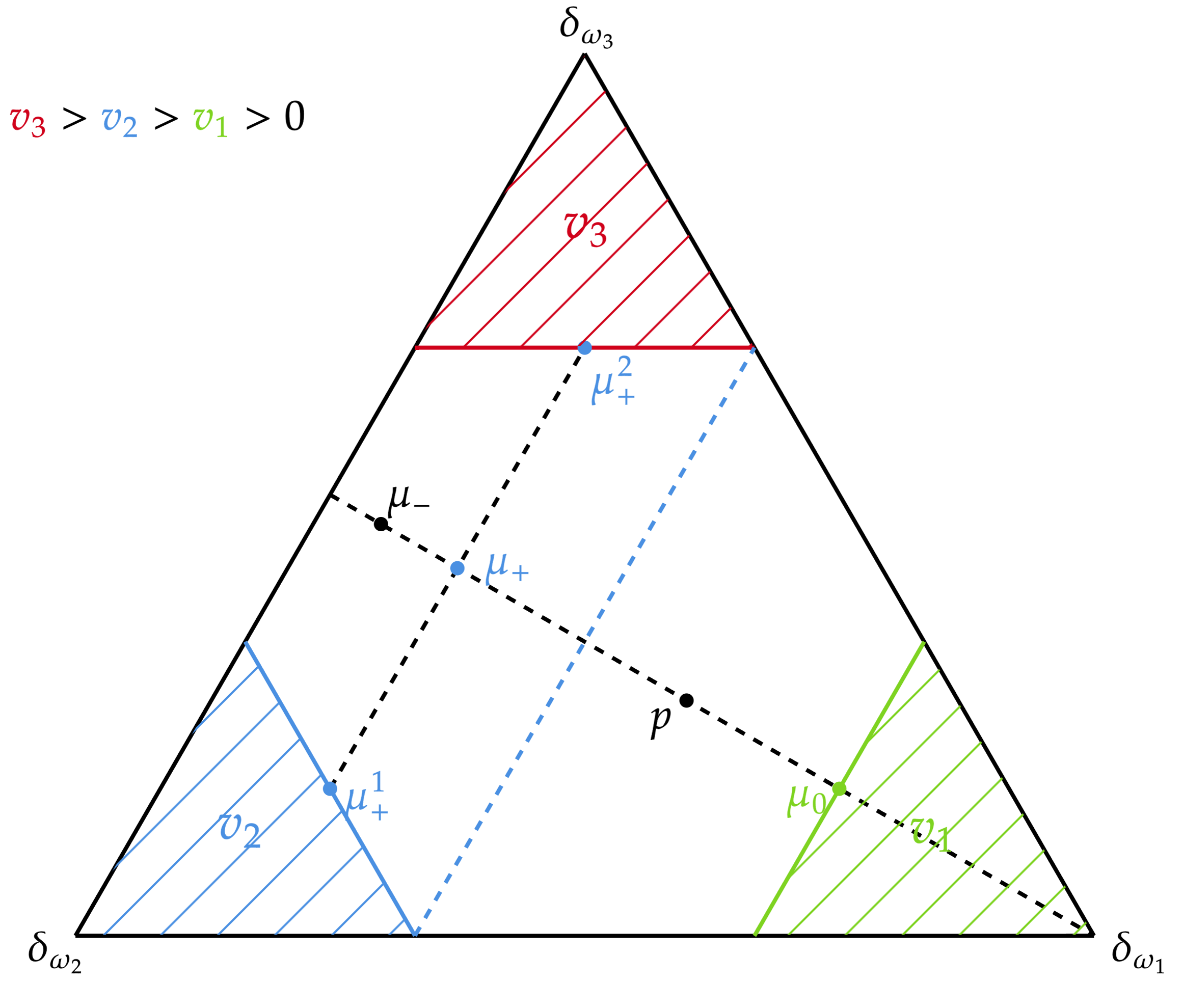
Figure 7: Construction of an improving distribution of beliefs under mediation

Differently, consider a prior $p$ to the right of the same dashed blue line as in Figure 7, that is such that $p(\omega_{1})>\tfrac{1}{1+c}$. At all these priors, cheap talk is improvable, so by Corollary 5 mediation by a think tank strictly improves upon direct communication. Intuitively, mediation helps strictly when the lawmaker has a pessimistic prior belief. Figure 7 graphically constructs an improving distribution of beliefs that is feasible under mediation following the logic of Theorem 3. First, recall from Figure 5 that $\mkern 2.0mu\overline{\mkern-2.0muV\mkern-2.0mu}\mkern 2.0mu_{CT}(p)=v_{1}>0$. Next, fix $\mu_{-}$ and $\mu_{+}\in[p,\mu_{-})$ lying in the same segment as in Figure 7. Both these two beliefs are to the left of the blue dashed line, implying that $\mkern 2.0mu\overline{\mkern-2.0muV\mkern-2.0mu}\mkern 2.0mu_{CT}(\mu_{+})=\mkern 2.0mu\overline{\mkern-2.0muV\mkern-2.0mu}\mkern 2.0mu_{CT}(\mu_{-})=v_{2}>v_{1}$. Moreover, $\mkern 2.0mu\underline{V\mkern-3.0mu}\mkern 3.0mu_{CT}(\mu_{-})=\mkern 2.0mu\underline{V\mkern-3.0mu}\mkern 3.0mu_{CT}(\mu_{+})=0$, the payoff of the babbling equilibrium. This shows that cheap talk is improvable at $p$. Next, consider a distribution $\tau_{+}$ of the lawmaker’s beliefs that is supported on $\left\{\mu^{1}_{+},\mu^{2}_{+}\right\}$ and with barycenter $\mu_{+}$. This is a feasible distribution of beliefs under cheap talk at prior $\mu_{+}$ since we can select a lawmaker’s mixed best response at $\mu^{2}_{+}$ that induces expected payoff $v_{2}$ for the lobbyist. Importantly, this distribution of beliefs and selection gives an overall expected payoff $\mkern 2.0mu\overline{\mkern-2.0muV\mkern-2.0mu}\mkern 2.0mu_{CT}(\mu_{+})=v_{2}>v_{1}$ to the lobbyist. Consider also two degenerate distributions of beliefs $\tau_{-}=\delta_{\mu_{-}}$ and $\tau_{0}=\delta_{\mu_{0}}$, where $\mu_{0}$ lies at the intersection of the previous segment and the boundary between the status-quo region and the $v_{1}$ region. Given that their barycenters all lie in the same segment as $p$, we can mix the three distributions of beliefs $\tau_{+},\tau_{-}$, and $\tau_{0}$ in a way to satisfy (BP) and (TT) while strictly improving the overall expected payoff of the lobbyist. Given that the barycenters of these distributions are colinear, the randomization over $\tau_{+},\tau_{-}$, and $\tau_{0}$ is the same as the one in the illustrative example in the introduction.

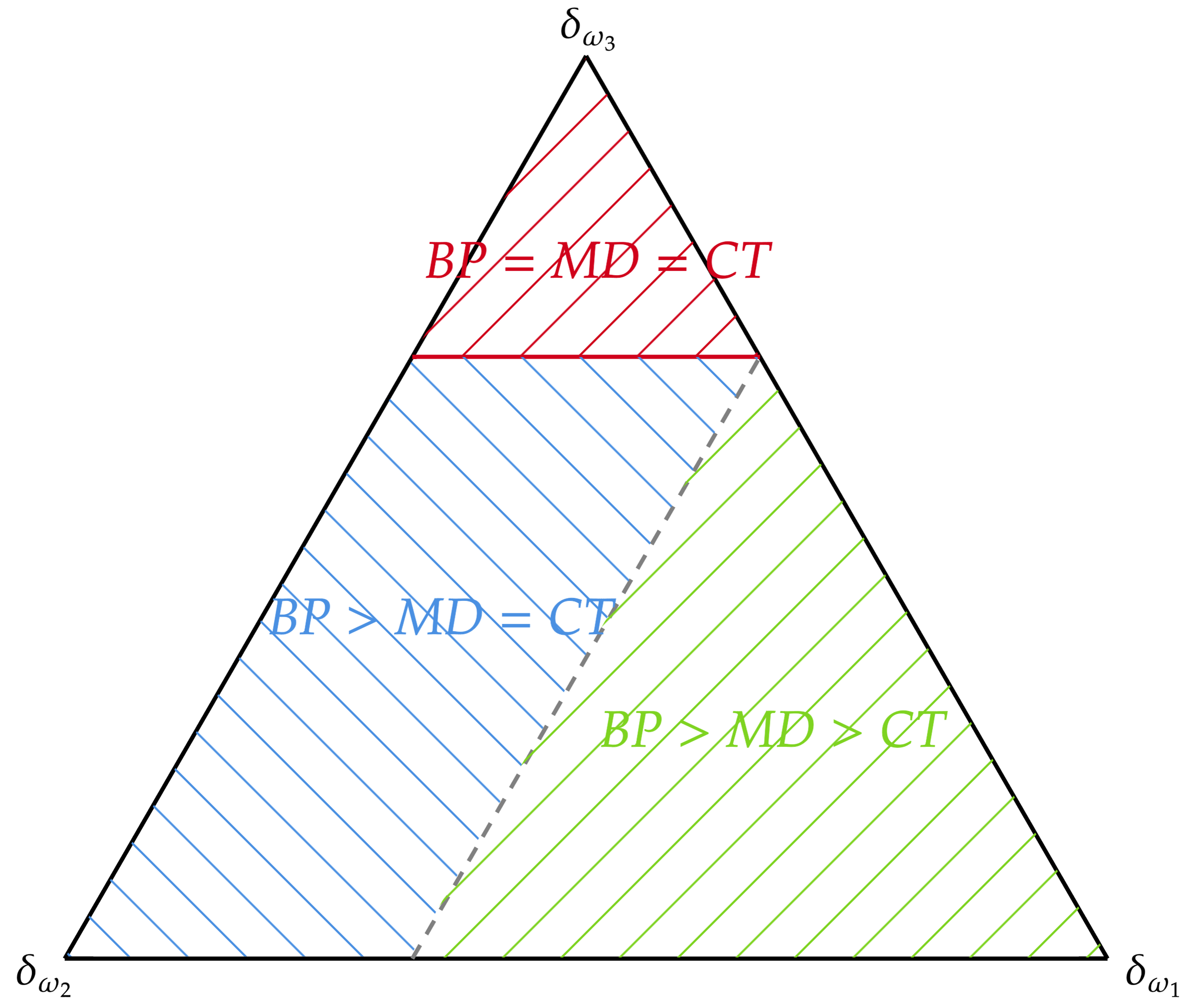
Figure 8: Relationships among communication protocols

For $p$ with $p(\omega_{1})\geq\tfrac{c}{1+c}$, no disclosure is optimal under cheap talk and suboptimal under mediation. Hence, the optimal mediation solution is strictly more informative than an optimal cheap talk equilibrium under these priors. Moreover, as the cost $c$ increases, the region where the cheap talk is improvable expands, and it converges to the entire simplex as $c\to\infty$. Therefore, mediation by a think tank is more likely to be valuable for high-stakes decisions. In general, the dotted blue line in Figure 7 separates the status-quo hexagon into two regions: to its left elicitation is strictly valuable but mediation is not, to its right both elicitation and mediation are strictly valuable. The relations among the three protocols are summarized in Figure 8. All the three possible scenarios that we mentioned after Theorem 2 are present in the current example: For priors $p$ in the red region we have $\mathcal{V}_{BP}(p)=\mathcal{V}_{MD}(p)=\mathcal{V}_{CT}(p)$, for $p$ in the blue region $\mathcal{V}_{BP}(p)>\mathcal{V}_{MD}(p)=\mathcal{V}_{CT}(p)$, and for $p$ in the green region $\mathcal{V}_{BP}(p)>\mathcal{V}_{MD}(p)>\mathcal{V}_{CT}(p)$.

Finally, we show that for every $p$ such that $p(\omega_{1})\in(\tfrac{1}{1+c},\tfrac{c}{1+c})$, there is a distribution of beliefs $\tau\in\mathcal{T}_{MD}(p)$ under which both the lobbyist’s and lawmaker’s expected payoff are strictly higher than their payoff under a lobbyist-preferred cheap talk equilibrium. Consider a lobbyist-preferred cheap talk equilibrium $\tau^{\prime}\in\mathcal{T}_{CT}(p)$ that is supported on $\mu_{3},\mu_{4}$ and some posteriors on the boundary of the $v_{1}$ region as in Figure 6. At every posterior in the support of $\tau^{\prime}$, the lawmaker is indifferent between $a_{0}$ and some other action, so the lawmaker’s expected payoff is $0$ under $\tau^{\prime}$. We’ve illustrated that mixing among three cheap talk equilibria $\tau_{+},\tau_{-}$ and $\tau_{0}$ with different but colinear barycenters yields a $\tau\in\mathcal{T}_{MD}(p)$ that strictly improves the lobbyist’s payoff. Different from the illustration, we now take a $\tau_{0}$ that supports on $\mu_{3},\mu_{4}$ and $\delta_{\omega_{1}}$. The lawmaker takes action $a_{1}$ with certainty at posterior $\delta_{\omega_{1}}$, so her expected payoff at $\delta_{\omega_{1}}$ is $1$. Hence, the lawmaker’s expected utility under $\tau$ is strictly positive.

7 Moment Mediation: Quasiconvex Utility

In this section, we apply the results from Section 6 to moment-measurable mediation. Formally, assume that assume $\mathbf{V}=V$ is singleton-valued and specifically that $V(\mu)=v(T(\mu))$ for some continuous $v:\mathbb{R}^{k}\to\mathbb{R}$ and $k$-dimensional moment $T(\mu)$, that is, a full-rank linear map $T:\Delta(\Omega)\to\mathbb{R}^{k}$ for some $1\leq k\leq n-1$. Also, define the set of relevant moments as $X\coloneqq T(\Delta(\Omega))\subseteq\mathbb{R}^{k}$. Here, we focus on the multidimensional case ($k>1$) under the assumption that $v(x)$ is strictly quasiconvex. This is the main case considered in past works on multidimensional cheap talk under transparent motives (see Chakraborty and Harbaugh (2010) and Lipnowski and Ravid (2020)). The analysis of the one-dimensional case ($k=1$) for general $v(x)$ is similar to that for the binary-state case in Section 4 and is relegated to Appendix C.

When $v(x)$ is strictly quasiconvex and the full-dimensionality condition holds at $p$, only two extreme cases can happen: either all the communication protocols attain the global max of $V$ or the optimal sender’s value across communication protocols, including no disclosure, are all strictly separated. Hence, elicitation, mediation, and communication are all strictly valuable in the latter case.

Theorem 4.

Assume that $V(\mu)=v(T(\mu))$ for some $k$-dimensional moment $T$ ($k\geq 2$) and continuous and strictly quasiconvex $v(x)$. If the full-dimensionality condition holds at $p$, then exactly one of these cases holds:

(1)

$\max V=\mathcal{V}_{BP}(p)=\mathcal{V}_{MD}(p)=\mathcal{V}_{CT}(p)>V(p)$;

(2)

$\max V>\mathcal{V}_{BP}(p)>\mathcal{V}_{MD}(p)>\mathcal{V}_{CT}(p)>V(p)$.

Corollary 6 in Lipnowski and Ravid (2020) shows that under strict quasiconvexity no disclosure is suboptimal under cheap talk. In addition, we show that strict quasiconvexity and full-dimensionality imply that cheap talk is improvable at $p$ if and only if its optimal value is strictly below the global max of $V$. Finally, the strict separation between Bayesian persuasion and mediation in (2) comes from Theorem 2.

While Theorem 4 dramatically simplifies the comparison among communication protocols in the present setting, it still relies on the full-dimensionality condition. We now provide an easy-to-check condition that implies the existence of a non-trivial set of priors that satisfy full dimensionality when $v$ is strictly quasiconvex. With an abuse of notation, we let $T(\Omega)\subset X$ denote the finite set composed by all the points $T(\delta_{\omega})$ with $\omega\in\Omega$.

Definition 5.

We say that $v(x)$ is minimally edge non-monotone given $T$ if there exists $\underline{x}\in\operatorname*{argmin}_{\tilde{x}\in T(\Omega)}v(\tilde{x})$ such that for all $x\in T(\Omega)\setminus\left\{\underline{x}\right\}$, the one-dimensional function $\hat{v}_{x}(\lambda):=v(\lambda x+(1-\lambda)\underline{x})$ is neither weakly increasing nor weakly decreasing in $\lambda\in[0,1]$.

The utility function $v(x)$ is minimally edge non-monotone whenever its one-dimensional restrictions over the segments between the worst possible degenerate belief and any alternative degenerate belief are all non-monotone. This property captures the idea of countervailing incentives that we mentioned in the introduction. When $v(x)$ is both strictly quasiconvex and minimally edge non-monotone given $T$, it follows that the one-dimensional function $\hat{v}_{x}(\lambda)$ defined above is strictly single-dipped with a unique minimum at some $\lambda_{x}\in(0,1)$.

Proposition 6.

Assume that $V(\mu)=v(T(\mu))$ for some $k$-dimensional moment $T$ ($k\geq 2$) and that $v(x)$ is continuous, strictly quasiconvex, and minimally edge non-monotone given $T$. Then there exists an $(n-1)$-simplex $\tilde{\Delta}\subseteq\Delta(\Omega)$ such that the full-dimensionality condition holds for all $p\in\tilde{\Delta}$. For every such $p$, point (2) of Theorem 4 holds if and only if $\min_{x\in T(\Omega)}v(x)<\max_{x\in X}v(x)$.

In the proof, we derive an explicit expression for the simplex $\tilde{\Delta}$, that is,

$$\tilde{\Delta}\coloneqq\operatorname*{co}\{\delta_{\underline{\omega}},\{\mu_{\omega}\in\Delta(\Omega):\omega\in\Omega\setminus\left\{\underline{\omega}\right\}\}\},$$

where $\underline{\omega}$ is an element in $\operatorname*{argmin}_{\omega\in\Omega}v(T(\delta_{\omega}))$ and, for every $\omega\in\Omega\setminus\{\underline{\omega}\}$, $\mu_{w}$ is the unique element of the one-dimensional segment $(\delta_{\underline{\omega}},\delta_{\omega}]$ such that $v(T(\delta_{\underline{\omega}}))=v(T(\delta_{\omega}))$. Full dimensionality holds at every $p\in\tilde{\Delta}$ because strict quasiconvexity implies that at every such prior, there exists an optimal cheap talk equilibrium supported on all the extreme points of $\tilde{\Delta}$.

7.1 Moment Mediation: Illustrations

In this subsection, we provide two additional applications of our results to seller-buyer interactions.

7.1.1 Salesman with Reputation Concerns

We extend our illustration in the introduction to multidimensional states and revisit the salesman example in Chakraborty and Harbaugh (2010) and Lipnowski and Ravid (2020). For simplicity, we restrict here to a parametric case and analyze a more general version of this illustration in Appendix A.7.1.

A seller is trying to convince a buyer to purchase a good with multiple features with qualities $\omega\in\Omega=\{0,1\}^{k}$, where $k>1$. For example, the good can be a laptop where each $\omega_{i}$ represents the laptop’s performance in one of $k$ tasks such as graphic design, data analysis, or gaming. Note that $\mathbf{0}\in\Omega$, that is, there is a state of the world where the good is completely useless.

The buyer is uncertain about $\omega$, and their payoff from purchasing this good only depends on the posterior mean on the quality of these features $T(\mu)=\mathbb{E}_{\mu}(\omega)\in\mathbb{R}^{k}$. In particular, given a vector of expectations $x=T(\mu)$ for laptop performance on each task, the laptop’s value for the buyer is $R(x)=\langle y,x\rangle$ for some $y\in\mathbb{R}^{k}_{++}$ with $\sum_{i=1}^{k}y_{i}=1$, where $y_{i}$ measures the buyer’s weight on task $i$. Moreover, the buyer has an outside option with value $\varepsilon\in\mathbb{R}$ with distribution $G(\varepsilon)=\varepsilon^{n}$ for some $n\geq 2$, and she purchases the good if and only if $R(x)\geq\varepsilon$.

As in the illustrative example, the seller has reputation concerns. That is, the seller’s expected payoff with posterior mean $x$ is $v(x)=G(R(x))-\langle\rho,x\rangle$, where $\rho\in\mathbb{R}^{k}_{++}$ measures the seller’s reputation concern. Assume the seller’s reputation concern is low compared to the benefit of making a sale, that is, $v(T(\delta_{\omega}))>0$ for all $\omega\in\Omega\setminus\{\mathbf{0}\}$.

The seller’s payoff $v(x)=\langle y,x\rangle^{n}-\langle\rho,x\rangle$ is strictly convex. It is also minimally edge non-monotone given $T$. To see this, fix any $x=T(\delta_{\omega})\neq\{\mathbf{0}\}$ and note that it suffices to check that $\phi(\alpha)\coloneqq v(\alpha x)$ is non-monotone in $\alpha\in[0,1]$. Direct calculation yields $\phi^{\prime}(0)=-\langle\rho,x\rangle<0$ since $\rho\in\mathbb{R}^{k}_{++}$ and $x\in\mathbb{R}^{k}_{+}$. By assumption, $\phi(1)>\phi(0)$ and $\phi^{\prime}$ is continuous, so $\phi$ is non-monotone.

By Proposition 6, there exists an $(n-1)$-simplex $\tilde{\Delta}\subseteq\Delta(\Omega)$ where the full-dimensionality condition holds. This simplex can be explicitly constructed by finding $\alpha_{\omega}\in(0,1)$ that solves $v(\alpha T(\delta_{\omega}))=0$ for all $\omega\in\Omega\setminus\{\mathbf{0}\}$. Let $\mu_{\omega}=\alpha_{\omega}\delta_{\omega}+(1-\alpha_{\omega})\delta_{\mathbf{0}}$ and $\tilde{\Delta}\coloneqq\operatorname*{co}\{\delta_{\mathbf{0}},\{\mu_{\omega}:\omega\in\Omega\setminus\{\mathbf{0}\}\}\}$ is the desired simplex. Proposition 6 also implies that the seller strictly benefits from hiring an advertising agency when the prior is in $\tilde{\Delta}$. Moreover, since the seller’s payoff at state $\mathbf{0}$ is strictly lower than at other states, the dichotomy in Theorem 4 implies that the seller attains an even higher payoff under Bayesian persuasion than mediation at priors in $\tilde{\Delta}$.

If the seller’s reputation concern becomes more relevant, that is $\rho$ increases in each entry, then $\alpha_{\omega}$ increases because $\alpha_{\omega}^{n-1}\langle y,T(\delta_{\omega}))\rangle=\langle\rho,T(\delta_{\omega})\rangle$. Therefore, the full-dimension region $\tilde{\Delta}$ expands with the reputation concern.

7.1.2 Financial Intermediation under Mean-Variance Preferences

A financial issuer tries to convince an investor to invest in an asset with unknown return $\omega\in\Omega\subseteq\mathbb{R}$. The investor is risk-averse and cares about both the expected payoff and the variance. That is, the investor’s payoff from investing is $\mathbb{E}_{\mu}(\omega)-\gamma\operatorname{Var}_{\mu}(\omega)$ for some $\gamma>0$. Defining the two moments $x_{1}=\mathbb{E}_{\mu}(\omega)$, $x_{2}=\mathbb{E}_{\mu}(\omega^{2})$, we may rewrite the investor’s payoff given $\mu$ as $R(x)=\gamma x_{1}^{2}+x_{1}-\gamma x_{2}$. These preferences capture that investors must satisfy some risk requirements for their investment. In particular, $\gamma$ can be interpreted as the shadow price on the constraint on the maximum variance in a portfolio selection problem. Importantly, these preferences are not necessarily monotone with respect to first-order stochastic dominance.

Suppose there are $n$ states $0=\omega_{0}<\omega_{1}<\ldots<\omega_{n-1}=1$ with $n\geq 3$. Assume that the investor is risk averse enough: $\gamma>1/\omega_{i}$ for all $\omega_{i}>0$; and that the investor’s outside option follows a uniform distribution on $[0,1]$. Let $\alpha_{i}=1-\tfrac{1}{\gamma\omega_{i}}$ and $\mu_{i}=\alpha_{i}\delta_{\omega_{i}}+(1-\alpha_{i})\delta_{0}$. We next show that for all $p\in\tilde{\Delta}=\operatorname*{co}\{\delta_{0},\{\mu_{i}:i=1,\ldots,n-1\}\}$, the full-dimensionality condition holds and that mediation is strictly better than cheap talk.

Note that the issuer’s payoff function $v(x)=R(x)$ is convex but not strictly quasiconvex in $x$, so we cannot directly apply Theorem 4 and Proposition 6. However, the same idea as in the proof could also help us to verify the claim. Fix any $\omega_{i}\neq 0$, we show the seller’s payoff $V(\mu)$ is non-monotone on the edges of $\Delta(\Omega)$ that connect $\delta_{0}$ and each $\delta_{\omega_{i}}$. For every $\alpha\in[0,1]$, we have $V(\alpha\delta_{\omega_{i}}+(1-\alpha)\delta_{0})=\alpha\omega_{i}-\gamma\alpha(1-\alpha)\omega_{i}^{2}$. This is a quadratic function that is non-monotone on $[0,1]$ and intersects $0$ at $\alpha=0$ or $1-\tfrac{1}{\gamma\omega_{i}}$.

By construction, for all $p\in\tilde{\Delta}$, there exists $\tau\in\mathcal{T}_{CT}(p)$ that attains value $0$. Note that $V$ is convex by the convexity of $v$ and linearity of $T$, so the set of posteriors that attains value higher than $0$ is contained in $\Delta(\Omega)\setminus\tilde{\Delta}$. Lemma 2 then implies $0$ is the optimal cheap talk value for priors in $\tilde{\Delta}$. Finally, note that $v(x)\leq 0$ gives $x_{2}\geq x_{1}^{2}+x_{1}/\gamma$, so the lower contour set $\{v\leq 0\}$ is strictly convex. In Appendix A.7.2, we use an analogous argument to that of Theorem 4 to show that $\mathcal{V}_{BP}(p)>\mathcal{V}_{MD}(p)>\mathcal{V}_{CT}(p)>V(p)$ for every $p\in\tilde{\Delta}$.

The issuer strictly benefits from mediation when the investor’s prior is sufficiently pessimistic. Moreover, when the investor becomes more risk-averse ($\gamma$ increases), then $\alpha_{i}$ also increases for all $i=1,\ldots,n-1$. So the region where the issuer strictly benefits from mediation expands as the investor becomes more risk-averse.

The investor also strictly benefits from mediation when the prior is in $\tilde{\Delta}$. The investor’s payoff function $v_{I}(x)=\int_{0}^{1}\max\{\varepsilon,R(x)\}\mathop{}\!\mathrm{d}\varepsilon=(1+R(x)^{2})/2$ is convex in $x$. Let $H(z)\coloneqq(1+z^{2})/2$, then $v_{I}=H\circ R$. Take any optimal $\tau\in\mathcal{T}_{MD}(p)$ and observe that the investor’s expected payoff under $\tau$ is $\int v_{I}(T(\mu))\mathop{}\!\mathrm{d}\tau(\mu)\geq H\left(\int R(T(\mu))\mathop{}\!\mathrm{d}\tau(\mu)\right)>H(0)$. The first inequality follows by the convexity of $H$, and the second inequality follows because the issuer’s value under $\tau$ is strictly higher than the optimal cheap talk value. Note that $H(0)$ is the investor’s value under the issuer’s most preferred cheap talk equilibrium yielding that the investor strictly benefits from mediation.

8 Discussion and Extensions

In this section, we discuss some of the points left out from the main analysis and potential future research.

Correlated equilibria in long cheap talk and repeated games

Our work is closely connected to the classical works on Nash and correlated equilibria in static and repeated games with asymmetric information. We now discuss how our results contribute to this literature and we restrict to the finite-action case, an assumption that is consistent with most of the literature on this topic.

The sender-receiver games we studied in this paper are called basic decision problems in Forges (2020), albeit we restrict to the transparent-motive case. First, consider the cheap-talk extended version of this game where (potentially infinite) rounds of pre-play communication between the sender and the receiver are allowed, which is known as the long cheap talk (Aumann and Hart, 2003). Lipnowski and Ravid (2020) show that, under transparent motives, the highest sender’s expected payoff that is induced by a Nash equilibrium of this long cheap talk game coincides with the one-shot highest cheap talk value $\mathcal{V}_{CT}(p)$. For correlated equilibria, Forges (1985) shows that the highest sender’s expected payoff coincides with the payoff induced by the sender’s preferred communication equilibrium, that is $\mathcal{V}_{MD}(p)$. With this, our results imply that, for almost all priors $p$, correlated equilibria strictly increase the expected payoff of the sender if and only if cheap talk is improvable at $p$, a property that can be easily checked through the quasiconcave and quasiconvex envelopes of $\mathbf{V}$ (Theorem 3 and Corollary 5).

A different class of games can be obtained by considering the infinitely repeated sender-receiver game. Suppose that the sender is initially informed about $\omega$ and that, at each stage, the sender and the receiver simultaneously choose an action. The action of the receiver $a\in A$ is the only one that is payoff-relevant, whereas the action of the sender has only a potential signaling role. Moreover, assume that the sender’s payoff does not depend on the state and that the overall payoff of the players is given by the undiscounted time average of the one-period payoffs. This is the transparent-motive case of the repeated games of pure information transmission as defined in Forges (2020). Similarly to before, we can consider both Nash and Correlated equilibria. Forges (1985) shows that the set of correlated equilibrium payoffs of this game corresponds to the one induced by the communication equilibria of the stage game. Moreover, the results in Hart (1985) and Habu et al. (2021) imply that every sender’s Nash-equilibrium payoff of this game corresponds to a sender’s payoff of a one-stage cheap talk equilibrium. Then Theorem 3 provides sufficient conditions such that the sender’s largest correlated-equilibrium payoff in the repeated game is strictly higher than that obtained by restricting to Nash equilibria. Specifically, if cheap talk is improvable at $p$, then correlation would strictly improve the sender’s best equilibrium payoff.

Sender’s interim efficiency

Theorem 2 established that under transparent motives and with a single receiver (or multiple receivers and public information), mediation attains the ex-ante efficient value (i.e., Bayesian persuasion) if and only if the same value can be attained under cheap talk. This result can be generalized by replacing this notion of ex-ante efficiency with a notion of interim efficiency inspired by the analysis in Doval and Smolin (2023).

We say that $\tau\in\mathcal{T}_{BP}(p)$ is fully interim efficient if there exist $V\in\mathbf{V}$ and $\lambda\in\Delta(\Omega)$ with $\lambda(\omega)>0$ for all $\omega\in\Omega$, such that

$$(\tau,V)\in\operatorname*{argmax}_{\tilde{\tau}\in\mathcal{T}_{BP}(p),\tilde{V}\in\mathbf{V}}\sum_{\omega\in\Omega}\left(\int_{\Delta(\Omega)}\tilde{V}(\mu)\mathop{}\!\mathrm{d}\tilde{\tau}^{\omega}(\mu)\right)\lambda(\omega),$$ (2)

and we say $\tau$ is fully interim efficient with selection $V$ if $(\tau,V)$ satisfies (2). When $\mathbf{V}=V$ is singleton-valued, fully interim efficient distributions $\tau$ induce interim sender’s values $w=(\mathbb{E}_{\tau^{\omega}}[V]))_{\omega\in\Omega}\in\mathbb{R}^{\Omega}$ that are on the Pareto frontier of the Bayes welfare set introduced in Doval and Smolin (2023). This set represents all the sender’s interim expected payoffs that can be induced by some Blackwell experiments without requiring that the truth-telling constraint holds. Therefore, the points on its Pareto frontier represent vectors of interim sender’s payoffs that cannot be Pareto improved by an alternative experiment. Here, we restrict to the fully efficient outcome where every state has a strictly positive Pareto weight, that is $\lambda(\omega)>0$ for all $\omega\in\Omega$.

In Lemma 5 in the appendix we show that if $\tau\in\mathcal{T}_{MD}(p)$ is fully interim efficient, then $\tau\in\mathcal{T}_{CT}(p)$. In other words, if a mediator can induce an efficient vector of the sender’s interim payoffs, then the same vector can be induced via unmediated communication. In turn, this allows us to extend Theorem 2: Mediation is fully interim efficient if and only if cheap talk is fully interim efficient. Observe that Theorem 2 immediately follows from this more general result by just setting $\lambda=p$.

This result can also be interpreted as a mediation’s trilemma. Consider the three following properties: (1) Information is public; (2) The payoff of the sender is state-independent; (3) Mediation is fully interim efficient and strictly better than cheap talk. The previous result implies that these three properties are incompatible. Moreover, this is a proper trilemma in the sense that if we relax even one between (1) and (2), then mediation can be interim efficient and strictly better than cheap talk at the same time. We show this with two examples in Appendix D.1.

The full-dimensionality condition

Our main characterizations on the strict value of elicitation and mediation rely on the full-dimensionality condition at the prior (see Definition 3 and Lemma 1). This condition holds for almost every prior in finite games and, at every binary prior such that no disclosure is suboptimal under cheap talk. However, it is more restrictive when we consider games with infinitely many actions and more than two states. Closing the gap between our sufficient and necessary condition for $\mathcal{V}_{MD}(p)>\mathcal{V}_{CT}(p)$ in Theorem 3 when the full-dimensionality condition does not hold remains an open problem. A promising route might be the following. Suppose that the full-dimensionality condition fails at $p$, that is, the largest dimension of the support of a cheap-talk optimal distribution $\tau^{*}$ of beliefs at $p$ is $k<n-1$. We can redefine the state space $\tilde{\Omega}$ to be equal to the extreme points of the convex hull of $\operatorname{supp}(\tau^{*})$. This would also require redefining the receiver’s prior belief and the sender’s indirect payoff correspondence. The full-dimensionality condition holds in this redefined cheap talk environment and our characterizations can be applied. The drawback of this approach is that the new environment depends on the exact cheap talk solution $\tau^{*}$ considered. We leave a more detailed analysis of this issue for future research.

Beyond transparent motives

The main analysis focused on the case of the state-independent sender’s payoff function. Without this assumption, it is still possible to express the Honesty constraint purely in terms of the unconditional distribution of beliefs. Suppose that the sender’s indirect payoff at state $\omega$ and the receiver’s posterior $\mu$ is uniquely given by $V(\mu,\omega)$. It is easy to show (see for example Doval and Skreta (2023)) that the truth-telling constraint can be written as

$$\int V(\mu,\omega)\left(\frac{\mu(\omega)}{p(\omega)}-\frac{\mu(\omega^{\prime})}{p(\omega^{\prime})}\right)\mathop{}\!\mathrm{d}\tau(\mu)\geq 0\qquad\forall\omega,\omega^{\prime}\in\Omega.$$ (3)

These are $n(n-1)$ moment constraints. Therefore, the optimal mediation problem is still linear in $\tau$, and the same techniques of Proposition 1 can be applied to derive the sender’s optimal value under mediation and show that there exists an optimal mediation plan with no more than $n^{2}$ signals. It would be more challenging to extend our remaining results. In Appendix D.1, we show via example that Theorem 2 may fail with state-dependent sender’s payoff. We leave the formal analysis of the general state-dependent case for future research.

Multiple receivers and private communication

Our analysis can be immediately extended to the case with multiple receivers interacting in a game conditional on some public information, that is, the mediator sends the same message to all the receivers. In this case, the indirect payoff correspondence $\mathbf{V}(\mu)$ collects all possible expected sender’s expected payoff across all the correlated equilibria of the game the receivers play conditional on public belief $\mu$. This correspondence is still upper hemi-continuous and therefore all our results extend to this case.

Instead, if the mediator can privately communicate with every single receiver, then the analysis would be considerably more challenging. However, some of our results can be relatively easily extended in the intermediate case where communication is private but the receivers do not interact in the game but rather solve an isolated decision problem, and the payoff of the sender is additively separable with respect to the profile of receiver’s actions. This case would be trivial under standard Bayesian persuasion: the sender can just solve multiple different single-receiver Bayesian persuasion problems. This is not the case for a mediator who must elicit information from the sender, even if they maximize the sender’s payoff. The reason is that the truth-telling constraint will not be separable with respect to the receiver’s posterior beliefs.

In particular, in Appendix D.1, we show by example that already in the intermediate setting described above, the mediation trilemma fails: with private communication, a mediator can achieve the first-best Bayesian persuasion value whilst strictly improving on cheap talk, and this is true even under transparent motives.

Receiver’s utility and informativeness

In some cases, our results can be used to show that communication mechanisms improving the sender’s expected payoff also improve the receiver’s expected payoff, that is mediation yields a strict ex-ante Pareto improvement (see Remark 1 and Section 7.1.2). In general, our techniques can be extended beyond these cases. However, focusing on the receiver’s expected utility would present a key new challenge, namely that the objective function in the mediation problem would be different from the utility function in the truth-telling constraint. A related point is the comparison of informativeness across the sender’s optimal communication and cheap talk equilibria respectively. In general, this comparison seems ambiguous as suggested by our examples. In the illustration in the introduction, when the prior $p$ is in a neighborhood of $0.6$, the sender’s optimal cheap-talk equilibrium would be no disclosure while the sender’s optimal communication equilibrium would involve some nontrivial form of disclosure (see Figure 1). Conversely, in Appendix D.2, we modify this example and show that in this case there exists a neighborhood of priors $p$ such that full disclosure is sender optimal under cheap talk but not under mediation. We leave both these interesting questions for future research.

Appendix A Proofs

A.1 Preliminaries

We start with some preliminary mathematical definitions and results. For every set $D\subseteq\Delta(\Omega)$, let $\operatorname*{ri}\operatorname*{co}(D)$ denote the relative interior of the convex hull of $D$. Recall that the relative interior of a convex set $C$ is the set of points $\mu\in C$ such that there exists an open neighborhood $N(\mu)$ with $N(\mu)\cap\operatorname*{aff}(C)\subseteq C$. For any convex $C$ with a nonempty relative interior, the following algebraic property holds: for all $\mu\in\operatorname*{ri}C,\mu^{\prime}\in\operatorname*{aff}C$, there exists $\lambda>1$ satisfying $\lambda\mu+(1-\lambda)\mu^{\prime}\in C$.

Lemma 3 (Lemma 3 of Lipnowski and Ravid (2020), and a symmetric version).

(1)

If $F:[0,1]\rightrightarrows\mathbb{R}$ is a Kakutani correspondence with $\min F(0)\leq 0\leq\max F(1)$, and $\bar{x}=\inf\{x\in[0,1]:\max F(x)\geq 0\}$, then $0\in F(\bar{x})$.

(2)

If $F:[0,1]\rightrightarrows\mathbb{R}$ is a Kakutani correspondence with $\max F(0)\geq 0\geq\min F(1)$, and $\bar{x}=\inf\{x\in[0,1]:\min F(x)\leq 0\}$, then $0\in F(\bar{x})$.

• (1) is shown in Lipnowski and Ravid (2020), and (2) can be shown using a similar argument. Since $\bar{x}$ is the infimum, there exists a weakly decreasing sequence $\{x_{n}^{-}\}_{n=1}^{\infty}\subseteq[\bar{x},1]$ that converges to $\bar{x}$ and $\min F(x_{n}^{-})\leq 0$ for all $n=1,2,\ldots$. Take a strictly increasing sequence $\{x_{n}^{+}\}_{n=1}^{\infty}\subseteq[0,\bar{x}]$ that converges to $\bar{x}$ (and constant 0 sequence if $\bar{x}=0$). By definition of $\bar{x}$, we have $\max F(x_{n}^{+})\geq 0\geq\min F(x_{n}^{-})$ for all $n=1,2,\ldots$.

  Taking subsequence if necessary, $\{\min F(x_{n}^{-})\}_{n=1}^{\infty}$ converges to $y\leq 0$. By upper hemi-continuity of $F$, $y\in F(\bar{x})$, hence $\min F(\bar{x})\leq 0$. A similar argument shows that $0\leq\max F(\bar{x})$. As $F$ is convex-valued, $0\in F(\bar{x})$.    
  

Lemma 4.

(1)

For any $\tau\in\mathcal{T}_{CT}(p)$ that attains value $s$, there exists $\tau^{\prime}\in\mathcal{T}_{CT}(p)$ with $|\operatorname{supp}(\tau^{\prime})|\leq n$ that also attains value $s$.

(2)

There exists $\tau\in\mathcal{T}_{CT}(p)$ with finite support that attains value $s$ such that $H(s)=\operatorname*{aff}(\operatorname{supp}(\tau))\cap\Delta(\Omega)$.

• (1) Take any $\tau\in\mathcal{T}_{CT}(p)$ that attains value $s$. The main Theorem in Rubin and Wesler (1958) implies $p\in\operatorname*{co}(\operatorname{supp}(\tau))$. By Caratheodory’s Theorem, $p$ is the convex sum of at most $n$ points in $\operatorname{supp}(\tau)$.

(2) Let $\mathcal{T}\coloneqq\{\tau\in\mathcal{T}_{CT}(p):\tau\text{ attains value }s,|\operatorname{supp}(\tau)|<\infty\}$. Fix any $\tau_{0}\in\mathcal{T}$. If $\operatorname*{aff}(\operatorname{supp}(\tau))\subseteq\operatorname*{aff}(\operatorname{supp}(\tau_{0}))$ for every $\tau\in\mathcal{T}$, then $H(s)=\operatorname*{aff}(\operatorname{supp}(\tau_{0}))\cap\Delta(\Omega)$ by definition. Suppose not, then there exists $\tau^{\prime}\in\mathcal{T}$ such that $\operatorname*{aff}(\operatorname{supp}(\tau^{\prime}))$ is not contained in $\operatorname*{aff}(\operatorname{supp}(\tau_{0}))$. Take $\tau_{1}=(\tau_{0}+\tau^{\prime})/2\in\mathcal{T}$. We have $\operatorname*{aff}(\operatorname{supp}(\tau_{0}))\cup\operatorname*{aff}(\operatorname{supp}(\tau^{\prime}))\subseteq\operatorname*{aff}(\operatorname{supp}(\tau_{1}))$, which is strictly larger than $\operatorname*{aff}(\operatorname{supp}(\tau_{0}))$. Hence, $\dim\operatorname*{aff}(\operatorname{supp}(\tau_{1}))>\dim\operatorname*{aff}(\operatorname{supp}(\tau_{0}))$. Repeat this process until we find $n\in\mathbb{N}$ such that $\operatorname*{aff}(\operatorname{supp}(\tau))\subseteq\operatorname*{aff}(\operatorname{supp}(\tau_{n}))$ for all $\tau\in\mathcal{T}$. This operation must terminate after finite steps since $\Delta(\Omega)$ is finite-dimensional and thereby $\dim\operatorname*{aff}(\operatorname{supp}(\tau_{n}))\leq n-1$.    

A.2 The Mediation Problem

• We first show the only if direction. Suppose $\tau\in\Delta(\Delta(\Omega))$ and $V:\Delta(\Omega)\to\mathbb{R}$ are induced by some communication equilibrium outcome $\pi\in\Delta(\Omega\times A)$. Note that $\tau$ is the pushforward measure of $\operatorname{marg}_{A}\pi\in\Delta(A)$ under map $\phi:A\to\Delta(\Omega)$ with $\phi(a)=\pi^{a}$. For every $\omega\in\Omega$,

  $$\int_{\Delta(\Omega)}\mu(\omega)\mathop{}\!\mathrm{d}\tau(\mu)= \int_{A}\phi(a)(\omega)\mathop{}\!\mathrm{d}\operatorname{marg}_{A}\pi(a)=\int_{A}\pi^{a}(\omega)\mathop{}\!\mathrm{d}\operatorname{marg}_{A}\pi(a)$$

  $$= \int_{\Omega\times A}\mathbb{I}[\tilde{\omega}=\omega]\mathop{}\!\mathrm{d}\pi(\tilde{\omega},a)=p(\omega).$$

  where $\mathbb{I}$ denotes the indicator function. The first equality is by $\tau=(\phi)_{\#}\operatorname{marg}_{A}\pi$, the second equality is by definition, the third one is by the law of iterated expectations, and the last one is by Consistency of $\pi$. Hence, $\tau$ satisfies Consistency*.

  Since $V$ is induced by $\pi$, $V(\mu)$ is the conditional expectation of $u_{S}$ with respect to $\operatorname{marg}_{A}\pi$, conditional on $\phi(a)=\mu$. Note that by Obedience, $\pi$ is supported on $a\in A^{*}(\mu)$ only, where $A^{*}(\mu)=\operatorname*{argmax}_{a\in A}\mathbb{E}_{\mu}[u_{R}(\omega,a)]$ is nonempty-compact-valued and weakly measurable by the measurable maximum theorem (Aliprantis and Border, 2006, Theorem 18.19). Therefore, $V(\mu)\in[\min_{a\in A^{*}(\mu)}u_{S}(a),\max_{a\in A^{*}(\mu)}u_{S}(a)]$ and $V$ is measurable, so Obedience* is satisfied.

  By Honesty of $\pi$ and the fact that $u_{S}$ does not depend on $\omega$, we have $\mathbb{E}_{\pi^{\omega}}[u_{S}]=\mathbb{E}_{\pi^{\omega^{\prime}}}[u_{S}]$ for any $\omega,\omega^{\prime}\in\Omega$. Note that by Consistency, we have

  $$\frac{\mathop{}\!\mathrm{d}\pi^{\omega}}{\mathop{}\!\mathrm{d}\operatorname{marg}_{A}\pi}(a)=\frac{\pi^{a}(\omega)}{p(\omega)}\qquad\textnormal{ for all }\omega\in\Omega.$$

  Therefore,

  $$\int_{A}u_{S}(a)\mathop{}\!\mathrm{d}\pi^{\omega}(a)=\int_{A}u_{S}(a)\tfrac{\pi^{a}(\omega)}{p(\omega)}\mathop{}\!\mathrm{d}\operatorname{marg}_{A}\pi(a)$$

  $$= \int_{A}\mathbb{E}\left[u_{S}(a)\tfrac{\pi^{a}(\omega)}{p(\omega)}\mid\phi(a)=\mu\right]\mathop{}\!\mathrm{d}\operatorname{marg}_{A}\pi(a)=\int_{A}\mathbb{E}[u_{S}\tfrac{\mu(\omega)}{p(\omega)}|\phi^{-1}(\mu)]\mathop{}\!\mathrm{d}\operatorname{marg}_{A}\pi(a)$$

  $$= \int_{A}V(\phi(a))\tfrac{\phi(a)(\omega)}{p(\omega)}\mathop{}\!\mathrm{d}\operatorname{marg}_{A}\pi(a)=\int_{\Delta(\Omega)}V(\mu)\tfrac{\mu(\omega)}{p(\omega)}\mathop{}\!\mathrm{d}\tau(\mu),$$

  where the second equality is by iterated expectation, the third one is simply rewriting, the fourth one is by $V=V^{\pi}$, and the last equality is by the fact that $\tau=(\phi)_{\#}\operatorname{marg}_{A}\pi$. Therefore, there exists a constant $c\in\mathbb{R}$ such that $\int_{\Delta(\Omega)}V(\mu)\tfrac{\mu(\omega)}{p(\omega)}\mathop{}\!\mathrm{d}\tau(\mu)=\int_{\Delta(\Omega)}V(\mu)\tfrac{\mu(\omega^{\prime})}{p(\omega^{\prime})}\mathop{}\!\mathrm{d}\tau(\mu)=c$ for every $\omega,\omega^{\prime}\in\Omega$. It follows that for all $\omega\in\Omega$, $\int_{\Delta(\Omega)}V(\mu)\mu(\omega)\mathop{}\!\mathrm{d}\tau(\mu)=c\cdot p(\omega)$, so

  $$\int_{\Delta(\Omega)}V(\mu)\mathop{}\!\mathrm{d}\tau(\mu)=\sum_{\omega^{\prime}\in\Omega}\int_{\Delta(\Omega)}V(\mu)\mu(\omega^{\prime})\mathop{}\!\mathrm{d}\tau(\mu)=c\cdot\sum_{\omega^{\prime}\in\Omega}p(\omega^{\prime})=c.$$

  As we have shown that $\tau$ satisfies (BP), it follows that for any $\omega\in\Omega$,

  $$\int_{\Delta(\Omega)}V(\mu)\mu(\omega)\mathop{}\!\mathrm{d}\tau(\mu)= \left(\int_{\Delta(\Omega)}V(\mu)\mathop{}\!\mathrm{d}\tau(\mu)\right)p(\omega)$$

  $$= \left(\int_{\Delta(\Omega)}V(\mu)\mathop{}\!\mathrm{d}\tau(\mu)\right)\left(\int_{\Delta(\Omega)}\mu(\omega)\mathop{}\!\mathrm{d}\tau(\mu)\right),$$

  which implies that $\operatorname{Cov}_{\tau}(V(\mu),\mu(\omega))=0$ for every $\omega\in\Omega$, so Honesty* holds. Next, we show by construction that for any $\tau\in\Delta(\Delta(\Omega))$ and $V\in\mathbf{V}$ that satisfy Consistency* and Honesty*, there exists a communication equilibrium outcome $\pi$ with $\mathbb{E}_{\tau}[V]=\mathbb{E}_{\pi}[u_{S}]$. Since $V\in\mathbf{V}$, by Lemma 2 of Lipnowski and Ravid (2020), there exists $\lambda:\Delta(\Omega)\to\Delta(A)$ such that for all $\mu\in\Delta(\Omega)$, $\lambda(\mu)\in\operatorname*{argmax}_{\alpha\in\Delta(A)}\mathbb{E}_{\mu}[u_{R}(\alpha,\omega)]$ is a mixed best response for the receiver with posterior $\mu$, and $V(\mu)=\int_{A}u_{S}(a)\mathop{}\!\mathrm{d}\lambda(\mu)(a)$.

  Define $\pi\in\Delta(\Omega\times A)$ by $\pi(\left\{\omega\right\}\times D)=\int_{\Delta(\Omega)}\mu(\omega)\lambda(\mu)(D)\mathop{}\!\mathrm{d}\tau(\mu)$ for any $\omega\in\Omega$ and any Borel $D\subseteq A$. We show that $\pi$ is a desired communication equilibrium outcome. First, note that for any $\omega\in\Omega$, $\pi(\omega,A)=\int_{\Delta(\Omega)}\mu(\omega)\lambda(\mu)(A)\mathop{}\!\mathrm{d}\tau(\mu)=\int_{\Delta(\Omega)}\mu(\omega)\mathop{}\!\mathrm{d}\tau(\mu)=p(\omega)$ by Consistency*, so $\pi$ satisfies Consistency.

  For Obedience, note that a version of the conditional distribution $\pi^{a}$ is determined by $\pi^{a}(\omega)=\int_{\Delta(\Omega)}\tfrac{\lambda(\mu)(a)}{\int_{\Delta(\Omega)}\lambda(\mu)(a)\mathop{}\!\mathrm{d}\tau(\mu)}\mu(\omega)\mathop{}\!\mathrm{d}\tau(\mu)$. Since $a\in A^{*}(\mu)$ for any $a\in\operatorname{supp}(\lambda(\mu))$, $a\in A^{*}(\pi^{a})$ for any $a\in\operatorname{supp}(\pi)$, so $\pi$ satisfies Obedience.

  Finally, by construction we have $\pi^{\omega}(D)=\int_{\Delta(\Omega)}\tfrac{\mu(\omega)}{p(\omega)}\lambda(\mu)(D)\mathop{}\!\mathrm{d}\tau(\mu)$ for any Borel $D\subseteq A$. That is, $\pi^{\omega}$ is an average of $\lambda(\mu)\in\Delta(A)$. So

  $$\mathbb{E}_{\pi^{\omega}}[u_{S}]=\int_{\Delta(\Omega)}\tfrac{\mu(\omega)}{p(\omega)}\left(\int_{A}u_{S}(a)\mathop{}\!\mathrm{d}\lambda(\mu)(a)\right)\mathop{}\!\mathrm{d}\tau(\mu)=\int_{\Delta(\Omega)}\tfrac{\mu(\omega)}{p(\omega)}V(\mu)\mathop{}\!\mathrm{d}\tau(\mu),$$

  where the first equality is by linearity and the second one is by the definition of $\lambda$. Hence $\pi$ satisfies Honesty as $\tau$ satisfies Honesty*. This also shows that $\mathbb{E}_{\pi}[u_{S}]=\int_{\Delta(\Omega)}V(\mu)\mathop{}\!\mathrm{d}\tau(\mu)$.    
  

Next, define $I\coloneqq[\min_{\mu\in\Delta(\Omega)}\mkern 2.0mu\underline{V\mkern-3.0mu}\mkern 3.0mu(\mu),\max_{\mu\in\Delta(\Omega)}\mkern 2.0mu\overline{\mkern-2.0muV\mkern-2.0mu}\mkern 2.0mu(\mu)]$, where the minimum and maximum are attained because of the semi-continuity of $\mkern 2.0mu\underline{V\mkern-3.0mu}\mkern 3.0mu,\mkern 2.0mu\overline{\mkern-2.0muV\mkern-2.0mu}\mkern 2.0mu$. We now introduce an auxiliary program

$$\sup_{\eta\in\Delta(\Delta(\Omega)\times I)}\int_{\Delta(\Omega)\times I}s\mathop{}\!\mathrm{d}\eta(\mu,s) \eta$$ (-MD)

subject to: $$\int_{\Delta(\Omega)\times I}\mu\mathop{}\!\mathrm{d}\eta(\mu,s)=p \eta$$ (-BP)

$$\eta(\operatorname*{Gr}(\mathbf{V}))=1 \eta$$ (-OB)

$$\int_{\Delta(\Omega)\times I}s(\mu-p)\mathop{}\!\mathrm{d}\eta(\mu,s)=\mathbf{0}, \eta$$ (-TT)

where $\operatorname*{Gr}(\mathbf{V})\subseteq\Delta(\Omega)\times I$ denotes the graph of $\mathbf{V}$. The three constraints ($\eta$-BP), ($\eta$-OB), and ($\eta$-TT) correspond to Consistency*, Obedience* and Honesty*, respectively. Note that for any $\eta$ feasible in this program, $\tau=\operatorname{marg}_{\Delta(\Omega)}\eta$ and $V(\mu)=\mathbb{E}_{\eta}[s|\mu]$ are feasible under mediation. Moreover, for any $(\tau,V)$ feasible under mediation, $\eta(\mu,s)=\tau(\mu)\mathbb{I}[s=V(\mu)]$ is also feasible under the auxiliary program. So mediation has the same value as this auxiliary program, and the existence of a solution for one program implies the existence of a solution for the other one and vice versa.

• We first show the auxiliary program has an optimal solution $\eta^{*}$. Note that the integrand of the first and third constraints are continuous. Hence, for any sequence of feasible $\eta_{n}$ that converges weakly to $\eta$, we have $p=\int\mu\mathop{}\!\mathrm{d}\eta_{n}\to\int\mu\mathop{}\!\mathrm{d}\eta$ and $\mathbf{0}=\int s(\mu-p)\mathop{}\!\mathrm{d}\eta_{n}\to\int s(\mu-p)\mathop{}\!\mathrm{d}\eta$. Note that $\operatorname*{Gr}(\mathbf{V})$ is closed since $\mathbf{V}$ is upper hemi-continuous and closed-valued, so $1=\limsup_{n}\eta_{n}(\operatorname*{Gr}(\mathbf{V}))\leq\eta(\operatorname*{Gr}(\mathbf{V}))$ by the Portmanteau Theorem. Hence, $\eta(\operatorname*{Gr}(\mathbf{V}))=1$, and $\eta$ is also feasible under the auxiliary program. Therefore, the feasibility set of the auxiliary program is compact in the weak topology. As the objective function is continuous, there exists $\eta^{*}\in\Delta(\Delta(\Omega)\times I)$ that solves the auxiliary program. Then, $\tau^{*}=\operatorname{marg}_{\Delta(\Omega)}\eta^{*}$ and $V^{*}(\mu)=\mathbb{E}_{\eta^{*}}[s|\mu]$ are the desired solution that solves the mediation problem.

  Fix the optimal $V^{*}$ we constructed, and consider the mediation problem with a fixed selection $V^{*}$. We endow $\Delta(\Delta(\Omega))$ with the weak^∗ topology induced by bounded and measurable functions over $\Delta(\Omega)$. Then, the objective $\int V^{*}\mathop{}\!\mathrm{d}\tau$ is affine and continuous in $\tau$ since $V^{*}$ is bounded and measurable. Since the maps $\mu\mapsto\mu(\omega)$ and $\mu\mapsto V^{*}(\mu)(\mu(\omega)-p(\omega))$ are measurable for all $\omega\in\Omega$, the set $\mathcal{T}_{MD}(p\mid V^{*})\coloneqq\{\tau\in\mathcal{T}_{BP}(p):(V^{*},\tau)\text{ satisfies \eqref{Eq: truthtelling}}\}$ is closed. Theorem 1 of Maccheroni and Marinacci (2001) then implies that $\mathcal{T}_{MD}(p\mid V^{*})$ is compact. This set is also convex, Bauer’s maximum principle implies that there exists a solution $\tau^{\prime}$ which is an extreme point of $\mathcal{T}_{MD}(p\mid V^{*})$. Theorem 2.1 of Winkler (1988) then implies the size of the support of $\tau^{\prime}$ is bounded by the number of linearly independent moment constraints plus one, that is, $|\operatorname{supp}(\tau^{\prime})|\leq 2(n-1)+1=2n-1$.

  Finally, fix any measurable selection $V\in\mathbf{V}$ and consider the mediation problem with fixed selection $V$. We can rewrite the value of the problem using a Lagrange multiplier $g\in\mathbb{R}^{n}$ on the truth-telling constraint

  $$\sup_{\tau\in\mathcal{T}_{BP}(p)}\inf_{g\in\mathbb{R}^{n}}\int_{\Delta(\Omega)}V(\mu)(1+\langle g,\mu-p\rangle)\mathop{}\!\mathrm{d}\tau(\mu).$$ (4)

  Next, define the function $M(\tau,g)\coloneqq\int_{\Delta(\Omega)}(1+\langle g,\mu-p\rangle)V(\mu)\mathop{}\!\mathrm{d}\tau(\mu)$. Again, we endow $\Delta(\Delta(\Omega))$ with the weak^∗ topology induced by bounded and measurable functions over $\Delta(\Omega)$. The function $M(\tau,g)$ is continuous by definition because $V(\mu)$ is measurable and bounded. In the same topology, the set $\mathcal{T}_{BP}(p)$ is closed because the map $\mu\mapsto\mu(\omega)$ is measurable for all $\omega\in\Omega$. With this, Theorem 1 in Maccheroni and Marinacci (2001) implies that $\mathcal{T}_{BP}(p)$ is compact. Finally, given that $M(\tau,g)$ is affine and continuous, and that both $\mathcal{T}_{BP}(p)$ and $\mathbb{R}^{n}$ are convex, we can apply Sion’s minimax theorem to exchange the sup and inf in (4). Therefore, the value can be rewritten as $\inf_{g\in\mathbb{R}^{n}}\sup_{\tau\in\mathcal{T}_{BP}(p)}\int V(\mu)(1+\langle g,\mu-p\rangle)\mathop{}\!\mathrm{d}\tau(\mu)=\inf_{g\in\mathbb{R}^{n}}\operatorname*{cav}(V^{g})(p)$, where $V^{g}(\mu)=V(\mu)(1+\langle g,\mu-p\rangle)$, and the last equality follows from Kamenica and Gentzkow (2011). Maximizing over all measurable selections, we have the desired representation of the optimal mediation value.    
  

A.3 Binary State

• The equivalence between (i) and (ii) is immediate from Theorem 2 (see the proof in Appendix A.4). We now show the equivalence between (ii) and (iii). The if direction is immediate. For the only if direction, suppose that $\mathcal{V}_{BP}(p)=\mathcal{V}_{CT}(p)$. Take any optimal $\tau^{*}\in\mathcal{T}_{CT}(p)$ with finite support and a selection $V\in\mathbf{V}$ such that $V(\mu)=\mathcal{V}_{BP}(p)$ $\tau^{*}$–almost surely. Note that $V\leq\mkern 2.0mu\overline{\mkern-2.0muV\mkern-2.0mu}\mkern 2.0mu$, so $V=\mkern 2.0mu\overline{\mkern-2.0muV\mkern-2.0mu}\mkern 2.0mu$ $\tau^{*}$–almost surely, otherwise persuasion would attain a strictly higher value. By Corollary 1 of Dworczak and Kolotilin (2023), there exists $f\in\mathbb{R}^{2}$ such that $\mkern 2.0mu\overline{\mkern-2.0muV\mkern-2.0mu}\mkern 2.0mu(\mu)\leq\langle f,\mu\rangle$ for all $\mu\in\Delta(\Omega)$ and $\mkern 2.0mu\overline{\mkern-2.0muV\mkern-2.0mu}\mkern 2.0mu(\mu)=\langle f,\mu\rangle$ for all $\mu\in\operatorname{supp}(\tau^{*})$. When $\tau^{*}$ is non-degenerate, $f=(\mathcal{V}_{BP}(p),\mathcal{V}_{BP}(p))$, hence $\mathcal{V}_{BP}(p)\geq\mkern 2.0mu\overline{\mkern-2.0muV\mkern-2.0mu}\mkern 2.0mu(\mu)$ on $\Delta(\Omega)$. This means that $\mathcal{V}_{BP}(p)=\mathcal{V}_{CT}(p)$ is the maximum value of $\mkern 2.0mu\overline{\mkern-2.0muV\mkern-2.0mu}\mkern 2.0mu$. Then $p\in\operatorname*{co}(\operatorname{supp}(\tau^{*}))\subseteq\operatorname*{co}(\operatorname*{argmax}\mkern 2.0mu\overline{\mkern-2.0muV\mkern-2.0mu}\mkern 2.0mu)$. If $\tau^{*}$ is degenerate, then $\mkern 2.0mu\overline{\mkern-2.0muV\mkern-2.0mu}\mkern 2.0mu(p)=\langle f,p\rangle$ and $\mkern 2.0mu\overline{\mkern-2.0muV\mkern-2.0mu}\mkern 2.0mu(\mu)\leq\langle f,\mu\rangle$ for all $\mu\in\Delta(\Omega)$, which means $\mkern 2.0mu\overline{\mkern-2.0muV\mkern-2.0mu}\mkern 2.0mu$ is superdifferentiable at $p$.    
  

• When $\Omega$ is binary, $\Delta(\Omega)$ is a 1-dimensional set. We abuse the notation and use $\mu$ to denote the first entry of the receiver’s posterior belief. By assumption, $\mathcal{V}_{CT}(p)>\mkern 2.0mu\overline{\mkern-2.0muV\mkern-2.0mu}\mkern 2.0mu(p)$. For any $\tau\in\mathcal{T}_{CT}(p)$ that attains $\mathcal{V}_{CT}(p)$, the support of $\tau$ is non-degenerate. Hence, $\operatorname*{aff}(\operatorname{supp}(\tau))$ is one-dimensional, and the full-dimensionality condition holds at $p$.

  We show that $\mathbf{V}(\mu)-\mathcal{V}_{CT}(p)$ is mono-crossing if and only if cheap talk is not improvable. The statement in the proposition then follows from Corollary 5 (see the proof in Appendix A.5).

  Suppose $\mathbf{V}(\mu)-\mathcal{V}_{CT}(p)$ is not mono-crossing, then there exists $\tilde{\mu}\in[0,1]$ such that $\mkern 2.0mu\overline{\mkern-2.0muV\mkern-2.0mu}\mkern 2.0mu(\tilde{\mu})>\mathcal{V}_{CT}(p)$. Without loss of generality, assume $\tilde{\mu}>p$. Then, $\mkern 2.0mu\overline{\mkern-2.0muV\mkern-2.0mu}\mkern 2.0mu(\mu)\leq\mathcal{V}_{CT}(p)$ for all $\mu\leq p$, otherwise cheap talk would attain a strictly higher value than $\mathcal{V}_{CT}(p)$ at $p$. Let $\mu_{1}\coloneqq\inf\{\mu\geq p:\mkern 2.0mu\overline{\mkern-2.0muV\mkern-2.0mu}\mkern 2.0mu(\mu)\geq\mathcal{V}_{CT}(p)\}$. By upper hemi-continuity, we have $\mu_{1}>p$ since $\mkern 2.0mu\overline{\mkern-2.0muV\mkern-2.0mu}\mkern 2.0mu(p)<\mathcal{V}_{CT}(p)$, and $\mathcal{V}_{CT}(p)\in\mathbf{V}(\mu_{1})$ by Lemma 3. Hence, $\mkern 2.0mu\overline{\mkern-2.0muV\mkern-2.0mu}\mkern 2.0mu(\mu)\leq\mathcal{V}_{CT}(p)$ for any $\mu\in[0,\mu_{1})$. As $\mathbf{V}(\mu)-\mathcal{V}_{CT}(p)$ is not mono-crossing, there must exist $\mu_{3}>\mu_{2}\geq\mu_{1}$ such that $\mkern 2.0mu\overline{\mkern-2.0muV\mkern-2.0mu}\mkern 2.0mu(\mu_{2})>\mathcal{V}_{CT}(p)>\mkern 2.0mu\underline{V\mkern-3.0mu}\mkern 3.0mu(\mu_{3})$. Otherwise, for every $\mu_{2}\geq\mu_{1}$ such that $\mkern 2.0mu\overline{\mkern-2.0muV\mkern-2.0mu}\mkern 2.0mu(\mu_{2})>\mathcal{V}_{CT}(p)$, we have $\mkern 2.0mu\underline{V\mkern-3.0mu}\mkern 3.0mu(\mu_{3})\geq\mathcal{V}_{CT}(p)$ for all $\mu_{3}>\mu_{2}$, which means $\mathbf{V}(\mu)-\mathcal{V}_{CT}(p)$ is mono-crossing from below, a contradiction. Note that $p<\mu_{2}<\mu_{3}$, hence cheap talk is improvable at $p$.

  For the reverse direction, suppose $\mathbf{V}(\mu)-\mathcal{V}_{CT}(p)$ is mono-crossing, we show that cheap talk is not improvable at $p$. If $\mkern 2.0mu\overline{\mkern-2.0muV\mkern-2.0mu}\mkern 2.0mu(\mu)\leq\mathcal{V}_{CT}(p)$ on $[0,1]$, the claim is trivial. Suppose that there exists $\tilde{\mu}$ such that $\mkern 2.0mu\overline{\mkern-2.0muV\mkern-2.0mu}\mkern 2.0mu(\tilde{\mu})>\mathcal{V}_{CT}(p)$ and, without loss of generality, assume that $\tilde{\mu}>p$. Then, $\mkern 2.0mu\overline{\mkern-2.0muV\mkern-2.0mu}\mkern 2.0mu(\mu)\leq\mathcal{V}_{CT}(p)$ for all $\mu\in[0,p]$. Let $\mu^{*}\coloneqq\inf\{\mu\geq p:\mkern 2.0mu\overline{\mkern-2.0muV\mkern-2.0mu}\mkern 2.0mu(\mu)>\mathcal{V}_{CT}(p)\}$. By definition we have $\mkern 2.0mu\overline{\mkern-2.0muV\mkern-2.0mu}\mkern 2.0mu(\mu)\leq\mathcal{V}_{CT}(p)$ for all $\mu\in[0,\mu^{*})$. As $\mathbf{V}(\mu)-\mathcal{V}_{CT}(p)$ is mono-crossing, it must be the case that for any $\mu>\mu^{*}$, $\mkern 2.0mu\underline{V\mkern-3.0mu}\mkern 3.0mu(\mu)\geq\mathcal{V}_{CT}(p)$. Otherwise, if there exists $\hat{\mu}>\mu^{*}$ such that $\mkern 2.0mu\underline{V\mkern-3.0mu}\mkern 3.0mu(\hat{\mu})<\mathcal{V}_{CT}(p)$, then, by definition of $\mu^{*}$, there exists $\mu^{\prime}<\mu^{*}+(\hat{\mu}-\mu^{*})/2$ such that $\mkern 2.0mu\overline{\mkern-2.0muV\mkern-2.0mu}\mkern 2.0mu(\mu^{\prime})>\mathcal{V}_{CT}(p)$. But then $\mu^{\prime}<\hat{\mu}$ and $\mkern 2.0mu\overline{\mkern-2.0muV\mkern-2.0mu}\mkern 2.0mu(\mu^{\prime})>\mathcal{V}_{CT}(p)>\mkern 2.0mu\underline{V\mkern-3.0mu}\mkern 3.0mu(\hat{\mu})$, which violates the mono-crossing assumption. By Lemma 2, $\{\mkern 2.0mu\underline{V\mkern-3.0mu}\mkern 3.0mu_{CT}<\mathcal{V}_{CT}(p)\}=\operatorname*{co}\{\mkern 2.0mu\underline{V\mkern-3.0mu}\mkern 3.0mu<\mathcal{V}_{CT}(p)\}\subseteq[0,\mu^{*}]$ and $\{\mkern 2.0mu\overline{\mkern-2.0muV\mkern-2.0mu}\mkern 2.0mu_{CT}>\mathcal{V}_{CT}(p)\}=\operatorname*{co}\{\mkern 2.0mu\overline{\mkern-2.0muV\mkern-2.0mu}\mkern 2.0mu>\mathcal{V}_{CT}(p)\}\subseteq[\mu^{*},1]$, so cheap talk is not improvable at $p$.    
  

• We use $\mu$ to denote the first entry of the receiver’s posterior.

  Since $V(\mu)-\mathcal{V}_{CT}(p)$ is single-crossing at $p$, $\mathcal{V}_{CT}(p)=V(p)$ and $[V(\mu)-\mkern 2.0mu\overline{\mkern-2.0muV\mkern-2.0mu}\mkern 2.0mu_{CT}(p)](\mu-p)$ is non-negative/non-positive for any $\mu\in\Delta(\Omega)$. Therefore, the shifted truth-telling constraint for the mediation problem $\int_{\Delta(\Omega)}[V(\mu)-\mathcal{V}_{CT}(p)](\mu-p)\mathop{}\!\mathrm{d}\tau(\mu)=0$ implies that $V(\mu)=\mathcal{V}_{CT}(p)$ for any $\mu\in\operatorname{supp}(\tau)$, hence $\mathcal{T}_{MD}(p)=\mathcal{T}_{CT}(p)$. As no disclosure is optimal under cheap talk, no disclosure is also optimal under mediation.    
  

• We use $\mu$ to denote the first entry of the receiver’s posterior. The claim is straightforward when $V$ is concave. If $V$ is quasiconvex, then either $0$ or $1$ attains its maximum value. Without loss of generality, assume $V(0)\leq V(1)$, and let $\tilde{p}\coloneqq\sup\{\mu\in[0,1]:V(\mu)=V(0)\}$. By continuity of $V$, $V(\tilde{p})=V(0)$. For every $\mu\in[0,\tilde{p}]$, we have $V(\mu)\leq V(0)$ by quasiconvexity, while $V(\mu)>V(0)$ for every $\mu\in(\tilde{p},1]$, as otherwise there exists $\hat{\mu}>\tilde{p}$ such that $V(\hat{\mu})\leq V(0)$ contradicts the definition of $\tilde{p}$.

  For every prior $p\in(0,\tilde{p}]$, we have $\mathcal{V}_{CT}(p)=V(0)$. The argument above shows that $\{\mu\in[0,1]:V(\mu)<V(0)\}\subseteq[0,\tilde{p}]$ and $\{\mu\in[0,1]:V(\mu)>V(0)\}\subseteq(\tilde{p},1]$, so cheap talk is not improvable at $p$. By Theorem 3 (see the proof in Appendix A.5), $\mathcal{V}_{MD}(p)=\mathcal{V}_{CT}(p)$ for every $p\in(0,\tilde{p})$.

  For every prior $p\in(\tilde{p},1)$, we have $V(p)>V(0)$. The quasiconvexity of $V$ implies that $V(\mu)\geq V(p)$ for every $\mu>p$. Otherwise, if there exists $\hat{\mu}>p$ with $V(\hat{\mu})<V(p)$, then $V(p)>\max\{V(0),V(\hat{\mu})\}$, contradicting quasiconvexity. A similar argument shows that $V(\mu)\leq V(p)$ for every $\mu<p$. Hence, $\mathcal{V}_{CT}(p)=V(p)$. As $\{V>V(p)\}\subseteq(p,1]$ and $\{V<V(p)\}\subseteq[0,p)$, cheap talk is not improvable at $p$, hence $\mathcal{V}_{MD}(p)=\mathcal{V}_{CT}(p)$ by Theorem 3.

  Finally, consider $V(\mu)=0$ for $\mu\in[0,1/2)$ and $V(\mu)=-(\mu-1/2)(\mu-3/4)$ for $\mu\in[1/2,1]$. This $V$ is non-monotone and quasiconcave. At any $p\in(0,1/2)$, cheap talk is improvable and the full-dimensionality condition holds at $p$. Hence, $\mathcal{V}_{MD}(p)>\mathcal{V}_{CT}(p)$ by Theorem 3.    
  

A.4 Persuasion vs. Mediation

The following lemma leads to a general version of Theorem 2: mediation is fully interim efficient if and only if cheap talk is fully interim efficient.

Lemma 5.

If $\tau\in\mathcal{T}_{MD}(p)$ is fully interim efficient with selection $V\in\mathbf{V}$ such that $\int V(\mu)(\mu-p)\mathop{}\!\mathrm{d}\tau=\mathbf{0}$ , then $\tau\in\mathcal{T}_{CT}(p)$.

• For every $\omega\in\Omega$, the conditional distribution $\tau^{\omega}\in\Delta(\Delta(\Omega))$ satisfies the Radon-Nikodym derivative $\tfrac{\mathop{}\!\mathrm{d}\tau^{\omega}}{\mathop{}\!\mathrm{d}\tau}(\mu)=\tfrac{\mu(\omega)}{p(\omega)}$, so

  $$\sum_{\omega\in\Omega}\left(\int_{\Delta(\Omega)}V(\mu)\mathop{}\!\mathrm{d}\tau^{\omega}(\mu)\right)\lambda(\omega)=\sum_{\omega\in\Omega}\left(\int_{\Delta(\Omega)}V(\mu)\tfrac{\mu(\omega)}{p(\omega)}\mathop{}\!\mathrm{d}\tau(\mu)\right)\lambda(\omega)=\int_{\Delta(\Omega)}V(\mu)\langle\tfrac{\lambda}{p},\mu\rangle\mathop{}\!\mathrm{d}\tau(\mu)$$

  Since $\tau,V$ solves the optimization problem as in (2), $V=\mkern 2.0mu\overline{\mkern-2.0muV\mkern-2.0mu}\mkern 2.0mu$ almost surely with respect to $\tau$. Otherwise, suppose there exists a measurable set $D\subseteq\Delta(\Omega)$ such that $\tau(D)>0$ and $\mkern 2.0mu\overline{\mkern-2.0muV\mkern-2.0mu}\mkern 2.0mu(\mu)>V(\mu)$ for all $\mu\in D$. Since $\lambda$ is strictly positive, $\int\mkern 2.0mu\overline{\mkern-2.0muV\mkern-2.0mu}\mkern 2.0mu(\mu)\langle\tfrac{\lambda}{p},\mu\rangle\mathop{}\!\mathrm{d}\tau(\mu)>\int V(\mu)\langle\tfrac{\lambda}{p},\mu\rangle\mathop{}\!\mathrm{d}\tau(\mu)$, yielding a contradiction.

  By Corollary 1 of Dworczak and Kolotilin (2023), there exists $f\in\mathbb{R}^{n}$ such that $\mkern 2.0mu\overline{\mkern-2.0muV\mkern-2.0mu}\mkern 2.0mu(\mu)\langle\tfrac{\lambda}{p},\mu\rangle\leq\langle f,\mu\rangle$ for all $\mu\in\Delta(\Omega)$ and $\mkern 2.0mu\overline{\mkern-2.0muV\mkern-2.0mu}\mkern 2.0mu(\mu)\langle\tfrac{\lambda}{p},\mu\rangle=\langle f,\mu\rangle$ for all $\mu\in\operatorname{supp}(\tau)$. Since $\tau$ satisfies truth-telling with selection $V=\mkern 2.0mu\overline{\mkern-2.0muV\mkern-2.0mu}\mkern 2.0mu$, (iii) of Theorem 1 implies $\operatorname{Cov}_{\tau}(\mkern 2.0mu\overline{\mkern-2.0muV\mkern-2.0mu}\mkern 2.0mu,\langle f,\cdot\rangle)=0$. Let $Z(\mu)\coloneqq\langle\tfrac{\lambda}{p},\mu\rangle$ and define $\tilde{\tau}\in\Delta(\Delta(\Omega))$ by the Radon-Nikodym derivative $\tfrac{\mathop{}\!\mathrm{d}\tilde{\tau}}{\mathop{}\!\mathrm{d}\tau}(\mu)=Z(\mu)$. Then, $\operatorname{Cov}_{\tau}(\mkern 2.0mu\overline{\mkern-2.0muV\mkern-2.0mu}\mkern 2.0mu,\langle f,\cdot\rangle)=\operatorname{Cov}_{\tau}(\mkern 2.0mu\overline{\mkern-2.0muV\mkern-2.0mu}\mkern 2.0mu,\mkern 2.0mu\overline{\mkern-2.0muV\mkern-2.0mu}\mkern 2.0muZ)=\mathbb{E}_{\tau}[\mkern 2.0mu\overline{\mkern-2.0muV\mkern-2.0mu}\mkern 2.0mu^{2}Z]-\mathbb{E}_{\tau}[\mkern 2.0mu\overline{\mkern-2.0muV\mkern-2.0mu}\mkern 2.0mu]\mathbb{E}_{\tau}[\mkern 2.0mu\overline{\mkern-2.0muV\mkern-2.0mu}\mkern 2.0muZ]=\mathbb{E}_{\tau}[\mkern 2.0mu\overline{\mkern-2.0muV\mkern-2.0mu}\mkern 2.0mu^{2}Z]-\mathbb{E}_{\tau}[\mkern 2.0mu\overline{\mkern-2.0muV\mkern-2.0mu}\mkern 2.0muZ]^{2}=\operatorname{Var}_{\tilde{\tau}}[\mkern 2.0mu\overline{\mkern-2.0muV\mkern-2.0mu}\mkern 2.0mu]$, where the second last equality is by (TT) and the last equality is by the definition of $\tilde{\tau}$. Therefore, $\mkern 2.0mu\overline{\mkern-2.0muV\mkern-2.0mu}\mkern 2.0mu$ is constant over $\operatorname{supp}(\tilde{\tau})$, which is the same as $\operatorname{supp}(\tau)$ since $Z(\mu)>0$ for all $\mu\in\Delta(\Omega)$.    
  

• The if direction is immediate. The only if direction, follows from Lemma 5 by observing that if $\tau\in\mathcal{T}_{MD}(p)$ attains the optimal Bayesian persuasion value, then $\tau$ is fully interim efficient for $\lambda=p$.    
  

• We show the following lemma, which implies the desired result.

  Lemma 6.

  For every $s\geq\mkern 2.0mu\overline{\mkern-2.0muV\mkern-2.0mu}\mkern 2.0mu(p)$ attainable under cheap talk, if there exists $\mu\in H(s)$ such that $\mkern 2.0mu\overline{\mkern-2.0muV\mkern-2.0mu}\mkern 2.0mu_{CT}(\mu)>s$, then there exists $\tau\in\mathcal{T}_{BP}(p)$ such that $\int\mkern 2.0mu\overline{\mkern-2.0muV\mkern-2.0mu}\mkern 2.0mu(\mu)\mathop{}\!\mathrm{d}\tau(\mu)>s$.

To see this, take any $s\geq\mkern 2.0mu\overline{\mkern-2.0muV\mkern-2.0mu}\mkern 2.0mu(p)$ attainable under cheap talk such that there exists $\hat{\mu}\in H(s)$ with $\mkern 2.0mu\overline{\mkern-2.0muV\mkern-2.0mu}\mkern 2.0mu_{CT}(\hat{\mu})>s$. Hence, there exists $\hat{\tau}\in\mathcal{T}_{CT}(\hat{\mu})$ that attains a higher value than $s$. Take $\tau\in\mathcal{T}_{CT}(p)$ attaining value $s$ that spans out $H(s)$. That is, $\tau=\sum_{i=1}^{k}\tau_{i}\delta_{\mu_{i}}$, $\tau_{i}>0$ for all $i$, $\sum_{i=1}^{k}\tau_{i}=1$, and $\operatorname*{aff}(\operatorname{supp}(\tau))\cap\Delta(\Omega)=H(s)$. There exists $\alpha>1$ such that $\alpha p+(1-\alpha)\hat{\mu}\in\operatorname*{co}(\operatorname{supp}(\tau))$ since $p\in\operatorname*{ri}\operatorname*{co}(\operatorname{supp}(\tau))$ and $\hat{\mu}\in H(s)$. Therefore, there exist $\tau^{\prime}_{i}\geq 0$, $\sum\tau_{i}^{\prime}=1$ such that $\alpha p+(1-\alpha)\hat{\mu}=\sum\tau_{i}^{\prime}\mu_{i}$. Then,

$$\tilde{\tau}=\sum_{i=1}^{k}\tfrac{\tau_{i}^{\prime}}{\alpha}\delta_{\mu_{i}}+\tfrac{\alpha-1}{\alpha}\hat{\tau}$$

is feasible under Bayesian persuasion, as $\tfrac{1}{\alpha}\sum\tau_{i}^{\prime}\mu_{i}+\tfrac{\alpha-1}{\alpha}\hat{\mu}=\tfrac{1}{\alpha}(\alpha p+(1-\alpha)\hat{\mu})+\tfrac{\alpha-1}{\alpha}\hat{\mu}=p$. Note that $\int\mkern 2.0mu\overline{\mkern-2.0muV\mkern-2.0mu}\mkern 2.0mu\mathop{}\!\mathrm{d}\tilde{\tau}>s$ since $\int\mkern 2.0mu\overline{\mkern-2.0muV\mkern-2.0mu}\mkern 2.0mu\mathop{}\!\mathrm{d}\hat{\tau}>s$, $\mkern 2.0mu\overline{\mkern-2.0muV\mkern-2.0mu}\mkern 2.0mu(\mu_{i})\geq s$ for all $i$, and $\tfrac{\alpha-1}{\alpha}>0$.

By Lemma 6, if there exists $\mu\in H^{*}$ such that $\mkern 2.0mu\overline{\mkern-2.0muV\mkern-2.0mu}\mkern 2.0mu_{CT}(\mu)>\mkern 2.0mu\overline{\mkern-2.0muV\mkern-2.0mu}\mkern 2.0mu_{CT}(p)$, then $\mathcal{V}_{BP}(p)>\mathcal{V}_{CT}(p)$. By Theorem 2, this implies $\mathcal{V}_{BP}(p)>\mathcal{V}_{MD}(p)$.    

• The if direction holds by Proposition 5, because there exists $\mu\in\Delta(\Omega)=H^{*}$ such that $\mkern 2.0mu\overline{\mkern-2.0muV\mkern-2.0mu}\mkern 2.0mu_{CT}(\mu)\geq\mkern 2.0mu\overline{\mkern-2.0muV\mkern-2.0mu}\mkern 2.0mu(\mu)>\mkern 2.0mu\overline{\mkern-2.0muV\mkern-2.0mu}\mkern 2.0mu_{CT}(p)$. For the only if direction, suppose $\mkern 2.0mu\overline{\mkern-2.0muV\mkern-2.0mu}\mkern 2.0mu(\mu)\leq\mathcal{V}_{CT}(p)$ for any $\mu\in\Delta(\Omega)$. As cheap talk attains the global maximum, we have $\mathcal{V}_{BP}(p)=\mathcal{V}_{MD}(p)=\mathcal{V}_{CT}(p)$.    
  

We now prove a more general version of Lemma 1 that uses the following definition.

Definition 6.

We say that $s\geq\mkern 2.0mu\overline{\mkern-2.0muV\mkern-2.0mu}\mkern 2.0mu(p)$ satisfies the full-dimensionality condition at $p$ if $H(s)=\Delta(\Omega)$.

Observe that the full-dimensionality condition holds at $p$ if and only if $\mathcal{V}_{CT}(p)$ satisfies the full-dimensionality condition at $p$.

• For any $s\geq\mkern 2.0mu\overline{\mkern-2.0muV\mkern-2.0mu}\mkern 2.0mu(p)$ attainable under cheap talk, we first prove the equivalence of the following two statements:

  (i)

  $s$ satisfies the full-dimensionality condition at $p$;

  (ii)

  $s$ can be attained under cheap talk at every prior in an open neighborhood of $p$.

  Suppose $s$ can be attained under cheap talk at all $p^{\prime}\in N$, which is an open neighborhood of $p$. Then there exists $n$ affinely independent points $p_{0},\ldots,p_{n-1}\in N$ such that $p$ is contained in the relative interior of the $n-1$–simplex $\operatorname*{co}\{p_{0},\ldots,p_{n-1}\}$. That is, there exists $\alpha_{i}\in(0,1)$ such that $\sum_{i=0}^{n-1}\alpha_{i}p_{i}=p$. By assumption, there exists $\tau_{i}\in\mathcal{T}_{CT}(p_{i})$ with finite support that attains value $s$ for every $i=0,\ldots,n-1$. Note that $\tau=\sum_{i=0}^{n}\alpha_{i}\tau_{i}$ is in $\mathcal{T}_{CT}(p)$ and attains value $s$. Moreover, $\operatorname*{aff}(\operatorname{supp}(\tau))=\operatorname*{aff}(\cup_{i=0}^{n}\operatorname{supp}(\tau_{i}))$ contains $\operatorname*{aff}{\{p_{0},\ldots,p_{n-1}\}}$, which is $n-1$–dimensional. Therefore, $\operatorname*{aff}(\operatorname{supp}(\tau))$ contains $\Delta(\Omega)$, hence $H(s)=\Delta(\Omega)$ by definition.

  For the other direction, suppose $H(s)=\Delta(\Omega)$. Take any $\tau\in\mathcal{T}_{CT}(p)$ with finite support that spans out $H(s)$. Then $p\in\operatorname*{ri}\operatorname*{co}(\operatorname{supp}(\tau))=\operatorname*{int}\operatorname*{co}(\operatorname{supp}(\tau))$ since $\operatorname*{co}(\operatorname{supp}(\tau))$ is $n-1$-dimensional. Therefore, there exists an open neighborhood $N$ of $p$ that $N\subseteq\operatorname*{co}(\operatorname{supp}(\tau))$. This implies that for any $p^{\prime}\in N$, there exists $\tau^{\prime}\in\mathcal{T}_{CT}(p^{\prime})$ that attains value $s$ with $\operatorname{supp}(\tau^{\prime})\subseteq\operatorname{supp}(\tau)$.

  The equivalence stated in the main text then follows from taking $s=\mkern 2.0mu\overline{\mkern-2.0muV\mkern-2.0mu}\mkern 2.0mu_{CT}(p)$.    
  

A.5 Mediation and Cheap Talk

Let $\mathbf{V}_{CT}:\Delta(\Omega)\rightrightarrows\mathbb{R}$ be the correspondence of sender’s payoff under some cheap talk equilibrium with prior $\mu\in\Delta(\Omega)$, that is,

$$\mathbf{V}_{CT}(\mu)\coloneqq\{s\in\mathbb{R}:\exists\,\tau\in\mathcal{T}_{CT}(\mu)\textnormal{ attaining value }s\}.$$

By Corollary 3 and Section C.2.1 of Lipnowski and Ravid (2020), $\mathbf{V}_{CT}$ is non-empty, convex, and compact-valued. The upper and lower envelopes of $\mathbf{V}_{CT}$ are exactly the quasiconcave and quasiconvex envelopes $\mkern 2.0mu\overline{\mkern-2.0muV\mkern-2.0mu}\mkern 2.0mu_{CT}$ and $\mkern 2.0mu\underline{V\mkern-3.0mu}\mkern 3.0mu_{CT}$ that we defined in Section 3.

• For any $s\geq\mkern 2.0mu\overline{\mkern-2.0muV\mkern-2.0mu}\mkern 2.0mu(p)$, the first equivalence follows from Theorem 1 of Lipnowski and Ravid (2020). For the only if direction, suppose $\mkern 2.0mu\overline{\mkern-2.0muV\mkern-2.0mu}\mkern 2.0mu_{CT}(p)>s$, then there exists $\tau\in\mathcal{T}_{CT}(p)$ that attains a value $s^{\prime}>s$. Theorem 1 of Lipnowski and Ravid (2020) implies that $p\in\operatorname*{co}\{\mkern 2.0mu\overline{\mkern-2.0muV\mkern-2.0mu}\mkern 2.0mu\geq s^{\prime}\}\subseteq\operatorname*{co}\{\mkern 2.0mu\overline{\mkern-2.0muV\mkern-2.0mu}\mkern 2.0mu>s\}$. For the if direction, suppose $p\in\operatorname*{co}\{\mkern 2.0mu\overline{\mkern-2.0muV\mkern-2.0mu}\mkern 2.0mu>s\}$, then there exists finitely many points $\{\mu_{i}\}_{i=1}^{k}\subseteq\{\mkern 2.0mu\overline{\mkern-2.0muV\mkern-2.0mu}\mkern 2.0mu>s\}$ such that $p=\sum\alpha_{i}\mu_{i}$ for some $\{\alpha_{i}\}_{i=1}^{k}\subseteq[0,1]$, $\sum_{i=1}^{k}\alpha_{i}=1$. Let $\hat{s}\coloneqq\min_{i}\mkern 2.0mu\overline{\mkern-2.0muV\mkern-2.0mu}\mkern 2.0mu(\mu_{i})$, we have $p\in\operatorname*{co}\{\mkern 2.0mu\overline{\mkern-2.0muV\mkern-2.0mu}\mkern 2.0mu\geq\hat{s}\}$. Theorem 1 of Lipnowski and Ravid (2020) then implies that $\mkern 2.0mu\overline{\mkern-2.0muV\mkern-2.0mu}\mkern 2.0mu_{CT}(p)\geq\hat{s}>s$.

  For any $s<\mkern 2.0mu\overline{\mkern-2.0muV\mkern-2.0mu}\mkern 2.0mu(p)$, the first equivalence is automatically true as both $\mkern 2.0mu\overline{\mkern-2.0muV\mkern-2.0mu}\mkern 2.0mu_{CT}(p)\geq\mkern 2.0mu\overline{\mkern-2.0muV\mkern-2.0mu}\mkern 2.0mu(p)>s$ and $p\in\operatorname*{co}\{\mkern 2.0mu\overline{\mkern-2.0muV\mkern-2.0mu}\mkern 2.0mu>s\}$ are true. The second equivalence follows from a symmetric argument.    
  

First Statement:

This statement can be shown through an explicit construction. To show this, we consider the auxiliary program ($\eta$-MD) as in the proof of Proposition 1. The variable in ($\eta$-MD) is a probability measure $\eta\in\Delta(\Delta(\Omega)\times I)$, and we use $(\mu,r)$ to denote arbitrary elements in $\Delta(\Omega)\times I$. Take any $\tau=\sum_{i=1}^{h}\tau_{i}\delta_{\mu_{i}}\in\mathcal{T}_{CT}(p)$ attaining value $s$ that spans out $H(s)$. By construction, we have $p\in\operatorname*{ri}\operatorname*{co}(\operatorname{supp}(\tau))$. Let $\eta\coloneqq\sum_{i=1}^{h}\tau_{i}\delta_{(\mu_{i},s)}$.

Suppose $s\geq\mkern 2.0mu\overline{\mkern-2.0muV\mkern-2.0mu}\mkern 2.0mu(p)$ attainable under cheap talk is locally improvable at $p$. By definition, there exists $\tilde{\mu}\in H(s)$ and $\lambda\in[0,1)$ such that $\mkern 2.0mu\overline{\mkern-2.0muV\mkern-2.0mu}\mkern 2.0mu_{CT}(\lambda\tilde{\mu}+(1-\lambda)p)>s>\mkern 2.0mu\underline{V\mkern-3.0mu}\mkern 3.0mu_{CT}(\tilde{\mu})$. Let $\hat{\mu}\coloneqq\lambda\tilde{\mu}+(1-\lambda)p$. By Lemma 2, there exist $\tau^{+}=\sum_{j=1}^{z}\beta_{j}\delta_{\mu_{j}^{+}}\in\mathcal{T}_{CT}(\hat{\mu})$ that attains value $s+V^{+}$ for some $V^{+}>0$ and $\tau^{-}=\sum_{k=1}^{w}\gamma_{k}\delta_{\mu_{k}^{-}}\in\mathcal{T}_{CT}(\tilde{\mu})$ that attains value $s-V^{-}$ for some $V^{-}>0$. Let $\eta^{+}\coloneqq\sum_{j=1}^{z}\beta_{j}\delta_{(\mu_{j}^{+},s+V^{+})}$ and $\eta^{-}\coloneqq\sum_{k=1}^{w}\gamma_{k}\delta_{(\mu_{k}^{-},s-V^{-})}$.

Let $\xi\coloneqq\tfrac{\tfrac{1}{\lambda}V^{-}}{V^{+}+\tfrac{1}{\lambda}V^{-}}$. Then,

$$\mathbb{E}_{(\xi\eta^{+}+(1-\xi)\eta^{-})}\left[(r-s)(\mu-p)\right]= \xi V^{+}(\hat{\mu}-p)-(1-\xi)V^{-}(\tilde{\mu}-p)$$

$$= \left(\lambda\xi V^{+}-(1-\xi)V^{-}\right)(\tilde{\mu}-p)=\mathbf{0}.$$

Let $\mu^{*}\coloneqq\xi\hat{\mu}+(1-\xi)\tilde{\mu}\in H(s)$. Since $p\in\operatorname*{ri}\operatorname*{co}(\operatorname{supp}(\tau))$, there exists $\alpha>1$ such that $\alpha p+(1-\alpha)\mu^{*}\in\operatorname*{co}(\operatorname{supp}(\tau))$. Therefore, there exists $\tau_{i}^{\prime}\geq 0$, $\sum\tau_{i}^{\prime}=1$ such that $\alpha p+(1-\alpha)\mu^{*}=\sum\tau_{i}^{\prime}\mu_{i}$. Let $\eta^{\prime}$ denote $\sum_{i}\tau_{i}^{\prime}\delta_{(\mu_{i},s)}$.

Finally, consider

$$\tilde{\eta}\coloneqq\tfrac{1}{\alpha}\eta^{\prime}+\tfrac{\alpha-1}{\alpha}\xi\eta^{+}+\tfrac{\alpha-1}{\alpha}(1-\xi)\eta^{-}.$$

By construction, $\tilde{\eta}$ satisfies ($\eta$-BP) and ($\eta$-OB). It also satisfies the truth-telling constraint ($\eta$-TT) since

$$\mathbb{E}_{\tilde{\eta}}\left[r(\mu-p)\right]=s\mathbb{E}_{\tilde{\eta}}\left[\mu-p\right]+\tfrac{\alpha-1}{\alpha}\mathbb{E}_{(\xi\eta^{+}+(1-\xi)\eta^{-})}\left[(r-s)(\mu-p)\right]=\mathbf{0},$$

where the last equality is by ($\eta$-BP) and our construction of $\xi$. The expected utility under $\tilde{\eta}$ is

$$\mathbb{E}_{\tilde{\eta}}[r]=s+\tfrac{\alpha-1}{\alpha}\xi V^{+}-\tfrac{\alpha-1}{\alpha}(1-\xi)V^{-}=s+(\tfrac{1}{\lambda}-1)\tfrac{\alpha-1}{\alpha}\tfrac{V^{+}V^{-}}{V^{+}+\tfrac{1}{\lambda}V^{-}}>s,$$ (5)

as desired.

Finally, take $\tilde{\tau}=\operatorname{marg}_{\Delta(\Omega)}\tilde{\eta}$ and $\tilde{V}(\mu)=\mathbb{E}_{\tilde{\eta}}[r|\mu]$. $(\tilde{V},\tilde{\tau})$ is implementable under mediation and attains exactly the same value as $\tilde{\eta}$, which is higher than $s$.

Second Statement:

By definition, $s$ is improvable at $p$ if and only if there exists $\mu\in\{\mkern 2.0mu\underline{V\mkern-3.0mu}\mkern 3.0mu_{CT}<s\}$ such that

$$\{\mkern 2.0mu\overline{\mkern-2.0muV\mkern-2.0mu}\mkern 2.0mu_{CT}>s\}\cap[p,\mu)\neq\emptyset,$$

where $[p,\mu)$ denote the line segment connecting $p$ and $\mu$, including the end point $p$ while excluding $\mu$. Let $D_{+}(s)\coloneqq\{\mkern 2.0mu\overline{\mkern-2.0muV\mkern-2.0mu}\mkern 2.0mu>s\}$ and $D_{-}(s)\coloneqq\{\mkern 2.0mu\underline{V\mkern-3.0mu}\mkern 3.0mu<s\}$. By Lemma 2, $\{\mkern 2.0mu\overline{\mkern-2.0muV\mkern-2.0mu}\mkern 2.0mu_{CT}>s\}=\operatorname*{co}D_{+}(s)$ and $\{\mkern 2.0mu\underline{V\mkern-3.0mu}\mkern 3.0mu_{CT}<s\}=\operatorname*{co}D_{-}(s)$. Suppose $s$ is not improvable at $p$, then for any $\mu\in\operatorname*{co}D_{-}(s)$, $\operatorname*{co}(D_{+}(s))\cap[p,\mu)=\emptyset$. Therefore,

$$\operatorname*{co}(D_{+}(s))\bigcap\left(\bigcup_{\mu\in\operatorname*{co}D_{-}(s)}[p,\mu)\right)=\emptyset.$$ (6)

For any affine set $M\subseteq\mathbb{R}^{n}$, we say that $M$ is orthogonal to $s$ if for every $(\tau,V)\in\mathcal{T}_{MD}(p)\times\mathbf{V}$ satisfying (TT) and every $\mu\in\operatorname{supp}(\tau)$, we have $V(\mu)\neq s$ only if $\mu\in M$. The second statement of Theorem 3 then follows from the following lemma.

Lemma 7.

Suppose (6) holds and that there exists an affine set $M\subseteq\mathbb{R}^{n}$ such that $p\in M$ and such that $M$ is orthogonal to $s$. Then either $\mathcal{V}_{MD}(p)\leq s$ or there is an affine set $M^{\prime}\subseteq\mathbb{R}^{n}$ such that $\dim M^{\prime}=\dim M-1$, $p\in M^{\prime}$, and such that $M^{\prime}$ is orthogonal to $s$.

With this lemma, we may start from an initial affine set $M_{0}=\operatorname*{aff}(\Delta(\Omega))$. Note that $p\in M_{0}$ and $M_{0}$ is orthogonal to $s$. The claim implies either $\mathcal{V}_{MD}(p)\leq s$, which is the desired property, or that there exists an $n-2$-dimensional affine set $M_{1}$ such that $p\in M_{1}$ and such that $M_{1}$ is orthogonal to $s$. Repeat this algorithm, and it terminates either when the desired property $\mathcal{V}_{MD}(p)\leq s$ holds, or when we reach a $0$-dimensional affine set $M_{n-1}=\{p\}$. In the latter case, since $\mkern 2.0mu\overline{\mkern-2.0muV\mkern-2.0mu}\mkern 2.0mu(p)\leq s$, and for any $\tau\in\mathcal{T}_{MD}(p)$ and $V\in\mathbf{V}$ that $(\tau,V)$ satisfies (TT), $V(\mu)=s$ for any $\mu\in\operatorname{supp}(\tau)\setminus\{p\}$ by orthogonality, so $\int V\mathop{}\!\mathrm{d}\tau\leq s$. By assumption, $s$ is attainable under cheap talk, so we have $\mathcal{V}_{MD}(p)=s$.

Now we prove the lemma. Suppose $D_{+}(s)=\emptyset$, then the claim is trivially true since $\mathcal{V}_{MD}(p)\leq s$ holds. Suppose $D_{+}(s)\neq\emptyset$. We next show that (6) implies that there exists a $g\in\mathbb{R}^{n}$ such that $\langle g,\mu\rangle\leq 0$ for all $\mu\in S_{+}\coloneqq\operatorname*{co}(D_{+}(s)\cap M)$ and $\langle g,\mu\rangle\geq 0$ for all $\mu\in S_{-}\coloneqq\bigcup_{\mu\in\operatorname*{co}(D_{-}(s)\cap M)}[p,\mu)$.

To see this, first observe that $S_{-}$ is convex. If $\operatorname*{co}(D_{-}(s)\cap M)=\emptyset$, then $S_{-}=\{p\}$. If $\operatorname*{co}(D_{-}(s)\cap M)\neq\emptyset$, take any $\mu_{1}=\alpha_{1}\hat{\mu}_{1}+(1-\alpha_{1})p$, $\mu_{2}=\alpha_{2}\hat{\mu}_{2}+(1-\alpha_{2})p$ for some $\hat{\mu}_{1},\hat{\mu}_{2}\in\operatorname*{co}(D_{-}(s)\cap M)$ and $\alpha_{1},\alpha_{2}\in(0,1)$. For any $\lambda\in(0,1)$, $\lambda\mu_{1}+(1-\lambda)\mu_{2}=(\lambda\alpha_{1}+(1-\lambda)\alpha_{2})\left(\tfrac{\lambda\alpha_{1}}{\lambda\alpha_{1}+(1-\lambda)\alpha_{2}}\hat{\mu}_{1}+\tfrac{(1-\lambda)\alpha_{2}}{\lambda\alpha_{1}+(1-\lambda)\alpha_{2}}\hat{\mu}_{2}\right)+(\lambda(1-\alpha_{1})+(1-\lambda)(1-\alpha_{2}))p$, where $\tfrac{\lambda\alpha_{1}}{\lambda\alpha_{1}+(1-\lambda)\alpha_{2}}\hat{\mu}_{1}+\tfrac{(1-\lambda)\alpha_{2}}{\lambda\alpha_{1}+(1-\lambda)\alpha_{2}}\hat{\mu}_{2}\in\operatorname*{co}(D_{-}(s)\cap M)$.

Since $S_{+}$ and $S_{-}$ are nonempty convex sets that does not intersect, Theorem 11.3 of Rockafellar (1970) then implies there exists a hyperplane in $\mathbb{R}^{n-1}$ separating $S_{+}$ and $S_{-}$ properly. That is, there exists $\hat{g}\in\mathbb{R}^{n}$ such that $\langle\hat{g},\mu\rangle\geq c\geq\langle\hat{g},\mu^{\prime}\rangle$ for all $\mu\in S_{-}$, $\mu^{\prime}\in S_{+}$ for some $c\in\mathbb{R}$, and hyperplane $\{\mu\in\mathbb{R}^{n}:\langle\mu,\hat{g}\rangle=c\}$ does not contain both sets. Take $g=\hat{g}-\mathbf{c}\in\mathbb{R}^{n}$, we have the desired hyperplane $H\coloneqq\{\mu\in\mathbb{R}^{n}:\langle\mu,g\rangle=0\}$ that separates $S_{+}$ and $S_{-}$ properly.

Note that $\operatorname*{co}(D_{-}(s)\cap M)\subseteq\operatorname*{cl}S_{-}$, so $D_{-}(s)\cap M$ is contained in the same closed half-space determined by $H$ as $S_{-}$. This implies that $(V(\mu)-s)\langle g,\mu\rangle\leq 0$ for all $\mu\in\Delta(\Omega)\cap M$ and $V\in\mathbf{V}$. For any $\tau\in\mathcal{T}_{MD}(p)$ and $V\in\mathbf{V}$ such that $(\tau,V)$ satisfies (TT), since $M$ is orthogonal to $s$, $V(\mu)=s$ for all $\mu\in\operatorname{supp}(\tau)\setminus M$, and thereby

$$0\geq\int_{\Delta(\Omega)}(V(\mu)-s)\langle g,\mu\rangle\mathop{}\!\mathrm{d}\tau(\mu)=\left(\int_{\Delta(\Omega)}V(\mu)\mathop{}\!\mathrm{d}\tau(\mu)-s\right)\langle g,p\rangle,$$ (7)

where the last equality is by (zeroCov) and (BP).

By construction $p\in S_{-}$, so $\langle g,p\rangle\geq 0$. If $\langle g,p\rangle>0$, (7) implies that $\int V\mathop{}\!\mathrm{d}\tau\leq s$ for any $\tau\in\mathcal{T}_{MD}(p)$ and $V\in\mathbf{V}$ such that $(\tau,V)$ satisfies (TT), so $\mathcal{V}_{MD}(p)\leq s$. If $\langle g,p\rangle=0$, we show that $H\cap M$ is an affine set of dimension $\dim M-1$ which is orthogonal to $s$. Note that $H$ does not contain $M$ as it separates $S_{+}$ and $S_{-}$ properly, and $H\cap M$ is non-empty because it contains $p$. Therefore, $H\cap M$ is an affine set of dimension $\dim M-1$. Since $\langle g,p\rangle=0$, (7) implies that for every $\tau\in\mathcal{T}_{MD}(p)$ and $V\in\mathbf{V}$ such that $(\tau,V)$ satisfies (TT), $\tau$ must be supported on $\mu\in\Delta(\Omega)$ such that $(V(\mu)-s)\langle g,\mu\rangle=0$. This means that for every implementable $(V,\tau)$ under mediation and every $\mu\in\operatorname{supp}(\tau)$, either $V(\mu)=s$ or $\langle g,\mu\rangle=0$. Therefore, for every $\mu\in\operatorname{supp}(\tau)$, if $V(\mu)\neq s$, then $\mu$ must lie on the hyperplane $H$. It follows that $H\cap M$ is orthogonal to $s$, which establishes the lemma.    

• Since the full-dimensionality condition holds at $p$, Corollary 5 implies that $\mathcal{V}_{MD}(p)>\mathcal{V}_{CT}(p)$ if and only if cheap talk is improvable at $p$.

  Suppose cheap talk is improvable at $p$, then there exists $\mu\in\Delta(\Omega)$ such that $\mkern 2.0mu\overline{\mkern-2.0muV\mkern-2.0mu}\mkern 2.0mu_{CT}(\lambda\mu+(1-\lambda)p)>\mkern 2.0mu\overline{\mkern-2.0muV\mkern-2.0mu}\mkern 2.0mu_{CT}(p)>\mkern 2.0mu\underline{V\mkern-3.0mu}\mkern 3.0mu_{CT}(\mu)$ for some $\lambda\in[0,1)$. By assumption, $V(p)<\mkern 2.0mu\overline{\mkern-2.0muV\mkern-2.0mu}\mkern 2.0mu_{CT}(p)$, so $\lambda\mu+(1-\lambda)p\in\operatorname*{co}\{V<\mkern 2.0mu\overline{\mkern-2.0muV\mkern-2.0mu}\mkern 2.0mu_{CT}(p)\}=\{\mkern 2.0mu\underline{V\mkern-3.0mu}\mkern 3.0mu_{CT}<\mkern 2.0mu\overline{\mkern-2.0muV\mkern-2.0mu}\mkern 2.0mu_{CT}(p)\}$ by Lemma 2. Therefore, $\mkern 2.0mu\overline{\mkern-2.0muV\mkern-2.0mu}\mkern 2.0mu_{CT}(\lambda\mu+(1-\lambda)p)>\mkern 2.0mu\overline{\mkern-2.0muV\mkern-2.0mu}\mkern 2.0mu_{CT}(p)>\mkern 2.0mu\underline{V\mkern-3.0mu}\mkern 3.0mu_{CT}(\lambda\mu+(1-\lambda)p)$.

  Suppose there exists $\mu\in\Delta(\Omega)$ such that $\mkern 2.0mu\overline{\mkern-2.0muV\mkern-2.0mu}\mkern 2.0mu_{CT}(\mu)>\mkern 2.0mu\overline{\mkern-2.0muV\mkern-2.0mu}\mkern 2.0mu_{CT}(p)>\mkern 2.0mu\underline{V\mkern-3.0mu}\mkern 3.0mu_{CT}(\mu)$, then $\mu\in\{\mkern 2.0mu\overline{\mkern-2.0muV\mkern-2.0mu}\mkern 2.0mu_{CT}>\mkern 2.0mu\overline{\mkern-2.0muV\mkern-2.0mu}\mkern 2.0mu_{CT}(p)\}=\operatorname*{co}\{V>\mkern 2.0mu\overline{\mkern-2.0muV\mkern-2.0mu}\mkern 2.0mu_{CT}(p)\}$ by Lemma 2. Since $V$ is continuous, $\{V>\mkern 2.0mu\overline{\mkern-2.0muV\mkern-2.0mu}\mkern 2.0mu_{CT}(p)\}$ is open and so is its convex hull. Moreover, we have $\mu\neq p$ because $\mkern 2.0mu\overline{\mkern-2.0muV\mkern-2.0mu}\mkern 2.0mu_{CT}(\mu)>\mkern 2.0mu\overline{\mkern-2.0muV\mkern-2.0mu}\mkern 2.0mu_{CT}(p)$. Therefore, there exists $\lambda\in(0,1)$ such that $\mkern 2.0mu\overline{\mkern-2.0muV\mkern-2.0mu}\mkern 2.0mu_{CT}(\lambda\mu+(1-\lambda)p)>\mkern 2.0mu\overline{\mkern-2.0muV\mkern-2.0mu}\mkern 2.0mu_{CT}(p)$, so cheap talk is improvable at $p$.    
  

• Suppose that full disclosure is optimal for mediation, then it is feasible under cheap talk and attains a value $s\in\mathbb{R}$ as it is deterministic. Hence, full disclosure is also optimal under cheap talk, and the full-dimension condition holds at $p$. Corollary 5 then implies that $s$ is not improvable at $p$.

  Suppose full disclosure is feasible under cheap talk and attains value $s$ that is not improvable at $p$. Then Theorem 3 implies that $\mathcal{V}_{MD}(p)=s$, hence that full disclosure is optimal for mediation.    
  

A.6 Moment Mediation: Quasiconvex Utility

• By Proposition 1 of Lipnowski and Ravid (2020), when $T$ is multi-dimensional and $v$ strictly quasiconvex, no disclosure is never optimal under cheap talk. Suppose the full-dimensionality condition holds at $p$, by Corollary 4, $\mathcal{V}_{BP}(p)=\mathcal{V}_{MD}(p)$ if and only if $\{V>\mathcal{V}_{CT}(p)\}=\emptyset$, which means cheap talk attains the global maximum value. This leads to the dichotomy in the theorem statement, and we need to show $\max V>\mathcal{V}_{CT}(p)$ implies $\max V>\mathcal{V}_{BP}(p)>\mathcal{V}_{MD}(p)>\mathcal{V}_{CT}(p)$.

  Note that if $\mathcal{V}_{BP}(p)=\max V$, it must be the case that $V(\mu)=\max V$ for all $\mu$ in the support of any optimal $\tau\in\mathcal{T}_{BP}(p)$, which implies $\mathcal{V}_{BP}(p)=\mathcal{V}_{CT}(p)$, contradiction. Hence, what remains to show is that $\mathcal{V}_{MD}(p)>\mathcal{V}_{CT}(p)$. By Corollary 6 and Lemma 2, $\mathcal{V}_{MD}(p)=\mathcal{V}_{CT}(p)$ if and only if $\operatorname*{co}D_{+}\cap\operatorname*{co}D_{-}=\emptyset$, where $D_{+}=\{\mu\in\Delta(\Omega):V(\mu)>\mathcal{V}_{CT}(p)\}$ and $D_{-}=\{\mu\in\Delta(\Omega):V(\mu)<\mathcal{V}_{CT}(p)\}$. We next show that under strict quasiconvexity and $\max V>\mathcal{V}_{CT}(p)$, the intersection is always non-empty, hence $\mathcal{V}_{MD}(p)>\mathcal{V}_{CT}(p)$.

  Let $\bar{D}_{+}=\{x\in X:v(x)>\mathcal{V}_{CT}(p)\}$ and $\bar{D}_{-}=\{x\in X:v(x)<\mathcal{V}_{CT}(p)\}$, both are open by continuity of $v$. We first show that $\operatorname*{co}\bar{D}_{+}\cap\operatorname*{co}\bar{D}_{-}\neq\emptyset$. Since $\max V>\mathcal{V}_{CT}(p)$, we have $\bar{D}_{+}\neq\emptyset$. Take any open ball in $\bar{D}_{+}$, there exist two points $x_{1},x_{2}$ in this open ball such that $x_{1},x_{2}$, and $T(p)$ are not colinear. Note that by strict quasiconvexity, we have $T(p)\in\bar{D}_{-}$. Moreover, there exists a unique $\lambda_{i}\in(0,1)$ such that $v(\lambda_{i}x_{i}+(1-\lambda_{i})T(p))=\mathcal{V}_{CT}(p)$ for $i=1,2$ since $v$ is continuous and strictly quasiconvex. Here, existence follows by the intermediate value theorem, whereas strict quasiconvexity implies uniqueness. By strict quasiconvexity, $\tfrac{1}{2}(\lambda_{1}x_{1}+\lambda_{2}x_{2})+(1-\tfrac{1}{2}(\lambda_{1}+\lambda_{2}))T(p)\in\bar{D}_{-}$. Since $\bar{D}_{-}$ is open, there exists $\varepsilon>0$ such that $\tfrac{1}{2}((\lambda_{1}+\varepsilon)x_{1}+(\lambda_{2}+\varepsilon)x_{2})+(1-\tfrac{1}{2}(\lambda_{1}+\lambda_{2}+2\varepsilon))T(p)\in\bar{D}_{-}$. Note that $x_{i}^{\prime}=(\lambda_{i}+\varepsilon)x_{i}+(1-\lambda_{i}-\varepsilon)T(p)\in\bar{D}_{+}$, and we have $\tfrac{1}{2}x_{1}^{\prime}+\tfrac{1}{2}x_{2}^{\prime}\in\bar{D}_{-}$, so $\operatorname*{co}\bar{D}_{+}\cap\operatorname*{co}\bar{D}_{-}\neq\emptyset$.

  Finally, take any $\mu_{i}\in\Delta(\Omega)$ such that $T(\mu_{i})=x_{i}^{\prime}$ for $i=1,2$, we have $\mu_{i}\in D_{+}$. Since $T(\tfrac{1}{2}\mu_{1}+\tfrac{1}{2}\mu_{2})=\tfrac{1}{2}x_{1}^{\prime}+\tfrac{1}{2}x_{2}^{\prime}$, $\tfrac{1}{2}\mu_{1}+\tfrac{1}{2}\mu_{2}\in D_{-}$, the claim holds.    
  

• Since $v$ is minimally edge non-monotone, there exists a state $\underline{w}\in\operatorname*{argmin}_{\omega\in\Omega}V(\delta_{\omega})$ such that for any $\omega\in\Omega\setminus\{\underline{\omega}\}$, $f_{\omega}(\lambda)\coloneqq V(\lambda\delta_{\omega}+(1-\lambda)\delta_{\underline{\omega}})$ is neither weakly increasing nor weakly decreasing in $\lambda\in[0,1]$.

  We show that $f_{\omega}$ is strictly quasiconvex on $[0,1]$. Note that for any $\lambda\neq\lambda^{\prime}\in[0,1]$

  $$f_{\omega}(\alpha\lambda+(1-\alpha)\lambda^{\prime}) =v(\alpha T(\mu)+(1-\alpha)T(\mu^{\prime}))$$

  $$\leq\max\{v(T(\mu)),v(T(\mu^{\prime}))\}=\max\{f_{\omega}(\lambda),f_{\omega}(\lambda^{\prime})\},$$

  where $\mu=\lambda\delta_{\omega}+(1-\lambda)\delta_{\underline{\omega}}$, $\mu^{\prime}=\lambda^{\prime}\delta_{\omega}+(1-\lambda^{\prime})\delta_{\underline{\omega}}$. The first equality is by definition and linearity of $T$, the inequality is by (strict) quasiconvexity of $v$, and the last equality is by definition. Moreover, the inequality is strict if and only if $T(\mu)\neq T(\mu^{\prime})$. Suppose $T(\mu)=T(\mu^{\prime})$, then by linearity of $T$, $T(\delta_{\omega})=T(\delta_{\underline{\omega}})$, which means $f_{\omega}$ is a constant on $[0,1]$. This contradicts with the assumption that $f_{\omega}$ is non-monotone, hence $T(\mu)\neq T(\mu^{\prime})$ and $f_{\omega}$ is strictly quasiconvex.

  As $f_{\omega}$ is strictly quasiconvex and non-monotone, there must be a unique $\lambda_{\omega}\in(0,1]$ such that $f_{\omega}(\lambda_{\omega})=f_{\omega}(0)$. Suppose $f_{\omega}(\lambda)>f_{\omega}(0)$ for all $\lambda>0$, then there exists $\lambda_{2}>\lambda_{1}>0$ such that $f_{\omega}(\lambda_{1})>f_{\omega}(\lambda_{2})>f_{\omega}(0)$ (otherwise $f_{\omega}$ is weakly increasing). But $\lambda_{1}\in(0,\lambda_{2})$, so $f_{\omega}(\lambda_{1})>f_{\omega}(\lambda_{2})>f_{\omega}(0)$ violates the strict quasiconvexity, contradiction. So there must be a $\hat{\lambda}_{\omega}\in(0,1]$ such that $f_{\omega}(\hat{\lambda}_{\omega})\leq f_{\omega}(0)$. By continuity of $v$, there exists $\lambda_{\omega}\in[\hat{\lambda}_{\omega},1]$ such that $f_{\omega}(\lambda_{\omega})=f_{\omega}(0)$. The uniqueness is by strict quasiconvexity.

  The argument above holds for any $\omega\in\Omega\setminus\{\underline{\omega}\}$. Let $\mu_{\omega}\coloneqq\lambda_{\omega}\delta_{\omega}+(1-\lambda_{\omega})\delta_{\underline{\omega}}$, we have $V(\mu_{\omega})=V(\delta_{\underline{\omega}})$ for any $\omega\in\Omega\setminus\{\underline{\omega}\}$. Set $\tilde{\Delta}\coloneqq\operatorname*{co}\{\delta_{\underline{\omega}},\{\mu_{\omega}:\omega\in\Omega\setminus\{\underline{\omega}\}\}\}$. This is an $n-1$–simplex as $\{\delta_{\underline{\omega}},\{\mu_{\omega}:\omega\in\Omega\setminus\{\underline{\omega}\}\}\}$ is affinely independent with $n$ points. Moreover, for any $p\in\tilde{\Delta}$, there is $\tau\in\mathcal{T}_{CT}(p)$ that supports on $\{\delta_{\underline{\omega}},\{\mu_{\omega}:\omega\in\Omega\setminus\{\underline{\omega}\}\}\}$ that attains $V(\delta_{\underline{\omega}})$. Since $v(\cdot)$ is strictly quasiconvex, the composition $V=v\circ T$ is quasiconvex, hence $V(\mu)\leq V(\delta_{\underline{\omega}})$ for any $\mu\in\tilde{\Delta}$. This shows that $\{V>V(\delta_{\underline{\omega}})\}$ is contained in the convex set $\Delta(\Omega)\setminus\tilde{\Delta}$, by Lemma 2, $\mathcal{V}_{CT}(p)\leq V(\delta_{\underline{\omega}})$ for any $p\in\tilde{\Delta}$. Therefore, the full-dimensionality condition holds for all priors $p\in\tilde{\Delta}$.

  Moreover, if $V(\delta_{\underline{\omega}})<\max_{\mu\in\Delta(\Omega)}V(\mu)$, then for any $p\in\tilde{\Delta}$, $\mathcal{V}_{CT}(p)<\max V$. As the full-dimensionality condition holds, Theorem 4 shows that $\max V>\mathcal{V}_{BP}(p)>\mathcal{V}_{MD}(p)>\mathcal{V}_{CT}(p)>V(p)$.    
  

A.7 Moment-measurable Illustrations

In this appendix, we generalize the illustration in Section 7.1.1 and provide supporting computations for the illustration in Section 7.1.2.

A.7.1 Salesman with Reputation Concerns

Here, we generalize our illustration in Section 7.1.1. A seller is trying to convince a buyer to purchase a good with multiple features $\omega\in\Omega\subseteq\mathbb{R}^{k}_{+}$ and assume that $\mathbf{0}\in\Omega$. The buyer is uncertain about $\omega$, and their payoff from purchasing this good only depends on the posterior mean on the quality of these features $T(\mu)=\mathbb{E}_{\mu}(\omega)\in\mathbb{R}^{k}$. In particular, we assume that $\Omega$ is a finite set such that $T$ is full-rank. In the main text, this assumption is implied by the fact that $\Omega=\left\{0,1\right\}^{k}$ with $k>1$. In general, recall that $X=T(\Delta(\Omega))$ and that in this case $T(\Omega)=\left\{T(\delta_{\omega})\in X:\omega\in\Omega\right\}=\Omega$.

The buyer’s payoff with posterior mean $x$ is $R(x)$ for some function $R:\mathbb{R}^{k}\to\mathbb{R}$ that is continuously differentiable, convex, and strictly increasing with $R(\mathbf{0})=0$. The buyer has an outside option with value $\varepsilon\in\mathbb{R}$ with distribution $G$ that has a strictly positive density, is strictly convex, and such that $R(X)\subseteq\operatorname{supp}G$. Therefore, the buyer purchases the good if and only if $R(x)\geq\varepsilon$. For example, in Section 7.1.1 we considered $R(x)=\langle y,x\rangle$ for some $y\in\mathbb{R}^{k}_{++}$ with $\sum_{i=1}^{k}y_{i}=1$ and a power distribution $G$ with full support on $[0,1]$.

The expected revenue for the seller when $x$ is the realized vector of conditional expectations is $G(R(x))$. The seller has also reputation concerns, that is, the overall seller’s expected payoff with posterior mean $x$ is $v(x)=G(R(x))-\langle\rho,x\rangle$, where $\rho\in\mathbb{R}^{k}_{++}$ measures the seller’s reputation concern. Our key assumption on the seller’s payoff is

$$G(R(x))>\langle\rho,x\rangle>\langle G^{\prime}(0)\nabla R(\mathbf{0}),x\rangle\qquad\forall x\in\Omega\setminus\left\{\mathbf{0}\right\},$$ (8)

where $\nabla R(\mathbf{0})$ is the gradient of $R$ at $\mathbf{0}$. This implies that the seller’s payoff when the buyer is sure that the state is $\mathbf{0}$ is strictly lower than any other degenerate buyer’s belief, that is, $G(R(x))-\langle\rho,x\rangle>0$ for all $x\in\Omega\setminus\{\mathbf{0}\}$. In general, this assumption captures the fact that the reputation concerns of the seller are mild. In Section 7.1.1, assumption 8 was implied by the fact that $G(\varepsilon)=\varepsilon^{n}$ for some $n\geq 2$ and $y^{n}_{i}>\rho_{i}$ for all $i\in\left\{1,...,k\right\}$. To see this, it suffices to check $\langle y,x\rangle^{n}>\langle\rho,x\rangle>0$ for all $x\in\Omega\setminus\{\mathbf{0}\}$. Note that $(\sum_{i=1}^{k}y_{i}x_{i})^{n}\geq\sum_{i=1}^{n}y_{i}^{n}x_{i}^{n}>\sum_{i=1}^{n}\rho_{i}x_{i}^{n}=\sum_{i=1}^{n}\rho_{i}x_{i}$. The first inequality holds by the fact that $y_{i},x_{i}\geq 0$, the second inequality follows from assumption, and the last equality holds because $x_{i}\in\{0,1\}$.

By assumption, the composition $G\circ R$ is strictly convex, hence the seller’s payoff $v$ is strictly convex. We show that the seller’s payoff $v(x)$ is minimally edge non-monotone given $T$. Fix any $x\in\Omega\setminus\{\mathbf{0}\}$. It suffices to check that $\phi(\alpha)\coloneqq v(\alpha x)$ is non-monotone in $\alpha\in[0,1]$. The derivative of $\phi$ is $\phi^{\prime}(\alpha)=G^{\prime}(R(\alpha x))\langle\nabla R(\alpha x),x\rangle-\langle\rho,x\rangle$. By assumption 8, we have

$$\phi^{\prime}(0)=\langle G^{\prime}(0)\nabla R(\mathbf{0}),x\rangle-\langle\rho,x\rangle<0$$

and

$$\phi(1)=G(R(x))-\langle\rho,x\rangle>0=G(R(\mathbf{0}))-\langle\rho,\mathbf{0}\rangle=\phi(0).$$

Because $\phi^{\prime}$ is continuous, it follows that $\phi$ is non-monotone.

By Proposition 6, there exists an $(n-1)$-simplex $\tilde{\Delta}\subseteq\Delta(\Omega)$ where the full-dimensionality condition holds. This simplex can be explicitly constructed. For all $x\in\Omega\setminus\{\mathbf{0}\}$, let $\alpha_{x}\in(0,1)$ denote the unique solution of $v(\alpha x)=0$ and define $\mu_{x}=\alpha_{x}\delta_{x}$. With this,

$$\tilde{\Delta}\coloneqq\operatorname*{co}\{\delta_{\mathbf{0}},\{\mu_{x}:x\in\Omega\setminus\{\mathbf{0}\}\}\}$$

is the desired simplex. Proposition 6 also implies that the seller strictly benefits from hiring a mediator when the prior is in $\tilde{\Delta}$. Moreover, since the seller’s payoff at state $\mathbf{0}$ is strictly lower than other states, the dichotomy in Theorem 4 implies that the seller attains an even higher payoff under Bayesian persuasion than mediation at priors in $\tilde{\Delta}$.

If the seller’s reputation concern becomes more relevant, that is $\rho$ increases in each entry, then $\alpha_{\omega}$ increases because $G(\alpha_{x}\langle y,x)\rangle)=\alpha_{x}\langle\rho,x\rangle$ and $G$ is strictly increasing. Therefore, the full-dimension region $\tilde{\Delta}$ expands with the reputation concern.

A.7.2 Financial Intermediation under Mean-Variance Preferences

In this example, the issuer’s payoff function is $v(x)=R(x)=\gamma x_{1}^{2}+x_{1}-\gamma x_{2}$ for some $\gamma>0$. This is convex but not strictly quasiconvex in $x$, so we cannot conclude as in Section 7.1.1 that no disclosure is always suboptimal under cheap talk. However, we can show this explicitly for every $p\in\tilde{\Delta}$ as constructed in subsection 7.1.2. Let $\ell\coloneqq\sum_{j=1}^{n-1}\tfrac{p(\omega_{j})}{\alpha_{j}}$ and $\hat{\mu}_{i}\coloneqq\alpha_{i}\ell\delta_{\omega_{i}}+(1-\alpha_{i}\ell)\delta_{0}$ for all $i=1,\ldots,n-1$. Observe that $p=\sum_{i=1}^{n-1}\tfrac{p(\omega_{i})}{\alpha_{i}\ell}\hat{\mu}_{i}$, and since $p\in\tilde{\Delta}$, $\ell\leq 1$, as otherwise none of $\hat{\mu}_{i}$ lies in the line segment $[\delta_{0},\mu_{i}]$, which implies that $p\in\Delta(\Omega)\setminus\tilde{\Delta}$, a contradiction. Hence, $\hat{\mu}_{i}\in[\delta_{0},\mu_{i}]$ for every $i$. By the convexity of $v$, $V=v\circ T$ is also convex, so $V(p)\leq\sum\tfrac{p(\omega_{i})}{\alpha_{i}\ell}V(\hat{\mu}_{i})$. We have shown in the main text that for every $i=1,\ldots,n-1$, $V$ is strictly convex along the edge of the simplex connecting $\delta_{0}$ and $\delta_{\omega_{i}}$. Recall that $V(\mu_{i})=V(\delta_{0})=0$ for every $i$, which implies that $V(\hat{\mu_{i}})<0$ by strict convexity of $V$ along the segment $[\delta_{0},\mu_{i}]$, so $V(p)<0$. This shows that there exists a distribution of posteriors feasible under cheap talk that secures a payoff to the sender that is strictly higher than that under no disclosure.

We now show that for any $p\in\tilde{\Delta}$, $\mathcal{V}_{BP}(p)>\mathcal{V}_{MD}(p)>\mathcal{V}_{CT}(p)>V(p)$. Since $\mathcal{V}_{CT}(p)=0<V(\delta_{\omega_{n-1}})$, cheap talk does not attain the global maximum value, which implies $\mathcal{V}_{BP}(p)>\mathcal{V}_{MD}(p)$ by Proposition 5. By Corollary 6 and Lemma 2, $\mathcal{V}_{MD}(p)=\mathcal{V}_{CT}(p)$ if and only if $\operatorname*{co}D_{+}\cap\operatorname*{co}D_{-}=\emptyset$, where $D_{+}=\{\mu\in\Delta(\Omega):V(\mu)>0\}$ and $D_{-}=\{\mu\in\Delta(\Omega):V(\mu)<0\}$.

As in the proof of Theorem 4, we consider the upper and lower contour sets of $v$ at value $\mathcal{V}_{CT}(p)=0$, that is, $\bar{D}_{+}=\{x\in X:x_{1}^{2}+x_{1}/\gamma>x_{2}\}$ and $\bar{D}_{-}=\{x\in X:x_{1}^{2}+x_{1}/\gamma<x_{2}\}$, both are open by continuity of $v$. Since $\max V>\mathcal{V}_{CT}(p)$, we have $\bar{D}_{+}\neq\emptyset$. Take any open ball in $\bar{D}_{+}$, there exist two points $x,x^{\prime}$ in this open ball such that $x,x^{\prime}$ and $T(p)$ are not colinear. Since $V(p)<0$, we have $T(p)\in\bar{D}_{-}$. Moreover, there exists a unique $\lambda\in(0,1)$ such that $v(\lambda x+(1-\lambda)T(p))=0$ since $v$ is continuous. Here, uniqueness comes from the fact that any line can intersect the set $\left\{x\in X:x_{1}^{2}+x_{1}/\gamma=x_{2}\right\}$ at most once. Similarly, there exists a unique $\lambda^{\prime}\in(0,1)$ such that $v(\lambda^{\prime}x^{\prime}+(1-\lambda^{\prime})T(p))=0$.

Note that $\{x\in X:x_{1}^{2}+x_{1}/\gamma\leq x_{2}\}$ is strictly convex, so $\tfrac{1}{2}(\lambda x+\lambda^{\prime}x^{\prime})+(1-\tfrac{1}{2}(\lambda+\lambda^{\prime}))T(p)\in\bar{D}_{-}$. Since $\bar{D}_{-}$ is open, there exists $\varepsilon>0$ such that $\tfrac{1}{2}((\lambda+\varepsilon)x+(\lambda^{\prime}+\varepsilon)x^{\prime})+(1-\tfrac{1}{2}(\lambda+\lambda^{\prime}+2\varepsilon))T(p)\in\bar{D}_{-}$. Note that $\hat{x}=(\lambda+\varepsilon)x+(1-\lambda-\varepsilon)T(p)\in\bar{D}_{+}$ and $\hat{x}^{\prime}=(\lambda^{\prime}+\varepsilon)x^{\prime}+(1-\lambda^{\prime}-\varepsilon)T(p)\in\bar{D}_{+}$, and we have $\tfrac{1}{2}\hat{x}+\tfrac{1}{2}\hat{x}^{\prime}\in\bar{D}_{-}$, so $\operatorname*{co}\bar{D}_{+}\cap\operatorname*{co}\bar{D}_{-}\neq\emptyset$.

Finally, take any $\mu,\mu^{\prime}\in\Delta(\Omega)$ such that $T(\mu)=\hat{x}$ and $T(\mu^{\prime})=\hat{x}^{\prime}$, we have $\mu,\mu^{\prime}\in D_{+}$ and $\tfrac{1}{2}\mu+\tfrac{1}{2}\mu^{\prime}\in D_{-}$, so $\operatorname*{co}D_{+}\cap\operatorname*{co}D_{-}\neq\emptyset$ and $\mathcal{V}_{MD}(p)>\mathcal{V}_{CT}(p)$.

Appendix B Non-existence of Dual Solution

In this section, we present a binary-state example where the dual problem of optimal mediation does not have a solution.

Assume that $\mathbf{V}=V$ is singleton-valued. The dual problem of mediation is to find two Lagrange multipliers $f,g\in\mathbb{R}^{n}$ that solve the following minimization problem:

$$\inf_{f,g\in\mathbb{R}^{n}}\langle f,p\rangle$$ (D)

subject to:

$$\langle f,\mu\rangle\geq(1+\langle g,\mu-p\rangle)V(\mu)\qquad\forall\mu\in\Delta(\Omega),$$

where $\langle\cdot,\cdot\rangle$ stands for the standard inner product on $\mathbb{R}^{n}$ and we treat $\mu\in\Delta(\Omega)$ as vectors in the simplex $\Delta^{n-1}$.

We now exhibit a binary-state example where the minimum in (D) is not attained. Suppose the sender has preference $V(\mu)=4\mu(\mu-1/2)+1/4$. When the common prior $p=1/2$, the corresponding dual problem of mediation does not have a solution. To see this, note that the dual problem can be written as

$$\inf_{f_{0},f_{1},g\in\mathbb{R}}\tfrac{1}{2}f_{1}+f_{0}$$

subject to: $$\;f_{1}\mu+f_{0}\geq(1+g(\mu-\tfrac{1}{2}))(\tfrac{1}{4}+4\mu(\mu-\tfrac{1}{2})).$$

Let $V^{g}(\mu)\coloneqq(1+g(\mu-\tfrac{1}{2}))(\tfrac{1}{4}+4\mu(\mu-\tfrac{1}{2}))$. Note that when $g<0$, the lowest line above $V^{g}$ is a tangent line of $V^{g}$ at $\mu^{*}=\tfrac{1}{2}-\tfrac{1}{2g}$ that passes through $(0,V^{g}(0))$. That is, $f_{1}=\tfrac{g}{4}-\tfrac{1}{g}$ and $f_{0}=\tfrac{1}{4}(1-\tfrac{g}{2})=V^{g}(0)$. Then the value $f_{1}/2+f_{0}=\tfrac{1}{4}-\tfrac{1}{2g}\downarrow\tfrac{1}{4}$ as $g\to-\infty$. Also observe that $g\geq 0$ is never an optimal solution of the dual, since $(V^{g}(0)+V^{g}(1))/2=\tfrac{5}{4}+\tfrac{g}{2}>\tfrac{5}{4}$. Therefore, the infimum value of this dual problem cannot attained by any $f_{1},f_{0},g\in\mathbb{R}$.

Appendix C Mean-measurable Mediation

C.1 Implementation

In this subsection, we consider a special case of the setting of Section 7 where the moment function leads to the receiver’s posterior mean. We focus on Euclidean state spaces $\Omega\subseteq\mathbb{R}^{k}$ for some $k\geq 1$ and moment function $T(\mu)=\mathbb{E}_{\mu}(\omega)$. Let $X\coloneqq T(\Delta(\Omega))\subseteq\mathbb{R}^{k}$ be the set of all possible posterior means. Assume the sender’s payoff only depends on the receiver’s posterior mean, i.e., $V(\mu)=v(T(\mu))$ for some continuous $v:\mathbb{R}^{k}\to\mathbb{R}$.

Differently from Section 7, here we do not focus on distributions over posteriors $\tau\in\Delta(\Delta(\Omega))$, but rather on the induced distributions of posterior means $q\in\Delta(X)$. We say $q\in\Delta(X)$ is implementable under mediation if there exists $\tau\in\mathcal{T}_{MD}(p)$ that induces $q$.

In this setting, we can adapt Theorem 1 as follows. For any $q\in\Delta(X)$ and $v:X\to\mathbb{R}$, define the corresponding distorted distribution $q^{v}\in\Delta(X)$ by

$$\frac{\mathop{}\!\mathrm{d}q^{v}}{\mathop{}\!\mathrm{d}q}(x)=\frac{v(x)}{\int v(z)\mathop{}\!\mathrm{d}q(z)}.$$

Proposition 7.

Let $V(\mu)=v(T(\mu))$. The following are equivalent:

(i)

$q\in\Delta(X)$ is implementable under mediation;

(ii)

There exists a dilation $\mathbf{D}:X\rightarrow\Delta(X)$ such that $\mathbf{D}q=\mathbf{D}q^{v}=p$;

(iii)

There exists $\pi\in\Delta(\Omega\times X)$ such that $\operatorname{marg}_{\Omega}\pi=p$, $\operatorname{marg}_{X}\pi=q$, $\mathbb{E}_{\pi}[\omega|x]=x$ for $\pi$-almost all $x$, and $\operatorname{Cov}_{\pi}\left(v,g\right)=0$ for all $g\in\mathbb{R}^{\Omega}$.

Note that when there is no truth-telling constraint, by Strassen’s Theorem, condition (ii) reduces to the Bayes-plausibility condition in the linear persuasion literature, which is $q\preceq_{cvx}p$. With the truth-telling constraint, Strassen’s Theorem implies both $q$ and $q^{v}$ are mean-preserving contractions of $p$.

• We first show that (i) and (ii) are equivalent. Suppose $q\in\Delta(X)$ is implementable under mediation, then there exists $\tau\in\mathcal{T}_{MD}(p)$ that induces $q$, that is, $q$ is the pushforward measure of $\tau$ under map $T$. We construct a dilation $\mathbf{D}:X\to\Delta(X)$ by $\mathbf{D}_{x}=\mathbb{E}_{\tau}[\mu|T(\mu)=x]$. By construction we have $x=\int y\mathop{}\!\mathrm{d}\mathbf{D}_{x}(y)$ for all $x$ and $\int\mathbf{D}_{x}\mathop{}\!\mathrm{d}q(x)=\int\mu\mathop{}\!\mathrm{d}\tau(\mu)=p$. Note that $\int\mathbf{D}_{x}v(x)\mathop{}\!\mathrm{d}q(x)=\int V(\mu)\mu\mathop{}\!\mathrm{d}\tau=p\int V\mathop{}\!\mathrm{d}\tau=p\int v\mathop{}\!\mathrm{d}q$, where the first and third equalities are obtained by iterated expectation and $V(\mu)=v(T(\mu))$, and the second by truth-telling. Hence, the dilation constructed satisfies $\mathbf{D}q=\mathbf{D}q^{v}=p$.

  Conversely, suppose there exists a dilation $\mathbf{D}$ such that $\mathbf{D}q=\mathbf{D}q^{v}=p$. Then let $\tau\in\Delta(\Delta(\Omega))$ be the pushforward measure of $q$ under dilation $\mathbf{D}$, that is, $\tau(R)=q(\mathbf{D}^{-1}(R))$ for all measurable $R\subseteq\Delta(\Omega)$. By change of variable, we obtain $\int\mu\mathop{}\!\mathrm{d}\tau=\int\mathbf{D}_{x}\mathop{}\!\mathrm{d}q=p$ and

  $$\int V(\mu)\mu\mathop{}\!\mathrm{d}\tau =\int v(x)\mathbf{D}_{x}\mathop{}\!\mathrm{d}q(x)$$

  $$=p\cdot\int v(x)\mathop{}\!\mathrm{d}q(x)=p\int V(\mu)\mathop{}\!\mathrm{d}\tau(\mu)$$

  where the first and third equalities follow by a change of variable, and the second one follows by $\mathbf{D}q^{v}=p$. Overall, this simple that $\tau\in\mathcal{T}_{MD}(p)$.

  The equivalence between (ii) and (iii) is straightforward. Note that given a dilation $\mathbf{D}$ that satisfies (ii), we may construct $\pi\in\Delta(\Omega\times X)$ by $\pi(\cdot|x)=\mathbf{D}_{x}$ with $\operatorname{marg}_{X}\pi=q$. The definition of dilation and $\mathbf{D}q=p$ ensures $\mathbb{E}_{\pi}[\omega|x]=x$ and $\operatorname{marg}_{\Omega}\pi=p$. For any $g\in\mathbb{R}^{\Omega}$, $\int_{\Omega\times X}v(x)g(\omega)\mathop{}\!\mathrm{d}\pi=\int_{X}v(x)\left(\int_{\Omega}g(\omega)\mathop{}\!\mathrm{d}\mathbf{D}_{x}(\omega)\right)\mathop{}\!\mathrm{d}q(x)=(\int g\mathop{}\!\mathrm{d}p)(\int v(x)\mathop{}\!\mathrm{d}q)$, where the first equality is by iterated expectation and the second is by $\mathbf{D}q^{v}=p$. For the converse, a similar argument shows that we can construct a dilation $\mathbf{D}$ that satisfies (ii) by $\mathbf{D}_{x}=\pi(\cdot|x)$ given any $\pi$ that satisfies (iii).    
  

C.2 One-dimensional Mean

In this subsection, we consider another special case of the setting of the previous subsection: the one where the mean function is one-dimensional. Formally, assume that $\Omega\subset\mathbb{R}$ and that $T(\mu)=\mathbb{E}_{\mu}[\omega]$. That is, the state is one-dimensional, and the sender’s value function depends on the receiver’s conditional expectation only: $V(\mu)=v(\mathbb{E}_{\mu}[\omega])$. This is the most studied case in the Bayesian persuasion literature.

Let $\bar{v}$ denote the quasiconcave envelope of $v$. Observe that, in general, the quasiconcave envelope of $v$ evaluated at the prior mean can be strictly larger than the actual optimal cheap talk value, that is, we can have $\overline{v}(T(p))>\mathcal{V}_{CT}(p)$. However, $\overline{v}(x)$ is still helpful in studying the value comparison between cheap talk and mediation.

The binary state case is a special case of a one-dimensional mean, and we show that many intuitions from Proposition 3 extend. Unlike the binary case, the full-dimensionality condition may not hold even if no disclosure is suboptimal under cheap talk. In the next proposition, we provide a sufficient condition on the prior $p$ such that a mono-crossing condition in $v(x)$ characterizes the comparison between mediation and cheap talk.

Proposition 8.

Suppose $V(\mu)=v(T(\mu))$ for some continuous $v$ on $\mathbb{R}$.

(1)

If $v(T(p))=\bar{v}(T(p))$, then no disclosure is optimal under cheap talk. In this case, $\mathcal{V}_{MD}(p)=\mathcal{V}_{CT}(p)$ if and only if no disclosure is optimal for mediation.

(2)

If $v(T(p))<\bar{v}(T(p))$ and $p\in\operatorname*{int}\operatorname*{co}\{\mu:v(T(\mu))=\bar{v}(T(p))\}$, then $\mathcal{V}_{MD}(p)=\mathcal{V}_{CT}(p)$ if and only if $v(x)-\bar{v}(T(p))$ is mono-crossing.

The first statement says that $v$ is equal to its quasiconcave envelope at $x_{p}:=T(p)$, then the only way that mediation is not strictly valuable is when no disclosure is optimal. When there is a wedge at $x_{p}$ between $v$ and its quasiconcave envelope and the full-dimensionality condition holds, then, similarly to the binary-state case, mediation is worthless if and only if the sender’s shifted utility function is mono-crossing. Here, full dimensionality is implied by the condition $p\in\operatorname*{int}\operatorname*{co}\{\mu:v(T(\mu))=\bar{v}(T(p))\}$, which also implies that $\mathcal{V}_{CT}(p)=\bar{v}(T(p))$.

Before proving Proposition 8, we introduce the relaxed mediation problem and state and prove a useful lemma. First, observe that point (iii) of Proposition 7 implies that if $q\in\Delta(X)$ is implementable under mediation then

$$\int_{X}v(x)(x-T(p))\mathop{}\!\mathrm{d}q(x) =\int_{X}v(x)x\mathop{}\!\mathrm{d}q(x)-\left(\int_{X}v(x)\mathop{}\!\mathrm{d}q(x)\right)\left(\int_{X}x\mathop{}\!\mathrm{d}q(x)\right)$$

$$=\operatorname{Cov}_{\pi_{q}}(v,T)=0$$

where $\pi_{q}$ is the implementable joint distribution over $\Omega\times X$ whose marginal is $q$. Second, we use this observation to define the relaxed mediation problem as:

$$\sup_{q\in\Delta(X)}\int_{X}v(x)\mathop{}\!\mathrm{d}q(x)$$ (9)

subject to: $$\int_{X}x\mathop{}\!\mathrm{d}q(x)=T(p)$$ (10)

$$\int_{X}v(x)(x-T(p))\mathop{}\!\mathrm{d}q(x)=0.$$ (11)

The first constraint relaxes (BP) by only requiring consistency with the prior mean as opposed to the entire prior distributions. The second constraint relaxes (zeroCov) as explained above.

Similarly, we can relax the cheap talk problem analyzed in the main text by replacing the zero-variance condition $\operatorname{Var}_{\tau}(V)=0$ with a weaker zero-variance condition involving only the distribution of conditional expectations: $\operatorname{Var}_{q}(v)=0$. Therefore, the relaxed cheap talk problem is defined as in (9) by replacing the second constraint with the latter zero-variance condition.

Lemma 8.

The following statements are true:

(1)

$\mathcal{V}_{CT}(p)\leq\bar{v}(T(p))$.

(2)

If $p\in\operatorname*{int}\operatorname*{co}\{\mu:v(T(\mu))=\bar{v}(T(p))\}$, then $\mathcal{V}_{CT}(p)=\bar{v}(T(p))$ and the full-dimensionality condition holds at $p$.

• (1): Note that $\bar{v}(T(p))$ is the value of the relaxed cheap talk problem. For any $\tau\in\mathcal{T}_{CT}(p)$, the induced distribution over posterior mean $q^{\tau}\in\Delta(X)$ defined by pushforward $T$ is feasible in the relaxed cheap talk problem. As $\int_{\Delta(\Omega)}V(\mu)\mathop{}\!\mathrm{d}\tau(\mu)=\int_{X}v(x)\mathop{}\!\mathrm{d}q^{\tau}$, we have $\mathcal{V}_{CT}(p)\leq\bar{v}(T(p))$.

  (2): Suppose $p\in\operatorname*{int}\operatorname*{co}\{\mu:v(T(\mu))=\bar{v}(T(p))\}$, then there exists an open neighborhood $N$ of $p$ such that $\bar{v}(T(p))$ can be attained under cheap talk under any prior $p^{\prime}\in N$. By (i), $\mathcal{V}_{CT}(p)=\bar{v}(T(p))$. By Lemma 1, the full-dimensionality condition holds at $p$.    
  

• (1) is clear by (1) of Lemma 8.

  For (2), as $p\in\operatorname*{int}\operatorname*{co}\{\mu:v(T(\mu))=\bar{v}(T(p))\}$, (2) of Lemma 8 implies $\mathcal{V}_{CT}(p)=\bar{v}(T(p))$ and the full-dimensionality condition holds at $p$. So $v(T(p))<\bar{v}(T(p))$ implies that no disclosure is suboptimal under cheap talk. By Corollary 6, $\mathcal{V}_{MD}(p)=\mathcal{V}_{CT}(p)$ if and only if $\{\mkern 2.0mu\overline{\mkern-2.0muV\mkern-2.0mu}\mkern 2.0mu_{CT}>\bar{v}(T(p))\}\cap\{\mkern 2.0mu\underline{V\mkern-3.0mu}\mkern 3.0mu_{CT}>\bar{v}(T(p))\}=\emptyset$, which is equivalent to

  $$\operatorname*{co}\{\mu\in\Delta(\Omega):V(\mu)>\bar{v}(T(p))\}\cap\operatorname*{co}\{\mu\in\Delta(\Omega):V(\mu)<\bar{v}(T(p))\}=\emptyset$$ (12)

  by Lemma 2.

  Using a similar argument as in the proof of Proposition 3, we can show that $v(x)-\bar{v}(T(p))$ is mono-crossing if and only if $\operatorname*{co}\{x\in X:v(x)>\bar{v}(T(p))\}\cap\operatorname*{co}\{x\in X:v(x)<\bar{v}(T(p))\}=\emptyset$. We now show this condition is equivalent to (12). For simplicity, let $\bar{D}_{+}(\bar{D}_{-})$ denote $\{x\in X:v(x)>(<)\bar{v}(T(p))\}$ and $D_{+}(D_{-})$ denote $\{\mu\in\Delta(\Omega):V(\mu)>(<)\bar{v}(T(p))\}$.

  By continuity of $v$, $\operatorname*{co}\bar{D}_{+}$ and $\operatorname*{co}\bar{D}_{-}$ are open convex subsets of $X\subseteq\mathbb{R}$, which are either empty or open intervals. If any of $\operatorname*{co}\bar{D}_{+}$ and $\operatorname*{co}\bar{D}_{-}$ is empty, then the claim holds trivially, so we focus on the case when both convex hulls are non-empty.

  Suppose $\operatorname*{co}\bar{D}_{+}\cap\operatorname*{co}\bar{D}_{-}=\emptyset$, then there exists $\hat{x}\in X$ that separates $\operatorname*{co}\bar{D}_{+}$ and $\operatorname*{co}\bar{D}_{-}$. Without loss, assume $\sup\operatorname*{co}\bar{D}_{-}\leq\hat{x}\leq\inf\operatorname*{co}\bar{D}_{+}$, and by openness $\bar{D}_{-}\subseteq\{x<\hat{x}\}$, $\bar{D}_{+}\subseteq\{x>\hat{x}\}$. Then for any $\mu\in D_{-}$, $V(\mu)=v(T(\mu))<\bar{v}(T(p))$, hence we have $T(\mu)<\hat{x}$. Similarly, any $\mu\in D_{+}$ is contained in the positive half-space determined by $\{\mu\in\Delta(\Omega):T(\mu)=\hat{x}\}$. Therefore, $\operatorname*{co}D_{+}$ and $\operatorname*{co}D_{-}$ are strictly separated by the hyperplane $\{\mu\in\Delta(\Omega):T(\mu)=\hat{x}\}$ and has no intersection.

  Suppose $\operatorname*{co}\bar{D}_{+}\cap\operatorname*{co}\bar{D}_{-}\neq\emptyset$. Then either $\operatorname*{co}\bar{D}_{+}\cap\bar{D}_{-}\neq\emptyset$ or $\bar{D}_{+}\cap\operatorname*{co}\bar{D}_{-}\neq\emptyset$. Without loss, suppose the former is true. Then there exists $\hat{x}\in\bar{D}_{-}$ and $\{x_{i}\}_{i=1}^{k}\subseteq\bar{D}_{+}$ such that $\hat{x}=\sum\alpha_{i}x_{i}$ for some $\alpha_{i}\in(0,1)$, $\sum_{i}\alpha_{i}=1$. Since $X=T(\Delta(\Omega))$, there exists $\mu_{i}\in\Delta(\Omega)$ such that $T(\mu_{i})=x_{i}$ for all $i=1,\ldots,k$, hence $\mu_{i}\in D_{+}$. Note that $\sum_{i}\alpha_{i}\mu_{i}\in\Delta(\Omega)$ and $T(\sum_{i}\alpha_{i}\mu_{i})=T(\hat{x})$, which means $\sum_{i}\alpha_{i}\mu_{i}\in D_{-}$. Therefore, $\operatorname*{co}D_{+}\cap\operatorname*{co}D_{-}\neq\emptyset$.    
  

Next, we derive a sufficient condition on $v(x)$ such that there exists a non-trivial set of priors $p\in\Delta(\Omega)$ where the full-dimensionality assumption in Proposition 8 is satisfied.

Proposition 9.

If there exists $\hat{x}\in X$ such that $\bar{v}(\hat{x})>v(\hat{x})$ and $v(x)-\bar{v}(\hat{x})$ is not mono-crossing on $X$, then the set

$$\Delta(\hat{x}):=\{\mu\in\Delta(\Omega):T(\mu)=\hat{x}\}\cap\operatorname*{int}\operatorname*{co}\{\mu\in\Delta(\Omega):v(T(\mu))=\bar{v}(\hat{x})\}$$

is nonempty and, for all $p\in\Delta(\hat{x})$, we have $\mathcal{V}_{MD}(p)>\mathcal{V}_{CT}(p)$.

• We first show $\Delta(\hat{x})=\{\mu\in\Delta(\Omega):T(\mu)=\hat{x}\}\cap\operatorname*{int}\operatorname*{co}\{\mu\in\Delta(\Omega):v(T(\mu))=\bar{v}(\hat{x})\}\neq\emptyset$. Note that $X$ is a closed interval in $\mathbb{R}$. Let $\underline{x}=\min X=T(\delta_{\underline{\omega}})$, $\bar{x}=\max X=T(\delta_{\bar{\omega}})$ for some $\underline{\omega},\bar{\omega}\in\Omega$. Since $\bar{v}(\hat{x})>v(\hat{x})$, there exists $x_{1}<\hat{x}<x_{2}$ in $X$ such that $v(x_{1})=v(x_{2})=\bar{v}(\hat{x})$. Moreover, since $v(x)-\bar{v}(\hat{x})$ is not mono-crossing, there exists $x^{\prime}\neq\hat{x}\in X$ such that $v(x^{\prime})>\bar{v}(\hat{x})$. By continuity, there exists $x$ in $\operatorname*{int}\operatorname*{co}\{\hat{x},x^{\prime}\}$ with $v(x)=\bar{v}(\hat{x})$. So it is without loss to assume at least one of $x_{1},x_{2}$ is in the interior of $X$.

  If $x_{1}>\underline{x}$, then the hyperplane $H_{1}\coloneqq\{\tilde{\mu}\in\mathbb{R}^{n}:T(\tilde{\mu})=x_{1}\}$ either intersects the interior of $\Delta(\Omega)$ or contains the line segment $\operatorname*{co}\{\delta_{\underline{\omega}},\delta_{\bar{\omega}}\}$. To see this, observe that $H_{1}$ contains a point in the relative interior of $\operatorname*{co}\{\delta_{\underline{\omega}},\delta_{\bar{\omega}}\}$ by linearity of $T$ and $x_{1}>\underline{x}$. With this, there are two cases. If $H_{1}$ contains $\operatorname*{co}\{\delta_{\underline{\omega}},\delta_{\bar{\omega}}\}$ then the claim at the beginning of this paragraph trivially follows. If instead $H_{1}$ does not contain the line segment $\operatorname*{co}\{\delta_{\underline{\omega}},\delta_{\bar{\omega}}\}$, Theorem 3.44 of Soltan (2019) implies that $H_{1}$ cuts $\operatorname*{co}\{\delta_{\underline{\omega}},\delta_{\bar{\omega}}\}$, that is, the line segment $\operatorname*{co}\{\delta_{\underline{\omega}},\delta_{\bar{\omega}}\}$ intersects both open halfspaces of $\mathbb{R}^{n}$ determined by $H_{1}$, proving the claim also in this case.

Next, observe that it is not possible for $H_{1}$ to contain $\operatorname*{co}\{\delta_{\underline{\omega}},\delta_{\bar{\omega}}\}$ as it implies $X=\{x_{1}\}$ is a singleton, yielding a contradiction. So $H_{1}$ intersects the interior of $\Delta(\Omega)$ and $H_{1}\cap\Delta(\Omega)=\{\mu\in\Delta(\Omega):T(\mu)=x_{1}\}$ has dimension $n-2$ by Corollary 3.45 of Soltan (2019). Hence, there exist $n-2$ affinely independent points $\mu_{1},\ldots,\mu_{n-2}$ in $\{\mu\in\Delta(\Omega):T(\mu)=x_{1}\}$, paired with any point $\mu_{0}\in\{\mu\in\Delta(\Omega):T(\mu)=x_{2}\}$, we have an $n-1$–dimensional simplex that has non-empty intersection with $\{\mu\in\Delta(\Omega):T(\mu)=\hat{x}\}$. As $x_{1}<\hat{x}<x_{2}$, a similar argument shows that $\{\mu\in\Delta(\Omega):T(\mu)=\hat{x}\}$ intersects the interior of this $n-1$–dimensional simplex, hence $\Delta(\hat{x})\neq\emptyset$. Similarly, if $x_{2}<\bar{x}$, we also have $\Delta(\hat{x})\neq\emptyset$. Proposition 8 then implies that for any prior $p\in\Delta(\hat{x})$, $\mathcal{V}_{MD}(p)>\mathcal{V}_{CT}(p)$.    

Similar to Proposition 4, we can derive simple sufficient conditions such that no disclosure is the only implementable outcome under both cheap talk and mediation.

Corollary 8.

Suppose $V(\mu)=v(T(\mu))$ for some continuous $v$ on $\mathbb{R}$. If $v(x)-\bar{v}(T(p))$ is single-crossing at $x=T(p)$, then $\mathcal{T}_{MD}(p)=\mathcal{T}_{CT}(p)$ and all cheap talk equilibria are optimal. Hence, no disclosure is optimal for mediation.

In particular, for any monotone $v$, $v(x)-\bar{v}(T(p))$ is single-crossing at $T(p)$. So non-monotonicity on $v$ is necessary for mediation to outperform cheap talk strictly.

• Since $v(x)-\bar{v}(T(p))$ is single-crossing at $T(p)$, $v(T(p))=\bar{v}(T(p))$ and $[v(x)-\bar{v}(T(p))](x-T(p))$ is non-negative/non-positive for any $x\in X$. Therefore, the shifted truth-telling constraint $\int[v(x)-\bar{v}(T(p))](x-T(p))\mathop{}\!\mathrm{d}q(x)=0$ for the relaxed mediation problem in (9) implies that $v(x)=\bar{v}(T(p))$ for any $x\in\operatorname{supp}(q)$ and any feasible $q\in\Delta(X)$ under the relaxed mediation problem. Note that for any implementable $\tau\in\mathcal{T}_{MD}(p)$ in the mediation problem, the push forward $q^{\tau}$ is feasible in the relaxed mediation problem in 9, which means $V(\mu)=\bar{v}(T(p))$ for any $\mu\in\operatorname{supp}(\tau)$, hence $\tau\in\mathcal{T}_{CT}(p)$. As no disclosure is optimal under cheap talk and $\mathcal{T}_{MD}(p)=\mathcal{T}_{CT}(p)$, no disclosure is also optimal under mediation.    
  

Appendix D Additional Examples

In this appendix, we collect some additional examples mentioned in the main text.

D.1 Mediation’s Trilemma

Recall the mediation trilemma that the following three properties cannot hold at the same time: (1) Information is public; (2) The payoff of the sender is state-independent; (3) Mediation is fully interim efficient and strictly better than cheap talk. In this subsection, we provide examples where (3) holds when we relax one of (1) and (2).

An example without transparent motives where (1) and (3) holds:

Consider a binary state space $\Omega=\{0,1\}$ and the prior on $\omega=1$ is $p=1/2$. The sender’s indirect utility is state-dependent and singleton-valued $V(\mu,\omega)=G(\mu)-\tfrac{\omega}{\mu}$, where

$$G(\mu)=\begin{cases}4\mu&\text{if }\mu\in[0,1/4)\\ -2\mu+3/2&\text{if }\mu\in[1/4,1/2)\\ 2\mu-1/2&\text{if }\mu\in[1/2,3/4)\\ -4\mu+4&\text{if }\mu\in[3/4,1]\end{cases}$$

We show that $\tilde{\tau}=\tfrac{1}{2}\delta_{1/4}+\tfrac{1}{2}\delta_{3/4}$ is feasible under mediation and is fully interim efficient for $p$, and cheap talk is strictly worse than mediation.

By definition (2), $\tilde{\tau}$ is fully interim efficient with respect to $p$ if it solves

$$\max_{\tau\in\mathcal{T}_{BP}(p)}p\int_{0}^{1}V(\mu,1)\mathop{}\!\mathrm{d}\tau^{1}(\mu)+(1-p)\int_{0}^{1}V(\mu,1)\mathop{}\!\mathrm{d}\tau^{0}(\mu).$$

Bayes-plausibility implies that the objective function becomes $\int_{0}^{1}G(\mu)\mathop{}\!\mathrm{d}\tau-1$, hence $\tilde{\tau}$ is the unique solution of this maximization problem because it is supported on the global maximum of $G$.

Note that $\int_{0}^{1}\tfrac{1}{\mu}\mathop{}\!\mathrm{d}\tilde{\tau}^{0}(\mu)=\tfrac{1}{2}4\tfrac{1-1/4}{1-1/2}+\tfrac{1}{2}\tfrac{4}{3}\tfrac{1-3/4}{1-1/2}=10/3>2=\int_{0}^{1}\tfrac{1}{\mu}\mathop{}\!\mathrm{d}\tilde{\tau}^{1}(\mu)$ and $\int_{0}^{1}G(\mu)\mathop{}\!\mathrm{d}\tilde{\tau}^{0}(\mu)=\int_{0}^{1}G(\mu)\mathop{}\!\mathrm{d}\tilde{\tau}^{1}(\mu)=1$. The truth-telling constraints for mediation $\int V(\mu,0)\mathop{}\!\mathrm{d}\tilde{\tau}^{0}(\mu)\geq\int V(\mu,0)\mathop{}\!\mathrm{d}\tilde{\tau}^{1}(\mu)$ and $\int V(\mu,1)\mathop{}\!\mathrm{d}\tilde{\tau}^{1}(\mu)\geq\int V(\mu,1)\mathop{}\!\mathrm{d}\tilde{\tau}^{0}(\mu)$ are satisfied. So $\tilde{\tau}$ is implementable under mediation. However, cheap talk with state-dependent utility requires $V(\mu,\omega)=V(\mu^{\prime},\omega)$ for all $\omega\in\{0,1\}$ and $\mu,\mu^{\prime}\in\operatorname{supp}(\tilde{\tau}^{\omega})$. So $\tilde{\tau}$ is not feasible under cheap talk because $V(1/4,1)=-3\neq-1/3=V(3/4,1)$. As $\tilde{\tau}$ is the unique solution of the maximization problem (2) and $\tilde{\tau}$ is not feasible under cheap talk, cheap talk attains a strictly lower value than mediation.

An example without public communication where (2) and (3) holds:

There is a binary state space $\Omega=\{0,1\}$ and two receivers. The pair of posteriors on $\omega=1$ is $\mu=(\mu_{1},\mu_{2})\in[0,1]^{2}$, and the prior is $p=(1/2,1/2)$. The sender has a state-independent indirect utility $V(\mu)=G(\mu_{1})-\rho\mu_{2}$, where $G:[0,1]\to[0,1]$ is a strictly increasing and strictly convex CDF, and $\rho>1$ is a constant. A communication mechanism induces a joint distribution of the receivers’ posterior beliefs $\tau\in\Delta([0,1]^{2})$.

Because $V$ is separable for $\mu_{1}$ and $\mu_{2}$, for Bayesian persuasion we can focus on the marginal distributions of posteriors $\tau_{i}\in\Delta([0,1])$ with $i\in\left\{1,2\right\}$. Given that $G$ is strictly convex, the uniquely optimal distribution of posteriors for $1$ is the one induced by full disclosure: $\tau^{*}_{1}=1/2\delta_{0}+1/2\delta_{1}$. Because $V$ is linear in $\mu_{2}$, any information policy for receiver $2$ is optimal because (BP) implies that $\int_{0}^{1}\mu_{2}\mathop{}\!\mathrm{d}\tau_{2}(\mu_{2})=1/2$ for all feasible $\tau_{2}$.

It can be shown using analogous steps to those in the proof of Theorem 1 that the implementation for mediation with additively separable sender’s preference can be characterized by the following aggregate truth-telling constraint over marginals

$$\int_{0}^{1}G(\mu_{1})(\mu_{1}-\tfrac{1}{2})\mathop{}\!\mathrm{d}\tau_{1}(\mu_{1})-\rho\int_{0}^{1}\mu_{2}(\mu_{2}-\tfrac{1}{2})\mathop{}\!\mathrm{d}\tau_{2}(\mu_{2})=0.$$ (13)

We next show that the mediator can attain the optimal persuasion value for the sender while satisfying (13). Consider a candidate pair of marginal distributions of beliefs $(\tau_{1}^{*},\tau_{2})$ where $\tau_{1}^{*}$ corresponds to full disclosure. Equation 13 then becomes

$$\frac{1}{4}=\rho\int_{0}^{1}\mu_{2}(\mu_{2}-\tfrac{1}{2})\mathop{}\!\mathrm{d}\tau_{2}(\mu_{2}).$$

Now observe that for all feasible $\tau_{2}$, we have $\int_{0}^{1}\mu_{2}(\mu_{2}-\tfrac{1}{2})\mathop{}\!\mathrm{d}\tau_{2}(\mu_{2})\in[0,1/4]$, where the minimum and maximum elements of the interval are respectively attained by no disclosure and full disclosure for receiver $2$. In addition, by convexity of the set of Bayes plausible $\tau_{2}$, there exists a feasible $\tau_{2}$ such that $\int_{0}^{1}\mu_{2}(\mu_{2}-\tfrac{1}{2})\mathop{}\!\mathrm{d}\tau_{2}(\mu_{2})=c$, for every $c\in[0,1/4]$. Take a Bayes plausible $\tau^{*}_{2}$ such that $\int_{0}^{1}\mu_{2}(\mu_{2}-\tfrac{1}{2})\mathop{}\!\mathrm{d}\tau^{*}_{2}(\mu_{2})=1/(4\rho)$ and observe that $(\tau^{*}_{1},\tau^{*}_{2})$ satisfies (13) by construction. In particular, $(\tau^{*}_{1},\tau^{*}_{2})$ is optimal for Bayesian persuasion, hence the mediator can attain the optimal persuasion value.

A joint distribution $\tau$ is implementable under cheap talk if and only if $V(\mu_{1},\mu_{2})=V(\mu_{1}^{\prime},\mu_{2}^{\prime})$ for any $\mu,\mu^{\prime}\in\operatorname{supp}(\tau)$. This implies that full disclosure for receiver $1$ is not implementable under cheap talk. To see this, fix two points $(1,\mu^{\prime}_{2})$ and $(0,\mu_{2})$ in the support of a candidate cheap talk distribution that induces full disclosure for receiver $1$, and assume that these posteriors are respectively induced by the pairs of private messages $(m^{\prime}_{1},m^{\prime}_{2})$ and $(m_{1},m_{2})$. The sender has a profitable deviation at $(m_{1},m_{2})$ by privately sending $(m^{\prime}_{1},m_{2})$ to the receivers. Indeed, $V(1,\mu_{2})>V(0,\mu_{2})$, that is the deviation yields a strictly higher than the one obtained by sending $(m_{1},m_{2})$. This shows that no cheap talk equilibrium can sustain full disclosure for receiver $1$, hence that the optimal persuasion and mediation value cannot be attained under cheap talk.

D.2 Informativeness of Optimal Mediation

The comparison between the sender’s optimal mediation plan and the sender’s preferred cheap talk equilibria is ambiguous. In the illustration in the introduction, the sender’s optimal cheap talk equilibrium is no disclosure when the prior $p$ is in a neighborhood of 0.6, while the optimal mediation plan discloses some information about the state. We now present an example where there exists an open ball of priors such that full disclosure is optimal under cheap talk but not under mediation.

Consider a binary state space $\Omega=\{0,1\}$ and let $\mu\in[0,1]$ denote the posterior belief on $\omega=1$. The sender’s indirect utility function is $V(\mu)=\sin(3\pi\mu-\pi)$. For any prior $p\in(0,1/3)$, full disclosure is optimal under cheap talk and cheap talk has value $0$. Note that no disclosure is suboptimal under cheap talk and $V$ is not mono-crossing, Proposition 3 implies that full disclosure is suboptimal under mediation.

References

- Aliprantis and Border (2006) Aliprantis, C. D. and K. C. Border (2006): Infinite Dimensional Analysis: a Hitchhiker’s Guide, Berlin; London: Springer.
- Arieli et al. (2023) Arieli, I., Y. Babichenko, R. Smorodinsky, and T. Yamashita (2023): “Optimal persuasion via bi-pooling,” Theoretical Economics, 18, 15–36.
- Aumann and Hart (2003) Aumann, R. J. and S. Hart (2003): “Long cheap talk,” Econometrica, 71, 1619–1660.
- Aumann and Maschler (1995) Aumann, R. J. and M. Maschler (1995): Repeated games with incomplete information, MIT press.
- Blume et al. (2007) Blume, A., O. J. Board, and K. Kawamura (2007): “Noisy talk,” Theoretical Economics, 2, 395–440.
- Chakraborty and Harbaugh (2010) Chakraborty, A. and R. Harbaugh (2010): “Persuasion by cheap talk,” American Economic Review, 100, 2361–82.
- Corrao (2023) Corrao, R. (2023): “Mediation Markets: The Case of Soft Information,” Working Paper.
- Crawford and Sobel (1982) Crawford, V. P. and J. Sobel (1982): “Strategic Information Transmission,” Econometrica, 50, 1431–1451.
- Doval and Skreta (2023) Doval, L. and V. Skreta (2023): “Constrained information design,” Mathematics of Operations Research (forthcoming).
- Doval and Smolin (2023) Doval, L. and A. Smolin (2023): “Persuasion and Welfare,” Journal of Political Economy (forthcoming).
- Dworczak and Kolotilin (2023) Dworczak, P. and A. Kolotilin (2023): “The Persuasion Duality,” Working Paper.
- Dworczak and Martini (2019) Dworczak, P. and G. Martini (2019): “The simple economics of optimal persuasion,” Journal of Political Economy, 127, 1993–2048.
- Forges (1985) Forges, F. (1985): “Correlated equilibria in a class of repeated games with incomplete information,” International Journal of Game Theory, 14, 129–149.
- Forges (1986) ——— (1986): “An approach to communication equilibria,” Econometrica: Journal of the Econometric Society, 1375–1385.
- Forges (2020) ——— (2020): “Games with incomplete information: from repetition to cheap talk and persuasion,” Annals of Economics and Statistics, 3–30.
- Gentzkow and Kamenica (2016) Gentzkow, M. and E. Kamenica (2016): “A Rothschild-Stiglitz approach to Bayesian persuasion,” American Economic Review, 106, 597–601.
- Goltsman et al. (2009) Goltsman, M., J. Hörner, G. Pavlov, and F. Squintani (2009): “Mediation, arbitration and negotiation,” Journal of Economic Theory, 144, 1397–1420.
- Habu et al. (2021) Habu, T., E. Lipnowski, and D. Ravid (2021): “Knowing the Informed Player’s Payoffs and Simple Play in Repeated Games,” Available at SSRN 3837519.
- Hart (1985) Hart, S. (1985): “Nonzero-sum two-person repeated games with incomplete information,” Mathematics of Operations Research, 10, 117–153.
- Kamenica and Gentzkow (2011) Kamenica, E. and M. Gentzkow (2011): “Bayesian persuasion,” American Economic Review, 101, 2590–2615.
- Koessler and Skreta (2023) Koessler, F. and V. Skreta (2023): “Informed information design,” Journal of Political Economy (forthcoming).
- Kolotilin (2018) Kolotilin, A. (2018): “Optimal information disclosure: A linear programming approach,” Theoretical Economics, 13, 607–635.
- Kolotilin et al. (2023) Kolotilin, A., R. Corrao, and A. Wolitzky (2023): “Persuasion and Matching: Optimal Productive Transport,” Working Paper.
- Kolotilin et al. (2022) Kolotilin, A., T. Mylovanov, and A. Zapechelnyuk (2022): “Censorship as optimal persuasion,” Theoretical Economics, 17, 561–585.
- Lin and Liu (2023) Lin, X. and C. Liu (2023): “Credible Persuasion,” Journal of Political Economy (forthcoming).
- Lipnowski and Ravid (2020) Lipnowski, E. and D. Ravid (2020): “Cheap talk with transparent motives,” Econometrica, 88, 1631–1660.
- Lipnowski et al. (2022) Lipnowski, E., D. Ravid, and D. Shishkin (2022): “Persuasion via weak institutions,” Journal of Political Economy, 130, 2705–2730.
- Maccheroni and Marinacci (2001) Maccheroni, F. and M. Marinacci (2001): “A Heine-Borel Theorem for ba (Sigma),” Rivista internazionale di scienze economiche e commerciali, 48, 353–362.
- Mathevet et al. (2020) Mathevet, L., J. Perego, and I. Taneva (2020): “On information design in games,” Journal of Political Economy, 128, 1370–1404.
- Myerson (1982) Myerson, R. B. (1982): “Optimal coordination mechanisms in generalized principal–agent problems,” Journal of Mathematical Economics, 10, 67–81.
- Myerson (1997) ——— (1997): Game theory: analysis of conflict, Harvard university press.
- Rockafellar (1970) Rockafellar, R. T. (1970): Convex analysis, vol. 18, Princeton university press.
- Rubin and Wesler (1958) Rubin, H. and O. Wesler (1958): “A note on convexity in Euclidean n-space,” in Proc. Amer. Math. Soc, vol. 9, 522–523.
- Salamanca (2021) Salamanca, A. (2021): “The value of mediated communication,” Journal of Economic Theory, 192, 105191.
- Shannon (1995) Shannon, C. (1995): “Weak and strong monotone comparative statics,” Economic Theory, 5, 209–227.
- Soltan (2019) Soltan, V. (2019): Lectures on convex sets, World Scientific.
- Strassen (1965) Strassen, V. (1965): “The existence of probability measures with given marginals,” The Annals of Mathematical Statistics, 36, 423–439.
- Winkler (1988) Winkler, G. (1988): “Extreme points of moment sets,” Mathematics of Operations Research, 13, 581–587.