In-gap Nonlinear Spin Hall Current by Two-color Excitation in Single-layer WTe2
Abstract
In this work, we theoretically study the nonlinear spin currents in a gated single-layer 1T′-WTe2 with strong spin-orbit coupling driven by an intense laser pulse. We investigate both second and third-order spin currents under the influence of an external displacement field. We use an effective low-energy Hamiltonian for the modeling and employ Kubo’s formalism based on Green’s function method. We obtain a large third-order two-color rectified spin Hall current generated by the interference of two co-linear polarised light beams that flows transverse to the incident laser polarisation direction. To gain a better understanding of this phenomenon, we also calculated the second-order rectified spin current by a single-color light beam and compared it with the two-color spin current. To further explore this effect, we analyzed the impact of out-of-plane gate potential, which breaks the inversion symmetry of the system and efficiently manipulates the strength and sign of nonlinear spin Hall responses. As the most striking result of this study, we predict an in-gap nonlinear spin current induced by light without inter-band optical absorption. The in-gap nonlinear charge current is discussed previously, and our finding generalizes the effect on the spin channel and third-order response theory.
I Introduction
Electronic transport in two-dimensional (2D) quantum materials has emerged as a central topic for new physics and novel technologies in the spintronic industry and future energy-saving devices Keimer and Moore (2017); Giustino et al. (2020). The second-order nonlinear photocurrent in novel quantum materials are attracting interest from both applied and fundamental point of view Sodemann and Fu (2015); Morimoto and Nagaosa (2016); de Juan et al. (2017); Rostami and Polini (2018); Wang and Qian (2019); Mueller and Malic (2018); Soavi et al. (2018); Principi et al. (2019); Bhalla et al. (2020); Wang et al. (2021); Klimmer et al. (2021); Bhalla (2021); Sinha et al. (2022); Bhalla and Rostami (2022); Chakraborty et al. (2022); Bhalla et al. (2022a); Lahiri et al. (2022); Bhalla et al. (2021); Zeng et al. (2022); Bhalla et al. (2022b, c); Ikeda et al. (2023). In particular, one of the main aims is to realize topological protection of nonlinear current in topological quantum materials such as Dirac and Weyl systems de Juan et al. (2017); Rostami and Polini (2018); Shvetsov et al. (2019); Tiwari et al. (2021). Experimental measurements in 2D WTe2 show that the nonlinear Hall effect arises due to the momentum derivative of the Berry curvature, so-called the Berry curvature dipole Sodemann and Fu (2015) that can be tuned with the out-of-plane potential bias via the top and bottom gate voltages Ma et al. (2019); Kang et al. (2019). The counter propagation of electrons with opposite spins Sun and Xie (2005) conceives the celebrated spin Hall effect on applying a bias voltage between two contacts Kane and Mele (2005); Bernevig et al. (2006); Bernevig and Zhang (2006); Qi et al. (2006). The phenomenon arises due to the strong spin-orbit coupling, a key element in their electronic band structure, and generating a spin current Bernevig et al. (2006); Xu and Moore (2006). A generalization to the nonlinear regime is a rapidly growing field of research. For instance, we recall theoretical and experimental studies on photoinduced second-order spin current in quantum materials with spin-orbit coupling Ishizuka and Sato (2022); Sakimura et al. (2014); Nair et al. (2020); Hamamoto et al. (2017a); Bhat et al. (2005); Lihm and Park (2022); Wang and Qian (2019).

Measurement of nonlinear Hall effect Du et al. (2021) using infrared pulse excitation, and high-temperature intrinsic spin-Hall effect Garcia et al. (2020a) in two-dimensional WTe2 motivates to look for the nonlinear generalization of the spin Hall current in this exotic quantum materials with a rich ground state phase diagram. The generation of the rectified spin current has been widely studied in traditional semiconductors and quantum well structures, where a linear wave vector term in the Bloch Hamiltonian stemming from the spin-orbit interaction leads to the spin splitting in the band structure and plays the significant role Zhou and Shen (2007); Ivchenko and Tarasenko (2008); Tarasenko and Ivchenko (2005); Zhao et al. (2005); Wang et al. (2010); Hamamoto et al. (2017b). The nonlinear spin current has yet to be discussed or explored for monolayer WTe2 having different crystalline symmetry, which is the main aim of this work. The time-reversal 1T′-WTe2 structure yields second-order current when the inversion symmetry is broken Du et al. (2018); Bhalla and Rostami (2022) by an out-of-plane potential bias that allows tuning the gap associated with each valley and spin Xu et al. (2018). This results in a phase transition driven by the interplay of the spin-orbit coupling and the out-of-plane bias Qian et al. (2014).
The second-order rectified current can be generated in non-centrosymmetric materials. There is, however, a growing interest in the third-order rectified current that can be achieved in the presence of an extra direct electric field which can induce rectified current in centrosymmetric systems Fregoso (2019); Fregoso et al. (2018). The topological properties of third-order rectified current is also attracting attention Morimoto and Nagaosa (2016); Ahn et al. (2022). Another third-order rectification process is obtained in response to a two-color driving field. The two-color field is formally written as
| (1) |
where , and are the electric fields associated with frequency and , and and phases respectively. Two-color optical rectification is a process that involves the interference of single frequency beam with the second-harmonic laser beam with which was first introduced by Manykin and Alfanasev Manykin and Afanasev (1967). The process has been extensively exploited in semiconductors and two-dimensional materials by illuminating a combination of monochromatic beams of frequency and , leads to one-photon and two-photon absorption transitions Bhat and Sipe (2000); Rioux et al. (2011); Khurgin (1995); Totero Gongora et al. (2020); Cheng et al. (2014, 2015). With this process, the generation of electrical current can be achieved by adjusting the relative phases of two laser beams which vary sinusoidally as due to the asymmetrical distribution of carriers in the momentum space Atanasov et al. (1996); Haché et al. (1997); Bhat and Sipe (2000). For instance, co-linearly polarized beams cannot induce third-order two-color electrical rectified current due to the zero phase difference Rioux et al. (2011). However, the spin current, which is proportional to , can be obtained in the co-linear configuration.
In this article, we theoretically investigate the nonlinear rectified spin current in monolayer WTe2–see Fig. 1, based on second-order and third-order response theories. We utilize a many-body diagrammatic perturbation technique. We discuss that the transverse nonlinear charge current vanishes due to the symmetry conditions, but a nonlinear spin current remains finite in both second and third-order rectification mechanisms. The current injection mechanism dominantly drives the second-order spin current, which is finite in the interband frequency regime where is the optical gap based on the Pauli exclusion principle at zero electronic temperature. However, the two-color spin current mechanism is more complex with non-trivial features. Intriguingly, we obtain a sub-gap (i.e., ) two-color spin response that can be finite in the non-absorbing regime. In other words, the effect is not due to the transport of the photoexcited carrier population. Instead, it arises due to the virtual excitations, which can be finite even in the sub-gap regime in the time-reversal broken systems Kaplan et al. (2020); Gao et al. (2021). We find that the subgap response is non-zero even in the limit . The feature shows the adiabatic deviation of the driving term having a finite frequency. We further provide a quantitative analysis of the second and third-order spin susceptibilities and discuss their dependence on laser frequency, external displacement field (the gate potential), chemical potential, and laser polarisation angle.
II Theory and Method
We utilize an effective continuum model Hamiltonian for the 1T′ phase of the monolayer WTe2 which incorporates p-orbital of Te and d-orbital of W. This Hamiltonian can nicely describe the low-energy bands, which has the following representation Xu et al. (2018); Garcia et al. (2020b):
| (2) |
where and are Pauli matrices in the orbital and spin basis, respectively. The () is the identity matrix in the orbital (spin) basis. The parameter stands for the gap at -point, and characterizes the anisotropy in the momentum space. The parameters and , where and define the effective masses of p-orbital of Te and d-orbital of W respectively. The parameter represents the displacement field, the coupling between the out-of-plane electric field and the orbitals which breaks the inversion symmetry of the system, is the spin-orbit coupling strength, and the wave vector having . The parameter values are considered from the ab initio band structure calculations Qian et al. (2014) and fitted with the experimental predictions to obtain the spin-orbit coupling gap meV at Dirac points in the momentum space Tang et al. (2017).
To compute the nonlinear photogalvanic spin Hall response of 1T′-WTe2 to an external homogeneous vector potential , with the corresponding driving electric field . In a spin-diagonal basis, the nonlinear spin response is given as the difference of susceptibility for two spin polarisations:
| (3) |
The second-order photogalvanic spin current thus follows
| (4) |
Similarly, the two-color third-order photogalvanic spin current reads
| (5) |
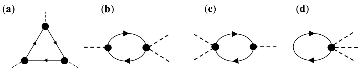
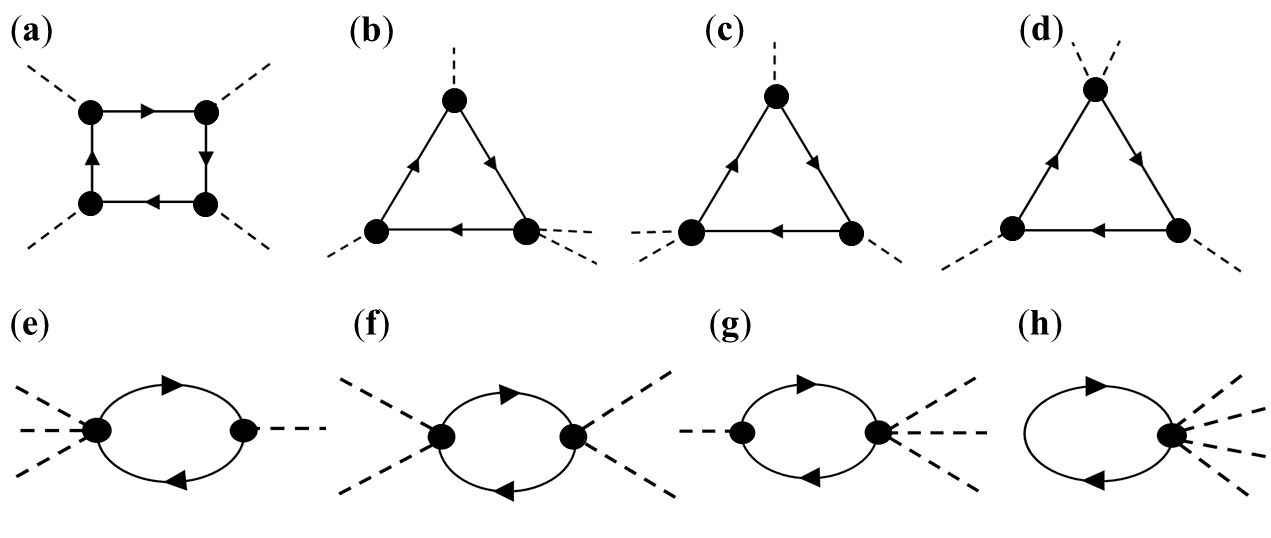
where and respectively stand for the second-and third-order spin-resolved susceptibility tensor elements in the two-dimensional x-y coordinate. In addition, and stand for the field elements at two colors with frequency and . We employ the diagrammatic perturbative approach, and the response functions are represented by the Feynman diagrams in Fig. 2 and 3. The solid lines are non-interacting fermionic propagators, while solid circles represent current vertices.
The second-order spin-resolved current given by the correlation of three paramagnetic current operators (or one-photon current coupling) as and can be diagrammatically depicted as in Fig. 2(a) which formally reads
| (6) |
where , is the energy difference between different bands with given spin index and refers to the difference between the Fermi function corresponding to distinct bands. Here is the Fermi-Dirac distribution function, is the chemical potential, and having as the Boltzmann constant, as an electron temperature. The one-photon coupling vertex is with being an eigen vector of the Hamiltonian. Note that stands for the intrinsic permutation symmetry and with the parameter . The diamagnetic contribution to the second-order response (Fig. 2(b)-(d)) is given by
| (7) |
Notice that the two-photon and three-photon current couplings are and , respectively.
Similarly, following the diagrammatic scheme in Fig. 3 (a), to written third-order spin response originating from the paramagnetic current operator is formally given by . In principle, there are seven distinct Feynman diagrams involving multi-photon current couplings Rostami et al. (2021). However, for our Hamiltonian model, only four additional diagrams can contribute, as depicted in Fig. 3(b,c,d,f), which can be written in terms of the following correlation functions , , and . We provide the explicit form of the third-order response in Appendix A for brevity.
II.1 Nonlinear spin Hall current
The -order nonlinear response functions to external fields are dictated by the susceptibility tensor components . The tensor components are restricted by space inversion, time reversal, and rotational and mirror symmetries of the crystalline quantum material. Specifically, for a system having mirror symmetry along the plane perpendicular to an arbitrary spatial axis and the spin polarization direction, the susceptibility tensor components with an odd number of ‘’ spatial indices do not contribute to the charge current. This arises due to the cancellation of the up and down spin components as . But, these tensor components contribute to the spin response function .
In the time-reversal symmetric WTe2 with broken inversion symmetry due to vertical gate potential, the mirror symmetry with respect to -axis, i.e., reduces non-vanishing tensor elements to four and eight for the second-order and third-order responses respectively. These second-order components are . For the third-order response, the non-vanishing tensor elements are the following
| (8) |
To demonstrate the polarization dependence, we decompose the nonlinear spin Hall current in the longitudinal and transverse basis as . Here, the unit vectors are orthogonal .
Accordingly, the longitudinal (parallel) and transverse (perpendicular) components of the spin current can be formulated using the relation and respectively. In this study, we focus on the transverse (Hall) components of the nonlinear rectified spin current due to single-color driving field and two-color light field where , with being the polarization angle, is the linear polarization unit vector. The corresponding light-induced single-color and two-color nonlinear spin-current are given by and respectively. Symmetry-based argument (as discussed earlier) leads to the following polarisation dependence of the transverse component of the nonlinear spin currents:
| (9) |
and the two-color spin Hall current is given by
| (10) |
where , , and
| (11) |
The derivation of the nonlinear spin currents is provided in Appendix B.
Further, is the phase difference between the single- and second-harmonic frequency beams. Here, we get two sets of terms that are proportional to and contribute to the third-order rectified spin Hall current depending on the choice of phase difference. It has been found that for the linearly polarized beams with , the nonlinear Hall current Eq. (10) yields maximum value as discussed in Ref. Rioux et al. (2011) for the case of graphene. In this study, we consider zero phase difference .
The following section presents numerical results in gated single-layer 1T′-WTe2 for the second and third-order spin susceptibilities versus laser frequency and the gate potential . Afterward, we analyze the anisotropic polarisation dependence of the nonlinear spin Hall susceptibilities.

III Numerical Results and Discussion
We provide numerical results for second and third-order spin Hall current induced by monochromatic and two-color laser excitations, respectively.
There are no second-order spin current () in the Hall measurement geometry along -direction with the field along -direction due to the cancellation of the current induced by up and down spins, but the second-order Hall charge current will remain finite. Unlike the second-order current, the third-order spin Hall current follows different symmetry properties, thus can be obtained in both and Hall measurement geometries. Specifically, the third-order spin Hall effect can be observed in both inversion symmetric and time-reversal symmetric materials. Here, we discuss the two Hall components of susceptibility , and , subjected to the mirror symmetry possessed by 1T′-WTe2, to the linearly polarized two-color optical beam of light. The two beams at frequency and interfere, resulting in the third-order rectified spin current.
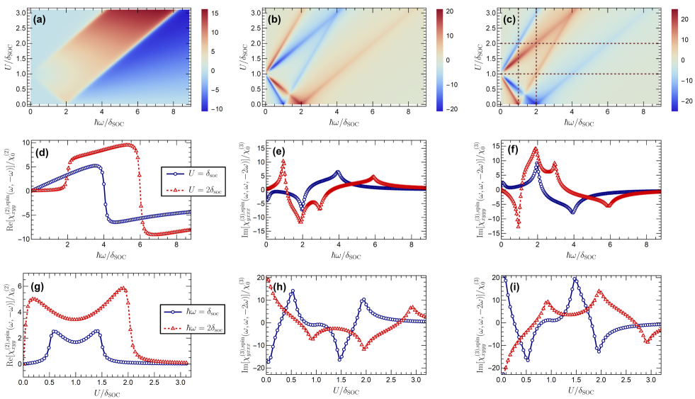
In Fig. 4 (a)-(c), we demonstrate the density plot for the second-and third-order spin Hall susceptibility tensor components , and for 1T′-WTe2 having spin texture in the momentum space, as a function of and , where is the spin-orbit coupling gap. Here, we mainly focus on the rectified (dc) spin current with single-color and two-color laser beams, contributed by the real part of the second-order and imaginary part of the third-order response functions, respectively.
We observe that the second-order spin Hall susceptibility component in response to the electric field along direction gives interband resonances at an incident energy , with being the band gap at and , as indicated by the dark red and dark blue colors in Fig. 4(a). However, resonances’ strength and position change with the out-of-plane gate potential, thus shifting in different frequency regimes.
The resulting feature is intriguing because of the band closing and reopening around the Dirac points at valleys and due to the gate potential . Furthermore, the spin current generation occurs due to the imbalance of carrier excitation at different valleys. Since spin-up and spin-down currents are equal in magnitude and flow in opposite directions, the charge Hall current vanishes and we obtain a pure second-order spin Hall current by irradiating the linearly polarized single-color beam of light.
One of the most striking results of this study is the in-gap light-induced nonlinear spin current when . Unlike usual shift and injection current mechanisms which are related to the imaginary part of , the in-gap current is given by the real part . In the clean limit, the imaginary part leads to a delta function implying that we can induce a current after absorbing the photon and generating a photo-excited carrier. However, the in-gap current is related to the principal value of and thus can be finite even without generating a photo-excited carrier density. This mechanism has been discussed for the second-order charge current in time-reversal symmetry breaking systems Kaplan et al. (2020); Gao et al. (2021), and its thermodynamics ground is discussed in details Shi et al. (2022). For the case of zero phase difference, the two-color rectified spin current is given by the real part of the third-order conductivity (see Appendix B)
| (12) |
The real part of two-color third-order conductivity contains principle value terms that can technically explain the emergence of in-gap current. Here, we show that one can generate third-order in-gap spin current in a time-reversal symmetric system. However, there is no in-gap effect in the second-order spin response due to the cancellation of the effect for spin-up and spin-down components.
To illustrate features with more detail, we plot the cross-section curves at different values of the scaled back-gate potential and the incident photon energy . For , the inversion symmetry of the system remains intact, which results in the vanishing second-order response consistent with the symmetry argument. For finite but small , the inversion symmetry breaks down that leads to finite .
As seen in Fig. 4(d), the effective band gap vanishes, and the bottom of the conduction and top of the valence bands touch each other at point when and therefore optical response reveals the gapless nature of the system that is finite even at the tiny value of the light frequency. By further increasing the frequency, we see a step-like feature in the second order response at . We have generated the same curve for the case of where the effective gaps at different valleys are and . This leads to the resonant jumps at and .
In Fig. 4(e)-(f), we find the emergence of resonant peaks in the third-order response due to the two-photon and one-photon absorption processes which correspond to and , respectively. Among these, the two peaks associated with a larger effective gap show similar behavior, such as resonances for different back-gate potentials. However, the other two associated with reveal the different feature that is the presence and absence of the resonance peak at and .
We have constructed vertical cross-section plots to investigate the behavior of nonlinear spin susceptibilities concerning fixed values of photon energy and varying values of . The second-order and third-order effects are depicted in Fig. 4(g) and Fig. 4(h)-(i), respectively. Contrary to the second-order case, the third-order response remains finite at . Furthermore, we observe a strong and non-monotonic dependence of the nonlinear spin current on the back-gate potential . This behavior implies that small changes in the back-gate potential can induce significant changes in the resulting nonlinear spin response, which could have important implications for the design and optimization of spin-based devices.
Further, we present the numerical results for the polarisation dependence of the spin transverse currents for a fixed value of in polar plots in Fig. 5. The polarization dependence of nonlinear spin current highly depends on the crystalline symmetry and orientation of the monolayer WTe2. The anisotropic behavior of the second-order spin Hall current that follows . The third-order spin current is proportional to the imaginary part of components for zero phase difference between two color laser pulses. The anisotropic polarization dependence of third-order spin current is more complex due to the competing behavior of different tensor components of the susceptibility multiplied by , , and .
Finally, we provide the numerical estimation of the spin Hall photocurrents at a particular incident energy and using the microscopic parameter obtained from DFT calculations and experiments Tang et al. (2017); Xu et al. (2018); Garcia et al. (2020b). At meV, which is twice the spin-orbit coupling gap meV, the out-of-plane gate potential meV, and the electric field of the order of V/m, the magnitude of the second and third-order rectified spin Hall conductivity comes out to be of the order of and respectively, where is the unit of spin conductivity. Here, the back-gate potential is obtained using the relation and setting vertical field V/nm, dielectric constant , and the separation between the top and bottom contacts nm aturia et al. (2018); Shahnazaryan et al. (2019). Compared to the linear dc spin conductivity, the presented rectified nonlinear spin Hall conductivity estimation is feasible to measure experimentally.
IV Conclusion
Our study focuses on the investigation of the rectified nonlinear spin Hall current in the 1T′-WTe2 material, utilizing both single-color and two-color laser beams. We have conducted an extensive analysis on the effects of the displacement field, light intensity, and polarization direction on the nonlinear spin Hall current to gain a comprehensive understanding of this phenomenon. Our findings indicate that the nonlinear response exhibits interband resonances arising from one-photon and two-photon absorption processes. It is worth noting that the two-color rectified response was found to be significantly stronger in magnitude than the single-color response when the displacement field was twice the spin-orbit coupling gap. Remarkably, we have also discovered the presence of an in-gap third-order spin current that is finite even when the light frequency is within the electronic bandgap. This discovery has significant implications for future research and technological advancements. Our study provides valuable insights into the intrinsic nonlinear spin hall effect in the 1T′-WTe2 material and offers a path toward designing advanced optoelectronic devices capable of operating in nonlinear regimes for spintronics applications.
Acknowledgment
This work was supported by Nordita and the Swedish Research Council (VR Starting Grant No. 2018-04252). Nordita is partially supported by Nordforsk. PB acknowledges the computational facilities provided by SRM-AP.
References
- Keimer and Moore (2017) B. Keimer and J. E. Moore, “The physics of quantum materials,” Nature Physics 13, 1045 (2017).
- Giustino et al. (2020) Feliciano Giustino, Jin Hong Lee, Felix Trier, Manuel Bibes, Stephen M Winter, Roser Valentí, Young-Woo Son, Louis Taillefer, Christoph Heil, Adriana I Figueroa, Bernard Plaçais, QuanSheng Wu, Oleg V Yazyev, Erik P A M Bakkers, Jesper Nygård, Pol Forn-Díaz, Silvano De Franceschi, J W McIver, L E F Foa Torres, Tony Low, Anshuman Kumar, Regina Galceran, Sergio O Valenzuela, Marius V Costache, Aurélien Manchon, Eun-Ah Kim, Gabriel R Schleder, Adalberto Fazzio, and Stephan Roche, “The 2021 quantum materials roadmap,” Journal of Physics: Materials 3, 042006 (2020).
- Sodemann and Fu (2015) Inti Sodemann and Liang Fu, “Quantum nonlinear hall effect induced by berry curvature dipole in time-reversal invariant materials,” Phys. Rev. Lett. 115, 216806 (2015).
- Morimoto and Nagaosa (2016) Takahiro Morimoto and Naoto Nagaosa, “Topological nature of nonlinear optical effects in solids,” Science Advances 2, e1501524 (2016).
- de Juan et al. (2017) Fernando de Juan, Adolfo G. Grushin, Takahiro Morimoto, and Joel E Moore, “Quantized circular photogalvanic effect in weyl semimetals,” Nature Communications 8, 15995 (2017).
- Rostami and Polini (2018) Habib Rostami and Marco Polini, “Nonlinear anomalous photocurrents in weyl semimetals,” Phys. Rev. B 97, 195151 (2018).
- Wang and Qian (2019) Hua Wang and Xiaofeng Qian, “Ferroicity-driven nonlinear photocurrent switching in time-reversal invariant ferroic materials,” Science Advances 5, eaav9743 (2019).
- Mueller and Malic (2018) Thomas Mueller and Ermin Malic, “Exciton physics and device application of two-dimensional transition metal dichalcogenide semiconductors,” npj 2D Materials and Applications 2, 29 (2018).
- Soavi et al. (2018) Giancarlo Soavi, Gang Wang, Habib Rostami, David G. Purdie, Domenico De Fazio, Teng Ma, Birong Luo, Junjia Wang, Anna K. Ott, Duhee Yoon, Sean A. Bourelle, Jakob E. Muench, Ilya Goykhman, Stefano Dal Conte, Michele Celebrano, Andrea Tomadin, Marco Polini, Giulio Cerullo, and Andrea C. Ferrari, “Broadband, electrically tunable third-harmonic generation in graphene,” Nature Nanotechnology 13, 583–588 (2018).
- Principi et al. (2019) Alessandro Principi, Denis Bandurin, Habib Rostami, and Marco Polini, “Pseudo-euler equations from nonlinear optics: Plasmon-assisted photodetection beyond hydrodynamics,” Phys. Rev. B 99, 075410 (2019).
- Bhalla et al. (2020) Pankaj Bhalla, Allan H. MacDonald, and Dimitrie Culcer, “Resonant photovoltaic effect in doped magnetic semiconductors,” Phys. Rev. Lett. 124, 087402 (2020).
- Wang et al. (2021) Yadong Wang, Fadil Iyikanat, Habib Rostami, Xueyin Bai, Xuerong Hu, Susobhan Das, Yunyun Dai, Luojun Du, Yi Zhang, Shisheng Li, Harri Lipsanen, F. Javier García de Abajo, and Zhipei Sun, “Probing electronic states in monolayer semiconductors through static and transient third-harmonic spectroscopies,” Advanced Materials 34, 2107104 (2021).
- Klimmer et al. (2021) Sebastian Klimmer, Omid Ghaebi, Ziyang Gan, Antony George, Andrey Turchanin, Giulio Cerullo, and Giancarlo Soavi, “All-optical polarization and amplitude modulation of second-harmonic generation in atomically thin semiconductors,” Nature Photonics 15, 837 (2021).
- Bhalla (2021) Pankaj Bhalla, “Intrinsic contribution to nonlinear thermoelectric effects in topological insulators,” Phys. Rev. B 103, 115304 (2021).
- Sinha et al. (2022) Subhajit Sinha, Pratap Chandra Adak, Atasi Chakraborty, Kamal Das, Koyendrila Debnath, L. D. Varma Sangani, Kenji Watanabe, Takashi Taniguchi, Umesh V. Waghmare, Amit Agarwal, and Mandar M. Deshmukh, “Berry curvature dipole senses topological transition in a moire superlattice,” Nature Physics 18, 765 (2022).
- Bhalla and Rostami (2022) Pankaj Bhalla and Habib Rostami, “Second harmonic helicity and faraday rotation in gated single-layer 1T’-WTe2,” Phys. Rev. B 105, 235132 (2022).
- Chakraborty et al. (2022) Atasi Chakraborty, Kamal Das, Subhajit Sinha, Pratap Chandra Adak, Mandar M Deshmukh, and Amit Agarwal, “Nonlinear anomalous hall effects probe topological phase-transitions in twisted double bilayer graphene,” 2D Materials 9, 045020 (2022).
- Bhalla et al. (2022a) Pankaj Bhalla, Kamal Das, Dimitrie Culcer, and Amit Agarwal, “Resonant second-harmonic generation as a probe of quantum geometry,” Phys. Rev. Lett. 129, 227401 (2022a).
- Lahiri et al. (2022) Shibalik Lahiri, Kamal Das, Dimitrie Culcer, and Amit Agarwal, “Intrinsic nonlinear conductivity induced by the quantum metric dipole,” (2022), 10.48550/ARXIV.2207.02178.
- Bhalla et al. (2021) Pankaj Bhalla, Ming-Xun Deng, Rui-Qiang Wang, Lan Wang, and Dimitrie Culcer, “Nonlinear ballistic response of quantum spin hall edge states,” Phys. Rev. Lett. 127, 206801 (2021).
- Zeng et al. (2022) Chuanchang Zeng, Snehasish Nandy, and Sumanta Tewari, “Chiral anomaly induced nonlinear nernst and thermal hall effects in weyl semimetals,” Phys. Rev. B 105, 125131 (2022).
- Bhalla et al. (2022b) Pankaj Bhalla, Giovanni Vignale, and Habib Rostami, “Pseudogauge field driven acoustoelectric current in two-dimensional hexagonal dirac materials,” Phys. Rev. B 105, 125407 (2022b).
- Bhalla et al. (2022c) Pankaj Bhalla, Kamal Das, Amit Agarwal, and Dimitrie Culcer, “Quantum kinetic theory of nonlinear optical currents: Finite fermi surface and fermi sea contributions,” (2022c), 10.48550/ARXIV.2212.10330.
- Ikeda et al. (2023) Yuya Ikeda, Sota Kitamura, and Takahiro Morimoto, “Photocurrent induced by a bicircular light drive in centrosymmetric systems,” (2023), 10.48550/ARXIV.2303.01796.
- Shvetsov et al. (2019) O. O. Shvetsov, V. D. Esin, A. V. Timonina, N. N. Kolesnikov, and E. V. Deviatov, “Nonlinear hall effect in three-dimensional weyl and dirac semimetals,” JETP Letters 109, 715 (2019).
- Tiwari et al. (2021) Archana Tiwari, Fangchu Chen, Shazhou Zhong, Elizabeth Drueke, Jahyun Koo, Austin Kaczmarek, Cong Xiao, Jingjing Gao, Xuan Luo, Qian Niu, Yuping Sun, Binghai Yan, Liuyan Zhao, and Adam W. Tsen, “Giant c-axis nonlinear anomalous hall effect in Td-MoTe2 and WTe2,” Nature Communications 12, 2049 (2021).
- Ma et al. (2019) Qiong Ma, Su-Yang Xu, Huitao Shen, David MacNeill, Valla Fatemi, Tay-Rong Chang, Andrés M. Mier Valdivia, Sanfeng Wu, Zongzheng Du, Chuang-Han Hsu, Shiang Fang, Quinn D. Gibson, Kenji Watanabe, Takashi Taniguchi, Robert J. Cava, Efthimios Kaxiras, Hai-Zhou Lu, Hsin Lin, Liang Fu, Nuh Gedik, and Pablo Jarillo-Herrero, “Observation of the nonlinear hall effect under time-reversal-symmetric conditions,” Nature 565, 337 (2019).
- Kang et al. (2019) Kaifei Kang, Tingxin Li, Egon Sohn, Jie Shan, and Kin Fai Mak, “Nonlinear anomalous hall effect in few-layer WTe2,” Nature Materials 18, 324 (2019).
- Sun and Xie (2005) Qing-feng Sun and X. C. Xie, “Definition of the spin current: The angular spin current and its physical consequences,” Phys. Rev. B 72, 245305 (2005).
- Kane and Mele (2005) C. L. Kane and E. J. Mele, “Quantum spin hall effect in graphene,” Phys. Rev. Lett. 95, 226801 (2005).
- Bernevig et al. (2006) B. Andrei Bernevig, Taylor L. Hughes, and Shou-Cheng Zhang, “Quantum spin hall effect and topological phase transition in hgte quantum wells,” Science 314, 1757 (2006).
- Bernevig and Zhang (2006) B. Andrei Bernevig and Shou-Cheng Zhang, “Quantum spin hall effect,” Phys. Rev. Lett. 96, 106802 (2006).
- Qi et al. (2006) Xiao-Liang Qi, Yong-Shi Wu, and Shou-Cheng Zhang, “Topological quantization of the spin hall effect in two-dimensional paramagnetic semiconductors,” Phys. Rev. B 74, 085308 (2006).
- Xu and Moore (2006) Cenke Xu and J. E. Moore, “Stability of the quantum spin hall effect: Effects of interactions, disorder, and topology,” Phys. Rev. B 73, 045322 (2006).
- Ishizuka and Sato (2022) Hiroaki Ishizuka and Masahiro Sato, “Large photogalvanic spin current by magnetic resonance in bilayer cr trihalides,” Phys. Rev. Lett. 129, 107201 (2022).
- Sakimura et al. (2014) Hiroto Sakimura, Takaharu Tashiro, and Kazuya Ando, “Nonlinear spin-current enhancement enabled by spin-damping tuning,” Nature Communications 5, 5730 (2014).
- Nair et al. (2020) Jayakrishnan M. P. Nair, Zhedong Zhang, Marlan O. Scully, and Girish S. Agarwal, “Nonlinear spin currents,” Phys. Rev. B 102, 104415 (2020).
- Hamamoto et al. (2017a) Keita Hamamoto, Motohiko Ezawa, Kun Woo Kim, Takahiro Morimoto, and Naoto Nagaosa, “Nonlinear spin current generation in noncentrosymmetric spin-orbit coupled systems,” Phys. Rev. B 95, 224430 (2017a).
- Bhat et al. (2005) R. D. R Bhat, F. Nastos, Ali Najmaie, and J. E. Sipe, “Pure spin current from one-photon absorption of linearly polarized light in noncentrosymmetric semiconductors,” Phys. Rev. Lett. 94, 096603 (2005).
- Lihm and Park (2022) Jae-Mo Lihm and Cheol-Hwan Park, “Comprehensive theory of second-order spin photocurrents,” Phys. Rev. B 105, 045201 (2022).
- Du et al. (2021) Z. Z. Du, Hai-Zhou Lu, and X. C. Xie, “Nonlinear hall effects,” Nature Reviews Physics 3, 744–752 (2021).
- Garcia et al. (2020a) Jose H. Garcia, Marc Vila, Chuang-Han Hsu, Xavier Waintal, Vitor M. Pereira, and Stephan Roche, “Canted persistent spin texture and quantum spin hall effect in ,” Phys. Rev. Lett. 125, 256603 (2020a).
- Zhou and Shen (2007) Bin Zhou and Shun-Qing Shen, “Deduction of pure spin current from the linear and circular spin photogalvanic effect in semiconductor quantum wells,” Phys. Rev. B 75, 045339 (2007).
- Ivchenko and Tarasenko (2008) E L Ivchenko and S A Tarasenko, “Pure spin photocurrents,” Semiconductor Science and Technology 23, 114007 (2008).
- Tarasenko and Ivchenko (2005) S. A. Tarasenko and E. L. Ivchenko, “Pure spin photocurrents in low-dimensional structures,” Journal of Experimental and Theoretical Physics Letters 81, 5 (2005).
- Zhao et al. (2005) Hui Zhao, Xinyu Pan, Arthur L. Smirl, R. D. R. Bhat, Ali Najmaie, J. E. Sipe, and H. M. van Driel, “Injection of ballistic pure spin currents in semiconductors by a single-color linearly polarized beam,” Phys. Rev. B 72, 201302 (2005).
- Wang et al. (2010) Jing Wang, Bang-Fen Zhu, and Ren-Bao Liu, “Second-order nonlinear optical effects of spin currents,” Phys. Rev. Lett. 104, 256601 (2010).
- Hamamoto et al. (2017b) Keita Hamamoto, Motohiko Ezawa, Kun Woo Kim, Takahiro Morimoto, and Naoto Nagaosa, “Nonlinear spin current generation in noncentrosymmetric spin-orbit coupled systems,” Phys. Rev. B 95, 224430 (2017b).
- Du et al. (2018) Z. Z. Du, C. M. Wang, Hai-Zhou Lu, and X. C. Xie, “Band signatures for strong nonlinear hall effect in bilayer ,” Phys. Rev. Lett. 121, 266601 (2018).
- Xu et al. (2018) Su-Yang Xu, Qiong Ma, Huitao Shen, Valla Fatemi, Sanfeng Wu, Tay-Rong Chang, Guoqing Chang, Andrés M. Mier Valdivia, Ching-Kit Chan, Quinn D. Gibson, Jiadong Zhou, Zheng Liu, Kenji Watanabe, Takashi Taniguchi, Hsin Lin, Robert J. Cava, Liang Fu, Nuh Gedik, and Pablo Jarillo-Herrero, “Electrically switchable berry curvature dipole in the monolayer topological insulator WTe2,” Nature Physics 14, 900 (2018).
- Qian et al. (2014) Xiaofeng Qian, Junwei Liu, Liang Fu, and Ju Li, “Quantum spin hall effect in two-dimensional transition metal dichalcogenides,” Science 346, 1344 (2014).
- Fregoso (2019) Benjamin M. Fregoso, “Bulk photovoltaic effects in the presence of a static electric field,” Phys. Rev. B 100, 064301 (2019).
- Fregoso et al. (2018) Benjamin M. Fregoso, Rodrigo A. Muniz, and J. E. Sipe, “Jerk current: A novel bulk photovoltaic effect,” Phys. Rev. Lett. 121, 176604 (2018).
- Ahn et al. (2022) Junyeong Ahn, Guang-Yu Guo, Naoto Nagaosa, and Ashvin Vishwanath, “Riemannian geometry of resonant optical responses,” Nature Physics 18, 290–295 (2022).
- Manykin and Afanasev (1967) E.A. Manykin and A.M. Afanasev, “On one possibility of making a medium transparent by multiquantum resonance,” JETP 25, 828 (1967).
- Bhat and Sipe (2000) R. D. R. Bhat and J. E. Sipe, “Optically injected spin currents in semiconductors,” Phys. Rev. Lett. 85, 5432–5435 (2000).
- Rioux et al. (2011) J. Rioux, Guido Burkard, and J. E. Sipe, “Current injection by coherent one- and two-photon excitation in graphene and its bilayer,” Phys. Rev. B 83, 195406 (2011).
- Khurgin (1995) J. B. Khurgin, “Generation of the teraherz radiation using in semiconductor,” Journal of Nonlinear Optical Physics & Materials 04, 163–189 (1995).
- Totero Gongora et al. (2020) J. S. Totero Gongora, L. Peters, J. Tunesi, V. Cecconi, M. Clerici, A. Pasquazi, and M. Peccianti, “All-optical two-color terahertz emission from quasi-2d nonlinear surfaces,” Phys. Rev. Lett. 125, 263901 (2020).
- Cheng et al. (2014) J L Cheng, N Vermeulen, and J E Sipe, “Third order optical nonlinearity of graphene,” New Journal of Physics 16, 053014 (2014).
- Cheng et al. (2015) J. L. Cheng, N. Vermeulen, and J. E. Sipe, “Third-order nonlinearity of graphene: Effects of phenomenological relaxation and finite temperature,” Phys. Rev. B 91, 235320 (2015).
- Atanasov et al. (1996) R. Atanasov, A. Haché, J. L. P. Hughes, H. M. van Driel, and J. E. Sipe, “Coherent control of photocurrent generation in bulk semiconductors,” Phys. Rev. Lett. 76, 1703–1706 (1996).
- Haché et al. (1997) A. Haché, Y. Kostoulas, R. Atanasov, J. L. P. Hughes, J. E. Sipe, and H. M. van Driel, “Observation of coherently controlled photocurrent in unbiased, bulk gaas,” Phys. Rev. Lett. 78, 306–309 (1997).
- Kaplan et al. (2020) Daniel Kaplan, Tobias Holder, and Binghai Yan, “Nonvanishing subgap photocurrent as a probe of lifetime effects,” Phys. Rev. Lett. 125, 227401 (2020).
- Gao et al. (2021) Lingyuan Gao, Zachariah Addison, E. J. Mele, and Andrew M. Rappe, “Intrinsic fermi-surface contribution to the bulk photovoltaic effect,” Phys. Rev. Research 3, L042032 (2021).
- Garcia et al. (2020b) Jose H. Garcia, Marc Vila, Chuang-Han Hsu, Xavier Waintal, Vitor M. Pereira, and Stephan Roche, “Canted persistent spin texture and quantum spin hall effect in ,” Phys. Rev. Lett. 125, 256603 (2020b).
- Tang et al. (2017) Shujie Tang, Chaofan Zhang, Dillon Wong, Zahra Pedramrazi, Hsin-Zon Tsai, Chunjing Jia, Brian Moritz, Martin Claassen, Hyejin Ryu, Salman Kahn, Juan Jiang, Hao Yan, Makoto Hashimoto, Donghui Lu, Robert G. Moore, Chan-Cuk Hwang, Choongyu Hwang, Zahid Hussain, Yulin Chen, Miguel M. Ugeda, Zhi Liu, Xiaoming Xie, Thomas P. Devereaux, Michael F. Crommie, Sung-Kwan Mo, and Zhi-Xun Shen, “Quantum spin hall state in monolayer 1T’-WTe2,” Nature Physics 13, 683 (2017).
- Rostami et al. (2021) Habib Rostami, Mikhail I. Katsnelson, Giovanni Vignale, and Marco Polini, “Gauge invariance and ward identities in nonlinear response theory,” Annals of Physics 431, 168523 (2021).
- Shi et al. (2022) Li-kun Shi, Oles Matsyshyn, Justin CW Song, and Inti Sodemann Villadiego, “The berry dipole photovoltaic demon and the thermodynamics of photo-current generation within the optical gap of metals,” arXiv:2207.03496 (2022).
- aturia et al. (2018) Akash aturia, Maarten L. Van de Put, and William G. Vandenberghe, “Dielectric properties of hexagonal boron nitride and transition metal dichalcogenides: from monolayer to bulk,” npj 2D Materials and Applications 2, 6 (2018).
- Shahnazaryan et al. (2019) V. Shahnazaryan, O. Kyriienko, and H. Rostami, “Exciton routing in the heterostructure of a transition metal dichalcogenide monolayer on a paraelectric substrate,” Phys. Rev. B 100, 165303 (2019).
- Säynätjoki et al. (2017) Antti Säynätjoki, Lasse Karvonen, Habib Rostami, Anton Autere, Soroush Mehravar, Antonio Lombardo, Robert A. Norwood, Tawfique Hasan, Nasser Peyghambarian, Harri Lipsanen, Khanh Kieu, Andrea C. Ferrari, Marco Polini, and Zhipei Sun, “Ultra-strong nonlinear optical processes and trigonal warping in mos2 layers,” Nature Communications 8, 893 (2017).
Appendix A Third-order susceptibility expression
In a similar spirit of the second-order response, the paramagnetic contribution to the third-order response corresponding to the Feynman diagram Fig. 3(a) is given by Säynätjoki et al. (2017); Ahn et al. (2022)
| (13) |
and the diamagnetic part of the third-order susceptibility associated with Figs. 3(b)-(h) is given by Säynätjoki et al. (2017); Rostami et al. (2021)
| (14) |
Appendix B Nonlinear rectified currents
B.1 Second-order rectified current
The second-order rectified current is obtained by setting . In response to a time-dependent external electric field , the current can be expressed as follows
| (15) |
Here, the conductivity is . Further, on considering the spatial indices we get
| (16) | ||||
Note that . Expressing the conductivity in real and imaginary parts as and using the relation , we obtain
| (17) |
B.2 Third-order rectified current
The third-order rectified current is obtained by setting . In response to a time-dependent external electric field , the current can be expressed as follows
| (18) |
Here, the conductivity is . Further, on considering the spatial indices we get
| (19) |
Considering real-valued field amplitudes, we obtain
| (20) |
Writing the conductivity in real and imaginary parts as and using the relation , we obtain
| (21) |
B.3 Transverse component of the nonlinear spin currents
For the single-color driving field , the transverse nonlinear rectified current is given by
| (22) |
where the unit vector and is the linear polarization unit vector having an angle of polarization. Using this property, the transverse current becomes
| (23) |
Using Eq. (17) and expressing and considering the symmetry-permitted components of the second-order response in gated single-layer WTe2, we obtain
| (24) |
On further simplifications, the rectified second-order current yields
| (25) |
This derivation leads to Eq. (9) in the main text. Similarly, for the two-color light field the third-order rectified transverse current following Eq. (21) gives
| (26) | |||
| (27) |
On substituting the field, the above equation reduces to
| (28) |
| (29) |
where the quantities , , , and . This derives the Eq. (10) of the main text.