Abstract

Item response theory (IRT) is the study of how people make probabilistic decisions, with diverse applications in education testing, recommendation systems, among others. The Rasch model of binary response data, one of the most fundamental models in IRT, remains an active area of research with important practical significance. Recently, Nguyen and Zhang (2022) proposed a new spectral estimation algorithm that is efficient and accurate. In this work, we extend their results in two important ways.

Firstly, we obtain a refined entrywise error bound for the spectral algorithm, complementing the ‘average error’ $\ell_{2}$ bound in their work. Notably, under mild sampling conditions, the spectral algorithm achieves the minimax optimal error bound (modulo a log factor). Building on the refined analysis, we also show that the spectral algorithm enjoys optimal sample complexity for top-$K$ recovery (e.g., identifying the best $K$ items from approval/disapproval response data), explaining the empirical findings in the previous work.

Our second contribution addresses an important but understudied topic in IRT: privacy. Despite the human-centric applications of IRT, there has not been any proposed privacy-preserving mechanism in the literature. We develop a private extension of the spectral algorithm, leveraging its unique Markov chain formulation and the discrete Gaussian mechanism (Canonne et al., 2020). Experiments show that our approach is significantly more accurate than the baselines in the low-to-moderate privacy regime.

1 INTRODUCTION

Item response theory (IRT) was originally developed within the psychometric community in the early 60s (Rasch,, 1960; Van der Linden and Hambleton,, 1997) as a tool to model patients’ responses to psychological tests. Since its conception, item response theory has been applied to diverse settings including education testing (Lord,, 2012), crowdsourcing (Whitehill et al.,, 2009), recommendation systems (Chen et al.,, 2005), finance (Schellhorn and Sharma,, 2013), marketing (Brzezińska et al.,, 2016) and more recently the evaluation of machine learning algorithms (Moraes et al.,, 2020; Chen and Ahn,, 2020; Martínez-Plumed et al.,, 2019).

One of the most fundamental models in IRT is the Rasch model (Rasch,, 1960). It assumes that the binary response $X_{li}\in\{0,1\}$ of person $l$ with latent characteristic $\theta^{*}_{l}\in\mathbb{R}$ to item $i$ with latent parameter $\beta^{*}_{i}\in\mathbb{R}$ is given as follows.

$$\mathbb{P}(X_{li}=1)=\frac{1}{1+\mathrm{exp}\left(-(\theta^{*}_{l}-\beta^{*}_{i})\right)}\,.$$ (1)

As an example in education testing, $\theta^{*}_{l}$ corresponds to the ability of student $l$ and $\beta^{*}_{i}$ the difficulty of problem $i$. The random response variable $X_{li}$ is whether the student correctly solves the problem. Recently, Nguyen and Zhang, (2022) proposed a new spectral algorithm for one-sided parameter estimation under the Rasch model (i.e., estimate $\beta^{*}$). Experimentally, the spectral algorithm is significantly faster than its competitors while being comparatively accurate. As the spectral algorithm is entirely new, we identify two important open directions from the previous work.

Entrywise Error Guarantee. The guarantee in Nguyen and Zhang, (2022) is an $\ell_{2}$ error bound for parameter estimation (cf., Theorem 3.3), which can be roughly considered the average estimation error. In certain domains, we might desire a small entrywise error guarantee. For example, consider a conference reviewing system where reviewers vote to reject or accept papers. We would like to accurately identify the top papers from reject/accept data. One approach is to estimate the quality parameters of the papers and accept $K$ papers with the higest parameter values. The $\ell_{2}$ error does not indicate how the estimation error distributes among the papers. The average error may still be low if all the error is concentrated in a single estimate. Really good papers could get rejected or subpar papers get accepted. On the other hand, a small entrywise parameter estimation error ensures that the quality for each paper is accurately measured.

Privacy. The study of privacy-preserving mechanisms in IRT is understudied. This is quite concerning because many item response theory models and algorithms are deployed on human response data containing sensitive information (e.g., a student passing a test, a voter supporting a legislation). One may consider the binary nature of the response data and propose randomized response (Warner,, 1965) as a natural solution. However, as we will show in our experiments, even when the number of responses per person is moderate $m\approx 10$, the amount of noise that randomized response needs to inject to ensure sufficient privacy is too large for any downstream algorithm to obtain accurate parameter estimates. On the other hand, analyzing the sensitivity (cf. Definition 3.1 in Dwork et al., (2014)) of the algorithms used in the IRT literature including optimization based algorithms (Andersen,, 1973; Fischer,, 1981; Haberman,, 1977; Hambleton et al.,, 1991) is substantially more difficult. This might explain the seeming lack of progress towards developing a private algorithm in IRT.

Our Contributions. In this work, we make progress in both of the above open directions.

• In section 3, we obtain refined entrywise analysis of the spectral algorithm, coupled with a matching lower bound, showing that under mild sampling conditions, the spectral algorithm achieves optimal entrywise error guarantee (up to a log factor). As a result of this optimality, we also show that the spectral algorithm can accurately identify all of the top $K$ items using only a constant factor more than the information theoretically minimal sample size.

• In Section 4, we propose a privacy-preserving mechanism that is designed with the discrete nature of human response data in mind. We take advantage of the Markov chain formulation underlying the spectral algorithm and the discrete Gaussian mechanism to develop a conceptually simple yet performant private algorithm. The algorithm provides strong and controllable privacy guarantee and outperforms other approaches, especially in the low-to-moderate privacy regime.

2 PROBLEM DESCRIPTION & THE SPECTRAL ALGORITHM

We follow the notations of Nguyen and Zhang, (2022). Consider a universe with $n$ people and $m$ items. Each person $l$ has parameter $\theta^{*}_{l}\in\mathbb{R}$ and each item $i$ has parameter $\beta^{*}_{i}\in\mathbb{R}$. To overcome a fundamental identifiability issue associated with parameter translation, we assume a normalization constraint on the item parameters ${\beta^{*}}^{\top}\mathbf{1}_{m}=0$. We also assume that $\beta^{*}_{i}\in[\beta^{*}_{\min},\beta^{*}_{\max}]\,\forall i\in[m]$ for some constants $\beta^{*}_{\min}$, $\beta^{*}_{\max}$. Similarly, we assume that $\theta^{*}_{l}\in[\theta^{*}_{\min},\theta^{*}_{\max}]$ for some constants $\theta^{*}_{\min},\theta^{*}_{\max}$. Let $A\in\{0,1\}^{n\times m}$ denote the assignment matrix where $A_{li}=1$ if person $l$ responds to item $i$ and $0$ indicates missing data. The observed data is $X\in\{0,1,*\}^{n\times m}$ where $*$ denotes missing data. For entries where $A_{li}=1$, $X_{li}$ is independently distributed per Equation (1). Let us consider the uniform sampling model where $A_{li}=1$ with probability $p$ for some $p>0$.

The Spectral Algorithm. We summarize the original formulation of the spectral algorithm here. For more details on its implementation and analysis, we refer the reader to Nguyen and Zhang, (2022). For each item pair $i\neq j$, define the pairwise differential measurement as

$$Y_{ij}=\sum_{l=1}^{n}A_{li}A_{lj}X_{li}(1-X_{lj})\quad\forall i\neq j\in[m]\,.$$ (2)

Note that this is a discrete-valued quantity. Given the pairwise differential measurements, the algorithm constructs a Markov chain $\hat{M}\in[0,1]^{m\times m}$ whose transition probabilities are defined as follows:

$$\hat{M}_{ij}=\begin{cases}\frac{1}{d}Y_{ij}&\text{ if $i\neq j$}\\ 1-\sum_{k\neq i}\frac{1}{d}Y_{ik}&\text{ if $i=j$}\end{cases}\quad,$$ (3)

where $d$ is a sufficiently large normalization factor chosen so that the resulting pairwise transition probability matrix $\hat{M}$ does not contain any negative entries. Typically, $d=O(\max_{i\in[m]}\sum_{k\neq i}B_{ik})$ where $B_{ik}=\sum_{l=1}^{n}A_{li}A_{lk}$. The algorithm then computes the stationary distribution $\pi$ of $\hat{M}$ and recovers $\beta$ using a post-processing step. Algorithm 1 summarizes the spectral algorithm.

Algorithm 1 The Spectral Algorithm

Input: Binary response data $X\in\{0,1,*\}^{n\times m}$.
    Output: Item parameter estimate $(\beta_{i})_{i=1}^{m}$.

1:  Construct a Markov chain $\hat{M}$ per Equation (3).

2:  Compute the stationary distribution of $\hat{M}$: Initialize $\pi^{(0)}=[\frac{1}{m},\ldots,\frac{1}{m}].$ For $t=1,2,\ldots$ until convergence, compute 

$${\pi^{(t)}}^{\top}=\frac{{\pi^{(t-1)}}^{\top}\hat{M}}{\lVert{\pi^{(t-1)}}^{\top}\hat{M}\rVert_{1}}\,.$$

3:  Compute $z=(\pi/d)/\lVert\pi/d\rVert_{1}$ and $\bar{\beta}_{i}=\log z_{i}$ for $i\in[m]$. Return the normalized item parameters, i.e., $\beta=\bar{\beta}-\bar{\beta}^{\top}\mathbf{1}/m$.

3 FINE-GRAIN ANALYSIS OF THE SPECTRAL ALGORITHM

3.1 Entrywise Error Bound

In this section we provide refined entrywise error bound for the spectral algorithm. Recall the example with conference reviewing and that our practical motivation is to show that the estimation error incurred by the spectral algorithm ‘spreads out’ among the parameters. This is to prevent the case where the estimation error is concentrated on a few items.

Theorem 3.1.

Consider the uniform sampling model described in Section 2. There exist constants $C_{1},C_{2}$ such that if $np^{2}\geq C_{1}\log m$ and $mp\geq C_{2}\log n$ then the output of the spectral algorithm satisfies

$$\lVert\beta-\beta^{*}\rVert_{\infty}\leq\frac{C\sqrt{\log m}}{\sqrt{np}}$$

with probability at least $1-\mathcal{O}\left(m^{-10}\right)-\mathcal{O}\left(n^{-10}\right)$ where $C$ is an absolute constant.

The above theorem is a refinement of Theorem 3.3 in Nguyen and Zhang, (2022). In that paper, the authors show that the output of the spectral algorithm satisfies $\lVert\beta-\beta^{*}\rVert_{2}=\mathcal{O}\left(\frac{\sqrt{m}}{\sqrt{np}}\right)\,.$ Comparing the this $\ell_{2}$ bound with Theorem 3.1 reveals that the magnitude of the entrywise error is no more than $\mathcal{O}\left(\sqrt{\frac{\log m}{m}}\right)$ the size of the $\ell_{2}$ error. This shows that the cummulative error indeed distributes evenly among the parameters and no two error terms differ in magnitude by more than a $\log$ factor.

Readers who are familiar with the learning to rank literature might see the parallel between this result and that in the Bradley-Terry-Luce (BTL) model where a similar algorithm – spectral ranking – enjoys a favorable entrywise error guarantee. However, the results are only superficially familiar and are based on similar fundamental theorems of Markov chain perturbation. Our results for the entrywise error bound and top-$K$ recovery in the next section are not simple extensions of the known results in the BTL literature. Firstly, the sampling model considered here fundamentally differs from the Erdos-Reyni comparison graph sampling model considered in the BTL model analysis. Additionally, the construction of the spectral algorithm is also different from the spectral ranking algorithm. Specifically, the pairwise transition probabilities and the construction of the Markov chain in Algorithm 1 and the spectral ranking algorithm are different.

Besides the spectral algorithm, we are only aware of entryise error guarantee for joint maximum likelihood estimate (JMLE) (Andersen,, 1973; Haberman,, 1977), formally stated in Theorem 2 of Chen et al., (2021). However, it is well known that JMLE produces an inconsistent estimate of $\beta^{*}$ when $m$ is constant (Andersen,, 1973; Ghosh,, 1995). In the supplementary materials, we provide a complementary entrywise error bound for the spectral algorithm where we remove the assumption $mp=\Omega\left(\log n\right)$ from Theorem 3.1, showing that the spectral method always gives a consistent estimation of individual item parameters. On a practical note, the spectral algorithm has been shown to be similar in terms of accuracy but is significantly faster than JMLE (Nguyen and Zhang,, 2022).

3.2 Top-$K$ Recovery Guarantee

In this section, we analyze the performance of the spectral algorithm in terms of top-$K$ recovery, building on the entrywise error bound obtained earlier. Curiously, Nguyen and Zhang, (2022) show through experimental results that the spectral algorithm often outperforms the baseline IRT algorithms in terms of top-$K$ accuracy. In this section, we provide a theoretical justification for its strong performance by furnishing an upper bound on the sample complexity for top-$K$ recovery of the spectral algorithm. Under mild sampling conditions, this upper bound turns out to have a matching lower bound which we will show in Section 3.3.

To ground our discussion, we first define a theoretical quantity that captures the model-dependent difficulty of the top-$K$ recovery problem. Define $\Delta_{K}=\beta^{*}_{[K]}-\beta^{*}_{[K+1]}$ to be the gap between the $K$-th and the $K+1$-th best items. The smaller the gap, the harder it is to separate the top $K$ items from the remaining items.

The reader could intuitively see that if we have a finite-sample entrywise error bound on $\beta$, we can obtain a finite sample error guarantee for top-$K$ recovery. Suppose that we have a sufficiently large sample size such that $\lVert\beta-\beta^{*}\rVert_{\infty}\leq\frac{\Delta_{K}}{2}\,.$ Then we separate all of the top $K$ items from the bottom $n-K$ items and achieve perfect top $K$ recovery. Building on this intuition, we have the following top-$K$ recovery guarantee for the spectral algorithm.

Theorem 3.2.

Consider the setting of Theorem 3.1. Consider a top-$K$ estimator that first runs the spectral algorithm on the response data and returns the $K$ items with the highest parameter values. There exists a constant $C_{K}$ such that if $np\geq\frac{C_{K}\log m}{\Delta_{K}^{2}}$, then this top-$K$ estimator correctly identifies all of the top $K$ items with probability at least $1-\mathcal{O}\left(m^{-10}\right)-\mathcal{O}\left(n^{-10}\right)$.

To summarize, the above theorem states that so long as $m,n,p$ satisfy

$$np=\Omega\left(\frac{\log m}{\Delta_{K}^{2}}\right),np^{2}=\Omega\left(\log m\right)\,\text{and}\,mp=\Omega\left(\log n\right)\,,$$

then the spectral method accurately identifies all of the top $K$ items. To the best of our knowledge, this guarantee (and the lower bound shown in the next section) is the first formal result for the ranking performance of any estimation algorithm in the literature.

3.3 Lower Bounds

In this section, we complement the upper bounds obtained in previous sections with corresponding information theoretic lower bounds.

Firstly, for parameter estimation, we obtain a lower bound result that generalizes Theorem 3.5 of Nguyen and Zhang, (2022). Note that Theorem 3.5 in the previous work is a Cramer-Rao bound that only applies to unbiased estimators. However, our new information theoretic lower bound is strictly more general and is applicable to all statistical estimators.

Theorem 3.3.

Consider the sampling model described in Section 2 and further assume that $np=\Omega(1)$. There exists a class of Rasch models $\mathcal{B}$ such that for any statistical estimator, the minimax risk is lower bounded as

$$\inf_{\hat{\beta}}\sup_{\beta^{*}\in\mathcal{B}}\,\mathbb{E}\lVert\hat{\beta}-\beta^{*}\rVert_{2}^{2}=\Omega\left(\frac{m}{np}\right)\,.$$

As a consequence of the normed inequality $\lVert\beta-\beta^{*}\rVert_{\infty}\geq\frac{1}{\sqrt{m}}\lVert\beta-\beta^{*}\rVert_{2}$, we can lower bound the minimax entrywise error for any statistical estimator as

$$\inf_{\hat{\beta}}\sup_{\beta^{*}\in\mathcal{B}}\,\mathbb{E}\lVert\hat{\beta}-\beta^{*}\rVert_{\infty}^{2}=\Omega\left(\frac{1}{np}\right)\,.$$

From Theorem 3.1, the spectral algorithm satisfies $\lVert\beta-\beta^{*}\rVert^{2}_{\infty}=\mathcal{O}\left(\frac{\log m}{{np}}\right)\,.$ This directly establishes the optimality (modulo a log factor) of the spectral algorithm.

Moving on to top-$K$ recovery guarantee, the following theorem establishes the minimum sample complexity required to accurately identify all of the top $K$ items from user-item binary response data.

Theorem 3.4.

Consider the sampling model described in Section 2. There is a class of Rasch model such that if $np\leq\frac{c_{K}\log m}{\Delta_{K}^{2}}\,,$ where $c_{K}$ is a constant, then any estimator will fail to identify all of the top $K$ items with probability at least $\frac{1}{2}$.

We compare the above lower bound to the upper bound obtained in the previous section. The condition $mp=\Omega\left(\log n\right)$ is a mild one, requiring that the number of items grows slowly and is appropriate in applications such as recommendation systems or crowdsourcing. We see that $np=\Omega\left(\frac{\log m}{\Delta_{K}^{2}}\right)$ is the necessary sample size to accurate identify all of the top-$K$ items and the spectral algorithm needs the same condition. The spectral algorithm also requires $np^{2}=\mathcal{O}\left(\log m\right)$. This is a consequence of the design of the algorithm that operates on pairwise differential measurements.

In general, $\Delta_{K}$ may be arbitrarily small and change with $m$. For example, if each $\beta^{*}_{i}$ is uniformly sampled from $[\beta_{\min}^{*},\beta_{\max}^{*}]$ then $\mathbb{E}[\Delta_{K}]=\mathcal{O}(\frac{1}{m})$. This makes comparisons between the two conditions on $n$ difficult. In some real life situations, however, one can assume that $p=\mathcal{O}(1)$. This is appropriate in settings such as education testing where each student is shown a constant fraction of all questions from a question bank, or in recommendation systems where the users are shown a constant fraction of a product catalogue. In this regime of $p$, the lower bound simplifies to $n=\Omega\left(\frac{\log m}{\Delta_{K}^{2}}\right)$. Assuming that $\Delta_{K}=\mathchoice{\scalebox{0.9}{$\scriptstyle\mathcal{O}$}}{\scalebox{0.9}{$\scriptstyle\mathcal{O}$}}{{\scriptscriptstyle\mathcal{O}}}{\scalebox{0.7}{$\scriptscriptstyle\mathcal{O}$}}{}(1)$, the spectral algorithm needs $n=\mathcal{O}\left(\max\left\{\frac{\log m}{\Delta_{K}^{2}},\log m\right\}\right)=\mathcal{O}\left(\frac{\log m}{\Delta_{K}^{2}}\right)$ to accurately identify all of the top $K$ items – the optimal sample complexity for top-$K$ recovery.

4 THE PRIVATE SPECTRAL ALGORITHM

4.1 A Brief Introduction to Differential Privacy

In this section, we propose, for the first time in the IRT literature, a privacy-preserving estimation algorithm. We focus on differential privacy (DP), which has become the de facto framework for analyzing the privacy guarantees of machine learning algorithms. To simplify the description, we consider the full response setting – a person responds to all items. The starting point is the definition of two neighboring datasets.

Definition 1.

Let $X,X^{\prime}$ be two binary responses data as described in Section 2. We write $X\simeq X^{\prime}$ to denote that $X$ and $X^{\prime}$ are neighboring datasets if $X$ and $X^{\prime}$ differ by the entries of exactly one row.

Note that we are trying to provide user privacy in our application. Intuitively, a randomized function or a statistical query of a dataset (e.g., counting the number of people who respond positively to an item) provides privacy to the users if its output is not sensitive to changes in a single user’s data. This is formalized by the definition (approximate) differential privacy.

Definition 2 (Approximate Differential Privacy (Dwork et al.,, 2014)).

For any input domain $\mathcal{X}$ and output domain $\mathcal{Y}$, a randomized function $\tilde{f}:\mathcal{X}\rightarrow\mathcal{Y}$ satisfies $(\epsilon,\delta)$-differential privacy if for any two $X\simeq X^{\prime}$ and any $C\subseteq\mathcal{Y}$, $\mathbb{P}(\tilde{f}(X^{\prime})\in C)\leq e^{\epsilon}\,\mathbb{P}(\tilde{f}(X)\in C)+\delta\,.$

The quantity $\epsilon$ is the privacy budget or desired privacy level. The smaller its value, the stronger the privacy guarantee but the private output tends to be less accurate. When an algorithm makes multiple private functions evaluation or queries on the same dataset, we call it query composition. In general, privacy guarantee decays linearly with the number of queries (Dwork et al.,, 2014; Dwork and Rothblum,, 2016). That is, for a composition of $k$ queries to satisfy overall $\epsilon^{*}$ privacy level, the privacy budget for each query is approximately $\epsilon^{*}/k$. When $k$ is large, the accuracy of DP algorithms tend to suffer significantly. Motivated by this practical consideration, researchers have developed refined notions of privacy that enjoys better accuracy under query composition than DP. One of these is concentrated differential privacy (CDP).

Definition 3 (Concentrated Differential Privacy (Dwork and Rothblum,, 2016; Bun and Steinke,, 2016)).

For any input domain $\mathcal{X}$ and output domain $\mathcal{Y}$, a randomized function $\tilde{f}:\mathcal{X}\rightarrow\mathcal{Y}$ satisfies $\frac{\epsilon^{2}}{2}$- concentrated differential privacy if for all $X\simeq X^{\prime}$ and $\alpha\in(1,\infty)$, $D_{\alpha}(\tilde{f}(X)\,\lVert\,\tilde{f}(X^{\prime}))\leq\frac{\epsilon^{2}\alpha}{2}\,,$ where $D_{\alpha}(P\lVert Q)=\frac{1}{\alpha-1}\log\sum_{y\i\mathcal{Y}}P(y)^{\alpha}Q(y)^{1-\alpha}$ is the Rényi divergence between the distributions $P$ and $Q$.

4.2 The Discrete Gaussian Mechanism

A common approach to preserve privacy is to add random noise to the output of non-private functions. Generally, adding a larger the amount of noise gives better the privacy guarantee at the expense of downstream estimation accuracy. Within this class of mechanisms, the discrete Gaussian mechanism (Canonne et al.,, 2020) is a recently proposed noise adding mechanism utilizing a discretized generalization of the Gaussian distribution. We deliberately choose a discrete noise mechanism because it has been found that even innocuous finite-precision calculations can be exploited by malicious users to recover the original discrete data exactly (Mironov,, 2012). Given the discrete nature of the binary response data, we believe that this approach is pertinent.

Secondly, we prefer the discrete Gaussian mechanism to the discrete Laplace mechanism which adds discrete Laplace noise (Ghosh et al.,, 2009). The discrete Gaussian mechanism has over the Laplace mechanism is that the Gaussian distribution has lighter tail than the Laplace distribution. As our experiments will show, when we have to repeatedly make a large number of queries, the total variance of the Gaussian noise is lower than that of the Laplace noise needed to achieve a comparable privacy level and the resulting estimate is more accurate.

For the design of our private spectral algorithm, recall the definition of a pairwise differential measurement in Equation (2). For a fixed privacy budget $\epsilon$, define the privatized pairwise differential measurement as

$$\tilde{Y}_{ij}=\sum_{l=1}^{n}A_{li}A_{lj}X_{li}(1-X_{lj})+Z_{ij}\quad\forall i\neq j\in[m]\,,$$ (4)

where each $Z_{ij}\sim\mathcal{N}_{\mathbb{Z}}(0,\frac{1}{\epsilon^{2}})$ is an independent random variable drawn from the 0-mean discrete Gaussian distribution with variance $\frac{1}{\epsilon^{2}}$ (see Algorithm 1 of Canonne et al., (2020)).

There are $m(m-1)$ pairwise differential measurements. Hence, a privatized spectral algorithm that adds $\mathcal{N}_{\mathbb{Z}}(0,\frac{1}{\epsilon^{2}})$ to each pairwise differential measurement $Y_{ij}$ achieves $\frac{1}{2}m(m-1)\epsilon^{2}$-CDP overall (Canonne et al.,, 2020). Conversely, if we desire an overall privacy level $\epsilon^{*}$, we can compute the noise variance needed for each pairwise differential measurement.

Lemma 4.1.

Consider a modified spectral algorithm that first adds $\mathcal{N}_{\mathbb{Z}}\left(0,\frac{\sqrt{m(m-1)}}{{\epsilon^{*}}^{2}}\right)$-distributed noise to each pairwise differential measurement per Equation (4). The algorithm then proceeds to use the private differential measurements to construct the Markov chain as in the original algorithm. Then the modified spectral algorithm satisfies $\frac{1}{2}{{\epsilon^{*}}^{2}}$-CDP.

4.3 Changing the Privacy-Accuracy Tradeoff via Sparsification

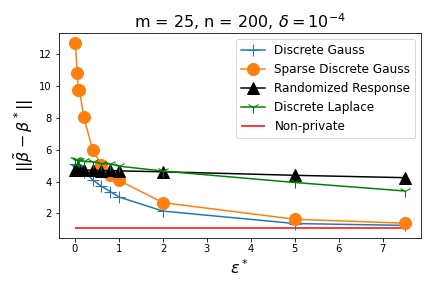
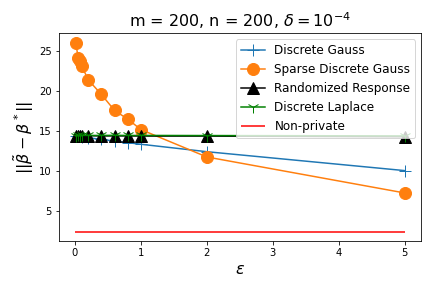
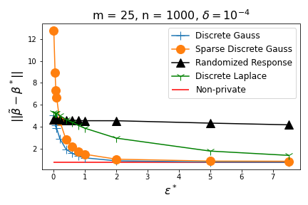
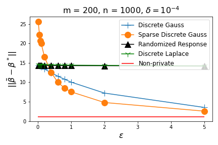
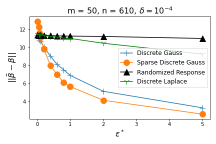
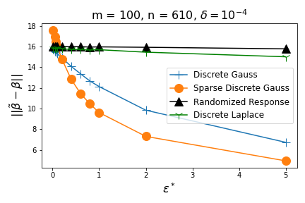
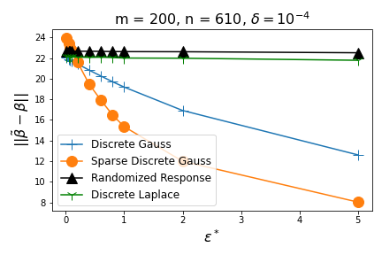
From Lemma 4.1, one can see that the variance of the additive Gaussian noise scales as the square root of the number of pairwise differential measurements. When $n\gg m$, the additive noise will be dominated by the signal from the user data and the private spectral algorithm will produce an accurate estimate (e.g., see Figure 1). On the other hand, suppose we have a large $m$ (say $m\geq 100$) but a relatively small $n$ ($n\leq 500$). Adding $\mathcal{N}_{\mathbb{Z}}\left(0,\frac{\sqrt{m(m-1)}}{\epsilon^{2}}\right)$-distributed noise to each pairwise differential measurement may introduce a lot of noise, dominating the signal and leading to a less accurate final estimate.

To overcome this limitation, we propose a heuristic modification to the private spectral algorithm. Instead of constructing a “dense” Markov chain where every pairwise transition probabilities are non-zero, we construct a sparse approximation of this Markov chain. We first generate an Erdős-Rényi graph with $m$ vertices and edge probability $p_{0}=(1+\mathchoice{\scalebox{0.9}{$\scriptstyle\mathcal{O}$}}{\scalebox{0.9}{$\scriptstyle\mathcal{O}$}}{{\scriptscriptstyle\mathcal{O}}}{\scalebox{0.7}{$\scriptscriptstyle\mathcal{O}$}}{}(1))\frac{\log m}{m}$. Note that the condition on the edge probability is to ensure that the resulting comparison graph is connected with high probability (Erdos et al.,, 1960). If we further ensure that all pairwise transition probabilities are positive, the resulting Markov chain will admit a unique stationary distribution and subsequently a unique parameter estimate. The advantage here is that we only compute $(1+\mathchoice{\scalebox{0.9}{$\scriptstyle\mathcal{O}$}}{\scalebox{0.9}{$\scriptstyle\mathcal{O}$}}{{\scriptscriptstyle\mathcal{O}}}{\scalebox{0.7}{$\scriptscriptstyle\mathcal{O}$}}{}(1))m\log m$ pairwise differential measurements. Hence for each subsampled pairwise differential measurement, we only need to add $\mathcal{N}_{\mathbb{Z}}\left(0,\frac{\sqrt{\mathcal{O}(m\log m)}}{{\epsilon^{*}}^{2}}\right)$-distributed noise and achieve the same CDP guarantee, a $\sqrt{m}$ factor reduction in variance compared to the dense Markvo chain construction.

However, sparsification might also come with its own limitation. By removing some of the pairwise transition probabilities information from the Markov chain, the final estimate obtained from the sparse Markov chain may deviate from that using full information. As our experiments will show, sparsification tradeoffs between additive noise and approximation error. It is appropriate to use sparsification to achieve a low-to-moderate privacy guarantee with good estimation accuracy when the number of items is large and the number of user is small. Finally, Algorithm 2 summarizes our private spectral algorithm.

Algorithm 2 The Private Spectral Estimator

Input: Response data $X\in\{0,1\}^{n\times m}$, $p_{0}$ (default 1) and desired privacy level $\epsilon^{*}$.
    Output: Private item estimate $\tilde{\beta}$

1:  Construct a private Markov chain $\tilde{M}$ with underlying comparison graph drawn from an Erdos-Reyni distribution with edge probability $p_{0}$ per Equation (4) and desired privacy level $\epsilon^{*}$.

2:  Follow steps 2-3 in Algorithm 1 using $\tilde{M}$.

5 EXPERIMENTS

In this section, we evaluate the privacy-accuracy tradeoff of the private spectral algorithm on synthetic and real-life datasets. We use randomized response (on the user data) and the discrete Laplace mechanism as baseline methods. Recently it has been shown that one can amplify the privacy guarantee of randomized response by shuffling the randomized user data (cf., Theorem III.1 of Feldman et al., (2022)). We compare the algorithms in terms of their approximate differential privacy guarantee . Specifically, we fix a common $\delta=10^{-4}$ and evaluate the accuracy at varying privacy levels $\epsilon^{*}$. For readers who are not familiar with privacy-preserving mechanisms, we describe these approaches in the supplementary materials and their implementation.

5.1 Synthetic Datasets.

Figure 1 shows the performance of the algorithms on synthetic datasets where we know the ground truth $\beta^{*}$. The amount of noise introduced by the discrete Gaussian mechanism gets proportionally smaller than the signal as $n$ grows. Expectedly, given a sufficiently large $n$ (relative to $m$), we see almost identical performance between the non-private estimator and the private estimator using the discrete Gaussian mechanism. At the very high privacy regime $\epsilon^{*}\approx 0.01$, all methods produce very inaccurate results. Sparsification is significantly worse than the other approaches in this regime because of the combined effect of a large amount of additive noise and the approximation error introduced by sparsification. The differences among the methods become more apparent in the low-to-moderate privacy regime. As $\epsilon^{*}$ increases, the accuracy of the discrete Gaussian mechanism improves significantly. On the other hand, randomized response and the Laplace mechanism would require either a very large $n$ or a very large privacy budget $\epsilon^{*}$ to produce a reasonably accurate estimate, neither of which is desirable.

(a) Given the same number of users, increasing $m$ expectedly leads to a worse privacy-accuracy tradeoff for all methods. The discrete Gaussian mechanism generally outperforms the baselines at the low-to-moderate privacy regime.

(b) The privacy-accuracy tradeoff for the discrete Gaussian mechanism gets better as $n$ increases (from 200 in the previous subfigure to 1000) while randomized response and the Laplace mechanism see little gain from a larger $n$.

Figure 1: Synthetic datasets. The discrete Gaussian mechanism outperforms the baselines at low-to-moderate privacy regime and enjoys substantial improvement from a larger sample size $n$.

5.2 Real-life Datasets.

For real life datasets, we do not have a ground truth $\beta^{*}$. However, previous work has shown that the spectral algorithm is competitive with the most commonly used IRT algorithms. Also considering that we focus on privacy-preservation in this work, we evaluate $\lVert\tilde{\beta}-\beta\rVert$, where $\beta$ is the output of the non-private spectral algorithm and $\tilde{\beta}$ that of the corresponding private algorithm.

Education Datasets. We include commonly used education testing datasets including LSAT (McDonald,, 2013), UCI (Hussain et al.,, 2018) and the Three Grades dataset (Cortez and Silva,, 2008). These datasets have a very small number of items. At very high privacy level $\epsilon\approx 0.01$, all methods produce very inaccurate estimate and randomized response is the most accurate method. However, at a moderate privacy level $\epsilon^{*}\approx 1$, the Laplace mechanism and the Gaussian mechanism outperform the randomized response approach. On the other hand, to produce a reasonably accurate estimate, randomized response would require a very large $\epsilon^{*}$, leading to a vacuous privacy guarantee.

(a) LSAT dataset.

(b) Three grades dataset.

(c) UCI student dataset.

Figure 2: Education datasets. The Gaussian mechanism and the Laplace mechanism outperforms randomized response at low-to-moderate privacy levels. The results here suggest that for many education testing application where the number of items is small, the spectral algorithm with the discrete Gaussian (or Laplace) mechanism should be the preferred privacy-preserving algorithm.

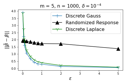
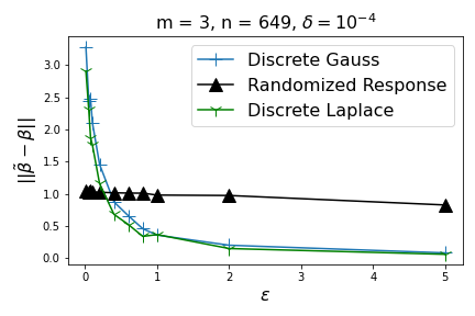
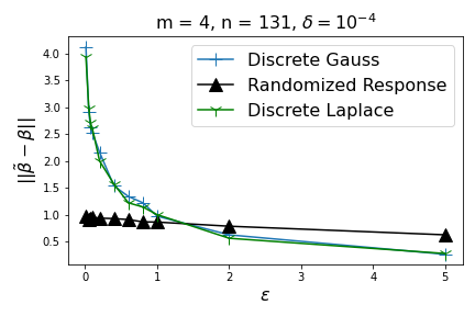
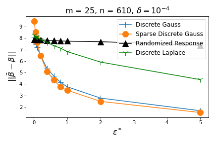
ML-100K Recommendation Systems Datasets. For experiments on recommendation systems datasets (Harper and Konstan,, 2015), we follow a similar approach to previous work to generate binary response data from ratings data (Lan et al.,, 2018; Davenport et al.,, 2014). We first perform a low rank matrix estimation of the user-item ratings matrix and use the estimation as the user-item preference scores. For each user, we convert scores that are lower than the average to 1 and scores that are higher than the average to 0. We then select a random subset of $m$ items and extract the corresponding submatrix as the response matrix. From Figure 3, one can see that the discrete Gaussian mechanism provides superi or privacy-accuracy tradeoff compared to the other approaches. Notably, sparsification provides a more accurate parameter estimation by reducing the amount of noise needed to ensure the same level of privacy and this improvement is significant when $m$ is large.

From the experiments on synthetic and real-life datasets, one can see that when we desire high accuracy and a moderate level of privacy, the discrete Gaussian mechanism should be the preferred approach. Additionally, when the number of items $m$ is large while the number of users $n$ is small, one should use the sparse Markov chain construction.

(a) When $m$ is small, sparsification doesn’t significantly improve the performance of the private spectral algorithm.

(b) With the same $n$ and a large number of items $m$, the ‘sparse Markov chain’ approach is significantly better than the ‘dense Markov chain’ approach.

Figure 3: ML-100K datasets. The discrete Gaussian mechanism generally outperforms the baselines, especially in the low-to-moderate privacy regime $\epsilon^{*}\geq 1$.

6 ETHICAL DISCUSSIONS

Our work explores privacy matters for an algorithm of which real-life applications often involve human data with sensitive information. For example, the Rasch model is often studied in the context of education testing and psychological testing where the subjects are students and patients. Therefore, deploying any algorithms in such capacity needs to be accompanied by thoughtful and thorough ethical considerations. In this work, we provide the algorithmic tool to quantify the error associated with the parameter estimates and to preserve the privacy of the human subjects.

7 CONCLUSION

In this work, we made two contributions to the understanding of the spectral algorithm for parameter estimation under the Rasch model. Firstly, we show that the spectral algorithm achieves the optimal entrywise error bound, complementing its optimal $\ell_{2}$ error guarantee obtained in the previous work. Secondly, we propose, for the first time in the item response theory literature, a differentially private algorithm. We complement our theoretical and algorithmic contributions with experimental results showing that the discrete Gaussian mechanism provides accurate parameter estimation, outperforming the baselines. A possible future extension of this work is a deeper analysis of the random subsampling of the comparison graph in the sparse discrete Gaussian mechanism. We believe that the randomized sparsification step could provide some form of privacy amplification. Furthermore, designing an accurate estimation algorithm for the high privacy regime ($\epsilon^{*}\approx 0.01$) remains an unresolved challenge.

8 ACKNOWLEDGEMENT

The authors would like to thank the anonymous reviewers for their thoughtful suggestions and comments. We thank Aaron Roth and Emily Diana of the University of Pennsylvania for fruitful discussions on the topic of differential privacy. The authors are supported by NSF Grant DMS-2112099. A.Z. acknowledges financial support from the Alfred H. Williams Faculty Scholar award. Any opinions expressed in this paper are those of the authors and do not necessarily reflect the views of the National Science Foundation.

Addressing the Reviewers’ Feedback.

In response to the anonymous reviewers’ feedback during the submission process, we have performed additional theoretical and experimental analyses and included the additional findings in the supplementary materials. Specifically, we have studied how the performance of the sparse spectral algorithm depends on the edge sampling probability $p_{0}$. We have also provided a high-level analysis of the entrywise error of the private spectral estimate, complementing Theorem 3.1.

References

- Andersen, (1973) Andersen, E. B. (1973). Conditional inference for multiple-choice questionnaires. British Journal of Mathematical and Statistical Psychology, 26(1):31–44.
- Brzezińska et al., (2016) Brzezińska, J. et al. (2016). Latent variable modelling and item response theory analyses in marketing research. Folia Oeconomica Stetinensia, 16(2):163–174.
- Bun and Steinke, (2016) Bun, M. and Steinke, T. (2016). Concentrated differential privacy: Simplifications, extensions, and lower bounds. In Theory of Cryptography Conference, pages 635–658. Springer.
- Canonne et al., (2020) Canonne, C. L., Kamath, G., and Steinke, T. (2020). The discrete gaussian for differential privacy. Advances in Neural Information Processing Systems, 33:15676–15688.
- Chen et al., (2005) Chen, C.-M., Lee, H.-M., and Chen, Y.-H. (2005). Personalized e-learning system using item response theory. Computers & Education, 44(3):237–255.
- Chen et al., (2021) Chen, Y., Li, C., and Xu, G. (2021). A note on statistical inference for noisy incomplete 1-bit matrix. arXiv preprint arXiv:2105.01769.
- Chen and Ahn, (2020) Chen, Z. and Ahn, H. (2020). Item response theory based ensemble in machine learning. International Journal of Automation and Computing, 17(5):621–636.
- Cortez and Silva, (2008) Cortez, P. and Silva, A. M. G. (2008). Using data mining to predict secondary school student performance.
- Davenport et al., (2014) Davenport, M. A., Plan, Y., Van Den Berg, E., and Wootters, M. (2014). 1-bit matrix completion. Information and Inference: A Journal of the IMA, 3(3):189–223.
- Dwork et al., (2014) Dwork, C., Roth, A., et al. (2014). The algorithmic foundations of differential privacy. Foundations and Trends® in Theoretical Computer Science, 9(3–4):211–407.
- Dwork and Rothblum, (2016) Dwork, C. and Rothblum, G. N. (2016). Concentrated differential privacy. arXiv preprint arXiv:1603.01887.
- Erdos et al., (1960) Erdos, P., Renyi, A., et al. (1960). On the evolution of random graphs. Publ. Math. Inst. Hung. Acad. Sci, 5(1):17–60.
- Feldman et al., (2022) Feldman, V., McMillan, A., and Talwar, K. (2022). Hiding among the clones: A simple and nearly optimal analysis of privacy amplification by shuffling. In 2021 IEEE 62nd Annual Symposium on Foundations of Computer Science (FOCS), pages 954–964. IEEE.
- Fischer, (1981) Fischer, G. H. (1981). On the existence and uniqueness of maximum-likelihood estimates in the rasch model. Psychometrika, 46(1):59–77.
- Ghosh et al., (2009) Ghosh, A., Roughgarden, T., and Sundararajan, M. (2009). Universally utility-maximizing privacy mechanisms. In Proceedings of the forty-first annual ACM symposium on Theory of computing, pages 351–360.
- Ghosh, (1995) Ghosh, M. (1995). Inconsistent maximum likelihood estimators for the rasch model. Statistics & Probability Letters, 23(2):165–170.
- Haberman, (1977) Haberman, S. J. (1977). Maximum likelihood estimates in exponential response models. The annals of statistics, 5(5):815–841.
- Hambleton et al., (1991) Hambleton, R. K., Swaminathan, H., and Rogers, H. J. (1991). Fundamentals of item response theory, volume 2. Sage.
- Harper and Konstan, (2015) Harper, F. M. and Konstan, J. A. (2015). The movielens datasets: History and context. Acm transactions on interactive intelligent systems (tiis), 5(4):1–19.
- Hussain et al., (2018) Hussain, S., Dahan, N. A., Ba-Alwib, F. M., and Ribata, N. (2018). Educational data mining and analysis of students’ academic performance using weka. Indonesian Journal of Electrical Engineering and Computer Science, 9(2):447–459.
- Lan et al., (2018) Lan, A., Chiang, M., and Studer, C. (2018). An estimation and analysis framework for the rasch model. In International Conference on Machine Learning, pages 2883–2891. PMLR.
- Lord, (2012) Lord, F. M. (2012). Applications of item response theory to practical testing problems. Routledge.
- Martínez-Plumed et al., (2019) Martínez-Plumed, F., Prudêncio, R. B., Martínez-Usó, A., and Hernández-Orallo, J. (2019). Item response theory in ai: Analysing machine learning classifiers at the instance level. Artificial intelligence, 271:18–42.
- McDonald, (2013) McDonald, R. P. (2013). Test theory: A unified treatment. psychology press.
- Mironov, (2012) Mironov, I. (2012). On significance of the least significant bits for differential privacy. In Proceedings of the 2012 ACM conference on Computer and communications security, pages 650–661.
- Moraes et al., (2020) Moraes, J. V., Reinaldo, J. T., Prudencio, R. B., and Silva Filho, T. M. (2020). Item response theory for evaluating regression algorithms. In 2020 International Joint Conference on Neural Networks (IJCNN), pages 1–8. IEEE.
- Nguyen and Zhang, (2022) Nguyen, D. and Zhang, A. (2022). A spectral approach to item response theory. Advances in neural information processing systems, 35.
- Rasch, (1960) Rasch, G. (1960). Studies in mathematical psychology: I. probabilistic models for some intelligence and attainment tests.
- Schellhorn and Sharma, (2013) Schellhorn, C. and Sharma, R. (2013). Using the rasch model to rank firms by managerial ability. Managerial Finance.
- Van der Linden and Hambleton, (1997) Van der Linden, W. J. and Hambleton, R. (1997). Handbook of item response theory. Taylor & Francis Group. Citado na pág, 1(7):8.
- Warner, (1965) Warner, S. L. (1965). Randomized response: A survey technique for eliminating evasive answer bias. Journal of the American Statistical Association, 60(309):63–69.
- Whitehill et al., (2009) Whitehill, J., Wu, T.-f., Bergsma, J., Movellan, J., and Ruvolo, P. (2009). Whose vote should count more: Optimal integration of labels from labelers of unknown expertise. Advances in neural information processing systems, 22.