CHGNN: A Semi-Supervised Contrastive Hypergraph Learning Network

Abstract

Hypergraphs can model higher-order relationships among data objects that are found in applications such as social networks and bioinformatics. However, recent studies on hypergraph learning that extend graph convolutional networks to hypergraphs cannot learn effectively from features of unlabeled data. To such learning, we propose a contrastive hypergraph neural network, CHGNN, that exploits self-supervised contrastive learning techniques to learn from labeled and unlabeled data. First, CHGNN includes an adaptive hypergraph view generator that adopts an auto-augmentation strategy and learns a perturbed probability distribution of minimal sufficient views. Second, CHGNN encompasses an improved hypergraph encoder that considers hyperedge homogeneity to fuse information effectively. Third, CHGNN is equipped with a joint loss function that combines a similarity loss for the view generator, a node classification loss, and a hyperedge homogeneity loss to inject supervision signals. It also includes basic and cross-validation contrastive losses, associated with an enhanced contrastive loss training process. Experimental results on nine real datasets offer insight into the effectiveness of CHGNN, showing that it outperforms 13 competitors in terms of classification accuracy consistently.

1 Introduction

Hypergraphs generalize graphs by introducing hyperedges to represent higher-order relationships among groups of nodes. This representation is highly relevant in many real-world applications, e.g., ones that capture research collaborations. By modeling higher-order relationships, hypergraphs can provide better performance than graph-based models in many data mining tasks [1, 2]. Recently, hypergraphs have been applied in diverse domains, including social networks [3], knowledge graphs [4], e-commerce [5], and computer vision [6]. These applications illustrate the versatility and potential of hypergraphs as a tool for capturing complex relationships among objects.

Like graph problems (e.g., node classification and link prediction), where machine learning, especially deep learning, has yielded state-of-the-art solutions, many hypergraph problems [6, 7] are being solved by neural network-based models. In this paper, we study a fundamental problem in using neural networks for hypergraphs, which is to learn node representations for downstream tasks. The goal is to preserve the structure and attribute features of nodes in their learned embeddings so that prediction tasks based on these embeddings can be solved with higher accuracy.

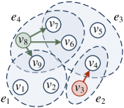
(a) HyperGNNs

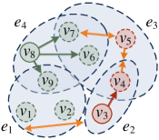
(b) CHGNN

Figure 1: Comparison of HyperGNN and CHGNN learning, where (i) colored, solid circles denote nodes with class labels; (ii) colored, dashed circles denote nodes with model-inferred classes; (iii) uncolored circles denote nodes with model-inferred classes but that are not involved in the loss calculation; (iv) dashed regions denote hyperedges; (v) red and green arrows denote class label information propagation; and (vi) orange arrows denote contrastive information propagation.

Since hypergraphs generalize graphs and graph learning studies [8, 9, 10] have shown strong results, a natural approach is to convert a hypergraph into a standard graph and apply graph neural networks (GNNs) to learn node representations. However, this approach leads to poor outcomes, to be shown in the experiments (see Section 5). This is because converting a hypergraph into a standard graph requires decomposing higher-order relations into pairwise relations, which causes a substantial information loss. To avoid this issue, recent studies instead extend GNNs to hypergraphs, obtaining so-called hypergraph neural networks (HyperGNNs). Such models first aggregate node features and then generate node representations with those of their incident hyperedges [11, 1, 2]. The aggregation process relies on hypergraph convolution, which propagates training signals obtained from node labels.

Example 1.

Fig. 1 (a) shows an example of HyperGNN learning involving nine nodes $v_{i}\,(1\leq i\leq 9)$. In a semi-supervised setting, where all nodes are only partially labeled, nodes without labels, i.e., $v_{1}$, $v_{2}$, $v_{4}$, $v_{5}$, $v_{6}$, $v_{7}$, and $v_{9}$, do not participate in the loss calculation and contribute very little to the learning process. The training loss is calculated based only on the labeled nodes, i.e., $v_{3}$ and $v_{8}$. Consequently, the representation learning outcome is sub-optimal, to be studied experimentally (see Section 5).

Motivated by the recent success of contrastive learning (CL) [12], a self-learning technique, we propose to combine contrastive and supervised learning, in order to exploit both labeled and unlabeled data better. However, this task is non-trivial and presents two main challenges.

Challenge I: How to generate a good set of hypergraph views for CL? In CL, two views are typically created by augmenting the original input data and the model learns from both views. However, since the views are derived from the same input, there is a risk that they are very similar, which will reduce performance. Thus, it is crucial to design the view generation so that the views offer diverse and informative perspectives on the input data. Existing graph and hypergraph CL data augmentation strategies [13, 14, 15] that drop edges randomly to form views suffer from information loss when being applied to hypergraphs. This is because a hyperedge often represents a complex relationship among multiple nodes, meaning that randomly dropping a hyperedge makes it difficult for affected nodes to retain their full relationship features. In addition, these views usually contain classification-independent information to varying degrees, which distracts from the key information during embedding learning.

Challenge II: How to retain the homogeneity of hyperedges when encoding hypergraph views for CL? The homogeneity of a hyperedge captures the relatedness of the nodes that form the hyperedge. Retaining the homogeneity of hyperedges in encodings is crucial to maintain the dependencies among the nodes, which can benefit downstream tasks such as node classification. Thus, the distances between the embeddings of nodes in a hyperedge with high homogeneity should be small due to the high structural similarity. However, existing hypergraph CL models [16, 17] disregard this property, negatively impacting the quality of their learned embeddings.

To tackle the above challenges, we propose a constrastive hypergraph neural network (CHGNN). First, we propose an adaptive hypergraph view generator that utilizes the InfoMin principle [18] to generate a good set of views. These views share minimal information necessary for downstream tasks. Second, we introduce a method to encode nodes and hyperedges based on the homogeneity of hyperedges. Hyperedges with strong homogeneity are given higher weights during the aggregation step of nodes. Third, we design joint contrastive losses that include basic and cross-validation contrastive losses to (i) reduce the embedding distance between nodes in the same hyperedge and nodes of the same class, and (ii) verify the distribution embeddings using correlations between nodes and hyperedges, nodes and clusters, and hyperedges and clusters. Finally, to obtain more class-tailored representations, we adaptively adjust the contrastive repulsion on negative samples during training.

Example 2.

Fig. 1 (b) provides an example of the CHGNN learning process, where we introduce more supervision signals by inferring the classes of unlabeled nodes. For example, we encourage (i) two nodes of the same class, e.g., $v_{4}$ and $v_{5}$, to learn embeddings with small distances in the embedding space; (ii) nodes of different classes, e.g., $v_{5}$ and $v_{7}$, to learn embeddings with large distances; and (iii) different hyperedges $e_{i}\,(1\leq i\leq 4)$ to learn embeddings with large distances.

Example 2 suggests the advantages of CHGNNs over HyperGNNs. We summarize the contributions as follows.

• We propose CHGNN, a novel model for hyperedge representation learning that is based on contrastive and semi-supervised learning. The unique combination of these two strategies enables CHGNNs to exploit both labeled and unlabeled data during learning, enabling better accuracy in prediction tasks.

• To enable contrastive hypergraph learning, we propose an adaptive hypergraph view generator that learns hyperedge-level augmentation policies in a data-driven manner, which provides sufficient variances for contrastive learning. Moreover, we present a hyperedge homogeneity-aware HyperGNN (H-HyperGNN) that takes into account the homogeneity of hyperedges when performing encoding.

• We propose a joint loss function that combines a similarity loss for view generators and supervision losses with two contrastive loss terms: basic and cross-validation contrastive losses for H-HyperGNN. They enable CHGNN to learn from both labeled and unlabeled data.

• We design an enhanced contrastive loss training strategy that enables the adaptive adjustment of the temperature parameter of negative samples in the loss function. The strategy gradually decreases the similarity between instances of different classes during training.

• We evaluate CHGNN on nine real datasets, finding that CHGNN consistently outperforms thirteen state-of-the-art proposals, including semi-supervised learning and contrastive learning methods, in terms of classification accuracy. The superior performance across all datasets demonstrates the robustness of CHGNN.

We proceed to review related work in Section 2 and to introduce preliminaries in Section 3. Section 4 presents CHGNN, and Section 5 covers the experimental study. Section 6 concludes and offers research directions.

2 Related Work

2.1 Hypergraph Neural Networks

Hypergraph neural networks represent a promising approach to analyzing hypergraph-structured data. The basic idea of hypergraph neural networks is that nodes in the same hyperedge are often similar and hence are likely to share the same label [19].

HGNN [1], the first proposal of a HyperGNN method, performs convolution with a hypergraph Laplacian that is further approximated by truncated Chebyshev polynomials. HyperConv [20] proposes propagation between nodes that exploits higher-order relationships and local clustering structures in these. HyperGCN [2] further uses a generalized hypergraph Laplacian with mediators to approximate the input hypergraph. MPNN-R [21] treats hyperedges as a new node type and connects a “hyperedge node” with all nodes that form the hyperedge. This converts a hypergraph into a graph, to which GNNs apply directly. AllSet [22] integrates Deep Set and Set Transformer with HyperGNNs for learning two multiset functions that compose the hypergraph neural network layers. HyperSAGE [23] exploits the structure of hypergraphs by aggregating messages in a two-stage process, which avoids the conversion of hypergraphs into graphs and the resulting information loss. HNHN [24] extends a hypergraph to a star expansion by using two different weight matrices for node- and hyperedge-side message aggregation. UniGNN [11] provides a unified framework that generalizes the message-passing processes for both GNNs and HyperGNNs. Studies of HyperGNNs also exist that target tasks other than classification, e.g., hyperedge prediction [25], and that target other types of hypergraphs, e.g., recursive hypergraphs [21, 26], which are not comparable to CHGNN.

Despite the promising results obtained by the existing methods, their message-passing is limited to nodes within only a few hops. This becomes a challenge when the input graph is sparsely labeled, as the methods may fail to obtain sufficient supervision signals for many unlabeled nodes, making them unable to learn meaningful representations for such nodes. Although heterogeneous GNNs [27, 28] may appear to be applicable to hypergraph tasks, by converting hypergraphs into bipartite graphs, they are not suited for such tasks. They focus primarily on extracting semantic information from different meta-paths, which is not relevant for hypergraphs that have only one meta-path. Furthermore, experiments [22] show that (i) heterogeneous GNNs perform significantly worse than HyperGNNs; and (ii) heterogeneous GNNs do not scale well even to moderately sized hypergraphs.

2.2 Contrastive Graph Neural Networks

Contrastive learning (CL) is a self-supervised technique that learns representations by minimizing the distances between embeddings of similar samples and by maximizing the distances between those of dissimilar samples. Graph contrastive learning (GCL) applies the idea of CL to GNNs. Some GCL models calculate a node-level contrastive loss function between nodes and the entire graph [13], high-level hidden representations [29] or subgraphs [30] without an augmentation. Alternatively, some GCL models generate contrastive samples, known as graph views, through data augmentation techniques, e.g., edge perturbation [14, 31, 32], subgraph sampling [14, 33], feature masking [14, 31, 32], learnable view generators [34], and model parameter perturbation [35]. As SimGRACE [35] and DGI [13] have achieved state-of-the-art results with and without augmentation in graph representation learning, we include them in Section 5.

GCL models, despite their effectiveness in processing graphs, are not suitable for hypergraphs for two main reasons. First, applying GCL models to hypergraphs necessities the conversion from hypergraphs to general graphs, resulting in significant information loss, to be demonstrated in Section 5. Second, their data augmentation strategies do not take into account hypergraphs and are thus unable to capture higher-order information by general edges. CHGNN, on the other hand, possesses an adaptive hypergraph view generator. It assigns unique augmentation operations to each hyperedge and utilizes the overlap between hyperedges to mask nodes in a node-specific manner.

The application of contrastive learning to hypergraphs is still evolving, with TriCL [15] being the state-of-the-art and representative model. TriCL introduces a tri-directional contrast mechanism that combines contrasting node, group, and membership labels to learn node embeddings. TriCL outperforms not only unsupervised baselines but also models trained with labeled supervision. Xia et al. [16] improve session-based recommendations by maximizing mutual information between representations learned. Zhang et al. [17] address data sparsity in group recommendations by using the contrast between coarse-grained and fine-grained hypergraphs. HCCF [4] learns user representations by aligning explicit user-item interactions with implicit hypergraph-based dependencies for collaborative filtering. These models [16, 17, 4] (i) only learn embeddings on heterogeneous social hypergraphs for non-classification tasks; and (ii) they capture differences between individual nodes rather than between nodes of different classes as a whole, as they target recommendation. As a result, they are fundamentally different from and incomparable to CHGNNs.

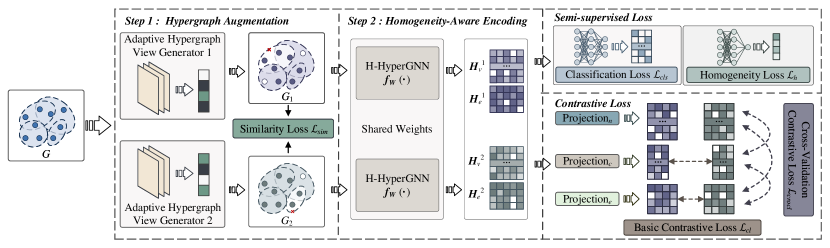
Figure 2: CHGNN model overview.

3 Preliminaries

Definition 1.

A hypergraph is denoted as $G=(V,E)$, where $V=\{v_{1},v_{2},\ldots,v_{n}\}$ is a node set and $E\subseteq 2^{V}$ is a hyperedge set. Each hyperedge $e\in E$ is a non-empty subset of $V$.

Definition 2.

Given a hypergraph $G=(V,E)$, the egonet $E_{\{v_{i}\}}$ of a node $v_{i}\in V$ is the set of hyperedges that contain $v_{i}$.

Clearly, the higher $E_{\{v_{i}\}}$, the higher the connectivity of $v_{i}$ in the hypergraph. Fig. 1 (a) shows a hypergraph $G=(V,E)$, where $V=\{v_{1},v_{2},v_{3},v_{4},v_{5},v_{6},v_{7},v_{8},v_{9}\}$, $E=\{e_{1},e_{2},e_{3},e_{4}\}$. $e_{1}=\{v_{1},v_{2},v_{9}\}$, $e_{2}=\{v_{3},v_{4}\}$, $e_{3}=\{v_{4},v_{5},v_{6},v_{7}\}$, and $e_{4}=\{v_{6},v_{7},v_{8},v_{9}\}$. Further, $E_{\{v_{9}\}}=\{e_{1},e_{4}\}$ due to $v_{9}\in e_{1}\cap e_{4}$.

Definition 3.

The feature matrix of a hypergraph $G=(V,E)$ is denoted as $\bm{X}\in\mathbb{R}^{|V|\times F}$, where each row $\bm{x}_{i}$ of $\bm{X}$ is an $F$-dimensional feature vector of a node $v_{i}$.

Definition 4.

The class label vector of a hypergraph $G=(V,E)$ is denoted as $\bm{y}\in\mathbb{N}^{|V|}$, where each element $y_{i}$ of $\bm{y}$ represents the class label of $v_{i}$ and $\mathbb{N}$ is a set of natural numbers.

Definition 5.

The homogeneity [36] of a hyperedge $e\in E$, denoted $homo(e)$ is given by:

$$homo(e):=\begin{cases}\sigma(\frac{\sum_{\{v_{i},v_{j}\}\in\binom{e}{2}}|E_{\{v_{i}\}}\cap E_{\{v_{j}\}}|}{|\binom{e}{2}|})&\text{if }|e|>1\\ 1&\text{otherwise},\end{cases}\vspace{-1mm}$$ (1)

where $\binom{e}{2}$ is the set of node pairs in $e$, $|\binom{e}{2}|$ is the cardinality of $\binom{e}{2}$, $|E_{\{v_{i}\}}\cap E_{\{v_{j}\}}|$ is the degree of pair $\{v_{i},v_{j}\}$, and $\sigma(\cdot)$ is the sigmoid function.

Homogeneity measures the strength of the dependencies between the nodes in a hyperedge. A high homogeneity of a hyperedge $e$ means that pairs of nodes in $e$ appear frequently in the edge set $E$. This indicates a strong dependency and a high likelihood of similar attributes (e.g., labels) among all node pairs.

Definition 6.

Give a hypergraph $G=(V,E)$, the feature matrix $\bm{X}$ of $G$ and the labeled set $V_{L}$ ($|V_{L}|\ll|V|$) with the label set $Y_{L}=\{y_{i}|v_{i}\in V_{L}\}$, contrastive hypergraph neural network (CHGNN) performs transductive graph-based semi-supervised learning for semi-supervised node classifiction, where the labeled set $Y_{un}=\{y_{j}|v_{j}\in V-V_{L}\}$ is identified.

4 CHGNN

4.1 Model Overview

CHGNN follows the common two-branch framework of GCL models [14] and encompasses two steps: hypergraph augmentation and homogeneity-aware encoding, as shown in Fig. 2.

Hypergraph augemtation. The input hypergraph $G=(V,E)$ is augmented to obtain $G_{1}=(V_{1},E_{1})$ and $G_{2}=(V_{2},E_{2})$ (cf. Fig. 2) using two adaptive hypergraph view generators. We detail the hypergraph augmentation in Section 4.2.

Homogeneity-aware encoding. The two augmented hypergraph views, $G_{1}$ and $G_{2}$, are fed separately into two hyperedge homogeneity-aware HyperGNNs (H-HyperGNNs) to encode the nodes and hyperedges into latent spaces, described in Section 4.3.

Loss function. We propose a loss function that encompasses two semi-supervised and two contrastive loss terms. The semi-supervised loss utilizes label and hyperedge homogeneity information to generate supervision signals that propagate to unlabeled nodes during training. The basic contrastive loss terms force embeddings of the same cluster (and hyperedge) computed from $G_{1}$ and $G_{2}$ to be similar, while embeddings of different clusters (and hyperedges) are expected to be dissimilar. The cross-validation contrastive loss maximizes the embedding agreement between the nodes, the clusters, and the hyperedges. We detail the loss function in Section 4.4.

Enhance training. We apply increased repulsion to the negative samples that are difficult to distinguish by adjusting the temperature parameters so that nodes can obtain more class-tailored representations with limited negative samples. The enhanced training process is covered in Section 4.5.

4.2 Hypergraph Augmentation

Hypergraph augmentation is essential for creating hypergraph views that preserve the topological structure of the hypergraph and maintain the node labels. We propose augmentation schemes that maintain significant topological and semantic information of hypergraphs for classification, thereby improving CL performance.

4.2.1 Adaptive Hypergraph View Generator

Fig. 3 depicts the framework of the adaptive hypergraph view generator. Given a hypergraph $G$, we generate two hypergraph views $G_{1}$ and $G_{2}$ by perturbing $G$ with three operations: preserve hyperedges (P), remove hyperedges (R), and mask some nodes in the hyperedges (M). Note that graph augmentation typically includes removing nodes and masking node features in addition to the above operations. However, perturbation of nodes does not apply to hypergraphs due to their hyperedges that represent higher-order relationships rather than the pairwise relationships. Directly perturbing a node interferes with the aggregation of $d_{v}~{}\times~{}d_{e}$ neighbor nodes, while perturbing a hyperedge only affects $d_{e}$, where $d_{v}$ and $d_{e}$ is the average node and hyperedge degree in a hypergraph, respectively. To preserve the original topological and semantic information and retain greater variance, we employ finer-grained hyperedge perturbation instead of node perturbation.

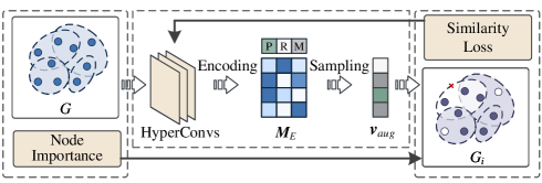
Figure 3: Adaptive hypergraph view generator framework.

We use the HyperConv layers [20] to obtain the hyperedge embedding matrix $\bm{M}_{E}$ by iteratively aggregating nodes and hyperedges. Each hyperedge embedding represents the probabilities of preserving, removing, and masking operations. We employ the Gumbel-softmax [37] to sample from these probabilities, and then the output $\bm{v}_{aug}$ assigns an augmentation operation to each hyperedge. We mask a node $v_{i}$ based on its importance during the masking operation.

4.2.2 Overlappness-based Masking

To maintain the semantics (i.e., class) of node labels during hypergraph augmentation, two masking principles should be followed. First, a node is considered more important if its egonet contains more distinct nodes. Second, if the hyperedges contained in the egonet of a node overlap less with the hyperedges contained in the egonets of other nodes, the node is considered more important. We provide an example to illustrate the two principles.

Example 3.

In Fig. 1 (a), $E_{\{v_{9}\}}=\{e_{1},e_{4}\}$ contains 6 nodes: $v_{1}$, $v_{2}$, $v_{6}$, $v_{7}$, $v_{8}$, $v_{9}$, while $E_{\{v_{4}\}}=\{e_{2},e_{3}\}$ contains 5 nodes: $v_{j}$ ($3\leq j\leq 7$). In this case, masking node $v_{9}$ results in higher information loss than masking node $v_{4}$. Second, the number of nodes contained in $E_{\{v_{6}\}}=\{e_{3},e_{4}\}$ is 6, which is the same as for $E_{\{v_{9}\}}$. However, $v_{6}$ is less important than $v_{9}$ because (i) $E_{\{v_{6}\}}=E_{\{v_{7}\}}$, meaning that $e_{3}$ and $e_{4}$ can still be connected via $v_{7}$ even if $v_{6}$ is masked; and (ii) $E_{\{v_{9}\}}\cap E_{\{v_{1}\}}=\{e_{1}\}\neq E_{\{v_{9}\}}$, and $E_{\{v_{9}\}}\cap E_{\{v_{8}\}}=\{e_{4}\}\neq E_{\{v_{9}\}}$, meaning that $e_{1}$ and $e_{4}$ cannot be connected if $v_{9}$ is masked.

We introduce the overlappness [36] of an egonet to evaluate the significance of a node $v_{i}$ in line with the above two principles.

Definition 7.

The overlappness of the egonet of $v_{i}$, denoted by $o(v_{i})$, is defined as:

$$o(v_{i}):=\frac{\sum_{e\in E_{\{v_{i}\}}}|e|}{|\bigcup_{e\in E_{\{v_{i}\}}}e|}$$ (2)

When the number of distinct nodes in the egonet of $v_{i}$ is large, or the hyperedges in the egonet of $v_{i}$ overlap less, the value of $o(v_{i})$ is small, i.e., the node is more important (cf. Formula 2). To normalize overlapness values, which may vary considerably, we use $w_{v_{i}}=\log o(v_{i})$. Next, we apply it to compute the probability of masking $v_{i}$.

$$p_{v_{i}}=\min\{\frac{w_{nmax}-w_{v_{i}}}{w_{nmax}-w_{navg}}\cdot p_{node},p_{\tau}\},\vspace{-2mm}$$ (3)

where $p_{node}$ is a hyperparameter that determines the overall probability of masking any node (i.e., the sparsity of the resulting views), $w_{nmax}$ and $w_{navg}$ are the maximum and average of the normalized overlappness in $G$, and $p_{\tau}$ is a cut-off probability.

4.2.3 View Generator Training

A good set of views should share only the minimal information needed for high performance on a classification task. In line with this, we train a view generator in an end-to-end manner to generate task-dependent views, allowing the classification loss to guide the generator to retain classification information. A similarity loss is used to minimize the mutual information between the views generated by following [18]. The similarity between the views is measured by comparing the outputs of the view generators:

$$\mathcal{L}_{sim}=sim(\bm{v}_{aug}^{1},\bm{v}_{aug}^{2}),\vspace{-1mm}$$ (4)

where $\bm{v}_{aug}^{1}$ and $\bm{v}_{aug}^{2}$ are the augmentation vectors for generators $G_{1}$ and $G_{2}$ in Fig. 2, respectively, and $sim(\cdot)$ is the similarity loss. In this paper, we adopt the mean squared error loss.

4.3 Hyperedge Homogeneity-aware HyperGNN

The aggregation process above treats all hyperedges containing a node $v_{i}$ equally and ignores their semantic differences.

Example 4.

Consider a publication domain classification problem as shown in Fig. 4, where nodes represent papers and colors represent different domains (e.g., artificial intelligence), and where papers in the same hyperedge have the same author. Nodes $v_{i}$, $v_{1}$, and $v_{2}$ represent papers with the same author because they belong to the same hyperedge ($e_{1}$). When updating the embedding of $v_{i}$ for subsequent classification, existing HyperGNNs treat $e_{1}$, $e_{2}$, and $e_{3}$ equally (see Fig. 4 (a)). However, $e_{2}$ should be given lower weight, as it contains nodes from distinct domains and has more diverse semantics (see Fig. 4 (b)). Specifically, when an author publishes in diverse domains, there is a higher uncertainty regarding which domain a paper by the author belongs to.

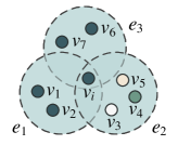
(a) Equal aggregation

(b) Ideal aggregation

Figure 4: Aggregation based on homogeneity.

The above example suggests that it is crucial to take into account the semantic information of hyperedges. Motivated by this, we propose an H-HyperGNN that weighs the hyperedges by their homogeneity of semantic information. We propagate the features as follows:

$$\begin{split}\bm{h}_{e,e_{i}}^{(l)}&=\frac{1}{|e_{i}|}\sum_{v_{j}\in e_{i}}\bm{h}_{v,v_{j}}^{(l-1)}\\ \bm{h}_{v,v_{i}}^{(l)}&=\bm{W}(\bm{h}^{(l-1)}_{v,v_{i}}+\sum_{e_{j}\in E_{\{v_{i}\}}}homo(e_{j})\cdot\bm{h}_{e,e_{j}}^{(l)}),\end{split}$$ (5)

where $\bm{W}$ is a learnable parameter matrix and $homo(e)$ denotes the homogeneity of a hyperedge $e\in E$, which is calculated following Formula 1. Next, $\bm{h}_{e,e_{i}}^{(l)}$ and $\bm{h}_{v,v_{i}}^{(l)}$ denote the embeddings of $e_{i}$ and $v_{i}$ at the $l$-th iteration, where $\bm{h}_{v,v_{i}}^{(0)}=\bm{x}_{i}$ and $\bm{x}_{i}$ is the input feature vector of $v_{i}$. We use a two-layer H-HyperGNN in our experiments (see Section 5). The final layer output of the H-HyperGNN forms the learned embeddings of the nodes and hyperedges, which are used for loss computation in the next stage.

4.4 Model Training

4.4.1 Semi-Supervised Training Loss

Classification loss. The final embedding of each labeled node $v_{i}$ is computed by taking the average of its two embedding vectors $\bm{h}_{v,v_{i}}^{1}$ and $\bm{h}_{v,v_{i}}^{2}$ obtained from $\bm{H}_{v}^{1}$ and $\bm{H}_{v}^{2}$ generated from $G_{1}$ and $G_{2}$ (see Fig. 2). The final embedding is then input into a classifier network (we use a two-layer MLP for simplicity) $\mathcal{C}(\cdot)$, where the cross-entropy loss is used as the classification loss.

$$\mathcal{L}_{cls}=-\sum_{v_{i}\in V_{L}}y_{i}\ln\mathcal{C}(\frac{\bm{h}_{v,v_{i}}^{1}+\bm{h}_{v,v_{i}}^{2}}{2}),$$ (6)

where $V_{L}$ is the set of labeled nodes and $y_{i}$ is the label of node $v_{i}$.

Hyperedge homogeneity loss. We denote the hyperedge embedding of view $G_{i}$ by $\bm{H}^{i}_{e}$, $i\in\{1,2\}$. We feed $\bm{H}_{e}^{i}$ into a regressor $\mathcal{R}(\cdot)$ to predict the homogeneity of all hyperedges based on their embeddings and then compute the homogeneity loss. Since hyperedge embeddings are generated by node aggregation, homogeneity can be viewed as a measure of node similarity within a hyperedge. The homogeneity loss aims to decrease the similarity between node embeddings in heterogeneous hyperedges and increase the similarity in homogeneous hyperedges. To achieve this, we compute the mean squared error between the true and predicted homogeneity values as the hyperedge homogeneity loss.

$$\mathcal{L}_{h}=\lambda_{h}\cdot(\frac{1}{2}\sum_{i\in\{1,2\}}\mathit{MSE}(\mathcal{R}(\bm{H}_{e}^{i}),\bm{v}_{homo})),\vspace{-2mm}$$ (7)

where $\lambda_{h}>0$ is a hyperparameter that weighs the importance of hyperedge homogeneity loss, $\bm{H}_{e}^{i}$ is the hyperedge embedding matrix generated from view $G_{i}$, and $\bm{v}_{homo}$ is the homogeneity vector of $E$. The $j$-th element of $\bm{v}_{homo}$ is denoted as $homo(e_{j})$.

4.4.2 Contrastive Loss

We define the output matrix in CL.

Definition 8.

$\bm{Z}_{b}^{a}$ is an output matrix of a projection head, where $a\,(\in\{1,2\})$ denotes views and $b\,(\in\{e,c,n\})$ denotes the type of projection. Further $c$ represents cluster projection, $e$ represents hyperedge projection, and $n$ represents node projection. $\bm{Z}_{b:i}^{a}$ denotes the $i$-th column of $\bm{Z}_{b}^{a}$, and $\bm{z}_{b,w}^{a}$ denotes the vector of $w$ in $\bm{Z}_{b}^{a}$.

For example in Fig. 5, $\bm{Z}^{1}_{c}$ denotes the cluster projection matrix of view $G_{1}$, and $\bm{Z}^{2}_{e}$ denotes the hyperedge projection matrix of view $G_{2}$. Next, $\bm{z}_{e,e_{1}}^{1}$ denotes the vector of $e_{1}$ in $\bm{Z}^{1}_{c}$ (i.e., the row in the brown square of Fig. 5 (b)), and $\bm{Z}_{c:1}^{1}$ denotes the first column of $\bm{Z}^{1}_{c}$ (i.e., the column in the brown square of Fig. 5 (a)).

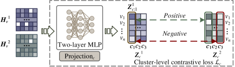
(a) Cluster-level contrastive loss

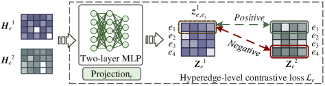
(b) Hyperedge-level contrastive loss

Figure 5: An example of basic contrastive loss.

Basic contrastive loss. Basic contrastive loss is similar to GCL [14, 33, 31, 38, 34] that contrasts the same data from different views. Two used contrastive loss notions are used commonly: node-level contrastive loss [14, 31, 33] and cluster-level contrastive loss [39]. The former aims to distribute nodes uniformly in the hyperplane, while the latter focuses on clustering nodes with similar categories and separating nodes with different categories. Clearly, the latter aligns with the objective of classification, while the former does not. Thus, we include cluster-level contrastive loss in the basic contrastive loss but exclude node-level contrastive loss. Inspired by InfoNCE loss [40], we propose a hyperedge-level contrastive loss to enhance the hyperedge embeddings. We thus incorporate also hyperedge-level contrastive loss in the basic contrastive loss.

(i) Cluster-level contrastive loss. This loss compares the cluster membership probability distributions learned from different views for each node. To get cluster membership probability distributions, $\bm{H}_{v}^{1}$ and $\bm{H}_{v}^{1}$ are loaded into a cluster projection to obtain cluster matrices $\bm{Z}_{c}^{1}$ and $\bm{Z}_{c}^{2}$. We treat the distributions of the same cluster as positive samples (e.g., cluster $c_{1}$ in $\bm{Z}_{c}^{1}$ vs. cluster $c_{1}$ in $\bm{Z}_{c}^{2}$ in Fig. 5 (a)). Conversely, the cluster membership probability distributions of different nodes learned from different views are treated as negative samples (e.g., cluster $c_{1}$ in $\bm{Z}_{c}^{1}$ vs. cluster $c_{3}$ in $\bm{Z}_{c}^{2}$ in Fig. 5 (a)), to differentiate between node clusters rather than nodes. Ideally, each node cluster should correspond to nodes of the same class. To achieve this, we project node embeddings into a space with dimensionality equal to the number of data classes (i.e., the target number of clusters). In particular, the projection is carried out using a two-layer MLP, i.e., the projection head in Fig. 5 (a). The $i$-th dimension value represents the probability of a node belonging to the $i$-th class.

Let $\bm{Z}_{c}^{1}$ and $\bm{Z}_{c}^{2}$ be the output matrix of the projection head $\mathcal{P}(\cdot)$ for the node embeddings, i.e., $\bm{Z}_{c}^{i}=\mathcal{P}(\bm{H}_{v}^{i}),i=\{1,2\}$. The cluster-level contrastive loss [39] is:

$$\mathcal{L}_{c}=\frac{1}{2C}\sum_{i=1}^{C}(\ell_{c}^{1}(\bm{Z}^{1}_{c:i})+\ell_{c}^{2}(\bm{Z}^{2}_{c:i})),\vspace{-1mm}$$ (8)

where $C$ is the number of clusters. Formula 8 aims to achieve two goals. First, for any $i\in[1,C]$, $\bm{Z}_{c:i}^{1}$ is very similar to $\bm{Z}_{c:i}^{2}$, i.e., a node $v_{j}$ from the input hypergraph has a similar probability of falling into the $i$-th class, regardless of whether its embedding is learned from $G_{1}$ or $G_{2}$. Second, $\bm{Z}_{c:i}^{1}$ and $\bm{Z}_{c:j}^{2}$ should be dissimilar when $i\neq j$ because a node should have dissimilar probabilities of falling into different classes. Formula 8 is an average of the cluster contrastive losses $\ell_{c}^{1}$ and $\ell_{c}^{2}$ computed from the two views. Since the two loss terms are symmetric, we only show $\ell_{c}^{1}(\bm{Z}^{1}_{c:i})$:

$$\ell_{c}^{1}(\bm{Z}^{1}_{c:i})=-\log\frac{\exp(s(\bm{Z}^{1}_{c:i},\bm{Z}^{2}_{c:i})/\tau_{c})}{\sum_{j=1}^{C}\exp(s(\bm{Z}^{1}_{c:i},\bm{Z}^{2}_{c:j})/\tau_{c})}$$ (9)

Here, $\tau_{c}$ is a temperature parameter corresponding to $\ell_{c}^{1}$ that controls the softness of the contrasts among positive and negative sample pairs, and $s(\cdot)$ is a vector similarity function — we use inner product.

(ii) Hyperedge-level contrastive loss. This loss aims to maximize the mutual information of hyperedge representations between different views. We project hyperedge embeddings $\bm{H}_{e}^{1}$ and $\bm{H}_{e}^{2}$ with the projection head (the two-layer MLP in Fig. 5 (b)) and output $\bm{Z}_{e}^{1}$ and $\bm{Z}_{e}^{2}$. For a hyperedge $e_{i}$, $\bm{z}^{1}_{e,{e_{i}}}$ and $\bm{z}^{2}_{e,e_{i}}$ form a positive sample pair (e.g., edge $e_{1}$ in $\bm{Z}_{e}^{1}$ vs. edge $e_{1}$ in $\bm{Z}_{e}^{2}$), while the projected embeddings of different hyperedges from different views form the negative sample pairs (e.g., edge $e_{1}$ in $\bm{Z}_{e}^{1}$ vs. edge $e_{3}$ in $\bm{Z}_{e}^{2}$). We thus define the hyperedge-level contrastive loss as:

$$\mathcal{L}_{e}=\frac{1}{2|E|}\sum_{e_{i}\in E}(\ell_{e}^{1}(\bm{z}^{1}_{e,e_{i}})+\ell_{e}^{2}(\bm{z}^{2}_{e,e_{i}}))\vspace{-1mm}$$ (10)

Similar to the cluster-level loss, $\ell_{e}^{1}$ and $\ell_{e}^{2}$ in Formula 10 denote the hyperedge contrastive losses of the two views. We thus only show $\ell_{e}^{1}(\bm{z}^{1}_{e,e_{i}})$:

$$\ell_{e}^{1}(\bm{z}^{1}_{e,e_{i}})=-\log\frac{\exp(s(\bm{z}^{1}_{e,e_{i}},\bm{z}^{2}_{e,e_{i}})/\tau_{e})}{\sum_{e_{j}\in E}\exp(s(\bm{z}^{1}_{e,e_{i}},\bm{z}^{2}_{e,e_{j}})/\tau_{e})},\vspace{-1mm}$$ (11)

where $\tau_{e}$ is a temperature parameter corresponding to $\ell_{e}^{1}$.

Overall, we define the basic contrastive loss as the weighted sum of cluster-level and hyperedge-level contrastive losses:

$$\mathcal{L}_{cl}=\lambda_{c}\mathcal{L}_{c}+\lambda_{e}\mathcal{L}_{e},\vspace{-1mm}$$ (12)

where $\lambda_{c}>0$ and $\lambda_{e}>0$ are hyperparameters for balancing the importance of $\mathcal{L}_{c}$ and $\mathcal{L}_{e}$.

Cross-Validation Contrastive Loss. In GCL, contrastive loss is typically designed to compare graph elements of the same data type across different views, leading to, e.g., node-level and edge-level contrastive loss. However, this strategy ignores topological relationships between elements of different data types. To rectify the shortcoming, TriCL [15] introduces a contrastive loss that verifies the relationships between nodes and hyperedges, thus improving the performance of GCL. Building on that study, we propose a cross-validation contrastive loss that matches the embedding distributions between nodes and clusters, nodes and hyperedges, and hyperedges and clusters. This enables the embeddings of different types data (i.e., nodes, clusters, and hyperedges) to obtain additional information beyond that contained in the data of the same type, resulting in significantly improved performance (see Section 5.5).

(i) Node-cluster contrastive loss. This loss aims to distinguish the relationship between a node’s embedding and its own clustering result from the relationship between the node’s embedding and the clustering results of the other nodes. The node’s embedding and its own clustering result are considered as a positive sample pair, while the node’s embedding and the clustering results of the other nodes are considered as a negative sample pair. Continuing the framework in Fig. 2, we calculate the loss between node embedding $\bm{Z}_{v}^{1}$ of $G_{1}$ and the clustering result $\bm{Z}_{c}^{2}$ of $G_{2}$ (indicated by dashed arrows in Fig. 6), where $\bm{Z}_{v}^{1}$ and $\bm{Z}_{c}^{2}$ are projected from $\bm{H}_{v}^{1}$ and $\bm{H}_{v}^{2}$, respectively. Then $\bm{z}^{1}_{v,v_{1}}$ and $\bm{z}^{2}_{c,c_{1}}$ constitute a positive sample pair, while $\bm{z}^{1}_{v,v_{1}}$ and $\bm{z}^{2}_{c,c_{3}}$ constitute a negative sample pair. The node-cluster contrastive loss is defined as:

$$\mathcal{L}_{nc}=\frac{1}{2|V|}\sum_{v_{i}\in V}(\ell_{nc}(\bm{z}^{1}_{v,v_{i}},\bm{z}^{2}_{c,v_{i}})+\ell_{nc}(\bm{z}^{2}_{v,v_{i}},\bm{z}^{1}_{c,v_{i}})),\vspace{-1mm}$$ (13)

where $\ell_{nc}$ is the loss function for each node-cluster pair:

$$\ell_{nc}(\bm{z}_{v,v_{i}}^{p},\bm{z}_{c,v_{i}}^{q})=-\log\frac{\exp(\mathcal{D}(\bm{z}_{v,v_{i}}^{p},\bm{z}_{c,v_{i}}^{q})/\tau_{nc})}{\sum_{v_{j}\in V}\exp(\mathcal{D}(\bm{z}_{v,v_{j}}^{p},\bm{z}_{c,v_{j}}^{q})/\tau_{nc})},$$ (14)

where $p,q\in\{1,2\}$, $\mathcal{D}(\cdot)$ is a discriminator, and $\tau_{nc}$ is a temperature parameter corresponding to $\ell_{nc}$.

(ii) Node-hyperedge contrastive loss. Following TriCL [15], (i) the embeddings of node $v_{i}$ from one view and the hyperedge $e_{j}\,(v_{i}\in e_{j})$ from the other view are treated as a positive sample pair, and (ii) the embeddings of node $v_{k}$ and the hyperedge $e_{j}\,(v_{k}\notin e_{j})$ from different views are treated as a negative sample pair. Continuing the framework in Fig. 2, we calculate the loss between node embedding $\bm{Z}_{v}^{1}$ of $G_{1}$ and hyperedge embedding $\bm{Z}_{e}^{2}$ of $G_{2}$ (indicated by double-line arrows in Fig. 6), where $\bm{Z}_{v}^{1}$ and $\bm{Z}_{e}^{2}$ are projected from $\bm{H}_{v}^{1}$ and $\bm{H}_{e}^{2}$ respectively. Given $e_{1}=\{v_{1},v_{2}\},e_{2}=\{v_{1}\}$ (i.e. $E_{\{v_{1}\}}=\{e_{1},e_{2}\}$), and an anchor $v_{1}$, $\bm{z}^{1}_{v,v_{1}}$ and $\bm{z}^{2}_{e,e_{1}}$ are positive samples, $\bm{z}^{1}_{v,v_{1}}$ and $\bm{z}^{2}_{e,e_{2}}$ are positive samples, and $\bm{z}^{1}_{v,v_{1}}$ and $\bm{z}^{2}_{e,e_{4}}$ are negative samples. The node-hyperedge contrastive loss $\mathcal{L}_{ne}$ is defined as:

$$\mathcal{L}_{ne}=\frac{1}{2M}\sum_{v_{i}\in V}\sum_{e_{j}\in E_{\{v_{i}\}}}(\ell_{ne}(\bm{z}^{1}_{v,v_{i}},\bm{z}^{2}_{e,e_{j}})+\ell_{ne}(\bm{z}^{2}_{v,v_{i}},\bm{z}^{1}_{e,e_{j}})),\vspace{-2mm}$$ (15)

where $M=\sum_{v_{i}\in V}|E_{\{v_{i}\}}|$ and $\ell_{ne}$ is defined as:

$$\ell_{ne}(\bm{z}^{p}_{v,v_{i}},\bm{z}^{q}_{e,e_{j}})= -\log\frac{\exp(\mathcal{D}(\bm{z}^{p}_{v,v_{i}},\bm{z}^{q}_{e,e_{j}})/\tau_{ne})}{\sum_{v^{\prime}\in V}\exp(\mathcal{D}(\bm{z}^{p}_{v,v^{\prime}},\bm{z}^{q}_{e,e_{j}})/\tau_{ne})}$$ (16)

$$-\log\frac{\exp(\mathcal{D}(\bm{z}^{p}_{v,v_{i}},\bm{z}^{q}_{e,e_{j}})/\tau_{ne})}{\sum_{e^{\prime}\in E}\exp(\mathcal{D}(\bm{z}^{p}_{v,v_{i}},\bm{z}^{q}_{e,e^{\prime}})/\tau_{ne})},$$

where $p,q\in\{1,2\}$ and $\tau_{ne}$ is a temperature parameter corresponding to $\ell_{ne}$.

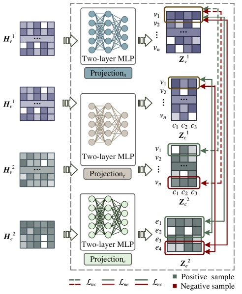
Figure 6: An example of cross-validation contrastive loss, where $V=\{v_{1},v_{2},\ldots,v_{n}\},E=\{e_{1},e_{2},e_{3},e_{4}\},E_{\{v_{1}\}}=\{e_{1},e_{2}\}$.

(iii) Hyperedge-cluster contrastive loss. This loss resembles the node-hyperedge contrastive loss in that the clustering result can be viewed as another mapping of node embeddings. If $v_{i}\in e_{j}$, the cluster results of $v_{i}$ and the embedding of $e_{j}$ are considered as a pair of positive samples; otherwise, they are designated as a pair of negative samples. Continuing the framework in Fig. 2, we calculate the loss between cluster results $\bm{Z}_{c}^{1}$ of $G_{1}$ and hyperedge embedding $\bm{Z}_{e}^{2}$ of $G_{2}$ (indicated by the solid arrows in Fig. 6), where $\bm{Z}_{c}^{1}$ and $\bm{Z}_{e}^{2}$ are projected from $\bm{H}_{v}^{1}$ and $\bm{H}_{e}^{2}$, respectively. Given $e_{1}=\{v_{1},v_{2}\}$ and $e_{2}=\{v_{1}\}$ (i.e. $E_{\{v_{1}\}}=\{e_{1},e_{2}\}$), $\bm{z}^{1}_{v,v_{1}}$ and $\bm{z}^{2}_{e,e_{1}}$ form a pair of positive samples, while $\bm{z}^{1}_{v,v_{1}}$ and $\bm{z}^{2}_{e,e_{4}}$ form a pair of negative samples. The hyperedge-cluster contrastive loss is defined as:

$$\mathcal{L}_{ec}=\frac{1}{2M}\sum_{v_{i}\in V}\sum_{e_{j}\in E_{\{v_{i}\}}}(\ell_{ec}(\bm{z}^{1}_{c,v_{i}},\bm{z}^{2}_{e,e_{j}})+\ell_{ec}(\bm{z}^{2}_{c,v_{i}},\bm{z}^{1}_{e,e_{j}})),$$ (17)

where $M=\sum_{v_{i}\in V}|E_{\{v_{i}\}}|$. The objective function $\ell_{ec}$ for hyperedge-cluster contrast is defined as:

$$\ell_{ec}(\bm{z}^{p}_{c,v_{i}},\bm{z}^{q}_{e,e_{j}})= -\log\frac{\exp(\mathcal{D}(\bm{z}^{p}_{c,v_{i}},\bm{z}^{q}_{e,e_{j}})/\tau_{ec})}{\sum_{v^{\prime}\in V}\exp(\mathcal{D}(\bm{z}^{p}_{c,v^{\prime}},\bm{z}^{q}_{e,e_{j}})/\tau_{ec})}$$ (18)

$$-\log\frac{\exp(\mathcal{D}(\bm{z}^{p}_{c,v_{i}},\bm{z}^{q}_{e,e_{j}})/\tau_{ec})}{\sum_{e^{\prime}\in E}\exp(\mathcal{D}(\bm{z}^{p}_{c,v_{i}},\bm{z}^{q}_{e,e^{\prime}})/\tau_{ec})},$$

where $p,q\in\{1,2\}$ and $\tau_{ec}$ is a temperature parameter corresponding to $\ell_{ec}$. Integrating Formulas 13, 15, and 17, the cross-validation contrastive loss becomes:

$$\mathcal{L}_{crocl}=\lambda_{nc}\mathcal{L}_{nc}+\lambda_{ne}\mathcal{L}_{ne}+\lambda_{ec}\mathcal{L}_{ec},\vspace{-1mm}$$ (19)

where $\lambda_{nc}$, $\lambda_{ne}$, and $\lambda_{ec}$ are positive hyperparameters that balance the importance of the three losses. Finally, the overall loss function of CHGNN is:

$$\mathcal{L}=\mathcal{L}_{sim}+\mathcal{L}_{cls}+\mathcal{L}_{h}+\mathcal{L}_{cl}+\mathcal{L}_{crocl},\vspace{-1mm}$$ (20)

where $\mathcal{L}_{sim}$ is the similarity loss from hypergraph view generators, $\mathcal{L}_{cls}$ is the classification loss, $\mathcal{L}_{h}$ is the hyperedge homogeneity loss, $\mathcal{L}_{cl}$ is the basic contrastive loss, and $\mathcal{L}_{crocl}$ is the cross-validation loss. We train CHGNN in an end-to-end manner. This (i) leads to classification-oriented view generators that sample the hypergraph to satisfy the InfoMin principle [18] and (ii) provides better-augmented views for CL.

4.5 Enhanced Contrastive Loss Training

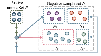
Figure 7: An example of enhanced contrastive loss training.

4.5.1 Adaptively Distancing Negative Samples

CL with the InfoNCE loss [40] typically requires a large number of negative samples to be effective, which is a practical challenge. Given the number of both clusters and classes $C$ (see Section 4.4.2), the number of negative samples for a training node is $C-1$ (see Section 4.4.2). We have $C<70$ for all of the nine datasets used in experiments (see Section 5), which implies a scarcity of negative samples in real-world scenarios. This hinders the efficient learning of feature information. To address this, we propose to identify negative samples that are difficult to distinguish from an instance (i.e., a target node cluster or a hyperedge) by applying a novel adaptive distancing method. The method effectively creates a “repulsion” between the negative samples and an instance, improving their separability and removing the necessity of training a large number of negative samples. This way, the proposed method can enable efficient and effective feature learning, even with few negative samples. We introduce the concept of relative penalty [41], before detailing the method.

Definition 9.

Given an instance $q$ and a set of negative samples $N=\{n_{1},n_{2},\ldots,n_{|N|}\}$, $\mathcal{R}=\{r_{n_{1}},r_{n_{2}},\ldots,r_{n_{|N|}}\}$ is a set of relative penalties, where $r_{n_{i}}$ is used to adjust the similarity between $q$ and nodes in $n_{i}$.

We use $s_{z}(q,n_{i})$ to denote the similarity between the embeddings of an instance $q$ and a negative sample $n_{i}$. According to the above discussion, it is desirable to impose a high $r_{n_{i}}$ on negative samples with a high $s_{z}(q,n_{i})$, in order to increase the embedding distances between nodes in $n_{i}$ and $q$ and thus to differentiate them.

Definition 10.

Given an instance $q$, a set of negative samples $N=\{n_{1},n_{2},\ldots,n_{|N|}\}$, and a set of relative penalties $\mathcal{R}=\{r_{n_{1}},r_{n_{2}},\ldots,r_{n_{|N|}}\}$, the desired ranking of relative penalties in $\mathcal{R}$ satisfies $\forall s_{z}(q,n_{i})>s_{z}(q,n_{j})\;(r_{n_{i}}>r_{n_{j}}),1\leq i,j\leq m$.

Example 5.

In Fig. 7, $P$ is a positive sample set, and $N$ is a negative sample set partitioned into non-overlapped subsets $N_{1}$, $N_{2}$, $N_{3}$, and $N_{4}$ ($N=N_{1}\cup N_{2}\cup N_{3}\cup N_{4}$). For simplicity, we assume that all negative samples in the same subset have the same embedding similarity to $q$, i.e., $s_{z}(q,n_{i})=s_{z}(q,n_{j})$, and we let $s_{z}(q,N_{k})=s_{z}(q,n_{i})\,(n_{i},n_{j}\in N_{k},1\leq k\leq 4)$, where $s_{z}(q,N_{k})$ denotes the similarity between $q$ and any $q^{\prime}\in N_{k}$. Then, we expect $r_{n_{i}}=r_{n_{j}}\,(n_{i},n_{j}\in N_{k},1\leq k\leq 4)$ (see Definition 9). We thus let $r_{N_{k}}=r_{n_{i}}$ $(n_{i}\in N_{k},1\leq k\leq 4)$. Next, given $s_{z}(q,N_{1})>s_{z}(q,N_{2})>s_{z}(q,N_{3})>s_{z}(q,N_{4})$, ideally we should have $r_{N_{1}}>r_{N_{2}}>r_{N_{3}}>r_{N_{4}}$.

The relative penalty $r_{n_{i}}$ associated with $n_{i}$ is [41]:

$$r_{n_{i}}=\left\lvert\frac{\partial\ell_{q}}{\partial s_{z}(q,n_{i})}\right\rvert\bigg{/}\left\lvert\frac{\partial\ell_{q}}{\partial s_{z}(q,p)}\right\rvert,$$ (21)

where $q$ is the training instance, $p$ and $n_{i}$ are positive and negative samples, $s_{z}(\cdot)$ is an embedding similarity function, $N$ is a negative sample set, and $\ell_{q}$ is the InfoNCE loss function of $q$ in each epoch:

$$\ell_{q}=-\log\frac{\mathcal{F}(q,p,\tau_{p})}{\mathcal{F}(q,p,\tau_{p})+\sum_{n_{i}\in N}\mathcal{F}(q,n_{i},\tau_{n})},$$ (22)

where $\mathcal{F}(a,b,c)=\exp(s_{z}(a,b)/c)$ and $\tau_{n}$ and $\tau_{p}$ are temperature hyperparameters that are fixed and set to the same value during normal contrastive loss training. The objective is to dynamically adjust the set of relative penalties $\mathcal{R}$ in order to satisfy the desired ranking (cf. Definitions 9 and 10). Formulas 21 and 22 suggest that the temperature hyperparameter $\tau_{n_{i}}$ uniquely determines $r_{n_{i}}$ for the negative sample $n_{i}$. This transfers the objective to the dynamic modification of temperature parameters for different negative samples during training.

Lemma 1.

Given a positive sample $p$, a training instance $q$, and a negative sample set $N=\{n_{1},n_{2}\}$ with $s_{z}(q,n_{1})>s_{z}(q,n_{2})$ then we have $r_{n_{1}}>r_{n_{2}}$ if $\tau_{n_{1}}=\tau^{ub}/s_{z}(q,n_{1})$ and $\tau_{n_{2}}=\tau^{ub}/s_{z}(q,n_{2})$, where $\tau^{ub}$ is the upper bound of the temperature parameter.

Proof.

According to Formulas 21 and 22:

$$r_{n_{1}}=\left\lvert\frac{\partial-\log\frac{\mathcal{F}(q,p,\tau_{p})}{\mathcal{F}(q,p,\tau_{p})+\sum_{n_{i}\in N}\mathcal{F}(q,n_{i},\tau_{n_{i}})}}{\partial s_{z}(q,n_{1})}\right\rvert\bigg{/}\left\lvert\frac{\partial\ell_{q}}{\partial s_{z}(q,p)}\right\rvert$$ (23)

Similarly, we have:

$$r_{n_{2}}=\left\lvert\frac{\partial-\log\frac{\mathcal{F}(q,p,\tau_{p})}{\mathcal{F}(q,p,\tau_{p})+\sum_{n_{i}\in N}\mathcal{F}(q,n_{i},\tau_{n_{i}})}}{\partial s_{z}(q,n_{2})}\right\rvert\bigg{/}\left\lvert\frac{\partial\ell_{q}}{\partial s_{z}(q,p)}\right\rvert.$$ (24)

Since Formulas 23 and 24 have the same denominator, proving $r_{n_{1}}>r_{n_{2}}$ is equivalent to proving:

$$\frac{\mathcal{F}(q,n_{1},\tau_{n_{1}})}{\mathcal{U}_{1}}>\frac{(\mathcal{F}(q,n_{2},\tau_{n_{2}})}{\mathcal{U}_{2}},$$ (25)

where $\mathcal{U}_{i}=\tau_{n_{i}}(\mathcal{F}(q,n_{1},\tau_{n_{1}})+\mathcal{F}(q,n_{2},\tau_{n_{2}})+\mathcal{F}(q,p,\tau_{p}))$ ($i=1,2$). Given $\tau_{n_{i}}=\tau^{ub}/s_{z}(q,n_{i})$, we have $\mathcal{F}(q,n_{i},\tau_{n_{i}})=\exp(s_{z}(q,n_{i})^{2}/\tau^{ub})$. Since $s_{z}(q,n_{1})>s_{z}(q,n_{2})$, $\tau_{n_{1}}<\tau_{n_{2}}$ and $\mathcal{F}(q,n_{1},\tau_{n_{1}})>\mathcal{F}(q,n_{2},\tau_{n_{2}})$. Thus, $r_{n_{1}}>r_{n_{2}}$ according to Formula 25. ∎

When $|N|>2$, $\tau_{n_{i}}=\tau^{ub}/s_{z}(q,n_{i})$ ($n_{i}\in N$) guarantees that $r_{n_{1}}>r_{n_{2}}>\ldots>r_{n_{|N|}}$ if $s_{z}(q,{n_{1}})>s_{z}(q,{n_{2}})>\ldots>s_{z}(q,{n_{|N|}})$. This can be derived straightforwardly.

4.5.2 Training Strategy

In Section 4.5.1, we detail the process and benefits of adaptively distancing negative samples. However, the representations of instances (i.e., node clusters or hyperedges) contain only poor feature information during the initial stages of training. Thus, we cannot start distancing two negative samples from each other before we have learned sufficient information for classification. This requires us to monitor the progress of the learning.

Differentiating cluster-level loss. If centers of different clusters (i.e., classes) are well separated, the cluster-level representations can capture rich feature information. Given a training set $V_{L}=\{V_{L}^{1},V_{L}^{2},\ldots,V_{L}^{C}\}$, where $C$ is the number of classes and $V_{L}^{i}$ includes the labeled nodes of class $c_{i}$, we calculate the embedding center $\bm{h}^{(k)}_{c_{i}}$ of cluster embddings $\bm{z}^{(k)}_{c,v_{\{i\}}}$ ($v_{\{i\}}\in V_{L}^{i}$) after $k$ epochs. Here, $\bm{z}^{(k)}_{c,v_{\{i\}}}=1/2(\bm{z}^{1,(k)}_{c,v_{\{i\}}}+\bm{z}^{2,(k)}_{c,v_{\{i\}}})$ and $(k)$ denotes the $k$-th epoch embeddings. We denote the similarities between centers $\bm{h}^{(k)}_{c_{i}}$ and $\bm{h}^{(k)}_{c_{j}}$ at the $k$-th epoch by $m_{ij}^{(k)}$. If $\overline{m}^{(k)}_{c}=\frac{1}{\binom{C}{2}}\sum_{(i,j)\in\binom{C}{2}}m_{ij}^{(k)}$ is below a threshold $\varepsilon_{c}$, we adjust the fixed temperature parameters $\tau_{c}$ of Formula 9. For each negative sample $c_{i}$ with anchor $c_{q}$ at the $k$-th epoch, the temperature parameter $\tau_{c,(q,i)}^{(k)}$ is defined as follows:

$$\tau_{c,(q,i)}^{(k)}=\begin{cases}\tau^{ub}_{c}&\text{if}\quad\overline{m}_{c}^{(k)}\geqslant\varepsilon_{c}\\ \tau^{ub}_{c}/s_{z}(\bm{Z}^{1,(k)}_{c:q},\bm{Z}^{2,(k)}_{c:i})&\text{otherwise}\end{cases},\vspace{-2mm}$$ (26)

where $\varepsilon_{c}$ is a threshold hyperparameter, $\tau_{c}^{ub}$ is the upper bound, and $\bm{Z}^{1,(k)}_{c:q}$ and $\bm{Z}^{2,(k)}_{c:i}$ are two cluster embedded representations at the $k$-th epoch.

Differentiating hyperedge-level contrastive loss. This procedure is similar to that of differentiating node-level contrastive loss. Since no class labels for hyperedges are available, we construct hyperedges with the training set $V_{L}$. All nodes in $V_{L}^{i}$ are assigned to a hyperedge $e_{V_{L}^{i}}$. Since a hyperedge describes a relationship among multiple nodes and $V_{L}^{i}$ includes the labeled nodes of class $c_{i}$, we assume that the constructed hyperedge $e_{V_{L}^{i}}$ belongs to class $c_{i}$. If the distributions of the constructed hyperedge representations differ from each other, the representation of the hyperedge is rich in feature information. Thus, when the mean $\overline{m}_{e}^{(k)}$ of the similarities between hyperedge representations is below a threshold $\varepsilon_{e}$ at the $k$-th epoch, we adjust the temperature parameters $\tau_{e}$ of Formula 11. For each negative sample $e_{i}$ with anchor $e_{q}$ at the $k$-th epoch, the temperature parameter $\tau_{e,(q,i)}^{(k)}$ is defined as follows:

$$\tau_{e,(q,i)}^{(k)}=\begin{cases}\tau_{e}^{ub}&\text{if}\quad\overline{m}_{e}^{(k)}\geqslant\varepsilon_{e}\\ \tau_{e}/s_{z}(\bm{Z}^{1}_{e,e_{q}},\bm{Z}^{2}_{e,e_{i}})&\text{otherwise}\end{cases},\vspace{-1mm}$$ (27)

where $\varepsilon_{e}$ is a threshold hyperparameter, $\tau_{e}^{ub}$ is the upper bound, and $\bm{Z}^{1,(k)}_{e,e_{q}}$ and $\bm{Z}^{2,(k)}_{e,e_{i}}$ are two hyperedge embedded representations at the $k$-th epoch.

TABLE I: Hypergraphs statistics from the nine datasets.

Dataset	#nodes	#hyperedges	#attributes	#classes
CA-Cora	2,708	1,072	1,433	7
CA-DBLP	43,413	22,535	1425	6
Cora	2,708	1,579	1,433	7
Citeseer	3,312	1,079	3,703	6
Pubmed	19,717	7,963	500	3
20news	16,242	100	100	4
ModelNet	12,311	12,311	100	40
NTU	2,012	2,012	100	67
Mushroom	8,124	298	22	2

TABLE II: Hyperparamter settings for CHGNN.

Dataset	$\bm{\lambda_{e}}$	$\bm{\lambda_{nc}}$	$\bm{\lambda_{ne}}$	$\bm{\lambda_{ec}}$	nhid	nproj
CA-Cora	0.2	0.2	0.2	0.2	64	16
CA-DBLP	0.0625	0	0.25	0.25	64	16
Pubmed	0.9	0.8	0.7	0.7	64	16
Citeseer	0.8	1	0.8	0.8	64	16
Cora	0.7	0.5	0.9	0.9	64	16
20news	0.1	0.8	0.6	0.6	64	16
ModelNet	0.7	0.1	0.032	0	256	16
NTU	0.3	0.1	0.7	0.7	512	512
Mushroom	0.2	0	0.1	0.024	64	16

TABLE III: Comparison results (%), where (i) $*$ denotes unsupervised learning methods, (ii) the results in bold denote the best performance and those underlined denote the second best performance, and (iii) OOM denotes out of memory on a 24GB GPU.

	Dataset	CA-Cora	CA-DBLP	Pubmed	Citeseer	Cora	20news	ModelNet	NTU	Mushroom
	MLP	59.2 $\pm$ 1.2	79.5 $\pm$ 0.4	71.8 $\pm$ 1.4	58.8 $\pm$ 1.2	59.3 $\pm$ 1.1	64.9 $\pm$ 2.0	93.7 $\pm$ 0.3	75.4 $\pm$ 1.5	89.2 $\pm$ 2.6
Graph	GCN	65.3 $\pm$ 1.5	84.6 $\pm$ 0.3	72.0 $\pm$ 2.0	59.2 $\pm$ 1.3	62.6 $\pm$ 2.3	71.1 $\pm$ 2.2	93.6 $\pm$ 0.3	74.8 $\pm$ 2.0	87.8 $\pm$ 1.4
	GAT	63.1 $\pm$ 2.0	84.6 $\pm$ 0.3	70.4 $\pm$ 2.9	59.0 $\pm$ 1.2	62.5 $\pm$ 1.5	73.8 $\pm$ 3.1	94.1 $\pm$ 0.2	72.6 $\pm$ 1.7	86.8 $\pm$ 3.0
	DGI∗	64.1 $\pm$ 0.2	78.5 $\pm$ 0.2	67.9 $\pm$ 0.1	51.3 $\pm$ 0.1	61.3 $\pm$ 0.2	75.8 $\pm$ 0.1	95.8 $\pm$ 0.1	77.8 $\pm$ 0.2	85.3 $\pm$ 0.0
	SimGRACE∗	64.1 $\pm$ 0.4	78.8 $\pm$ 0.2	69.8 $\pm$ 0.0	53.3 $\pm$ 0.1	61.2 $\pm$ 0.3	76.1$\pm$0.1	95.0 $\pm$ 0.1	77.7 $\pm$ 0.2	86.7 $\pm$ 0.2
Hypergraph	HyperConv	65.9 $\pm$ 0.8	88.2 $\pm$ 0.1	39.4 $\pm$ 7.6	37.3 $\pm$ 3.3	44.6 $\pm$ 4.1	75.9 $\pm$ 1.1	91.9 $\pm$ 0.1	78.2 $\pm$ 0.8	94.8 $\pm$ 1.9
	HGNN	71.7 $\pm$ 1.0	70.2 $\pm$ 2.1	72.8 $\pm$ 1.2	60.8 $\pm$ 1.0	67.2 $\pm$ 1.2	75.1 $\pm$ 1.7	93.7 $\pm$ 0.2	75.7 $\pm$ 1.7	92.6 $\pm$ 1.9
	HyperGCN	72.6 $\pm$ 8.7	87.9 $\pm$ 1.5	72.0 $\pm$ 10.2	59.7 $\pm$ 9.3	66.1 $\pm$ 6.7	68.3 $\pm$ 1.0	93.0 $\pm$ 4.7	68.1 $\pm$ 5.1	92.4 $\pm$ 0.4
	HNHN	66.5 $\pm$ 6.9	86.8 $\pm$ 0.3	69.2 $\pm$ 5.3	55.2 $\pm$ 3.4	62.9 $\pm$ 3.3	71.6 $\pm$ 1.6	94.4 $\pm$ 0.4	72.3 $\pm$ 1.9	90.6 $\pm$ 2.7
	HyperSAGE	73.1 $\pm$ 1.5	87.0 $\pm$ 0.2	73.0 $\pm$ 1.7	61.8 $\pm$ 1.4	67.3 $\pm$ 1.6	73.8 $\pm$ 1.8	92.8 $\pm$ 1.0	72.5 $\pm$ 0.5	92.9 $\pm$ 2.3
	UniGNN	74.0 $\pm$ 1.2	88.5 $\pm$ 0.1	74.5 $\pm$ 1.6	62.7$\pm$ 1.8	68.4 $\pm$ 2.4	75.1 $\pm$ 2.0	96.4 $\pm$ 0.2	81.2$\pm$ 1.7	93.5 $\pm$ 3.0
	AST	71.5 $\pm$ 1.9	87.0 $\pm$ 0.6	54.5 $\pm$ 10.3	60.0 $\pm$ 3.4	64.6 $\pm$ 2.7	73.3 $\pm$ 1.1	93.0 $\pm$ 0.4	81.0 $\pm$ 2.9	93.3 $\pm$ 2.5
	TriCL∗	77.3 $\pm$ 0.7	OOM	75.6 $\pm$ 1.6	66.1 $\pm$ 1.1	74.9 $\pm$ 1.0	76.8 $\pm$ 0.8	96.6 $\pm$ 0.1	81.9 $\pm$ 1.5	94.3 $\pm$ 1.7
	CHGNN	78.5 $\pm$ 1.0	89.2 $\pm$ 0.2	78.4 $\pm$ 0.8	69.4 $\pm$ 1.6	75.7 $\pm$ 0.6	77.5 $\pm$ 0.9	96.8 $\pm$ 0.1	83.7 $\pm$ 0.7	95.0 $\pm$ 1.0

5 Experimental Study

5.1 Experimental Setup

5.1.1 Datasets

We evaluate CHGNN using nine public real datasets. Table I summarizes statistics of their hypergraphs.

Cora. We construct a citation hypergraph, where each node represents a paper and each hyperedge contains all publications of the same paper. The construction of this and the next four datasets follow [2, 23, 11].

CA-Cora. We construct a coauthorship hypergraph, where each node represents a publication and each hyperedge contains all publications by the same author.

CA-DBLP. We construct a coauthorship hypergraph, where each node represents a paper and each hyperedge contains all publications by the same author.

Pubmed¹. We construct a citation hypergraph, where each node represents a paper and each hyperedge contains all publications cited by the same paper.

Citeseer¹. We construct a citation hypergraph, where each node represents a paper and each hyperedge contains all publications cited by the paper.

20news. We construct a news-word hypergraph, where each node represents a piece of news and each hyperedge represents all news that contain the same word. The construction of this and the next three datasets follows [22].

Mushroom⁴. We construct a mushroom-feature hypergraph, where each node represents a mushroom and each hyperedge contains all data with the same categorical features.

ModelNet. We construct a nearest-neighbor hypergraph, where each node represents a CAD model and each hyperedge is constructed by Multi-view Convolutional Neural Network (MVCNN) features with ten nearest neighbors.

NTU [42]. We construct a nearest-neighbor hypergraph, where each node represents a shape and each hyperedge is constructed by MVCNN features with ten nearest neighbors.

5.1.2 Competitors

We compare CHGNN with thirteen state-of-the-art proposals.

MLP [43] is a supervised learning framework that primarily focuses on encoding the features of node attributes without considering the underlying graph structure.

GCN [8] is a semi-supervised learning framework that employs a convolutional neural network architecture to perform node classification tasks on graphs.

GAT [44] utilizes a multi-head attention mechanism to dynamically generate aggregated weights for neighboring nodes.

DGI [13] is an unsupervised graph representation learning framework that maximizes the mutual information between node representations and high-level summaries of the graph structure.

SimGRACE [35] is a GCL model that generates graph views by model parameter perturbation.

HyperConv[20] is a graph representation learning framework that leverages higher-order relationships and local clustering structures for representation learning.

HGNN [1] is a graph representation learning model that generalizes and then approximates the convolution operation using truncated Chebyshev polynomials to enhance representation learning.

HyperGCN [2] is a semi-supervised learning framework based on spectral theory.

HNHN [24] is a HyperGCN with nonlinear activation functions combined with a normalization scheme that can flexibly adjust the importance of hyperedges and nodes.

HyperSAGE [23] is a graph representation learning framework that learns to embed hypergraphs by aggregating messages in a two-stage procedure.

UniGNN [11] is a unified framework for interpreting the message-passing process in hypergraph neural networks. We report the results of UniSAGE, a variant of UniGNN that achieves the best average performance among all the variants in most cases [11].

AST [22] is the state-of-the-art supervised hypergraph-based model, which propagates information by a multiset function learned by Deep Sets [45] and Set Transformer [46].

TriCL [15] is a state-of-the-art unsupervised contrastive hypergraph learning model that maximizes the mutual information between nodes, hyperedges, and groups.

MLP is a feature-based model, while GCN, GAT, DGI, and SimGRACE are graph-based models. The remaining baselines are hypergraph-based models. To enable the comparison of graph-based models with hypergraphs, we project hypergraphs to 2-projected graphs [47]. Since unsupervised learning models have shown comparable performance to supervised learning models [31, 35, 15], we compare CHGNN with three state-of-the-art unsupervised models: DGI, SimGRACE, and TriCL.

5.1.3 Hyperparameters and Experimental Settings

We use 20 labeled nodes per class in all datasets (except NTU) for training and use the remaining nodes for testing. For NTU, we use 10% of the nodes for training and the remaining nodes for testing. This is because NTU has relatively many categories (67) but few nodes (2012), yielding an excessive label ratio. Following existing studies [22, 1, 2, 23, 11], we validate the performance of CHGNN and all baselines by performing classification and report the average node classification accuracy. In particular, 10-fold cross-validation is conducted on each dataset.

We set the hyperparameters of the baselines as suggested by the respective papers. For CHGNN, we set the number of layers in the H-HyperGNN to 2 and use an MLP consisting of two fully connected layers with 16 neurons in the hidden layer. For the node classification task, we set $p_{node}=0.2$, $p_{\tau}=0.8$, $\varepsilon_{c}=0.2$, $\varepsilon_{e}=0.2$, $\lambda_{h}=1$, and $\lambda_{c}=1$. Other hyperparameters are listed in Table II where nhid is the embedding dimensionality of the hidden layer and nproj is the projection dimensionality. The source code is available online. All experiments are conducted on a server with an Intel(R) Xeon(R) W-2155 CPU, 128GB memory, and an NVIDIA TITAN RTX GPU.

TABLE IV: Classification accuracy with different label ratio (%) on Cora.

Label Ratio	0.5%	1%	2%	3%	10%	20%	30%	40%	50%
MLP	31.1 $\pm$ 3.2	39.9 $\pm$ 4.7	45.7 $\pm$ 4.7	52.6 $\pm$ 1.8	63.8 $\pm$ 1.8	68.5 $\pm$ 0.6	70.5 $\pm$ 0.9	72.7 $\pm$ 1.1	73.2 $\pm$ 0.9
GCN	21.3 $\pm$ 6.5	36.7 $\pm$ 8.2	47.2 $\pm$ 3.6	53.5 $\pm$ 4.4	66.4 $\pm$ 1.4	69.7 $\pm$ 1.0	72.0 $\pm$ 1.0	73.2 $\pm$ 0.8	74.3 $\pm$ 1.1
GAT	24.8 $\pm$ 7.0	39.4 $\pm$ 2.3	49.0 $\pm$ 3.8	53.4 $\pm$ 2.9	66.0 $\pm$ 0.7	70.9 $\pm$ 0.5	72.1 $\pm$ 1.0	73.0 $\pm$ 0.9	74.3 $\pm$ 0.5
DGI	26.8 $\pm$ 0.4	30.2 $\pm$ 0.2	38.8 $\pm$ 0.5	43.3 $\pm$ 0.5	62.0 $\pm$ 0.3	63.8 $\pm$ 0.3	63.6 $\pm$ 0.3	63.2 $\pm$ 0.3	62.3 $\pm$ 0.4
SimGRACE	24.9 $\pm$ 0.7	31.4 $\pm$ 3.7	37.1 $\pm$ 1.8	41.4 $\pm$ 1.5	62.9 $\pm$ 1.1	62.1 $\pm$ 0.6	61.8 $\pm$ 0.5	62.6 $\pm$ 0.7	62.7 $\pm$ 1.0
HyperConv	27.2 $\pm$ 3.3	30.8 $\pm$ 5.3	36.6 $\pm$ 3.4	43.2 $\pm$ 6.0	50.0 $\pm$ 5.2	55.9 $\pm$ 5.1	54.2 $\pm$ 7.8	62.5 $\pm$ 0.7	66.1 $\pm$ 0.5
HGNN	30.2 $\pm$ 9.0	40.8 $\pm$ 8.8	56.7 $\pm$ 3.8	60.4 $\pm$ 3.3	71.6 $\pm$ 0.8	75.8 $\pm$ 0.8	77.1 $\pm$ 1.0	77.3 $\pm$ 1.0	78.6 $\pm$ 1.7
HyperGCN	35.2 $\pm$ 8.4	36.1 $\pm$ 11.7	50.6 $\pm$ 4.3	58.8 $\pm$ 2.6	69.6 $\pm$ 2.0	73.5 $\pm$ 0.9	74.4 $\pm$ 0.8	74.6 $\pm$ 5.2	75.9 $\pm$ 4.9
HNHN	31.7 $\pm$ 5.5	44.9 $\pm$ 8.4	52.6 $\pm$ 5.7	56.2 $\pm$ 1.1	68.0 $\pm$ 0.6	71.1 $\pm$ 1.0	72.6 $\pm$ 1.4	74.6 $\pm$ 3.1	74.9 $\pm$ 1.6
HyperSAGE	39.9 $\pm$ 3.7	47.0 $\pm$ 4.3	54.9 $\pm$ 1.1	58.4 $\pm$ 1.6	68.9 $\pm$ 1.9	73.4 $\pm$ 1.2	76.4 $\pm$ 0.8	77.0 $\pm$ 0.9	77.7 $\pm$ 1.0
UniGNN	38.5 $\pm$ 4.4	49.0 $\pm$ 5.1	58.5 $\pm$ 3.2	62.5 $\pm$ 1.0	71.7 $\pm$ 1.6	74.5 $\pm$ 1.0	76.8 $\pm$ 0.7	77.1 $\pm$ 0.6	78.4 $\pm$ 1.0
AST	48.6 $\pm$ 4.6	49.8 $\pm$ 2.3	55.5 $\pm$ 3.9	58.9 $\pm$ 1.2	69.5 $\pm$ 1.0	71.4 $\pm$ 0.8	75.2 $\pm$ 0.2	77.9 $\pm$ 3.2	78.4 $\pm$ 1.2
TriCL	53.3 $\pm$ 7.5	66.7 $\pm$ 4.2	69.8 $\pm$ 3.4	73.5 $\pm$ 2.1	76.9 $\pm$ 0.6	78.6 $\pm$ 0.7	78.2 $\pm$ 0.5	78.5 $\pm$ 0.7	79.0 $\pm$ 0.8
CHGNN	64.8 $\pm$ 5.6	66.6 $\pm$ 2.2	72.2 $\pm$ 2.1	73.9 $\pm$ 2.0	76.9 $\pm$ 0.6	78.7 $\pm$ 0.2	78.5 $\pm$ 0.1	79.7 $\pm$ 1.1	79.9 $\pm$ 0.3

TABLE V: Ablation results.

$\bm{L}_{h}$	$\bm{L}_{cl}$	$\bm{L}_{crocl}$	Aug	Encoder	CA-Cora	CA-DBLP	Pubmed	Citeseer	Cora
-	-	-	-	HyperGNN	74.0 $\pm$ 0.4	87.9 $\pm$ 0.1	75.1 $\pm$ 0.8	62.0 $\pm$ 0.8	66.8 $\pm$ 1.5
✓	-	-	-	HyperGNN	73.1 $\pm$ 0.7	87.1 $\pm$ 0.1	74.9 $\pm$ 0.3	60.3 $\pm$ 0.7	64.8 $\pm$ 1.3
-	-	-	-	H-HyperGNN	74.5 $\pm$ 0.1	88.1 $\pm$ 0.1	75.4 $\pm$ 0.9	61.6 $\pm$ 1.3	67.3 $\pm$ 1.3
✓	-	-	-	H-HyperGNN	74.7 $\pm$ 0.1	88.2 $\pm$ 0.1	75.9 $\pm$ 1.1	62.5 $\pm$ 0.2	67.4 $\pm$ 1.2
-	✓	-	RandAug	HyperGNN	71.8 $\pm$ 1.6	88.5 $\pm$ 0.2	74.6 $\pm$ 1.6	59.1 $\pm$ 3.2	63.1 $\pm$ 2.6
-	-	✓	RandAug	HyperGNN	75.5 $\pm$ 0.8	88.7 $\pm$ 0.2	75.8 $\pm$ 3.6	68.2 $\pm$ 1.7	72.0 $\pm$ 1.6
-	✓	✓	RandAug	HyperGNN	74.0 $\pm$ 0.9	88.6 $\pm$ 0.2	75.4 $\pm$ 4.0	67.7 $\pm$ 1.1	70.5 $\pm$ 2.2
✓	✓	-	RandAug	H-HyperGNN	70.3 $\pm$ 2.3	88.6 $\pm$ 0.2	74.1 $\pm$ 1.7	58.9 $\pm$ 1.9	63.7 $\pm$ 1.3
✓	-	✓	RandAug	H-HyperGNN	75.3 $\pm$ 1.2	88.8 $\pm$ 0.2	76.7 $\pm$ 3.4	67.5 $\pm$ 1.5	71.5 $\pm$ 0.6
✓	✓	✓	RandAug	H-HyperGNN	74.5 $\pm$ 1.9	88.5 $\pm$ 0.3	76.1 $\pm$ 2.6	67.0 $\pm$ 2.3	69.9 $\pm$ 3.8
-	✓	-	ViewGen	HyperGNN	75.7 $\pm$ 1.0	89.2 $\pm$ 0.1	75.5 $\pm$ 1.5	62.6 $\pm$ 1.5	66.3 $\pm$ 2.6
-	-	✓	ViewGen	HyperGNN	76.5 $\pm$ 1.3	89.1 $\pm$ 0.2	77.9 $\pm$ 1.7	67.6 $\pm$ 1.8	73.1 $\pm$ 0.9
-	✓	✓	ViewGen	HyperGNN	76.8 $\pm$ 1.4	89.1 $\pm$ 0.1	77.7 $\pm$ 1.8	67.9 $\pm$ 1.2	72.6 $\pm$ 1.3
✓	✓	-	ViewGen	H-HyperGNN	78.1 $\pm$ 1.2	89.1 $\pm$ 0.2	75.3 $\pm$ 1.3	62.1 $\pm$ 1.2	71.0 $\pm$ 2.4
✓	-	✓	ViewGen	H-HyperGNN	77.5 $\pm$ 1.0	89.1 $\pm$ 0.2	76.4 $\pm$ 1.0	68.0 $\pm$ 1.8	74.3 $\pm$ 0.7
✓	✓	✓	ViewGen	H-HyperGNN	78.3 $\pm$ 1.0	89.3 $\pm$ 0.2	78.3 $\pm$ 2.9	68.5 $\pm$ 1.7	75.5 $\pm$ 0.9

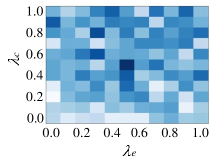
(a) Impact of $\lambda_{c}$ and $\lambda_{e}$ (Cora)

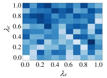
(b) Impact of $\lambda_{c}$ and $\lambda_{e}$ (Citeseer)

(c) Impact of $\varepsilon_{c}$ and $\varepsilon_{e}$ (Cora)

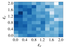
(d) Impact of $\varepsilon_{c}$ and $\varepsilon_{e}$ (Citeseer)

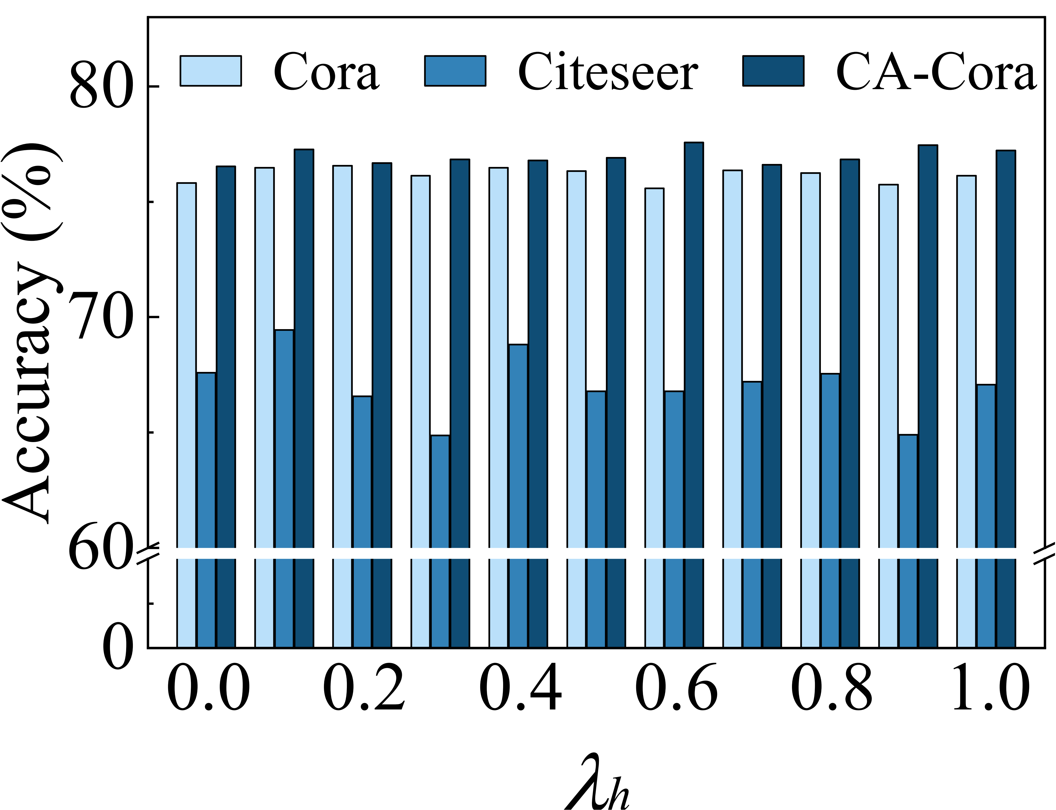
(e) Impact of $\lambda_{h}$

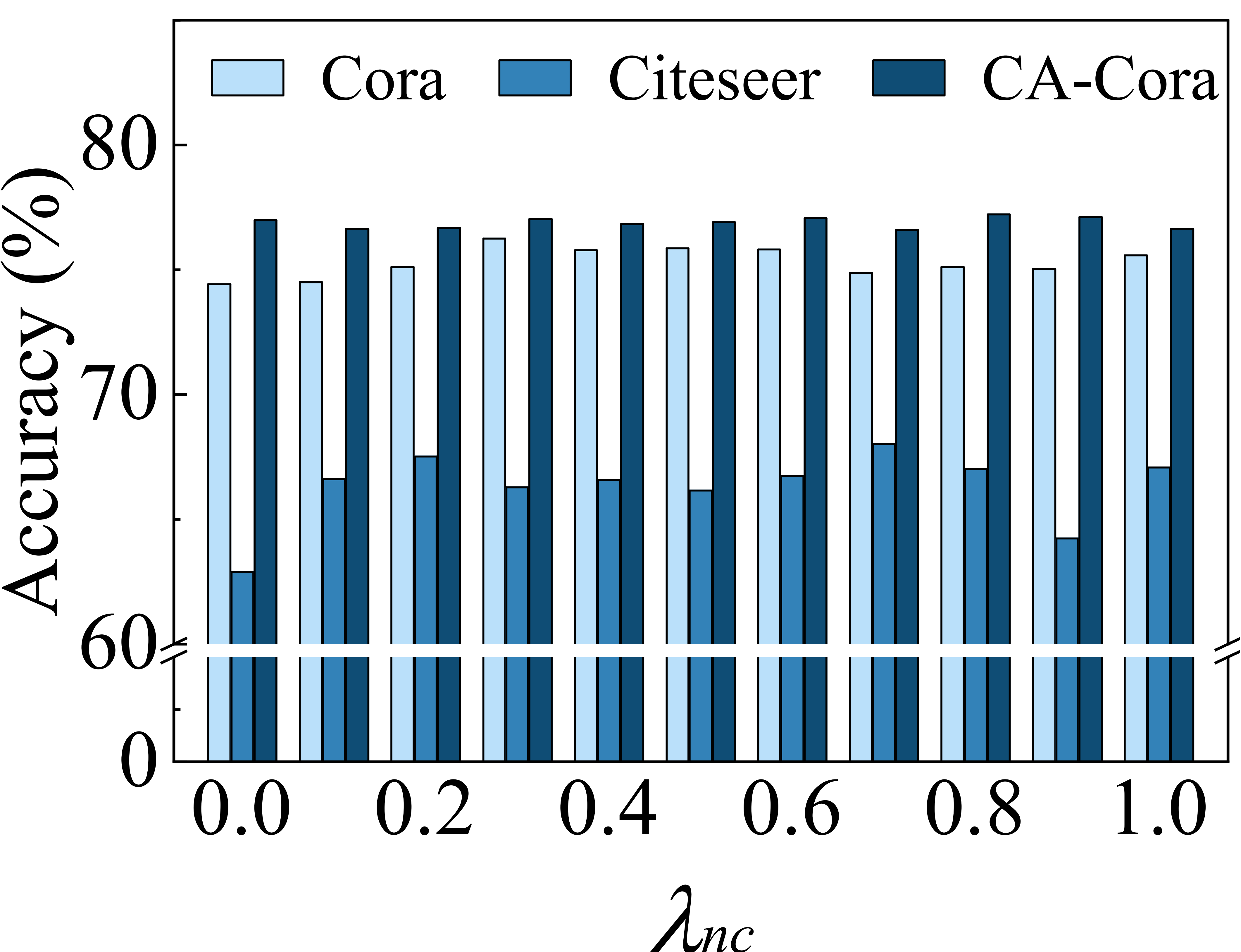
(f) Impact of $\lambda_{nc}$

(g) Impact of $\lambda_{ne}$

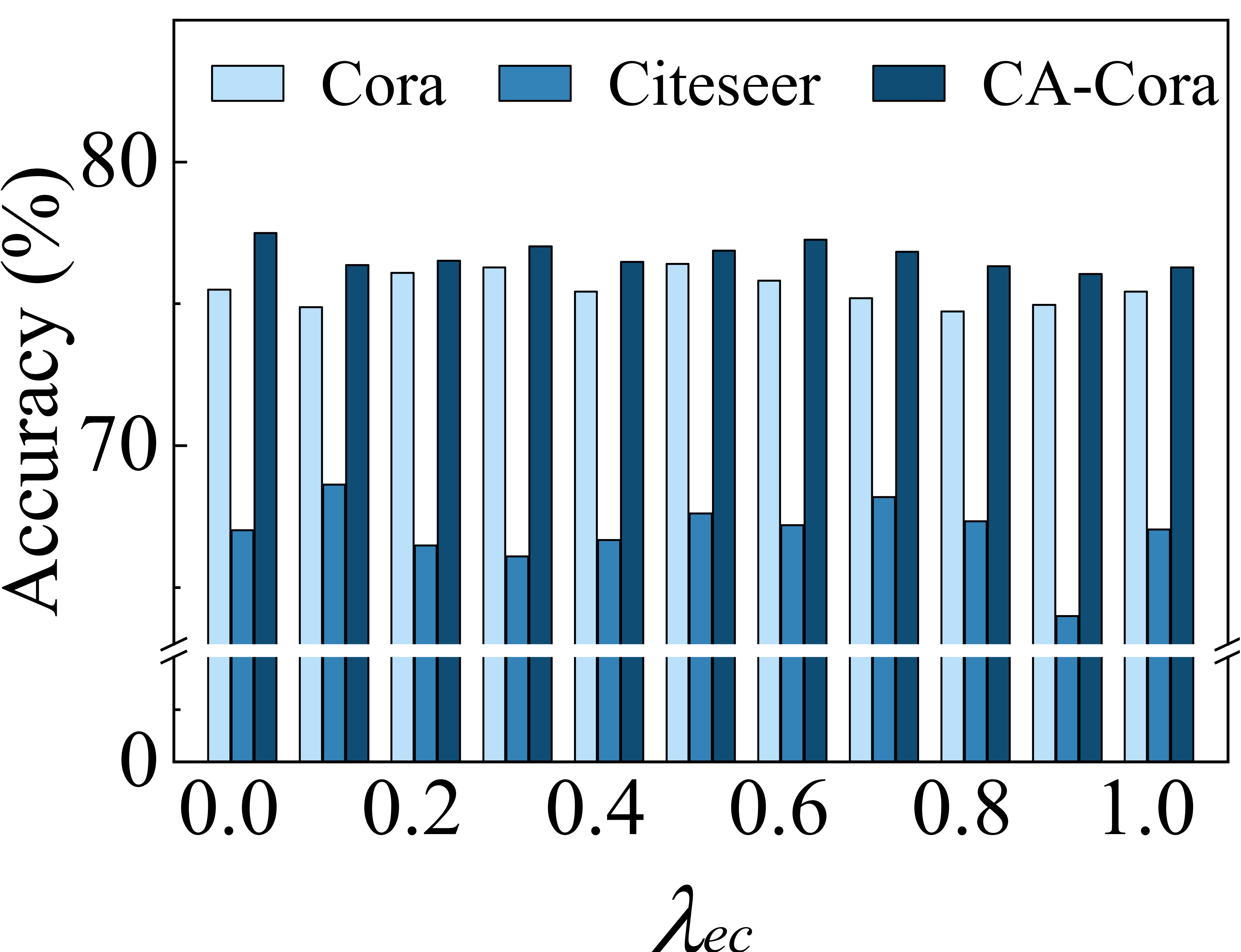
(h) Impact of $\lambda_{ec}$

Figure 8: Impact of hyperparameters.

5.2 Comparison

Table III summarizes the accuracy of all methods. CHGNN achieves consistently the highest accuracy on all datasets, outperforming the best competitors by 1.6% on CA-Cora, 0.7% on CA-DBLP, 3.7% on Pubmed, 4.9% on Citeseer, 1% on Cora, 0.9% on 20news, 0.2% on ModelNet, 2.1% on NTU, and 0.2% on Mushroom. This demonstrates the improved learning capability and robustness of CHGNN. Moreover, there are three notable observations as follows.

First, feature-based method MLP, while effective at learning from data with clear feature structures, does not consider the structural information of a hypergraph. Next, the graph-based methods GCN, GAT, DGI, and SimGRACE require the conversion of hypergraphs into graphs, which results in the loss of structural information, making them less effective. HyperGNNs, however, are able to learn richer information from hypergraphs by directly incorporating the structural information into the learning process, leading to more effective and accurate learning outcomes.

Second, TriCL performs comparably to all supervised baselines, even without any labeled data. TriCL outperforms the state-of-the-art AST and UniGNN on CA-Cora, Pubmed, Citeseer, Cora, 20news, ModelNet, and NTU. This indicates that CL captures potential information from unlabeled nodes effectively. Compared with TriCL, CHGNN (i) incorporates contrastive loss in training to enhance supervised learning and (ii) provides enough variance for CL via the view generator.

Third, although AST can perform well with sufficient training data (e.g., 50% labeled data [22]), it is not well-suited to our target application scenario with limited labeled data. In contrast, CHGNN requires relatively little labeled data to achieve high learning performance. This is due in part to its use of CL, which can capture the information from unlabeled data effectively.

5.3 Effect of Label Ratios

We evaluate the classification accuracy of CHGNN and the competitors, where 0.5%, 1%, 2%, 3%, 10%, 20%, 30%, 40%, and 50% of the nodes are labeled. Table IV show the results on Cora. CHGNN improves on the competitors in all settings. The performance of CHGNN trained by 3% labeled nodes is comparable to that of UniGNN trained by 10%. In sparse training data scenarios, e.g., when only 0.5% of the nodes are labeled, CHGNN’s advantage against the best competitor TriCL is 21.5%. Moreover, CHGNN outperforms the best semi-supervised competitor AST by 1.9%, even when 50% of the nodes are labeled. We attribute this to the CL component of CHGNN, which mines topological and feature information through constructed positive and negative samples and enables it to learn better from unlabeled data. Results on the remaining seven datasets show similar patterns.

Next, the classification accuracy of the semi-supervised methods increases linearly with the label ratio, while the performance of the CL methods becomes stable when the label ratio exceeds 20%. This is because CL methods ignore supervised information during training. The node embedding distribution generated by CL does not match well the distribution of the labels. Thus, it is difficult for the downstream classifier to accurately identify class boundaries based on the training set. In addition, CHGNN outperforms the semi-supervised competitors, due to its use of contrastive loss for embedding learning.

5.4 Parameter Analysis

Effect of $\lambda_{c}$ and $\lambda_{e}$. We evaluate the impact of $\lambda_{c}$ and $\lambda_{e}$ on classification, where $\lambda_{c}$ and $\lambda_{e}$ control the basic contrastive losses (see Section 4.4.2). Figs. 8 (a) and (b) are heatmaps showing classification accuracy on Cora and Citeseer, respectively, where both $\lambda_{c}$ and $\lambda_{e}$ are varied from 0 to 1. Darker grids in the figures indicate higher accuracy. CHGNN achieves the highest accuracy when $0.2<\lambda_{c}<0.6$ and $0.4<\lambda_{e}<0.6$ on Cora, and it performs well when $\lambda_{c}>0.6$ and $\lambda_{e}<0.9$ on Citeseer. This is because the labeled node ratio is 3.6% for Citeseer, which is smaller than that of in Cora (5.2%), so CHGNN requires more unlabeled information when training for the Citeseer dataset compared to Cora.

Effect of $\varepsilon_{c}$ and $\varepsilon_{e}$. We evaluate the impact of $\varepsilon_{c}$ and $\varepsilon_{e}$ on classification, where $\varepsilon_{c}$ and $\varepsilon_{e}$ determine the timing of the adaptive adjustment of repulsion (see Section  4.5.2). Figs. 8 (c) and (d) report the results on Cora and Citeseer, respectively, with both $\varepsilon_{c}$ and $\varepsilon_{e}$ being varied from 0 to 2. Darker grids indicate higher accuracy. When $\varepsilon_{c}$ and $\varepsilon_{e}$ are set to 0, the model pushes similar nodes apart, which can result in lower classification performance. When $\varepsilon_{c}$ and $\varepsilon_{e}$ are both larger than 1, the training performance of CHGNN degrades as there is almost no adjusted repulsion. The best performance is achieved for $0.6<\varepsilon_{c}<1.6$ and $0.2<\varepsilon_{e}<0.6$ on both datasets. This is because there are significantly fewer clusters than hyperedges that contain higher-order relationships in Cora and Citeseer. Only when the similarity of the embeddings of the constructed hyperedges is sufficiently small, we can ensure that the model can correctly adjust the adaptive repulsion by similarity.

Effect of $\lambda_{h}$, $\lambda_{nc}$, $\lambda_{ne}$, and $\lambda_{ec}$. We evaluate the impact of $\lambda_{h}$, $\lambda_{nc}$, $\lambda_{ne}$, and $\lambda_{ec}$ on classification, where $\lambda_{h}$ controls the hyperedge homogeneity loss (see Section 4.4.1) and $\lambda_{nc}$, $\lambda_{ne}$, and $\lambda_{ec}$ control the cross-validation contrastive losses (see Section 4.4.2). Figs. 8 (e) – (h) report the results on Cora, Citeseer, and CA-Cora, respectively, with $\lambda_{h}$, $\lambda_{nc}$, $\lambda_{ne}$, and $\lambda_{ec}$ being varied from 0 to 1. For $\lambda_{h}$, CHGNN performs the best when $0<\lambda_{h}<0.2$. Although the loss avoids nodes aggregating too much heterogeneous information, the distributions of hyperedge homogeneity and categories are not exactly the same. For $\lambda_{nc}$, CHGNN underperforms when $\lambda_{nc}=0$. In particular, cross-validation between nodes and clusters allows nodes to learn clustering information while maintaining their own features. CHGNN performs the best when $0.1<\lambda_{nc}<0.7$. This is because an excessive weight can weaken the difference between the node and cluster embeddings and disturb the embedding distribution of the nodes or clusters. For $\lambda_{ne}$, we see that when $\lambda_{ne}<0.5$, the node embedding ignores some of the higher-order information in the hyperedges, resulting in lower accuracy. When $0.5<\lambda_{ne}<1$, CHGNN corrects the node embedding distribution using cross-validation between nodes and hyperedges, thus improving the performance. For $\lambda_{ec}$, CHGNN performs the best when $0<\lambda_{ec}<0.2$, which is attributed to the difference between the distribution of node cluster embeddings and the hyperedge embeddings caused by the hyperedge homogeneity.

5.5 Ablation Study

We present an ablation study on CA-Cora, CA-DBLP, Pubmed, Citeseer, and Cora. Table V shows the results. $L_{h}$, $L_{cl}$, and $L_{crocl}$ represent hyperedge homogeneity loss, basic contrastive losses, and cross-validation contrastive loss, respectively. "Aug" indicates the strategy of augmenting the views, which can be no CL (represented by "-"), RandAug, and ViewGen. RandAug generates views by randomly removing 20% of the hyperedges [15]. ViewGen is the proposed adaptive hypergraph view generator embedded in CHGNN. "Encoder" indicates the model used for encoding hypergraphs, which can be HyperGNN and H-HyperGNN. HyperGNN is a common hypergraph encoder without homogeneity encoding [1]. H-HyperGNN is the hyperedge homogeneity-aware HyperGNN encoding model (see Formula 5) in CHGNN.

The results show that the three losses $L_{h}$, $L_{cl}$, and $L_{crocl}$, and view generator "ViewGen" and hypergraph encoder "H-HyperGCNN" contribute significantly to the performance of CHGNN. In particular, (i) the accuracy of H-HyperGNN is increased by 0.3 – 0.5% over HyperGNN; (ii) the accuracy of $L_{h}$ + H-HyperGNN is increased by 0.1 – 0.9% over H-HyperGNN; and (iii) the accuracy of CHGNN is increased by 1.1 – 8.1% over $L_{h}$ + H-HyperGNN.

Second, the proposed $L_{h}$ is not suitable for HyperGNN, as the accuracy of $L_{h}$ + HyperGNN drops by 0.2 – 2%. Specifically, HyperGNN does not consider homogeneity during aggregation, making it impossible to fit the distribution of the hyperedge homogeneity. Finally, when generating views by random augmentation (i.e., RandAug), adopting cross-validation contrastive losses (i.e., $L_{crocl}$) yields better performance than when adopting joint contrastive loss (i.e., $L_{cl}$ + $L_{crocl}$). This is because random sampling misses critical information, which hurts the clustering performance of nodes. Thus, nodes of different classes are grouped into a cluster, which reduces the training performance of the cluster-level contrastive loss. The same applies to the hyperedge-level contrastive loss. However, the cross-validation contrastive losses can work properly because they compare the same nodes with the clusters or hyperedges they belong to.

5.6 Study of the Enhanced Training Strategy

Fig. 9 reports the classification accuracy with and without the proposed enhanced training strategy (see Section 4.5), denoted as CHGNN and CHGNN (w/o T), on Cora and Citeseer, respectively. Clearly, the accuracy of CHGNN is higher than that of CHGNN (w/o T) on both datasets. For Cora, CHGNN (w/o T) converges at around the 180-th epoch and CHGNN converges at around the 200-th epoch. The adaptive distance adjustment starts at the 85-th epoch. For Citeseer, CHGNN (w/o T) converges at around the 105-th epoch, and CHGNN converges at around the 110-th epoch. The adaptive distance adjustment starts at around the 72-th epoch. Overall, the enhanced training strategy helps yield better accuracy without compromising the convergence efficiency.

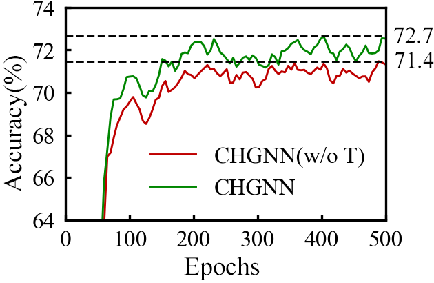
(a) Cora

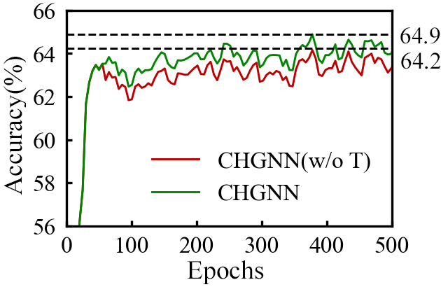
(b) Citeseer

Figure 9: Effect of the enhanced training strategy.

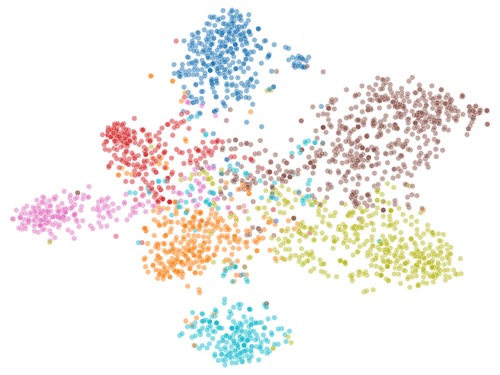
(a) GCN

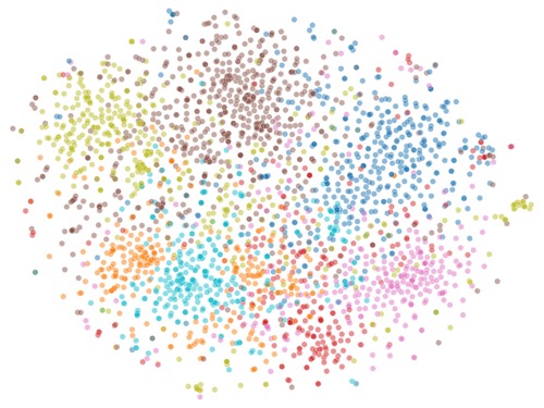
(b) DGI^∗

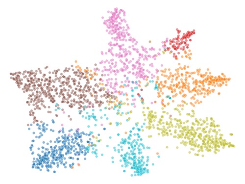
(c) UniGNN

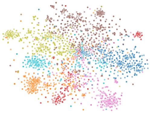
(d) TriCL^∗

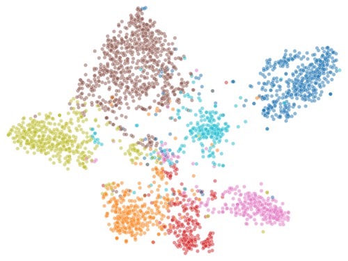
(e) CHGNN

Figure 10: Embedding visualization on CA-Cora (* denotes unsupervised methods).

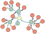
(a) Original

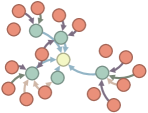
(b) RandAug View1

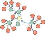
(c) RandAug View2

(d) CHGNN View1

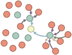
(e) CHGNN View2

Figure 11: Augmenation visualization on CA-Cora.

5.7 Visualization

5.7.1 Embedding Visualization

We visualize the embedding results on CA-Cora by GCN, DGI, UniGNN, TriCL, and CHGNN using the t-SNE method [48] — see Fig. 10. The task-relevance of node embeddings generated by different approaches varies based on the presence of supervision signals. The supervised approaches GCN, UniGNN, and CHGNN generate node embeddings that can be partitioned clearly into seven categories — see Figs. 10 (a), (c), and (e). In contrast, the unsupervised approaches DGI and TriCL tend to exhibit a more uniform distribution of embeddings — see Figs. 10 (b) and (d). The projections of the embeddings generated by CHGNN exhibit more coherent clusters compared with those generated by UniGNN, indicating that CHGNN is better at classifying nodes at class borders. Moreover, joint contrastive losses narrow the distances between embeddings of similar nodes and increase the distances between embeddings of nodes from different classes, which enhances the discriminative power of the embeddings.

5.7.2 Augmentation Visualization

Fig. 11 visualizes the original hypergraph and its augmentation views of a sampling node on CA-Cora. In particular, Fig. 11 (a) is the original sub-hypergraph of the $v$. Figs. 11 (b) and (c) show views generated by RandAug (see Section 5.5), which randomly drops 20% of the hyperedges to obtain two different views [15]. Figs. 11 (d) and (e) show views generated by CHGNN. The yellow circle denotes the sampling node $v$; the green circles denote the hyperedge; and the orange circles denote the 1-hop neighbors of $v$. The label information passed by neighbor nodes is distinguished by colors. The arrows from orange to green circles indicate that the hyperedge contains the neighbor nodes. The arrows from the green to the yellow circle indicate that the hyperedges contain $v$. We see that the views generated by RandAug retain more information on different labels and are almost identical except for two edges. These views preserve substantial non-task dependent and redundant information, which is not beneficial for CL. In contrast, CHGNN View 1 and 2 are less similar to each other, ensuring more variability. In addition, View 1 and 2 both contain key nodes that are essential for node classification.

6 Conclusion

We present CHGNN, a hypergraph neural network model that utilizes CL to learn from labeled and unlabeled data. CHGNN generates hypergraph views using adaptive hypergraph view generators that assign augmentation operations to each hyperedge and performs hypergraph convolution to capture both structural and attribute information of nodes. CHGNN takes advantage of both labeled and unlabeled data during training by incorporating a contrastive loss and a semi-supervised loss. Moreover, CHGNN enhances the training by adaptively adjusting temperature parameters of the contrastive loss functions. This enables learning of node embeddings that better reflect their class memberships. Experiments on nine real-world datasets confirm the effectiveness of CHGNN — it outperforms thirteen state-of-the-art semi-supervised learning and contrastive learning models in terms of classification accuracy. Overall, CHGNN’s performance is particularly robust in scenarios with limited labeled data, making it applicable in many real-world settings. In future research, it is of interest to explore CHGNN on other downstream tasks, e.g., hyperedge prediction, and to extend CHGNN to heterogeneous hypergraphs.

Yumeng Song received the M.S. degree in computer software and theory from Northeastern University, China, in 2019. She is currently working toward her Ph.D. degree in the School of Computer Science and Engineering of Northeastern University. Her current research interests include graph neural networks.

Yu Gu received the Ph.D. degree in computer software and theory from Northeastern University, China, in 2010. He is currently a professor at Northeastern University, China. His current research interests include big data processing, spatial data management, and graph data management. He is a senior member of China Computer Federation (CCF).

Tianyi Li received the Ph.D. degree from Aalborg University, Denmark, in 2022. She is currently an assistant professor with the Department of Computer Science, Aalborg University. Her research concerns spatio-temporal data management and analytics, knowledge integration, and graph neural network. She is a member of IEEE.

Jianzhong Qi received the Ph.D. degree from the University of Melbourne, in 2014. He is a lecturer with the School of Computing and Information Systems, University of Melbourne. He has been an intern with the Toshiba China R&D Center and Microsoft, Redmond, WA, in 2009 and 2013, respectively. His research interests include spatio-temporal databases, location-based social networks, and information extraction.

Zhenghao Liu received the Ph.D. degree in computer software and theory from Tsinghua University, China, in 2021. He is currently an associate professor at Northeastern University, China. His current research interests include artificial intelligence, information retrieval in natural language processing, and automated question and answer.

Christian S. Jensen received the Ph.D. degree from Aalborg University, Denmark, where he is a professor. His research concerns data analytics and management with a focus on temporal and spatiotemporal data. He is a fellow of the ACM and IEEE, and he is a member of the Academia Europaea, the Royal Danish Academy of Sciences and Letters, and the Danish Academy of Technical Sciences.

Ge Yu received the Ph.D. degree in computer science from the Kyushu University of Japan, in 1996. He is currently a professor at the Northeastern University of China. His research interests include distributed and parallel database, data integration, and graph data management. He is a fellow of CCF and a member of the IEEE and ACM.

References

- [1] Y. Feng, H. You, Z. Zhang, R. Ji, and Y. Gao, “Hypergraph neural networks,” in AAAI, 2019, pp. 3558–3565.
- [2] N. Yadati, M. Nimishakavi, P. Yadav, V. Nitin, A. Louis, and P. Talukdar, “HyperGCN: A new method for training graph convolutional networks on hypergraphs,” NeurIPS, vol. 32, 2019.
- [3] J. Han, Q. Tao, Y. Tang, and Y. Xia, “DH-HGCN: Dual homogeneity hypergraph convolutional network for multiple social recommendations,” in SIGIR, 2022, pp. 2190–2194.
- [4] L. Xia, C. Huang, Y. Xu, J. Zhao, D. Yin, and J. Huang, “Hypergraph contrastive collaborative filtering,” in SIGIR, 2022, pp. 70–79.
- [5] J. Yuan, Z. Li, P. Zou, X. Gao, J. Pan, W. Ji, and X. Wang, “Community trend prediction on heterogeneous graph in e-commerce,” in WSDM, 2022, pp. 1319–1327.
- [6] X. Liao, Y. Xu, and H. Ling, “Hypergraph neural networks for hypergraph matching,” in ICCV, 2021, pp. 1266–1275.
- [7] X. Sun, H. Yin, B. Liu, H. Chen, J. Cao, Y. Shao, and N. Q. Viet Hung, “Heterogeneous hypergraph embedding for graph classification,” in WSDM, 2021, pp. 725–733.
- [8] T. N. Kipf and M. Welling, “Semi-supervised classification with graph convolutional networks,” arXiv preprint arXiv:1609.02907, 2016.
- [9] X. Liu, J. Wu, T. Li, L. Chen, and Y. Gao, “Unsupervised entity alignment for temporal knowledge graphs,” arXiv preprint arXiv:2302.00796, 2023.
- [10] Y. Gao, X. Liu, J. Wu, T. Li, P. Wang, and L. Chen, “ClusterEA: Scalable entity alignment with stochastic training and normalized mini-batch similarities,” in KDD, 2022, pp. 421–431.
- [11] J. Huang and J. Yang, “UniGNN: A unified framework for graph and hypergraph neural networks,” in IJCAI, 2021, pp. 2563–2569.
- [12] T. Chen, S. Kornblith, M. Norouzi, and G. Hinton, “A simple framework for contrastive learning of visual representations,” in ICML, 2020, pp. 1597–1607.
- [13] P. Velickovic, W. Fedus, W. L. Hamilton, P. Liò, Y. Bengio, and R. D. Hjelm, “Deep graph infomax.” ICLR (Poster), vol. 2, no. 3, p. 4, 2019.
- [14] Y. You, T. Chen, Y. Sui, T. Chen, Z. Wang, and Y. Shen, “Graph contrastive learning with augmentations,” NeurIPS, vol. 33, pp. 5812–5823, 2020.
- [15] D. Lee and K. Shin, “I’m Me, We’re Us, and I’m Us: Tri-directional contrastive learning on hypergraphs,” in AAAI, 2023.
- [16] X. Xia, H. Yin, J. Yu, Q. Wang, L. Cui, and X. Zhang, “Self-supervised hypergraph convolutional networks for session-based recommendation,” in AAAI, 2021, pp. 4503–4511.
- [17] J. Zhang, M. Gao, J. Yu, L. Guo, J. Li, and H. Yin, “Double-scale self-supervised hypergraph learning for group recommendation,” in CIKM, 2021, pp. 2557–2567.
- [18] Y. Tian, C. Sun, B. Poole, D. Krishnan, C. Schmid, and P. Isola, “What makes for good views for contrastive learning?” NeurIPS, vol. 33, pp. 6827–6839, 2020.
- [19] C. Zhang, S. Hu, Z. G. Tang, and T. H. Chan, “Re-revisiting learning on hypergraphs: Confidence interval and subgradient method,” in ICML, 2017, pp. 4026–4034.
- [20] S. Bai, F. Zhang, and P. H. Torr, “Hypergraph convolution and hypergraph attention,” Pattern Recognition, vol. 110, p. 107637, 2021.
- [21] N. Yadati, “Neural message passing for multi-relational ordered and recursive hypergraphs,” NeurIPS, vol. 33, pp. 3275–3289, 2020.
- [22] E. Chien, C. Pan, J. Peng, and O. Milenkovic, “You are AllSet: A multiset function framework for hypergraph neural networks,” in ICLR, 2022.
- [23] D. Arya, D. K. Gupta, S. Rudinac, and M. Worring, “HyperSAGE: Generalizing inductive representation learning on hypergraphs,” arXiv preprint arXiv:2010.04558, 2020.
- [24] Y. Dong, W. Sawin, and Y. Bengio, “HNHN: Hypergraph networks with hyperedge neurons,” arXiv preprint arXiv:2006.12278, 2020.
- [25] R. Zhang, Y. Zou, and J. Ma, “Hyper-SAGNN: A self-attention based graph neural network for hypergraphs,” arXiv preprint arXiv:1911.02613, 2019.
- [26] Y. Gao, Y. Feng, S. Ji, and R. Ji, “HGNN+: General hypergraph neural networks,” TPAMI, 2022.
- [27] X. Wang, H. Ji, C. Shi, B. Wang, Y. Ye, P. Cui, and P. S. Yu, “Heterogeneous graph attention network,” in The Web Conference, 2019, pp. 2022–2032.
- [28] H. Xue, L. Yang, V. Rajan, W. Jiang, Y. Wei, and Y. Lin, “Multiplex bipartite network embedding using dual hypergraph convolutional networks,” in The Web Conference, 2021, pp. 1649–1660.
- [29] Z. Peng, W. Huang, M. Luo, Q. Zheng, Y. Rong, T. Xu, and J. Huang, “Graph representation learning via graphical mutual information maximization,” in The Web Conference, 2020, pp. 259–270.
- [30] Y. Jiao, Y. Xiong, J. Zhang, Y. Zhang, T. Zhang, and Y. Zhu, “Sub-graph contrast for scalable self-supervised graph representation learning,” in ICDM, 2020, pp. 222–231.
- [31] Y. Zhu, Y. Xu, F. Yu, Q. Liu, S. Wu, and L. Wang, “Graph contrastive learning with adaptive augmentation,” in The Web Conference, 2021, pp. 2069–2080.
- [32] B. Li, B. Jing, and H. Tong, “Graph communal contrastive learning,” in The Web Conference, 2022, pp. 1203–1213.
- [33] K. Hassani and A. H. Khasahmadi, “Contrastive multi-view representation learning on graphs,” in ICML, 2020, pp. 4116–4126.
- [34] Y. Yin, Q. Wang, S. Huang, H. Xiong, and X. Zhang, “AutoGCL: Automated graph contrastive learning via learnable view generators,” in AAAI, 2022, pp. 8892–8900.
- [35] J. Xia, L. Wu, J. Chen, B. Hu, and S. Z. Li, “SimGRACE: A simple framework for graph contrastive learning without data augmentation,” in The Web Conference, 2022, pp. 1070–1079.
- [36] G. Lee, M. Choe, and K. Shin, “How do hyperedges overlap in real-world hypergraphs? -patterns, measures, and generators,” in The Web Conference, 2021, pp. 3396–3407.
- [37] E. Jang, S. Gu, and B. Poole, “Categorical reparameterization with gumbel-softmax,” arXiv preprint arXiv:1611.01144, 2016.
- [38] S. Wan, S. Pan, J. Yang, and C. Gong, “Contrastive and generative graph convolutional networks for graph-based semi-supervised learning,” in AAAI, 2021, pp. 10 049–10 057.
- [39] Y. Li, P. Hu, Z. Liu, D. Peng, J. T. Zhou, and X. Peng, “Contrastive clustering,” in AAAI, 2021, pp. 8547–8555.
- [40] A. v. d. Oord, Y. Li, and O. Vinyals, “Representation learning with contrastive predictive coding,” arXiv preprint arXiv:1807.03748, 2018.
- [41] F. Wang and H. Liu, “Understanding the behaviour of contrastive loss,” in CVPR, 2021, pp. 2495–2504.
- [42] D.-Y. Chen, X.-P. Tian, Y.-T. Shen, and M. Ouhyoung, “On visual similarity based 3D model retrieval,” in Computer graphics forum, vol. 22, no. 3. The Wiley Online Library, 2003, pp. 223–232.
- [43] D. E. Rumelhart, G. E. Hinton, and R. J. Williams, “Learning internal representations by error propagation,” California Univ San Diego La Jolla Inst for Cognitive Science, Tech. Rep., 1985.
- [44] P. Veličković, G. Cucurull, A. Casanova, A. Romero, P. Lio, and Y. Bengio, “Graph attention networks,” arXiv preprint arXiv:1710.10903, 2017.
- [45] M. Zaheer, S. Kottur, S. Ravanbakhsh, B. Poczos, R. R. Salakhutdinov, and A. J. Smola, “Deep sets,” NeurIPS, vol. 30, 2017.
- [46] J. Lee, Y. Lee, J. Kim, A. Kosiorek, S. Choi, and Y. W. Teh, “Set transformer: A framework for attention-based permutation-invariant neural networks,” in ICML, 2019, pp. 3744–3753.
- [47] S.-e. Yoon, H. Song, K. Shin, and Y. Yi, “How much and when do we need higher-order information in hypergraphs? A case study on hyperedge prediction,” in The Web Conference, 2020, pp. 2627–2633.
- [48] L. Van der Maaten and G. Hinton, “Visualizing data using t-SNE.” Journal of machine learning research, vol. 9, no. 11, 2008.