Monte Carlo Grid Dynamic Programming: Almost Sure Convergence and Probability Constraints

Abstract

Dynamic Programming is bedeviled by the ”curse of dimensionality”, which is intensified by the expectations over the process noise. In this paper we present a Monte Carlo-based sampling of the state-space and an interpolation procedure of the resulting value function dependent on the process noise density in a ”self-approximating” fashion. Proof of almost sure convergence is presented. The proposed sampling and interpolation algorithm alleviates the burden of gridding of Dynamic Programming and avoids the construction of a piecewise constant value function over the grid. The sampling nature, and the interpolation procedure of this approach make it adequate to deal with probabilistic constraints.

,

and

1 Introduction

The Dynamic Programming (DP) algorithm [1] is haunted by the curse of dimensionality, which is intensified by the expectations over the process noise [5, ch 25]. Thus, DP is rendered infeasible in many practical problems of interest.

This hedge, into the application of optimal control, had been breached by different methods. For instance, the DP algorithm can be approximated under some stochastic approximation procedures [15], to form what is called Approximate DP [14], or more famously, Reinforcement Learning [10]. Another very successful approach, that is conceptually simple and can handle complex systems and constraints, is model predictive control [7]. Under this approach, a finite-horizon optimal control problem is solved in open-loop, online, i.e. at each time-step, and the first control input in the optimal control sequence is applied. Thus, dodging the need to solve optimal control at many points in the state-space and the need for a function approximation procedure of a value function or an explicit feedback policy over the state-space [9].

Nevertheless, DP is an important algorithm that is still in use in many problems, such as Hamilton-Jacobi Reachability analysis [6]. Moreover, a value function as a measure of goodness and/or safety a state is, in the state-space, can be of a significant importance to a decision maker. Several efficient toolboxes have been developed as optimized DP solvers [4], such toolboxes can work efficiently up to state-dimension 6, as typically reported.

In this paper, we present a Monte-Carlo-based sampling algorithm of the state-space, with an interpolation procedure of the resulting value function and the corresponding feedback law, that is dependent on the process noise density. In [12], a similar randomization and interpolation procedure is presented with its proof of convergence and upper bounds on its computational complexity. Different from [12]: we allow sampling of distributions other than uniform, which is essential, especially when certain regions in the state-space require more attention therefore more samples; importance sampling arguments and the Borel-Cantelli Lemma [11] are used in establishing our proofs; the formulation of the algorithm easily allows the inclusion of probability constraints.

The paper follows a path analogous to that of Bertsekas [2], except, rather than refining the grid to yield a better estimate, we use the Borel-Cantelli lemma to reach similar convergence results, but in the “almost sure” sense. Moreover, the convergence results in this paper are based on estimating a value function represented by a self-approximating interpolation scheme, as described by [12], not a piece-wise constant over the grid as in [2]. We also present a nonlinear $2^{nd}$ order system with probability constraints, showing how the presented algorithms are naturally suitable for dealing with such problems.

2 Finite-Horizon

Consider the finite-horizon optimal control problem of minimizing the cost functional

$$J(x_{0},u_{0:T-1}) =\textbf{E}_{x_{1:T}}\{\sum_{k=1}^{T-1}\ell_{k}(x_{k},u_{k})+\ell_{N}(x_{T})\mid x_{0},u_{0:T-1}\}$$

over the space of finite input sequences $u_{0:T-1}=\{u_{i},\,i\in\mathbb{I}_{T-1}\}$, where $\mathbb{I}_{T}=\{0,1,\ldots,T\}$, subject to: the discrete-time state dynamics

$$x_{k+1}=f(x_{k},u_{k})+w_{k},\,x_{0}\in\mathbb{X}_{0}\subset\mathbb{R}^{r_{x}}\text{is given,}$$ (1)

where $\{w_{k}\}$ is independent and identically distributed according to $\mathcal{W}(.)$; and the input constraints $u_{k}\in U_{k}(x_{k})\subset\mathbb{R}^{r_{u}}$ for all $k\in\mathbb{I}_{N}$, where $U_{k}(x_{k})=\{u_{k}\in\mathbb{U}_{k}\mid\text{Pr}(x_{k+1}\in\mathbb{X}_{k+1}\mid x_{k},u_{k})\geq 1-\epsilon\}$, following a probability constraint [13, 16], is non-empty for all $x_{k}\in\mathbb{X}_{k}\subset\mathbb{R}^{r_{x}}$, $\mathbb{U}_{k}\subset\mathbb{R}^{r_{u}}$ is finite, and $\epsilon\in(0,1)$: the probability of exceeding the state constraints, is predetermined by the user.

The Dynamic Programming algorithm corresponding to this optimal control problem is

$$V_{N}(x_{N}) =\ell_{N}(x_{N}),\,x_{N}\in\mathbb{X}_{N}\subset\mathbb{R}^{r_{x}},$$ (2)

$$V_{k}(x_{k}) =\min_{u_{k}\in U_{k}}\{\ell(x_{k},u_{k})+$$

$$\hskip 56.9055pt\textbf{E}_{x_{k+1}}[V_{k+1}(x_{k+1})\mid x_{k},u_{k}]\},$$ (3)

$$x_{k}\in\mathbb{X}_{k},\,u_{k}\in U_{k}(x_{k}),\,k\in\mathbb{I}_{T},$$ (4)

Assumption 1.

The Euclidean sets $\{\mathbb{X}_{k},\,k\in\mathbb{I}_{T}\}$ are compact.

Assumption 2.

The functions $f(x_{k},u_{k})$ and $\ell(x_{k},u_{k})$ are Lipschitz on $\mathbb{X}_{k}$ for all $k\in\mathbb{I}_{T}$ and $u_{k}\in U_{k}(x_{k})$.

Assumption 3.

$\ell(x_{k},u_{k})\geq 0$ for all $x_{k}\in\mathbb{X}_{k}$ and $u_{k}\in U_{k}(x_{k})$.

Let: $\mathcal{X}_{k}(.)$ be a density function on $\mathbb{X}_{k}$ such that $\textit{supp}(\mathcal{X}_{k})=\mathbb{X}_{k}$, for all $k\in\mathbb{I}_{T}$; the set of particles $\{\xi^{j}_{k}\}_{j=1}^{N_{k}}$ be independent and distributed according to $\mathcal{X}_{k}$, for all $k\in\mathbb{I}_{T}$.

Algorithm 1 Particle Finite-Horizon Dynamic Programming

1:Initialize the set of particles $\{\xi^{j}_{k}\}_{j=1}^{N_{k}}$ in $\mathbb{X}_{k}$, for all $k\in\mathbb{I}_{T}$.

2:Evaluate the weights $\{\Omega^{l}_{T}\}_{l=1}^{N_{T}}$

$$\Omega^{l}_{T}=V_{T}(\xi^{l}_{T})=\ell(\xi^{l}_{T}),\,l=1,\ldots,N_{T}.$$ (5)

3:For each $k=T-1$ down to $k=0$,

$$\Omega^{l}_{k} =\min_{u_{k}\in U_{k}(\xi^{l}_{k})}\{\ell(\xi^{l}_{k},u_{k})+\sum_{j=1}^{N_{k+1}}\Omega^{j}_{k+1}c^{j}(\xi^{l}_{k},u_{k})\},$$ (6)

$$\hskip 14.22636ptl=1,2,\ldots,N_{k},$$

where

$$c^{j}(x_{k},u_{k}) =\frac{\mathcal{W}(\xi^{j}-f(x_{k},u_{k}))}{\sum_{j=1}^{N_{k+1}}\mathcal{W}(\xi^{j}-f(x_{k},u_{k}))}.$$ (7)

We shall show next that Algorithm 1 can be used to generate an approximation $\tilde{V}_{k}^{N_{k}}$,

$$\tilde{V}_{k}^{N_{k}}(x_{k})=\min_{u_{k}\in U_{k}(x_{k})}\{\ell(x_{k},u_{k})+\sum_{j=1}^{N_{k+1}}\Omega^{j}_{k+1}c^{j}(x_{k},u_{k})\},$$ (8)

that converges, almost surely, to $V_{k}(.)$, for all $x_{k}\in\mathbb{X}_{k}$ and $k=1,2,\ldots,T$.

Remark.

The control law corresponding to this approximation of the value function can be found as follows:

$$u_{k}^{*}=\text{arg min}_{u_{k}\in U_{k}(x_{k})}\{\ell(x_{k},u_{k})+\sum_{j=1}^{N_{k+1}}\Omega^{j}_{k+1}c^{j}(x_{k},u_{k})\}$$ (9)

Lemma 1.

The approximation $\tilde{V}_{T-1}^{N_{T-1}}(x_{k})$, in (8), converges, almost surely, to $V_{T-1}(x_{T-1})$ for all $x_{T-1}=\xi_{T-1}^{j},\,j=1,2,\ldots,N_{T-1}$, as $N_{T}\to\infty$.

Proof.

We start with the expectation in the Dynamic Programming Equation (3) for $k=T-1$, i.e.,

$$\textbf{E}_{x_{T}}\{V_{T}(x_{T})\mid x_{T-1},u_{T-1}\}=$$

$$\hskip 14.22636pt\int_{\mathbb{X}_{T}}V_{T}(x_{T})p(x_{T}\mid x_{T-1},u_{T-1})\,dx_{T},$$

where $p(x_{T}\mid x_{T-1},u_{T-1})$ is the prediction density which, for the dynamical system (1), equals $\mathcal{W}(x_{T}-f(x_{T-1},u_{T-1}))$. Since $\{\xi_{T}^{j}\}$ is i.i.d. with density $\mathcal{X}_{T}$ over $\mathbb{X}_{T}$, if the support of the prediction density $\mathcal{W}(\cdot-f(x_{T-1},u_{T-1}))\subset\mathbb{X}_{T}$ for all $x_{T-1}\in\mathbb{X}_{T-1}$ and $u_{T-1}\in U_{T-1}$, then the summation

$$\sum_{j=1}^{N}\Omega^{j}_{T}c^{j}(x_{T-1},u_{T-1}) =\sum_{j=1}^{N}V_{T}(\xi^{j}_{T})c^{j}(x_{T-1},u_{T-1})$$

is the self-normalizing importance sampling estimate [8] of the above expectation. This estimate is unbiased and converges, almost surely, as $N_{T}\to\infty$. Therefore,

$$\ell(\xi^{l}_{T-1},u_{T-1})+\sum_{j=1}^{N_{T}}\Omega^{j}_{T}c^{j}(\xi^{l}_{T-1},u_{T-1})$$

converges, almost surely, to

$$\ell(\xi^{l}_{T-1},u_{T-1})+\textbf{E}_{x_{T}}[V_{T}(x_{T})\mid\xi^{l}_{T-1},u_{T-1}]$$

as $N_{T}\to\infty$, for all $u_{T-1}\in U_{T-1}$ and $\xi^{l}_{T-1},\,l=1,2,\ldots,N_{T-1}$. Since $U_{T-1}(x_{T-1})$ is finite, then the minimum of each of the above over $U_{T-1}(x_{T-1})$ is equal, almost surely, as $N_{T}\to\infty$. ∎

Proposition 1.

The approximation $\tilde{V}_{T-2}^{N_{T-2}}(x_{T-2})$, in (8), converges, almost surely, to $V_{T-2}(x_{T-2})$ for all $x_{T-2}=\xi_{T-2}^{j},\,j=1,2,\ldots,N_{T-2}$, as $N_{T},N_{T-1}\to\infty$.

Proof.

From Lemma 1, we have

$$\lim_{N_{T}\to\infty}\ell(\xi^{l}_{T-2},u_{T-2})+\sum_{j=1}^{N_{T-1}}\Omega^{j}_{T-1}c^{j}(\xi^{l}_{T-2},u_{T-2})$$

$$=\ell(\xi^{l}_{T-2},u_{T-2})+\sum_{j=1}^{N_{T-1}}\lim_{N_{T}\to\infty}\Omega^{j}_{T-1},c^{j}(\xi^{l}_{T-2},u_{T-2})$$

$$=\ell(\xi^{l}_{T-2},u_{T-2})+\sum_{j=1}^{N_{T-1}}V_{T-1}(\xi_{T-1}^{j})c^{j}(\xi^{l}_{T-2},u_{T-2}).$$

Which is the self-normalizing importance sampling estimate [8], since $\text{supp}(\mathcal{W}(\cdot-f(x_{T-2},u_{T-2}))$ for all $x_{T-2}\in\mathbb{X}_{T-1},\,u_{T-2}\in U_{T-2}(x_{T-2})$. Again, this estimate is unbiased and converges, almost surely, to

$$\ell(\xi^{l}_{T-2},u_{T-2})+\textbf{E}_{x_{T-1}}[V_{T-1}(x_{T-1})\mid x_{T-2},u_{T-2}]$$

for all $x_{T-2}\in\mathbb{X}_{T-2}$ and $u_{T-2}\in U_{T-2}(x_{T-2})$. Therefore,

$$\lim_{N_{T},N_{T-1}\to\infty}\min_{u_{T-2}\in U_{T-2}(x_{T-2})}\{\ell(\xi^{l}_{T-2},u_{T-2})+$$

$$\hskip 56.9055pt\sum_{j=1}^{N_{T-1}}\Omega^{j}_{T-1}c^{j}(\xi^{l}_{T-2},u_{T-2})\}$$

$$=\min_{u_{T-2}\in U_{T-2}(x_{T-2})}\{\ell(\xi^{l}_{T-2},u_{T-2})+$$

$$\hskip 56.9055pt\textbf{E}_{x_{T-1}}[V_{T-1}(x_{T-1})\mid\xi^{l}_{T-2},u_{T-2}]\}$$

$$=V_{T-2}(\xi_{T-2}^{l}),\,l=1,2,\ldots,N_{T-2}.$$

∎

Remark.

The necessity of having $\mathcal{W}(\cdot-f(x_{k-1},u_{k-1}))\subset\mathbb{X}_{k}$ for all $k,\,x_{k-1}$ and $u_{k-1}$ might not be possible, for example, due to having Gaussian process noise. This might dictate reformulating the original optimal control problem, for instance, truncating and re-normalizing the densities and/or changing the feasible sets.

Corollary 1.

The approximation $\tilde{V}_{k}^{N_{k}}(x)$, in (8), converges, almost surely, to $V_{k}(x)$ for all $x=\xi_{k}^{j},\,j=1,2,\ldots,N_{k}$, as $N_{T},N_{T-1},\ldots,N_{k}\to\infty$.

Proof.

By induction and using Proposition 1. ∎

Lemma 2.

(Proposition 1 in [2]) $V_{k}(.)$ is Lipschitz on $\mathbb{X}_{k}$ for all $k\in\mathbb{I}_{T}$.

Proof.

Provided in [2], with the therein sum replaced by the expectation in

$$V_{T-1}(x_{T-1}) =\inf_{u_{T-1}\in\mathbb{U}_{T-1}}\textbf{E}_{x_{T}}\{\ell(x_{T-1},u_{T-1})$$

$$\hskip 42.67912pt+V_{T}(x_{T})\mid x_{T-1},u_{T-1}\},$$

$$=\inf_{u_{T-1}\in\mathbb{U}_{T-1}}\{\ell(x_{T-1},u_{T-1})+$$

$$\hskip 42.67912pt\int_{\mathbb{X}_{T}}V_{T}(x_{T})p(x_{T}\mid x_{T-1},u_{T-1})\,dx_{T}\},$$

then all the consequent steps hold true. ∎

Let the sequence of sets $\{A_{j}^{k}\}$, for each $k\in\mathbb{I}_{T}$, be such that

$$A_{k}^{j}=\{x\in\mathbb{X}_{k}:\text{arg}\min_{i\in\mathbb{I}_{N_{k}}}\mid\mid x-\xi_{k}^{j}\mid\mid=j\},$$

where $\mid\mid\cdot\mid\mid$ denotes the Euclidean norm. Then $\{A_{k}^{j},\,j\in\mathbb{I}_{N_{k}}\}$ partitions $\mathbb{X}_{k}$. Also, as in [2], define

$$d_{s}=\max_{k\in\mathbb{I}_{T}}\,\max_{j\in\mathbb{I}_{N}}\,\sup_{x\in A_{j}^{k}}\mid\mid x-\xi_{k}^{j}\mid\mid$$

Lemma 3.

As $N_{k}\to\infty$, $d_{s}\to 0$ almost surely.

Proof.

For any $x\in\mathbb{X}_{k}$, fix $\epsilon>0$. Define the open ball of radius $\epsilon$ and center $x$ as $B_{\epsilon}(x)=\{y\in\mathbb{X}_{k}:\mid\mid y-x\mid\mid<\epsilon\}$. Define the event $C_{j}=[\xi_{j}\in B_{\epsilon}(x)]$. Since $\mathcal{X}_{k}$ is continuous on $\mathbb{X}_{k}$, then $\text{Pr }(C_{j})=\text{constant}>0$. Hence, $\sum_{j=1}^{N_{k}}\text{Pr }(C_{j})\to\infty$ as $N_{k}\to\infty$. By the Borel-Cantelli Zero-One Law [11], $\text{Pr }[C_{j}\text{, infinitely often}]=1$, therefore, there exists some finite positive integer $\bar{N}$, such that $\xi^{\bar{N}}_{k}\in B_{\epsilon}(x)$. This holds for all $\epsilon>0$. ∎

Proposition 2.

The approximation $\tilde{V}_{k}^{N_{k}}(x_{k})$ converges, almost surely, to $V_{k}(x_{k})$, for all $x_{k}\in\mathbb{X}_{k}$, as $N_{k}\to\infty$.

Proof.

For any $x_{k}\in A_{k}^{j}$,

$$\mid\tilde{V}_{k}^{N_{k}}(x_{k})-V_{k}(x_{k})\mid$$

$$\hskip 28.45274pt=\mid\tilde{V}_{k}^{N_{k}}(x_{k})-V_{k}(x_{k})+$$

$$\hskip 56.9055pt\tilde{V}_{k}^{N_{k}}(\xi_{k}^{j})-V_{k}(\xi^{j}_{k})-\tilde{V}_{k}^{N_{k}}(\xi_{k}^{j})+V_{k}(\xi^{j}_{k})\mid,$$

and by applying the triangular inequality, twice,

$$\mid\tilde{V}_{k}^{N_{k}}(x_{k})-V_{k}(x_{k})\mid$$

$$\hskip 28.45274pt\leq\mid\tilde{V}_{k}^{N_{k}}(x_{k})-\tilde{V}_{k}^{N_{k}}(\xi_{k}^{j})\mid+\mid V_{k}(x_{k})-V_{k}(\xi^{j}_{k})\mid$$

$$\hskip 56.9055pt+\mid\tilde{V}_{k}^{N_{k}}(\xi_{k}^{j})-V_{k}(\xi^{j}_{k})\mid.$$

By the Lipschitzness of $\tilde{V}_{k}^{N_{k}}(\cdot)$ and $V_{k}(\cdot)$ on $\mathbb{X}_{k}$,

$$\mid\tilde{V}_{k}^{N_{k}}(x_{k})-\tilde{V}_{k}^{N_{k}}(\xi_{k}^{j})\mid+\mid V_{k}(x_{k})-V_{k}(\xi^{j}_{k})\mid\leq$$

$$\hskip 28.45274pt\mathcal{A}\mid\mid x_{k}-\xi^{j}_{k}\mid\mid+\mathcal{B}\mid\mid x_{k}-\xi^{j}_{k}\mid\mid,$$

for some $\mathcal{A},\,\mathcal{B}>0$, hence

$$\mid\tilde{V}_{k}^{N_{k}}(x_{k})-\tilde{V}_{k}^{N_{k}}(\xi_{k}^{j})\mid+\mid V_{k}(x_{k})-V_{k}(\xi^{j}_{k})\mid\leq$$

$$\hskip 28.45274pt(\mathcal{A}+\mathcal{B})d_{s},$$

which goes to zero, almost surely, as $N_{T},N_{T-1},\ldots,N_{k}\to\infty$. Also, by Corollary 1, $\mid\tilde{V}_{k}^{N_{k}}(\xi_{k}^{j})-V_{k}(\xi^{j}_{k})\mid\to 0$, almost surely, as $N_{T},N_{T-1},\ldots,N_{k}\to\infty$. Therefore, $\mid\tilde{V}_{k}^{N_{k}}(x_{k})-V_{k}(x_{k})\mid$ goes to zero, almost surely, as $N_{T},N_{T-1},\ldots,N_{k}\to\infty$. ∎

3 Infinite-Horizon Discounted Cost

The Dynamic Programming Equation (DPE) of the infinite-horizon discounted cost optimal control problem, for the system described in (1), is [3]

$$V(x_{k}) =\min_{u_{k}\in\mathbb{U}}\{\ell(x_{k},u_{k})+\alpha.\textbf{E}_{x_{k+1}}\{V(x_{k+1})\mid\,x_{k},u_{k}\}\},$$ (10)

$$=\min_{u_{k}\in\mathbb{U}}\{\ell(x_{k},u_{k})+$$

$$\hskip 28.45274pt\alpha.\int_{\mathbb{X}}V(x_{k+1})p(x_{k+1}\mid x_{k},u_{k})\,dx_{k+1}\},$$ (11)

with $\mathbb{X}_{k}=\mathbb{X}$ and $\mathbb{U}_{k}=\mathbb{U}$ for all $k=1,2,\ldots$, and $\mathbb{U}$ is finite. The prediction density $p(x_{k+1}\mid x_{k},u_{k})$

$$p(x_{k+1}\mid x_{k},u_{k})=\mathcal{W}(x_{k+1}-f(x_{k},u_{k})).$$ (12)

The Dynamic Programming algorithm corresponds to the additive cost function is stated as follows:

$$\lim_{T\to\infty}\textbf{E}_{w_{0},\ldots,w_{T}}\left\{\sum_{k=0}^{T}\alpha^{k}\ell(x_{k},u_{k})\right\}.$$ (13)

Suppose that the support of $\mathcal{W}(\cdot-f(x_{k},u_{k}))$ is a subset of $\mathbb{X}$ for all $x_{k}\in\mathbb{X}$ and $u_{k}\in\mathbb{U}$. And suppose that $\{\xi^{j}\in\mathbb{R}^{r_{x}},\,j=1,2,\ldots,N\}$ is independent and distributed according to $\mathcal{X}$, such that the support of $\mathcal{X}$ is $\mathbb{X}$. Then, the following weighted mass density

$$p(x_{k+1}\mid x_{k},u_{k}) =\frac{\sum_{j=1}^{N}\mathcal{W}(\xi^{j}-f(x_{k},u_{k})).\delta(x_{k+1}-\xi^{j}).}{\sum_{m=1}^{N}\mathcal{W}(\xi^{m}-x_{k+1})}$$

$$=\sum_{j=1}^{N}c^{j}(x_{k},u_{k}).\delta(x_{k+1}-\xi^{j})$$ (14)

where

$$c^{j}(x_{k},u_{k}) =\frac{\mathcal{W}(\xi^{j}-f(x_{k},u_{k}))}{\sum_{m=1}^{N}\mathcal{W}(\xi^{m}-f(x_{k},u_{k}))},$$ (15)

is the self-normalized importance sampling approximation of the prediction density in the left-hand-side; since $\text{supp}\mathcal{W}(\cdot-f(x_{k},u_{k})\subset\text{supp}\mathcal{X}(.)$, for all $x_{k},\,u_{k}$.

The following algorithm,

Algorithm 2 Particle Value Iteration

1:Initialize the set of i.i.d. particles $\{\xi^{j}\}_{j=1}^{N}$ according to $\mathcal{X}(\cdot)$ in $\mathbb{X}$,

2:Randomly initialize the weights $\{\Omega^{j}_{0}\}_{j=1}^{N}$ in $\mathbb{R}$, set $i\leftarrow 0$.

3:Update the weights by

$$\Omega^{l}_{i+1} =\min_{u_{k}\in\mathbb{U}}\{\ell(\xi^{l},u_{k})+\alpha.\sum_{j=1}^{N}\Omega^{j}_{i}c^{j}(\xi^{l},u_{k})\},$$ (16)

$$l=1,2,\ldots N$$

4:If $\{\Omega^{j}_{i}\}$ satisfies a convergence criterion as $i$ increases, terminate and set $\Omega^{j}=\Omega^{j}_{i+1}$ for all $j$. Otherwise, set $i\leftarrow i+1$ and go to Step 3.

generates an approximation

$$\tilde{V}^{N}(x)=\min_{u\in\mathbb{U}}\{\ell(x,u)+\alpha.\sum_{j=1}^{N}\Omega^{j}c^{j}(x,u)\}.$$ (17)

Similarly to [2], by the equations (51)-(55) therein, and appealing to Lemma 3 in this paper, it can be shown that

$$\sup_{x\in\mathbb{X}}\mid V(x)-\tilde{V}^{N}(x)\mid\to 0,$$ (18)

almost surely, as $N\to\infty$.

4 Probabilistic Constraints

In this section, we show the two DP algorithms extended to handle probability constraints. This extension is developed for the infinite-horizon algorithm. The application of this extension to the finite-horizon follows naturally.

We start with the optimal control problem introduced in Section 2, but subject to the probabilistic constraints

$$\textbf{Pr}(x_{k}\in\mathbb{S})\geq 1-\epsilon,\text{ for all $k$},$$

where $\mathbb{S}\subset\mathbb{X}$, can be seen as the safe set, which not to be left by the state for more than some probabilistic tolerance $\epsilon\in[0,1)$, supposedly very low. This probability constraint can be augmented to the DP algorithm in Section 2 without a major change; we can restrict the control space to

$$U(x_{k}) =\{u_{k}\in\mathbb{U}_{k}\mid\,\text{Pr}(x_{k+1}\in\mathbb{S}\mid x_{k},u_{k})\geq 1-\epsilon\}.$$ (19)

If $\mathbb{S}$ is a bounded set, the probabilistic constraints can be checked through the Monte Carlo approximations over the state-space grid.

Using the density in (14), the violation probability in (19) is the integral

$$\text{Pr}(x_{k+1}\in\mathbb{S}\mid x_{k},u_{k})=\int_{\mathbb{S}}p(x_{k+1}\mid x_{k},u_{k})\,dx_{k+1}$$ (20)

From the particles $\{\xi^{j}_{k}\}_{j=1}^{N_{k}}$, let the set of indices $\mathbb{I}$ correspond to the particles inside the unsafe set, the complement of $\mathbb{S}$ in $\mathbb{X}$. That is

$$\mathbb{I}=\left\{j\in\{1,\ldots,N\}\mid\xi^{j}\in\mathbb{S}^{c}\right\}.$$

The violation probability is then approximated by

$$\text{Pr}(x_{k+1}\in\mathbb{S}^{c}\mid x_{k},u_{k})=\sum_{j\in\mathbb{I}}c^{j}(x_{k},u_{k}),$$ (21)

hence, the input constraint set (19) is then replaced by

$$U^{N}(x_{k}) =\{u_{k}\in\mathbb{U}_{k}\mid\,\sum_{j\in\mathbb{I}}c^{j}(x_{k},u_{k})<\epsilon\}.$$ (22)

Algorithm 3 Particle Value Iteration with probabilistic constraints

1:Initialize the set of i.i.d. particles $\{\xi^{j}\}_{j=1}^{N}$ according to $\mathcal{X}(\cdot)$ in $\mathbb{X}$,

2:Identify the set $\mathbb{I}$,

3:Randomly initialize the weights $\{\Omega^{j}_{0}\}_{j=1}^{N}$ in $\mathbb{R}$, set $i\leftarrow 0$.

4:Update the weights by

$$\Omega^{l}_{i+1} =\min_{u_{k}\in U^{N}(\xi^{l})}\{\ell(\xi^{l},u_{k})+\alpha.\sum_{j=1}^{N}\Omega^{j}_{i}c^{j}(\xi^{l},u_{k})\},$$ (23)

$$l=1,2,\ldots N$$

5:If $\{\Omega^{j}_{i}\}$ satisfies a convergence criterion as $i$ increases, terminate and set $\Omega^{j}=\Omega^{j}_{i+1}$ for all $j$. Otherwise, set $i\leftarrow i+1$ and go to Step 3.

5 Numerical Examples

Two numerical examples are presented in this section. The first example is a simple scalar linear Gaussian state-space model in which infinite-horizon discounted cost value function is known and can be compared to that generated by Algorithm 2. The second example is a two states nonlinear system which is to respect some probability constraint.

5.1 Discounted cost LQR

Consider the following linear Gaussian state-space model:

$$x_{k+1}=Fx_{k}+Gu_{k}+w_{k},\,w_{k}\sim\mathcal{N}(\mu_{w},W),$$ (24)

with full state feedback, i.e., $y_{k}=x_{k}$.

The infinite horizon, discounted-cost LQR [3] value function can be found by solving the following DPE:

$$V(x_{k}) =\min_{u}\{x_{k}^{T}Qx_{k}+u_{k}^{T}Ru_{k}+$$

$$\hskip 28.45274pt\alpha.\textbf{E}_{w_{k}}\{V(Fx_{k}+Bu_{k}+w_{k})\}\},$$

where the value function has the form $V(x_{k})=x_{k}^{T}Xx_{k}+q$ for some positive definite matrix $X$ and constant $q>0$.

The matrix $X$ can be found by solving the following Algebraic Riccati Equation:

$$X=\alpha F^{T}XF-\alpha^{2}A^{T}XB(R+\alpha B^{T}XB)^{-1}B^{T}XA+Q,$$ (25)

and

$$q=\frac{\alpha}{1-\alpha}\text{trace}\{XW\}.$$ (26)

Now for (24), suppose

$$x_{k+1}=0.95x_{k}+u_{k}+w_{k},\,w_{k}\sim\mathcal{N}(0,0.5\,\mathbb{I}_{3\times 3}).$$ (27)

and $Q=R=1$. The value function, after substituting the corresponding values in (25) and (26), is

$$V(x_{k})=1.460x_{k}^{2}+6.570.$$

Towards comparing the above value function to a one acquired by Algorithm 2: we use $2000$ particles $\{\xi^{j}\}_{j=1}^{2000}$ where $\xi^{j}\sim\mathcal{N}(0,4)$, and sampled control actions $\{\nu^{j}\}_{j=1}^{50}$ such that $\nu^{j}\sim\mathcal{N}(0,1)$. Value Iteration via Algorithm 2 is then conducted, and the resulting particle value function is approximated by the quadratic polynomial

$$V(x_{k})=1.410x_{k}^{2}-0.0023x_{k}+5.52.$$

The feedback control law of the particle approximation as in (9) is compared to the discounted-cost LQR controller. This is shown in Figure 1.

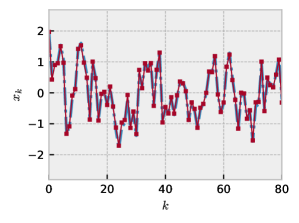
Figure 1: The response of the linear Gaussian system (27), with identical initial conditions disturbance realizations, to each: the exact LQR optimal control (in blue), and the particle approximation (9) (in red).

5.2 Nonlinear system with probabilistic constraints

Given the dynamics:

$$x^{1}_{k+1} =0.9x^{1}_{k}+0.2x^{2}_{k}+w_{k}^{1},$$

$$x^{2}_{k+1} =-0.15x^{1}_{k}+0.9x^{2}_{k}+0.05x^{1}_{k}x^{2}_{k}+u_{k}+w_{k}^{2},$$

where $x_{k}=(x^{1}_{k},x^{2}_{k})^{T}$ is the state vector, and the disturbance, $(w_{k}^{1},w_{k}^{2})^{T}=w_{k}\sim\mathcal{N}(0,.3\mathbb{I}_{2\times 2})$, is white. To better visualize the dynamics, Figure 2 represents the streamlines of the state dynamics with zero input and state disturbances.

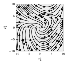
Figure 2: The streamlines of the difference vector field $f(x_{k},u_{k},w_{k})-x_{k}$ with $u_{k}$ and $w_{k}$ set to zero.

Suppose the L-shaped state set, $\mathcal{L}=[3,5]\times[-4,2]\cup[-2,5]\times[-7,-4]$, is to be avoided, that is, $\mathbb{S}$ is the complement of $\mathcal{L}$ in $\mathbb{X}$.

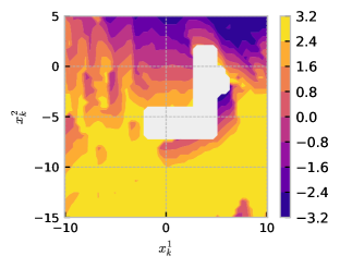
Figure 3: Colormap of $\kappa$ acquired by Algorithm 3 and fitted by a piece-wise surface. White regions correspond to infeasible states.

Towards defining an optimal control law $\kappa$, let $V$ be the value function, the optimal cost, of the infinite horizon discounted cost whose stage costs are $\ell_{k}(x_{k},u_{k})=x_{k}^{T}x_{k}+u_{k}^{2}$ and with a discount factor $\gamma=0.9$ [3]. Following the Value Iteration in Algorithm 3, uniformly randomized grids of $2000$ points over $\mathbb{X}=[-10,10]\times[-5,15]$ and $50$ points in $\mathbb{U}=[-3,3]$, are generated. Convergence is considered achieved if the maximum absolute relative error is less than $5\%$. Figure 3 shows the colormap of the resulting $\kappa$, and the empty regions are infeasible states. A Pythoncode of this example can be found at https://github.com/msramada/MC_DynamicProgramming.

6 Conclusion

The convergence of the value function and feedback law approximants to their continuous state and input spaces counterparts is implied under regularity conditions. This number is highly dependent on the corresponding dimension of these spaces and the complexity of the involved dynamics and distributions. Hence, the curse of dimensionality cannot be avoided by this approach. However, the flexibility of the sampling procedure and the self-approximating forms provided alleviate some burden in the implementation of DP and make it more natural to handle constraints of probabilistic nature. Regions of the state-space of higher importance can tantamount to regions of higher distribution in the sampling procedure.

References

- [1] Richard E Bellman and Stuart E Dreyfus. Applied dynamic programming. Princeton university press, 2015.
- [2] Dimitri Bertsekas. Convergence of discretization procedures in dynamic programming. IEEE Transactions on Automatic Control, 20(3):415–419, 1975.
- [3] Dimitri Bertsekas. Dynamic programming and optimal control: Volume I, volume 1. Athena scientific, 2012.
- [4] M. Chen. “Optimized Dynamic Programming-Based Algorithms Solver”.
- [5] Arnaud Doucet, Nando De Freitas, Neil James Gordon, et al. Sequential Monte Carlo methods in practice, volume 1. Springer, 2001.
- [6] Sylvia Herbert, Jason J Choi, Suvansh Sanjeev, Marsalis Gibson, Koushil Sreenath, and Claire J Tomlin. Scalable learning of safety guarantees for autonomous systems using hamilton-jacobi reachability. arXiv preprint arXiv:2101.05916, 2021.
- [7] SSa Keerthi and Elmer G Gilbert. Optimal infinite-horizon feedback laws for a general class of constrained discrete-time systems: Stability and moving-horizon approximations. Journal of optimization theory and applications, 57(2):265–293, 1988.
- [8] Jun S Liu and Jun S Liu. Monte Carlo strategies in scientific computing, volume 10. Springer, 2001.
- [9] David Q Mayne. Model predictive control: Recent developments and future promise. Automatica, 50(12):2967–2986, 2014.
- [10] Benjamin Recht. A tour of reinforcement learning: The view from continuous control. Annual Review of Control, Robotics, and Autonomous Systems, 2:253–279, 2019.
- [11] Sidney Resnick. A probability path. Springer, 2019.
- [12] John Rust. Using randomization to break the curse of dimensionality. Econometrica: Journal of the Econometric Society, pages 487–516, 1997.
- [13] Alexander T Schwarm and Michael Nikolaou. Chance-constrained model predictive control. AIChE Journal, 45(8):1743–1752, 1999.
- [14] Jennie Si, Andrew G Barto, Warren B Powell, and Don Wunsch. Handbook of learning and approximate dynamic programming, volume 2. John Wiley & Sons, 2004.
- [15] Christopher JCH Watkins and Peter Dayan. Q-learning. Machine learning, 8(3-4):279–292, 1992.
- [16] Jun Yan and Robert R Bitmead. Incorporating state estimation into model predictive control and its application to network traffic control. Automatica, 41(4):595–604, 2005.