Solving Strongly Convex and Smooth Stackelberg Games Without Modeling the Follower

Abstract

Stackelberg games have been widely used to model interactive decision-making problems in a variety of domains such as energy systems, transportation, cybersecurity, and human-robot interaction. However, existing algorithms for solving Stackelberg games often require knowledge of the follower’s cost function or learning dynamics and may also require the follower to provide an exact best response, which can be difficult to obtain in practice. To circumvent this difficulty, we develop an algorithm that does not require knowledge of the follower’s cost function or an exact best response, making it more applicable to real-world scenarios. Specifically, our algorithm only requires the follower to provide an approximately optimal action in response to the leader’s action. The inexact best response is used in computing an approximate gradient of the leader’s objective function, with which zeroth-order bilevel optimization can be applied to obtain an optimal action for the leader. Our algorithm is proved to converge at a linear rate to a neighborhood of the optimal point when the leader’s cost function under the follower’s best response is strongly convex and smooth.

I Introduction

Stackelberg games have recently been used as a mathematical formulation for a number of tasks in energy systems [19, 16, 18, 1], transportation [20, 23], cybersecurity [14], and human-robot interaction [13, 11, 17]. In a two-player Stackelberg game, one player, which is commonly referred to as the leader, is trying to minimize her cost assuming the other player, which is commonly referred to as the follower, is taking his optimal action after observing the leader’s action. In other words, the follower chooses a best response to the leader’s action. The Stackelberg game can also be viewed as a special case of bilevel optimization [3].

Many learning algorithms for Stackelberg games or, more generally, bilevel optimization, require knowing the follower’s cost function. For example, Fiez et al. [7] developed a learning algorithm for two-player Stackelberg games that locally converges to an optimal solution. In their algorithm, both the follower and the leader use the gradient descent algorithm, in which the leader uses an inexact gradient that depends on the first-order and second-order information on the follower’s cost function. Chen et al. [2] made the same assumption that the follower’s cost function is known and speeded up the algorithm by Fiez et al. by adding a predictive term to the follower’s learning dynamics.

When the follower’s cost function is unknown, existing algorithms require knowledge of the follower’s learning dynamics. For example, Conn et al. [4] designed a learning algorithm for bilevel optimization that does not require first-order information on the follower’s cost function. However, they also designed the follower’s learning dynamics so that the follower is capable of providing an inexact best response. The inexact best response from the designed learning dynamics can be used by the leader to update her action. There are many ways to design the follower’s dynamics that yield an inexact best response; see [10, 22]. There are also algorithms for bilevel optimization that do not rely on designing the follower’s dynamics. However, those algorithms assume specific forms of either the follower’s optimization problem (e.g., a linear program [21]) or the leader’s problem (e.g., a least-squares problem [6]).

Assumptions of a known cost function or known learning dynamics are often made to the follower in previous works on Stackelberg games. However, these assumptions do not hold in many cases. For instance, in human-robot interaction, the follower is a human agent, whose cost function may not be known, and whose learning dynamics may not follow what is given by existing learning algorithms. Furthermore, humans do not always provide a best response, such a phenomenon is known as bounded rationality. Therefore, it is important to consider and relax these assumptions to effectively design autonomous systems that can collaborate with human agents. Existing work on Stackelberg games with a human follower typically assumes that the follower’s cost function is given or attempts to learn the cost function by, e.g., inverse reinforcement learning [8, 15]. Some results do not assume knowing the follower’s cost function but assume that the follower always provides an exact best response [12, 11].

Contribution

In this paper, we make an initial attempt to relax the current assumptions on the follower when solving two-player Stackelberg games. In particular, our problem setup makes the following assumptions:

1. The follower’s cost function is unknown and does not follow a specific form.

2. The follower’s learning dynamics are unknown and cannot be designed by us.

3. The follower only gives an inexact best response that is $\varepsilon$ close to the exact best response (to be defined formally in Section III-A).

Our end result is a gradient-based learning algorithm that is guaranteed to converge to a neighborhood of the optimal point at a linear rate, where the size of the neighborhood depends on the inexactness $\varepsilon$ of the best response oracle. Our algorithm is tested numerically for quadratic cost functions, and the numerical simulation results are consistent with our theoretical analysis.

II Background: Stackelberg Games

We consider a two-player Stackelberg game, where $x\in\mathbb{R}^{n}$ is the leader’s action, and $y\in\mathbb{R}^{m}$ is the follower’s action. The goal of the leader is to minimize her cost $f_{1}$ assuming that the follower will take the best response, i.e., the follower’s action is optimal with respect to the follower’s cost function given a leader’s action. Mathematically, the leader attempts to solve the following bilevel optimization problem:

$$\underset{x\in\mathbb{R}^{n}}{\min.}\quad f(x)\triangleq f_{1}(x,r(x)),$$ (1)

where $r(x)=\operatorname*{arg\,min}_{y\in\mathbb{R}^{m}}f_{2}(x,y)$ is the best response of the follower. In this paper, we assume that the minimizer of $f_{2}(x,\cdot)$ is unique for each $x$ to ensure that the best response function $r$ is well-defined. We denote $D_{j}f_{i}(\cdot,\cdot)$ as the derivative mapping of $f_{i}$ on the $j$-th argument, where $i=1,2$ and $j=1,2$. The derivative mapping of the best response $r$ is denoted as $Dr$. The optimal solution of (1) is denoted as $x^{\star}$.

The Stackelberg game formulation (1) can be used for modeling a variety of tasks. For example, in human-robot collaboration, the robot is modeled as the leader and the human as the follower. With a human follower, we typically have access to the exact zeroth-order and first-order information of the leader’s cost function $f_{1}$, but the follower’s cost function $f_{2}$ and best response function $r$ are typically unknown. We adopt these settings on $f_{1}$, $f_{2}$, and $r$ together with the following assumptions:

Assumption 1.

$D_{1}f_{1}(x,\cdot)$ is $L_{f_{1}}^{x}$-Lipschitz, and $D_{2}f_{1}(x,\cdot)$ is $L_{f_{1}}^{y}$-Lipschitz for any $x$.

Assumption 2.

The best response function $r$ is differentiable, and $\|Dr(x)\|\leq R_{1}$ for any $x$.

Assumption 3.

The best response function $r$ is $R_{2}$-smooth, i.e., $Dr$ is $R_{2}$-Lipschitz continuous.

Throughout this paper, we use $\|\cdot\|$ to denote the $L_{2}$-norm for vectors and the induced $L_{2}$-norm for matrices.

Assumption 1 is a common assumption in bilevel optimization and Stackelberg games; see [3] and [7]. Assumptions 2 and 3 imply that the follower does not change his action rapidly when the leader’s action changes.

III Proposed Framework

In this section, we give a gradient-based algorithm in Section III-A that uses an inexact gradient derived in Section III-B to solve (1). Computing the inexact gradient requires that the follower give an inexact best response to the leader’s action, as defined in Section III-A.

III-A Inexact Best Response

Our algorithm relies on the simple fact that the inexact best response should be close to the exact best response. A formal definition is given as follows.

Definition 1.

A follower’s action $y$ is called an $\varepsilon$-inexact best response ($\varepsilon$-IBR) to a leader’s action $x$ if $\|y-r(x)\|\leq\varepsilon$.

If the follower uses gradient descent to compute an $\varepsilon$-IBR when the leader’s action $x$ is fixed, i.e., $y_{t+1}=y_{t}-\beta D_{2}f_{2}(x,y_{t})$, where $\beta$ is a stepsize, then condition $\|y_{t}-r(x)\|<\varepsilon$ can be verified by the quantity $\|y_{t}-y_{t-1}\|$ if $f_{2}(x,\cdot)$ is strongly convex for any $y$.

We choose to avoid defining the inexact best response as a function $y\colon\mathbb{R}^{n}\rightarrow\mathbb{R}^{m}$ such that for some constant $\varepsilon>0$, the function $y$ satisfies $\|y(x)-r(x)\|\leq\varepsilon$ for any $x$. For tasks in HRI, this would imply that the human’s actions follow a function of the robot’s actions. In other words, each robot’s action would correspond to a specific and deterministic action of the human, thus imposing a strong assumption on the human’s behavior.

Our gradient-based algorithm is given by

$$x^{k+1}=x^{k}-\alpha g_{x^{k}},$$ (2)

where $k=1,2,\dots$ is the index of iteration. The stepsize $\alpha$ is a fixed constant that should be chosen small enough; the specific choice of $\alpha$ will be discussed in Section IV-C. The term $g_{x^{k}}$ is an inexact gradient at $x^{k}$. From the decomposition of the exact gradient mapping

$$\nabla f(x)=D_{1}f_{1}(x,r(x))+D_{2}f_{1}(x,r(x))Dr(x),$$ (3)

an estimation $g_{x}$ is given by

$$g_{x}=D_{1}f_{1}(x,y)+D\hat{\psi}_{x},$$ (4)

where $D_{1}f_{1}(x,y)$ approximates $D_{1}f_{1}(x,r(x))$, and $D\hat{\psi}_{x}$ approximates $D_{2}f_{1}(x,r(x))Dr(x)$. The follower’s action $y$ is an $\varepsilon$-IBR of the leader’s action $x$. The computation of $D\hat{\psi}_{x}$ only requires an inexact best response of the follower. Detail will be given in Section III-B.

III-B Computing an Inexact Gradient

Throughout this subsection, we denote the point where we perform gradient estimation as $x_{0}$, i.e., we would like to use $g_{x_{0}}$ as an estimate of $\nabla f(x_{0})$. First, define

$$Df_{1}(x,y)\triangleq D_{1}f_{1}(x,y)+D_{2}f_{1}(x,y)Dr(x).$$

Thus, we can approximate $\nabla f(x_{0})$ based on the above formula to obtain

$$\nabla f(x_{0})=Df_{1}(x_{0},r(x_{0}))\approx Df_{1}(x_{0},y_{0})$$ (5)

$$\qquad=D_{1}f_{1}(x_{0},y_{0})+D_{2}f_{1}(x_{0},y_{0})Dr(x_{0}).$$ (6)

The part $D_{1}f_{1}(x_{0},r(x_{0}))$ can be approximated by $D_{1}f_{1}(x_{0},y_{0})$, where $y_{0}$ is an $\varepsilon$-IBR of $x_{0}$. Similarly, to approximate the second part, define $\psi(x)\triangleq D_{2}f_{1}(x_{0},y_{0})r(x).$ Note that the definition of $\psi(x)$ depends on $(x_{0},y_{0})$. Since $D_{2}f_{1}(x_{0},y_{0})Dr(x_{0})=\nabla\psi(x_{0}),$ we can approximate $D_{2}f_{1}(x_{0},r(x_{0}))Dr(x_{0})$ by a finite-difference approximation of $\psi$, which requires evaluating $\psi$ at points near $x_{0}$. However, an exact evaluation of $\psi$ is not possible, since we do not have the exact best response $r$. To circumvent this issue, we approximate $\psi(x)$ by $\hat{\psi}_{x}\triangleq D_{2}f_{1}(x_{0},y_{0})y$, where $y$ is an $\varepsilon$-IBR of $x$. Define each $x_{i}$ as

$$x_{i}=x_{0}+\delta v_{i},\quad i=1,2,\ldots,p,$$ (7)

where $v_{i}$’s is a positive basis of $\mathbb{R}^{n}$. (See [5, Section 2.1] for the definition of a positive basis.) Our goal is to approximate $D_{2}f_{1}(x_{0},r(x_{0}))Dr(x_{0})$ from $\{(x_{0},y_{0}),(x_{1},y_{1}),\ldots,(x_{p},y_{p})\}$, where each $y_{i}$ is an $\varepsilon$-IBR of $x_{i}$. Our approximator $D\hat{\psi}_{x_{0}}$ for $D_{2}f_{1}(x_{0},r(x_{0}))Dr(x_{0})$ is given by

$$D\hat{\psi}_{x_{0}} =\operatorname*{arg\,min}_{D\hat{\psi}}\left\|\left[\begin{array}[]{c}\hat{\psi}_{x_{0}}\\ \hat{\Psi}_{x_{0}}\end{array}\right]-\left[\begin{array}[]{cc}\mathbf{1}_{p+1}&M\end{array}\right]\left[\begin{array}[]{c}\hat{\psi}_{x_{0}}\\ D\hat{\psi}\end{array}\right]\right\|$$ (13)

$$=\operatorname*{arg\,min}_{D\hat{\psi}}\|\hat{\Psi}_{x_{0}}-MD\hat{\psi}\|,$$ (14)

where $\hat{\Psi}_{x_{0}}=(\hat{\psi}_{x_{1}},\ldots,\hat{\psi}_{x_{p}})^{\top},$ and

$$\quad M=\left[\begin{array}[]{c}0\\ \delta V\end{array}\right],\qquad V=[v_{1},\ldots,v_{p}]^{\top}.$$

IV Main Results

In this section, we show that (2) converges at a linear rate. The difference between (2) and the standard gradient descent is that the gradient (4) used in (2) is inexact. Thus, if the inexact gradient (4) is close to the true gradient, a convergence result similar to the standard gradient descent is expected. In Section IV-A, we adopt the proof in [5, Theorem 2.13] to show that the difference between the inexact gradient computed by (4) and the true gradient is upper bounded. The upper bound relies on a function that can be further upper bounded by a function of $\|\nabla f(x)\|$ based on Assumption 4. The meaning of Assumption 4 will be discussed in detail in Section IV-B. By using the upper bound constructed in Section IV-A, we establish a similarity between (2) and the standard gradient descent and give a proof of convergence for (2) in Section IV-C.

IV-A Upper Bounding the Error of the Inexact Gradient

The following proposition shows that the error of the inexact gradient is upper bounded.

Proposition 1.

Suppose $f_{1}$ and $f_{2}$ satisfy Assumptions 1, 2, and 3. The inexact gradient $g_{x}$ defined in (4) satisfies

$$\|\nabla f(x)-g_{x}\|\leq\varphi(x)$$ (15)

for all $x$, where

$$\varphi(x)\triangleq a\varepsilon+b\|D_{2}f_{1}(x,r(x))\|$$ (16)

with $a=L_{f_{1}}^{y}R_{1}+L_{f_{1}}^{x}+bL_{f_{1}}^{y}$  and $b=\sqrt{p+1}(\delta^{2}R_{2}+\varepsilon)\|M^{\dagger}\|/2$.

Proof.

By definition, at any point $x_{0}$

$$\|\nabla f(x_{0})-g_{x_{0}}\|$$ (17)

$$\qquad\leq\|D_{1}f_{1}(x_{0},r(x_{0}))-D_{1}f_{1}(x_{0},y_{0})\|$$

$$\qquad\quad+\|D_{2}f_{1}(x_{0},r(x_{0}))Dr(x_{0})-D\hat{\psi}_{x_{0}}\|.$$

The first part of the right-hand side of (17) can be bounded as

$$\|D_{1}f_{1}(x_{0},r(x_{0}))-D_{1}f_{1}(x_{0},y_{0})\| \leq L_{f_{1}}^{x}\|r(x_{0})-y_{0}\|$$ (18)

$$\leq L_{f_{1}}^{x}\varepsilon.$$ (19)

Define $\Psi_{x_{0}}=(\psi(x_{1}),\ldots,\psi(x_{p}))^{\top}$, where each $x_{i}$ is defined in (7). The second part of the right-hand side of  (17) is bounded by

$$\|D_{2}f_{1}(x_{0},r(x_{0}))Dr(x_{0})-D\hat{\psi}_{x_{0}}\|\\ \qquad\leq\|D_{2}f_{1}(x_{0},r(x_{0}))Dr(x_{0})-D_{2}f_{1}(x_{0},y_{0})Dr(x_{0})\|\\ \qquad\quad+\|D_{2}f_{1}(x_{0},y_{0})Dr(x_{0})-D\hat{\psi}_{x_{0}}\|.$$ (20)

The first part of (20) can be bounded by

$$\|D_{2}f_{1}(x_{0},r(x_{0}))Dr(x_{0})-D_{2}f_{1}(x_{0},y_{0})Dr(x_{0})\|$$ (21)

$$\qquad\leq\|D_{2}f_{1}(x_{0},r(x_{0}))-D_{2}f_{1}(x_{0},y_{0})\|\|Dr(x_{0})\|$$ (22)

$$\qquad\leq L_{f_{1}}^{y}R_{1}\varepsilon.$$ (23)

The second part of (20) can be bounded by

$$\|D_{2}f_{1}(x_{0},y_{0})Dr(x_{0})-D\hat{\psi}_{x_{0}}\|$$ (24)

$$\qquad=\|\nabla\psi(x_{0})-D\hat{\psi}_{x_{0}}\|$$ (25)

$$\qquad\leq\left\|\left[\begin{array}[]{c}\psi(x_{0})\\ \nabla\psi(x_{0})\end{array}\right]-D\hat{\psi}_{x_{0}}\right\|$$ (28)

$$\qquad=\left\|\left[\begin{array}[]{c}\psi(x_{0})\\ \nabla\psi(x_{0})\end{array}\right]-M^{\dagger}\hat{\Psi}_{x_{0}}\right\|$$ (31)

$$\qquad\leq\left\|\left[\begin{array}[]{c}\psi(x_{0})\\ \nabla\psi(x_{0})\end{array}\right]-M^{\dagger}\Psi_{x_{0}}\right\|+\|M^{\dagger}\Psi_{x_{0}}-M^{\dagger}\hat{\Psi}_{x_{0}}\|.$$ (34)

To bound $\left\|\left[\begin{array}[]{c}\psi(x_{0})\\ \nabla\psi(x_{0})\end{array}\right]-M^{\dagger}\Psi_{x_{0}}\right\|$, define

$$h\triangleq M\left[\begin{array}[]{c}\psi(x_{0})\\ \nabla\psi(x_{0})\end{array}\right]-\Psi_{x_{0}}.$$ (35)

Thus,

$$|h_{i}| =|\psi(x_{0})-\psi(x_{i})+\langle\nabla\psi(x_{0}),x_{i}-x_{0}\rangle|$$ (36)

$$=\left|\int_{0}^{1}\langle\nabla\psi(x_{0})\right.$$ (37)

$$\qquad-\left.\nabla\psi(x_{0}+t(x_{i}-x_{0})),x_{i}-x_{0}\rangle\,dt\right|$$ (38)

$$\leq\|x_{i}-x_{0}\|\int_{0}^{1}\|\nabla\psi(x_{0})-\nabla\psi(x_{0}+t(x_{i}-x_{0}))\|\,dt$$ (39)

$$\leq\|x_{i}-x_{0}\|\|D_{2}f_{1}(x_{0},y_{0})\|$$ (40)

$$\qquad\cdot\int_{0}^{1}\|Dr(x_{0})-Dr(x_{0}+t(x_{i}-x_{0}))\|\,dt$$ (41)

$$\leq\|x_{i}-x_{0}\|^{2}\|D_{2}f_{1}(x_{0},y_{0})\|R_{2}\int_{0}^{1}t\,dt$$ (42)

$$=\frac{\delta^{2}R_{2}\|D_{2}f_{1}(x_{0},y_{0})\|}{2}.$$ (43)

From (35),

$$\left\|\left[\begin{array}[]{c}\psi(x_{0})\\ \nabla\psi(x_{0})\end{array}\right]-M^{\dagger}\Psi_{x_{0}}\right\| =\|M^{\dagger}h\|.$$ (46)

Also,

$$\|M^{\dagger}h\| \leq\|M^{\dagger}\|\|h\|$$ (47)

$$\leq\sqrt{\dim(h)}\frac{\delta^{2}R_{2}}{2}\|M^{\dagger}\|\|D_{2}f_{1}(x_{0},y_{0})\|$$ (48)

$$=\frac{\sqrt{p+1}}{2}\delta^{2}R_{2}\|M^{\dagger}\|(\|D_{2}f_{1}(x_{0},r(x_{0}))\|+L_{f_{1}}^{y}\varepsilon).$$ (49)

Finally, we can bound $\|M^{\dagger}\Psi_{x_{0}}-M^{\dagger}\hat{\Psi}_{x_{0}}\|$ by

$$\|M^{\dagger}\Psi_{x_{0}}-M^{\dagger}\hat{\Psi}_{x_{0}}\|$$ (50)

$$\qquad\leq\|M^{\dagger}\|\|\Psi_{x_{0}}-\hat{\Psi}_{x_{0}}\|$$ (51)

$$\qquad\leq\frac{\sqrt{p+1}}{2}\|M^{\dagger}\|\|D_{2}f_{1}(x_{0},y_{0})\|\varepsilon$$ (52)

$$\qquad\leq\frac{\sqrt{p+1}}{2}\varepsilon\|M^{\dagger}\|(\|D_{2}f_{1}(x_{0},r(x_{0}))\|+L_{f_{1}}^{y}\varepsilon).$$ (53)

Combine (19), (23), (49), and (53) to obtain

$$\|\nabla f(x_{0})-g_{x_{0}}\|$$ (54)

$$\qquad\leq L_{f_{1}}^{x}\varepsilon+L_{f_{1}}^{y}R_{1}\varepsilon$$ (55)

$$\qquad\quad+\frac{\sqrt{p+1}}{2}\delta^{2}R_{2}\|M^{\dagger}\|(\|D_{2}f_{1}(x_{0},r(x_{0}))\|+L_{f_{1}}^{y}\varepsilon)$$ (56)

$$\qquad\quad+\frac{\sqrt{p+1}}{2}\varepsilon\|M^{\dagger}\|(\|D_{2}f_{1}(x_{0},r(x_{0}))\|+L_{f_{1}}^{y}\varepsilon)$$ (57)

$$\qquad=L_{f_{1}}^{x}\varepsilon+L_{f_{1}}^{y}R_{1}\varepsilon$$ (58)

$$\qquad\quad+\frac{\sqrt{p+1}}{2}\|M^{\dagger}\|(\delta^{2}R(\|D_{2}f_{1}(x_{0},r(x_{0}))\|+L_{f_{1}}^{y}\varepsilon)$$ (59)

$$\qquad\quad+\varepsilon(\|D_{2}f_{1}(x_{0},r(x_{0}))\|+L_{f_{1}}^{y}\varepsilon))$$ (60)

$$\qquad=L_{f_{1}}^{x}\varepsilon+L_{f_{1}}^{y}R_{1}\varepsilon+\frac{\sqrt{p+1}}{2}(\delta^{2}R_{2}+\varepsilon)\|M^{\dagger}\|$$ (61)

$$\qquad\qquad\cdot(\varepsilon L_{f_{1}}^{y}+\|D_{2}f_{1}(x_{0},r(x_{0}))\|).$$ (62)

Since $x_{0}$ is arbitrary, the proof is finished. ∎

The value of $\|M^{\dagger}\|$ in the upper bound given in Proposition 1 can be calculated once a positive basis is chosen. The following corollary gives an expression of $\|M^{\dagger}\|$ under the positive basis that consists of the standard basis and the negative standard basis.

Corollary 1.

Choose each $v_{i}$ as the positive basis defined as

$$V=[\begin{array}[]{cccc}v_{1}&v_{2}&\ldots&v_{2n}\end{array}]^{\top}=\left[\begin{array}[]{cc}I_{n}&-I_{n}\end{array}\right].$$ (63)

In this case,

$$M=\left[\begin{array}[]{c}0\\ \delta I_{n}\\ -\delta I_{n}\end{array}\right].$$ (64)

We have $\varphi(x)=a\varepsilon+b\|D_{2}f_{1}(x,r(x))\|$ with $a=L_{f_{1}}^{y}R_{1}+L_{f_{1}}^{x}+bL_{f_{1}}^{y}$  and $b=\sqrt{4n+2}\left(\varepsilon/\delta+\delta R_{2}\right)/4$.

Proof.

Denote by $\sigma_{\max}(\cdot)$ and $\sigma_{\min}(\cdot)$ the maximum and minimum singular values of a matrix, respectively. Notice $M^{T}M=2\delta^{2}I$. This implies $\sigma_{\min}(M)=\sqrt{2}\delta$. Use the fact $\sigma_{\max}(M^{\dagger})=1/\sigma_{\min}(M)$ to obtain $\|M^{\dagger}\|=\sqrt{2}/(2\delta)$. ∎

IV-B Bounded Sensitivity

The only non-constant term in the upper bound given in (16) is $\|D_{2}f_{1}(x_{0},r(x_{0}))\|$. To upper bound this term, we make the following assumption.

Assumption 4 (Bounded sensitivity).

There exists a constant $\kappa>0$ such that $\|D_{2}f_{1}(x,r(x))\|\leq\kappa\|\nabla f(x)\|$ for any $x$.

With Assumption 4, this term can be further bounded by $\kappa\|\nabla f(x_{0})\|$, after which techniques for analyzing the standard gradient descent algorithm can be applied (see Section IV-C). This subsection will discuss the practical implications of Assumption 4.

Recall that the exact gradient of (1) is defined as

$$\nabla f(x)=D_{1}f_{1}(x,r(x))+D_{2}f_{1}(x,r(x))Dr(x).$$ (65)

Under Assumption 4 and Assumption 2,

$$\|D_{2} f_{1}(x,r(x))\|$$ (66)

$$\leq\kappa\|D_{1}f_{1}(x,r(x))+D_{2}f_{1}(x,r(x))Dr(x)\|$$ (67)

$$\leq\kappa(\|D_{1}f_{1}(x,r(x))\|+\|D_{2}f_{1}(x,r(x))\|R_{1}).$$ (68)

Rearrange the above equation to obtain

$$\frac{1}{\kappa}\leq\frac{\left\|D_{1}f_{1}(x,r(x))\right\|}{\left\|D_{2}f_{1}(x,r(x))\right\|}+R_{1}$$ (69)

when $\kappa\neq 0$ and $\|D_{2}f_{1}(x,r(x))\|\neq 0$. The ratio $\left\|D_{1}f_{1}(x,r(x))\right\|/\left\|D_{2}f_{1}(x,r(x))\right\|$ characterizes the sensitivity of the leader’s cost to the follower’s action relative to the leader’s action when the follower chooses the best response. Based on (69), a smaller $\kappa$ implies that the leader’s cost is less sensitive to the follower’s action. The existence of $\kappa$ implies that the sensitivity is bounded, hence the name bounded sensitivity assumption for Assumption 4.

Another intuitive way to understand the bounded sensitivity assumption is to consider fully collaborative Stackelberg games, where $f_{1}=f_{2}$. In this setting, when the follower takes the best response, the leader’s cost is only affected by her own action, which implies $\kappa=0$. Formally, since $r(x)$ is the follower’s best response to $x$, the optimality condition of the follower’s optimization problem is given by $D_{2}f_{2}(x,r(x))=0$. When $f_{1}=f_{2}$, the optimality condition implies $D_{2}f_{1}(x,r(x))=0$, allowing one to choose $\kappa=0$ to satisfy Assumption 4.

IV-C Convergence Analysis for Strongly Convex and Smooth Cost

Under Assumption 4 and Proposition 1, we can prove formally that our algorithm converges linearly to a neighborhood of $x^{\star}$ by using a similar technique for analyzing standard gradient descent with strongly convex and smooth functions [9].

Theorem 1.

Suppose the follower gives an $\varepsilon$-IBR in every step, and the leader uses stepsize $\alpha<1/L_{f}$. Also, assume that $f$ is $\mu_{f}$-strongly convex and $L_{f}$-smooth, and $f_{1}$ and $f_{2}$ satisfy Assumptions 1, 2, 3, and 4. Let $a=L_{f_{1}}^{y}R_{1}+L_{f_{1}}^{x}+bL_{f_{1}}^{y}$, and $b=\sqrt{p+1}(\delta^{2}R_{2}+\varepsilon)\|M^{\dagger}\|/2$. The algorithm given by (2) and (4) converges to a neighborhood of $f^{\star}$ with the following property:

$$\limsup_{k\rightarrow\infty}(f(x_{k+1})-f^{\star})\leq\frac{(2ab\kappa\varepsilon+a^{2}\varepsilon^{2})}{2\mu_{f}(1-b^{2}\kappa^{2}-2ab\kappa\varepsilon)}$$

if

$$b^{2}\kappa^{2}+2ab\kappa\varepsilon-1<0.$$ (70)

Proof.

By the Lipschitz continuity of $\nabla f$, we have

$$f(x_{k+1})-f(x_{k})$$ (71)

$$\qquad\leq\langle\nabla f(x_{k}),x_{k+1}-x_{k}\rangle+\frac{L_{f}}{2}\|x_{k+1}-x_{k}\|^{2}$$ (72)

$$\qquad=-\alpha\langle\nabla f(x_{k}),g(x_{k})\rangle+\frac{\alpha^{2}L_{f}}{2}\|g(x_{k})\|^{2}$$ (73)

By (15),

$$\varphi(x_{k})^{2} \geq\|\nabla f(x_{k})-g(x_{k})\|^{2}$$ (74)

$$=\|\nabla f(x_{k})\|^{2}+\|g(x_{k})\|^{2}-2\langle\nabla f(x_{k}),g(x_{k})\rangle.$$ (75)

Rearrange the above inequality to obtain

$$-2\langle\nabla f(x_{k}),g(x_{k})\rangle\\ \qquad\leq\varphi(x_{k})^{2}\ -\|\nabla f(x_{k})\|^{2}-\|g(x_{k})\|^{2}.$$ (76)

Substituting (76) into (71) gives

$$f(x_{k+1})-f(x_{k})\\ \leq-\frac{\alpha}{2}\|\nabla f(x_{k})\|^{2}+\left(\frac{\alpha^{2}L_{f}}{2}-\frac{\alpha}{2}\right)\|g(x_{k})\|^{2}\\ +\frac{\alpha\varphi(x_{k})^{2}}{2}.$$ (77)

From (77),

$$f(x_{k+1})-f(x_{k})$$ (78)

$$\qquad\leq-\frac{\alpha}{2}\|\nabla f(x_{k})\|^{2}+\frac{\alpha\varphi(x_{k})^{2}}{2}$$ (79)

$$\qquad\leq-\frac{\alpha}{2}\|\nabla f(x_{k})\|^{2}+\frac{\alpha}{2}(a\varepsilon+b\kappa\|\nabla f(x_{k})\|)^{2}$$ (80)

$$\qquad=-\frac{\alpha}{2}((1-b^{2}\kappa^{2})\|\nabla f(x_{k})\|^{2}-a^{2}\varepsilon^{2}$$ (81)

$$\qquad\quad-2ab\kappa\varepsilon\|\nabla f(x_{k})\|).$$ (82)

Since $b^{2}\kappa^{2}+2ab\kappa\varepsilon-1<0$, if $\|\nabla f(x_{k})\|\geq 1$

$$f(x_{k+1})-f(x_{k})$$ (83)

$$\qquad\leq-\frac{\alpha}{2}((1-b^{2}\kappa^{2})\|\nabla f(x_{k})\|^{2}$$ (84)

$$\qquad\quad-2ab\kappa\varepsilon\|\nabla f(x_{k})\|^{2})+\frac{\alpha a^{2}\varepsilon^{2}}{2}$$ (85)

$$\qquad\leq\mu_{f}\alpha(b^{2}\kappa^{2}+2ab\kappa\varepsilon-1)(f(x_{k})-f^{\star})$$ (86)

$$\qquad\quad+\frac{\alpha a^{2}\varepsilon^{2}}{2},$$ (87)

else if $\|\nabla f(x)\|\leq 1$, we have

$$f(x_{k+1})-f(x_{k})$$ (88)

$$\qquad\leq-\frac{\alpha}{2}(\|\nabla f(x_{k})\|^{2}-b^{2}k^{2}\|\nabla f(x_{k})\|^{2})$$ (89)

$$\qquad\quad+\frac{\alpha}{2}(2ab\kappa\varepsilon+a^{2}\varepsilon^{2})$$ (90)

$$\qquad\leq\mu_{f}\alpha(b^{2}k^{2}-1)(f(x_{k})-f^{\star})$$ (91)

$$\qquad\quad+\frac{\alpha}{2}(2ab\kappa\varepsilon+a^{2}\varepsilon^{2}).$$ (92)

Rearrange and subtract $f^{\star}$ on each side of the above formula to obtain

$$f(x_{k+1})-f^{\star}\leq(1+\mu_{f}\alpha(b^{2}\kappa^{2}+2ab\kappa\varepsilon-1))\\ \qquad\quad\cdot(f(x_{k})-f^{\star})+\frac{\alpha}{2}(2ab\kappa\varepsilon+a^{2}\varepsilon^{2}).$$ (93)

Note that $\alpha\leq 1/L_{f}\leq 1/\mu_{f}$. Thus,  $1>1+\mu_{f}\alpha(b^{2}\kappa^{2}+2ab\kappa\varepsilon-1)\geq 0$. Take $f(x_{k})-f^{\star}$ as a Lyapunov function $V(x_{k})$ finishes the proof. ∎

The theorem shows that the algorithm in (2) converges to a neighborhood of $x^{\star}$ linearly. Because $b^{2}\kappa^{2}+2ab\kappa\varepsilon-1$ is an increasing function of $\varepsilon$, condition (70) can always be satisfied if $\varepsilon$ is small enough. We will discuss more on the effect of $\varepsilon$ in Section V.

V Numerical Simulation

In this section, we test our algorithm when both players use a convex quadratic cost. Formally, we define $f_{i}\colon\mathbb{R}^{n}\times\mathbb{R}^{m}\rightarrow\mathbb{R}$ for $i=1,2$ such that

$$f_{i}(x,y)=\frac{1}{2}\left[\begin{array}[]{l}x\\ y\end{array}\right]^{\top}\left[\begin{array}[]{cc}P_{i}&Q_{i}\\ Q_{i}^{\top}&R_{i}\end{array}\right]\left[\begin{array}[]{l}x\\ y\end{array}\right],$$ (94)

where

$$\left[\begin{array}[]{cc}P_{i}&Q_{i}\\ Q_{i}^{\top}&R_{i}\end{array}\right]$$ (95)

is positive definite. We adopt the same positive basis defined in Corollary 1 to compute the inexact gradient $g_{x}$ defined by (4). Note that

$$\nabla f(x)=\left(P_{1}-Q_{1}R_{2}^{-1}Q_{2}^{\top}+Q_{2}R_{2}^{-1}R_{1}^{\top}R_{2}^{-1}Q_{2}^{\top}\right)x$$

and $D_{2}f_{1}(x,r(x))=\left(P_{1}-Q_{1}R_{2}^{-1}Q_{2}^{\top}\right)x.$ Thus, $\kappa$ can be computed by

$$\kappa =\frac{\sigma_{\max}\left(P_{1}-Q_{1}R_{2}^{-1}Q_{2}^{\top}+Q_{2}R_{2}^{-1}R_{1}^{\top}R_{2}^{-1}Q_{2}^{\top}\right)}{\sigma_{\min}\left(P_{1}-Q_{1}R_{2}^{-1}Q_{2}^{\top}\right)},$$ (96)

where $\sigma_{\max}(\cdot)$ and $\sigma_{\min}(\cdot)$ are the maximum and minimum singular values of the corresponding matrix. Also, we restrict our simulation to the case that $P_{1}-Q_{1}R_{2}^{-1}Q_{2}^{\top}+Q_{2}R_{2}^{-1}R_{1}^{\top}R_{2}^{-1}Q_{2}^{\top}$ is positive definite to match the strong convexity assumption made in Section IV-C.

V-A The Effect of Inexact Best Response

We chose the sampling radius $\delta$ as $\delta=0.1$, the stepsize $\alpha$ as $\alpha=0.01$, and the total number of iterations as $1000$. For the problem instance and the parameters we chose, condition (70) is satisfied for $\varepsilon<0.447$. Fig. 1 shows $\|x-x^{\star}\|$, the distance between our iterate and the optimal point, versus the number of iterations under different choices of $\varepsilon$. As the plot shows, the algorithm converges to a neighborhood of $x^{\star}$ at a linear rate. Also, for a larger $\varepsilon$, the steady-state error becomes larger.

For $\varepsilon=0.01$, $0.025$, and $0.04$, the result that the steady-state error increases with $\varepsilon$ is consistent with the upper bound

$$\frac{\left(2ab\kappa\varepsilon+a^{2}\varepsilon^{2}\right)}{2\mu_{f}\left(1-b^{2}\kappa^{2}-2ab\kappa\varepsilon\right)}$$ (97)

given in Theorem 1, which is an increasing function of $\varepsilon$ when condition (70) is satisfied. However, the numerical experiment suggests that condition (70) given in Theorem 1 may not be necessary for convergence, as shown in Fig. 1 when $\varepsilon=0.1$ and $0.2$.

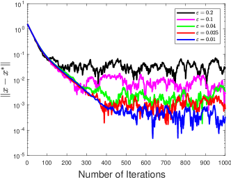
Figure 1: Effect of $\varepsilon$ on the convergence of (2). The steady-state error increases as $\varepsilon$ increases.

V-B Tightness of Error Bound

In this subsection, we will investigate the tightness of the theoretical error bound (97) given in Theorem 1 when condition (70) is satisfied. We calculated the gap between the theoretical error bound and the actual error, i.e.,

$$\frac{\left(2ab\kappa\varepsilon+a^{2}\varepsilon^{2}\right)}{2\mu_{f}\left(1-b^{2}\kappa^{2}-2ab\kappa\varepsilon\right)}-(f(x_{T})-f^{\star})$$ (98)

under different choices of $\varepsilon$, where $T$ represents the total number of iterations.

It is easy to verify that (97) tends to $0$ as $\varepsilon$ tends to $0$, which implies that the error bound is tight for $\varepsilon=0$, i.e., when the follower gives the exact best response. However, our numerical experiment suggests that the theoretical upper bound is loose when $\varepsilon>0$, as shown by the relationship between the gap (98) and $\varepsilon$ given in Fig. 2. In addition, the gap (98) increases as $\varepsilon$ increases, which suggests that the theoretical upper bound (97) in Theorem 1 becomes more conservative as $\varepsilon$ increases.

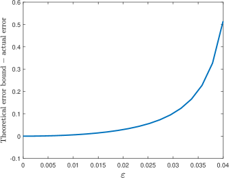
Figure 2: Effect of $\varepsilon$ on the tightness of the theoretical error bound when $\delta=0.1$. The theoretical error bound becomes more conservative as $\varepsilon$ increases.

VI Conclusions

This paper presents an algorithm for solving Stackelberg games that relaxes several common assumptions in the literature on the follower. Unlike previous work that requires knowledge of the cost function or learning dynamics of the follower, our algorithm only requires the follower to provide an approximate best response under any action played by the leader. This is particularly relevant to interactive decision-making problems in which the follower deviates from rationality and/or has an unknown cost function, for example, when the follower is a human agent. We have shown both theoretically and numerically that our algorithm converges to a neighborhood of the optimal solution at a linear rate.

References

- [1] Ralf Borndörfer, Bertrand Omont, Guillaume Sagnol, and Elmar Swarat. A Stackelberg Game to Optimize the Distribution of Controls in Transportation Networks. In Vikram Krishnamurthy, Qing Zhao, Minyi Huang, and Yonggang Wen, editors, Game Theory for Networks, Lecture Notes of the Institute for Computer Sciences, Social Informatics and Telecommunications Engineering, pages 224–235, Berlin, Heidelberg, 2012. Springer.
- [2] Tianyi Chen, Yuejiao Sun, Quan Xiao, and Wotao Yin. A Single-Timescale Method for Stochastic Bilevel Optimization. In Proceedings of The 25th International Conference on Artificial Intelligence and Statistics, pages 2466–2488. PMLR, May 2022.
- [3] Benoît Colson, Patrice Marcotte, and Gilles Savard. An overview of bilevel optimization. Annals of Operations Research, 153(1):235–256, September 2007.
- [4] A. R. Conn and L. N. Vicente. Bilevel derivative-free optimization and its application to robust optimization. Optimization Methods and Software, 27(3):561–577, June 2012.
- [5] Andrew R. Conn, Katya Scheinberg, and Luis N. Vicente. Introduction to Derivative-Free Optimization. Society for Industrial and Applied Mathematics, January 2009.
- [6] Matthias J. Ehrhardt and Lindon Roberts. Inexact Derivative-Free Optimization for Bilevel Learning. Journal of Mathematical Imaging and Vision, 63(5):580–600, June 2021.
- [7] Tanner Fiez, Benjamin Chasnov, and Lillian Ratliff. Implicit Learning Dynamics in Stackelberg Games: Equilibria Characterization, Convergence Analysis, and Empirical Study. In Proceedings of the 37th International Conference on Machine Learning, pages 3133–3144. PMLR, November 2020.
- [8] Dylan Hadfield-Menell, Stuart J. Russell, Pieter Abbeel, and Anca Dragan. Cooperative inverse reinforcement learning. Advances in neural information processing systems, 29, 2016.
- [9] Hamed Karimi, Julie Nutini, and Mark Schmidt. Linear Convergence of Gradient and Proximal-Gradient Methods Under the Polyak-Łojasiewicz Condition. In Paolo Frasconi, Niels Landwehr, Giuseppe Manco, and Jilles Vreeken, editors, Machine Learning and Knowledge Discovery in Databases, volume 9851, pages 795–811. Springer International Publishing, Cham, 2016.
- [10] Ayalew Getachew Mersha and Stephan Dempe. Direct search algorithm for bilevel programming problems. Computational Optimization and Applications, 49(1):1–15, May 2011.
- [11] Stefanos Nikolaidis, Jodi Forlizzi, David Hsu, Julie Shah, and Siddhartha Srinivasa. Mathematical Models of Adaptation in Human-Robot Collaboration, August 2017.
- [12] Stefanos Nikolaidis, David Hsu, and Siddhartha Srinivasa. Human-robot mutual adaptation in collaborative tasks: Models and experiments. The International Journal of Robotics Research, 36(5-7):618–634, June 2017.
- [13] Stefanos Nikolaidis, Swaprava Nath, Ariel D. Procaccia, and Siddhartha Srinivasa. Game-Theoretic Modeling of Human Adaptation in Human-Robot Collaboration. In Proceedings of the 2017 ACM/IEEE International Conference on Human-Robot Interaction, pages 323–331, March 2017.
- [14] Jeffrey Pawlick, Edward Colbert, and Quanyan Zhu. A Game-theoretic Taxonomy and Survey of Defensive Deception for Cybersecurity and Privacy. ACM Comput. Surv., 52(4):82:1–82:28, August 2019.
- [15] Dorsa Sadigh, Shankar Sastry, Sanjit A. Seshia, and Anca D. Dragan. Planning for autonomous cars that leverage effects on human actions. In Robotics: Science and Systems, volume 2, pages 1–9. Ann Arbor, MI, USA, 2016.
- [16] Hichem Sedjelmaci, Makhlouf Hadji, and Nirwan Ansari. Cyber Security Game for Intelligent Transportation Systems. IEEE Network, 33(4):216–222, July 2019.
- [17] Ran Tian, Liting Sun, Andrea Bajcsy, Masayoshi Tomizuka, and Anca D. Dragan. Safety Assurances for Human-Robot Interaction via Confidence-aware Game-theoretic Human Models. In 2022 International Conference on Robotics and Automation (ICRA), pages 11229–11235, May 2022.
- [18] Kun Wang, Li Yuan, Toshiaki Miyazaki, Yuanfang Chen, and Yan Zhang. Jamming and Eavesdropping Defense in Green Cyber–Physical Transportation Systems Using a Stackelberg Game. IEEE Transactions on Industrial Informatics, 14(9):4232–4242, September 2018.
- [19] Yunpeng Wang, Walid Saad, Zhu Han, H. Vincent Poor, and Tamer Başar. A Game-Theoretic Approach to Energy Trading in the Smart Grid. IEEE Transactions on Smart Grid, 5(3):1439–1450, May 2014.
- [20] Hai Yang, Xiaoning Zhang, and Qiang Meng. Stackelberg games and multiple equilibrium behaviors on networks. Transportation Research Part B: Methodological, 41(8):841–861, October 2007.
- [21] M. Hosein Zare, Oleg A. Prokopyev, and Denis Sauré. On Bilevel Optimization with Inexact Follower. Decision Analysis, 17(1):74–95, March 2020.
- [22] Dali Zhang and Gui-Hua Lin. Bilevel direct search method for Leader–Follower problems and application in health insurance. Computers & Operations Research, 41:359–373, January 2014.
- [23] Xiaoning Zhang, H.M. Zhang, Hai-Jun Huang, Lijun Sun, and Tie-Qiao Tang. Competitive, cooperative and Stackelberg congestion pricing for multiple regions in transportation networks. Transportmetrica, 7(4):297–320, July 2011.