Efficient simulation of individual-based population models: the R Package IBMPopSim

Daphné Giorgi Laboratoire de Probabilités, Statistique et Modélisation, Sorbonne Université and Université Paris Cité, CNRS, F-75005 Paris, France. Sarah Kaakai Laboratoire Manceau de Mathématiques & FR CNRS 2962, Institut du Risque et de l’Assurance, Le Mans Université, Le Mans, France. Vincent Lemaire Laboratoire de Probabilités, Statistique et Modélisation, Sorbonne Université and Université Paris Cité, CNRS, F-75005 Paris, France.
Abstract

The R Package IBMPopSim111see also https://daphnegiorgi.github.io/IBMPopSim/ aims to simulate the random evolution of heterogeneous populations using stochastic Individual-Based Models (IBMs). The package enables users to simulate population evolution, in which individuals are characterized by their age and some characteristics, and the population is modified by different types of events, including births/arrivals, death/exit events, or changes of characteristics. The frequency at which an event can occur to an individual can depend on their age and characteristics, but also on the characteristics of other individuals (interactions). Such models have a wide range of applications. For instance, IBMs can be used for simulating the evolution of a heterogeneous insurance portfolio with selection or for validating mortality forecasts.

IBMPopSim overcomes the limitations of time-consuming IBMs simulations by implementing new efficient algorithms based on thinning methods, which are compiled using the Rcpp package while providing a user-friendly interface.

Keywords: Individual-based models, stochastic simulation, population dynamics, Poisson measures, thinning method, actuarial science, insurance portfolio simulation.

1 Introduction

In various fields, advances in probability have contributed to the development of a new mathematical framework for so-called individual-based stochastic population dynamics, also called stochastic Individual-Based Models (IBMs). These models are initially developed in a Markovian setup in view of applications in mathematical biology and ecology. After the pioneer works [FM04, Tra06, CFM06] there is a large community that has used this formalism for the study of the evolution of structured populations (see e.g. [FT09, CMM13, CHLM16, BCF+16, LSA+19, MRR19, CIH+20, RJMR22]. Many mathematical results have been obtained to describe qualitatively the limit behaviors of such stochastic systems: in long time or in large population for example. We refer to the reference book [BM15] for more details on these mathematical results. But the simulation of large and interacting populations is expensive and the package IBMPopSim can meet many needs in this community.

In a quite different field, IBMs have been used to study human populations and to calculate demographic indicators for actuarial purposes or to take into account longevity risk in financial products. We refer to [Ben10, Bou16, EHK21] for some applications in this field. Stochastic IBMs allow the modeling in continuous time of populations dynamics structured by age and/or characteristics (gender, socioeconomic status, frailty…). There are other domains in which this modeling based on individuals is used, for example in epidemiology with the stochastic SIR model  or in social sciences in particular for demographic applications.

To be more precise the mathematical model of an IBM is a measure-valued Markov process with jumps. We use a pathwise representation driven by Poisson point measures to obtain efficient simulation algorithms. This pathwise representation based on the thinning method for Poisson random measures allows to rewrite an IBM as a continuous-time Markov chain in a general space.

For demographic applications that do not involve interactions in the population, the R package MicSim [Zin14] implements microsimulation, which may seem similar to IBM simulation. Here we point out a major difference between the two approaches. In continuous-time microsimulation, individual life-courses are usually specified by sequences of state transitions (events) and the time spans between these transitions. The state space is usually discrete and finite. Microsimulation involves producing all individual lifelines, which is possible when there are no interactions. Once all the individual life events are generated, we can observe the population’s evolution over time (by adding births or entries in the population). In contrast, in an IBM approach, the population is constantly evolving, and the next time of change in the population is obtained as a time of competition between the different events that can occur in the population.

We chose to use the Rcpp package to implement the algorithms of the IBMPopSim package. Rcpp is a package for the R programming language that enables integration of C++ code into R. It provides a powerful interface for seamless integration of C++ code with R, allowing R users to write high-performance code in C++ that can be easily called from R. Our package provides easy-to-use R functions for defining the events that occur in the population and their intensities. Users have the flexibility to define their own events using just a few lines of C++ code. Once these events and intensities are defined, a model is created that consists of C++ source code, which is compiled using Rcpp and integrated into the R session. This code can then be called with different parameters to quickly produce population evolution scenarios. Numerous examples are provided in the form of R vignettes on the website https://daphnegiorgi.github.io/IBMPopSim/.

In Section 2, we provide a brief overview of Poisson random measures and introduce the thinning method in a general context. In Section 3, we present the mathematical framework for the IBM and present the algorithms used in this package. In Section 4, we present the main functions of the IBMPopSim package, which allow for the definition of events and their intensities, the creation of a model, and the simulation of scenarios. In Section 5, we provide a first example of applying the package to simulate an insurance portfolio with entry and exit events. Finally, in Section 6, we conclude with the simulation of an interacting age-structured population with genetically variable traits.

2 Preliminaries on Random counting measures

We begin by reviewing some useful properties of Poisson random measures, mainly following Chapter 6 of [Çin11]. Other useful reference on this important field of random measures is [Kal17]. In the following, we denote by $(\Omega,\{\mathcal{F}_{t}\},{\mathbb{P}})$ the filtered probability space and $(E,\mathcal{E})$ a Borel subspace of $({\mathbb{R}}^{d},\mathcal{B}({\mathbb{R}}^{d}))$.

A random counting measure allows the representation of a random set $S=\{X_{k},\;k\geq 1\}\subset E$ as an integer-valued measure $Q:\Omega\times E\to\bar{\mathbb{N}}$ where for $A\in\mathcal{E}$, $Q(A)$ is the (random) number of random variables $X_{k}$ in the subset $A$. Formally, the random counting measure $Q$, also called simple point process, is defined by

$$Q(A)=\sum_{k\geq 1}\boldsymbol{1}_{A}(X_{k})\quad\forall A\in\mathcal{E},\text{ i.e. }Q=\sum_{k\geq 1}\delta_{X_{k}}.$$ (1)

Random integrals of positive measurable functions are then defined by

$$Q(f)=\int_{E}f(x)Q(\mathrm{d}x)=\sum_{k\geq 1}f(X_{k}).$$

Note that if $Q$ is a random counting measure and $\Delta$ is a measurable random set, then the restriction $Q^{\Delta}=\boldsymbol{1}_{\Delta}Q$ of $Q$ to $\Delta$ (counting only atoms $X_{i}$ in the set $\Delta$) is obviously also a random counting measure.

2.1 Poisson Random measures

An important example of random counting measures are Poisson random measures.

Definition 2.1 (Poisson Random measures).

Let $\mu$ be a $\sigma$-finite diffuse measure on $(E,\mathcal{E})$. A random counting measure $Q$ is a Poisson (counting) random measure of mean measure $\mu$ if

  1. 1.

    $\forall A\in\mathcal{E}$, $Q(A)$ is a Poisson random variable with ${\mathbb{E}}[Q(A)]=\mu(A)$.

  2. 2.

    For all disjoints subsets $A_{1},\dots,A_{n}\in\mathcal{E}$, $Q(A_{1}),\dots,Q(A_{n})$ are independent Poisson random variables.

Let us briefly recall here some simple but useful operations on Poisson measures.

Proposition 2.2 (Restricted Poisson measure).

If $B\in\mathcal{E}$, then, the restriction of $Q$ to $B$ defined by

$$Q^{B}=\boldsymbol{1}_{B}Q=\sum_{k\geq 1}\mathbf{1}_{B}(X_{k})\delta_{X_{k}}$$

is also a Poisson random measure, of mean measure $\mu^{B}=\mu(\cdot\cap B)$.

Proposition 2.3 (Projection of Poisson measure).

If $E=F_{1}\times F_{2}$ is a product space, then the projection

$$Q_{1}(\mathrm{d}x)=\int_{F_{2}}Q(\mathrm{d}x,\mathrm{d}y)$$ (2)

is a Poisson random measure of mean measure $\mu_{1}(\mathrm{d}x)=\int_{F_{2}}\mu(\mathrm{d}x,\mathrm{d}y)$.

Link with Poisson processes

Let $Q=\sum_{k\geq 1}\delta_{T_{k}}$ a Poisson random measure on $E={\mathbb{R}}^{+}$ with mean measure $\mu(\mathrm{d}t)=\Lambda(t)\mathrm{d}t$ absolutely continuous with respect to the Lebesgue measure ($\mu(A)=\int_{A}\Lambda(t)\mathrm{d}t$). The counting process $(N_{t})_{t\geq 0}$ defined by

$$N_{t}=Q([0,t])=\sum_{k\geq 1}\boldsymbol{1}_{\{T_{k}\leq t\}},\quad\forall\;t\geq 0,$$ (3)

is an inhomogeneous Poisson process with intensity function (or rate) $t\mapsto\Lambda(t)$.

In particular, when $\Lambda(t)\equiv c$ is a constant, $N$ is a homogeneous Poisson process with rate $c$. Assuming that the atoms are ordered $T_{1}<T_{2}<\dots$, we recall that the sequence $(T_{k+1}-T_{k})_{k\geq 1}$ is a sequence of i.i.d. exponential variables of parameter $c$.

Poisson Random measures on $E={\mathbb{R}}^{+}\times F$

We are interested in the particular case when $E$ is the product space ${\mathbb{R}}^{+}\times F$, with $(F,\mathcal{F})$ a Borel subspace of ${\mathbb{R}}^{d}$. Then, a random measure $Q$ is defined from a random set $S=\{(T_{k},Y_{k}),k\geq 1\}$. The random variables $T_{k}\geq 0$ can be considered as time variables, and constitute the jump times of the random measure, while the $Y_{k}\in F$ represent space variables.

We recall in this special case the Theorem VI.3.2 (called main Theorem) in [Çin11].

Proposition 2.4.

Let $m$ be a $\sigma$–finite diffuse measure on ${\mathbb{R}}^{+}$, and $K$ a transition probability kernel from $({\mathbb{R}}^{+},\mathcal{B}({\mathbb{R}}^{+}))$ into $(F,\mathcal{F})$. Assume that the collection $(T_{k})_{k\geq 1}$ forms a Poisson random measure with mean $m$, and given $(T_{k})_{k\geq 1}$, the variables $Y_{k}$ are conditionally independent and have the respective distributions $K(T_{k},\cdot)$.

  1. 1.

    Then, $(T_{k},Y_{k})_{k\geq 1}$ forms a Poisson random measure $Q=\sum_{k\geq 1}\delta_{(T_{k},Y_{k})}$ on $({\mathbb{R}}^{+}\times F,\mathcal{B}({\mathbb{R}}^{+})\otimes\mathcal{F})$ with mean $\mu$ defined by

    $$\mu(\mathrm{d}t,\mathrm{d}y)=m(\mathrm{d}t)K(t,\mathrm{d}y),$$
  2. 2.

    Reciprocally if $Q$ is a Poisson random measure of mean measure $\mu(\mathrm{d}t,\mathrm{d}y)=m(\mathrm{d}t)K(t,\mathrm{d}y)$, then $Q=\sum_{k\geq 1}\delta_{(T_{k},Y_{k})}$, with $(T_{k},Y_{k})_{k\in{\mathbb{N}}^{*}}$ defined as above.

The Poisson measure $Q$ on ${\mathbb{R}}^{+}\times F$ is sometimes called a Marked point process on ${\mathbb{R}}^{+}$ with mark space $F$.

Remark 2.1.
  1. 1.

    When the transition probability kernel $K$ does not depend on the time: $K(t,A)=\nu(A)$ for some probability measure $\nu$, then the marks $(Y_{k})_{k\geq 1}$ form an i.i.d. sequence with distribution $\nu$, independent of $(T_{k})_{k\geq 1}$.

  2. 2.

    In the particular case where $m(\mathrm{d}t)=\Lambda(t)\mathrm{d}t$, the projection $N=(N_{t})_{t\geq 0}$ of the Marked Poisson measure on the first coordinate defined by

    $$N_{t}=Q([0,t]\times F)=\sum_{k\geq 1}\boldsymbol{1}_{[0,t]\times F}(T_{k},Y_{k})=\sum_{k\geq 1}\boldsymbol{1}_{\{T_{k}\leq t\}},\quad\forall\;t\geq 0,$$ (4)

    is an inhomogeneous Poisson process of rate $\Lambda(t)$.

The preceding proposition thus yields a straight forward iterative simulation procedure for a Poisson measures on $[0,T]\times F$ with mean measure $\mu(\mathrm{d}t,\mathrm{d}y)=c\mathrm{d}tK(t,\mathrm{d}y)$ ($c>0$):

Input : Constant $c$, simulatable kernel $K$ and final time $T$.
Output : Times $(T_{1},\dots,T_{n})$ and Marks $(Y_{1},\dots Y_{n})$ of the Marked Poisson measure in $[0,T]\times F$.
1 Initialization: draw $T_{1}\sim\mathcal{E}(c)$ and draw $Y_{1}\sim K(T_{1},\mathrm{d}y)$
2 while $T_{k}<T$ do
3       increment iterative variable $k\longleftarrow k+1$
4       compute next jump time $T_{k}\longleftarrow T_{k-1}+\mathcal{E}(c)$
5       draw a conditional mark $Y_{k}\sim K(T_{k},\mathrm{d}y)$
Algorithm 1 Simulation of Marked Poisson measure of mean $\mu(\mathrm{d}t,\mathrm{d}y)=c\mathrm{d}tK(t,\mathrm{d}y)$.
$T$ $L$ $T_{1}$ $T_{2}$ $T_{3}$ $T_{4}$ $T_{5}$TimeMarks
Figure 1: Example of Marked Poisson measure on $[0,T]$ with $m(\mathrm{d}t)=L\mathrm{d}t$ (jump times occur at Poisson arrival times of rate $L$) and with $\nu(\mathrm{d}y)=\frac{1}{L}\mathbf{1}_{[0,L]}(y)\mathrm{d}y$ (marks are drawn uniformly on $[0,L]$). The mean measure is then $\mu(\mathrm{d}t,\mathrm{d}y)=\mathrm{d}t\boldsymbol{1}_{[0,L]}(y)\mathrm{d}y$.

2.2 Thinning of Poisson measure

In the following, let $T\in\mathbb{R}_{+}$ be a finite time horizon, and consider Poisson measures restricted to $[0,T]$. Let $\Lambda:[0,T]\to[0,\bar{\Lambda}]$ a positive Borel function bounded by $\bar{\Lambda}>0$. We recall in this section the simulation of an inhomogeneous Poisson process with intensity $\Lambda(t)$, see Equation (3), using the fictitious jumps method also called thinning method often traced back to [LS79]. This method is exposed and studied in details in [Dev86]. For a more general presentation of thinning of a Poisson random measure, see [Kal17, Çin11].

Let $\Delta=\{(t,\theta)\in[0,T]\times[0,\bar{\Lambda}],\;\theta\leq\Lambda(t)\}$ be the hypograph of $\Lambda$. We consider a Marked Poisson measure $\bar{Q}:=\sum_{k\geq 1}\delta_{(\bar{T}_{k},\bar{\Theta}_{k})}$ on $(\mathbb{R}_{+})^{2}$, of mean measure

$$\bar{\mu}(\mathrm{d}t,\mathrm{d}\theta)=\bar{\Lambda}\mathrm{d}t\frac{\mathbf{1}_{[0,\bar{\Lambda}]}(\theta)}{\bar{\Lambda}}\mathrm{d}\theta.$$

By Proposition 2.4, the jump times $(\bar{T}_{\ell})_{\ell\geq 1}$ of $\bar{Q}$ are jump times of a Poisson process of rate $\bar{\Lambda}$, and its marks $(\bar{\Theta}_{\ell})_{\ell\geq 1}$ are i.i.d. random variables, uniformly distributed on $[0,\bar{\Lambda}]$.
Finally, let $Q^{\Delta}$ be the restricition of $\bar{Q}$ to $\Delta$:

$$Q^{\Delta}:=\boldsymbol{1}_{\Delta}\bar{Q}=\sum_{k\geq 1}\mathbf{1}_{\left\{\bar{\Theta}_{k}\leq\Lambda(\bar{T}_{k})\right\}}\delta_{(\bar{T}_{k},\bar{U}_{k})},$$
Proposition 2.5.

The projection $N^{\Lambda}$ of $Q^{\Delta}$ on the time component defined by

$$\forall t\in[0,T],\quad N^{\Lambda}_{t}=Q^{\Delta}([0,t]\times{\mathbb{R}}^{+})=\int_{0}^{t}\int_{{\mathbb{R}}^{+}}\boldsymbol{1}_{\{\theta\leq\Lambda(s)\}}\bar{Q}(\mathrm{d}s,\mathrm{d}\theta),$$ (5)

is an inhomogeneous Poisson process on $[0,T]$ of intensity $\Lambda$.
Equation (5) is thus a pathwise representation of $N^{\Lambda}$ by restriction and projection of the Poisson measure $Q$ on $[0,T]$.

Proof.

By Proposition 2.2, $Q^{\Delta}$ is also a Poisson random measure, of mean measure

$\displaystyle\mu^{\Delta}(\mathrm{d}t,\mathrm{d}\theta)$ $\displaystyle=\boldsymbol{1}_{\{t\in[0,T],\theta\leq\Lambda(t)\}}\mathrm{d}t\mathbf{1}_{[0,\bar{\Lambda}]}(\theta)\mathrm{d}\theta$
$\displaystyle=\boldsymbol{1}_{\{t\in[0,T],\theta\leq\Lambda(t)\wedge\bar{\Lambda}\}}\mathrm{d}t\mathrm{d}\theta=\boldsymbol{1}_{\{\theta\leq\Lambda(t)\}}\mathrm{d}t\mathrm{d}\theta,$

since $\Lambda(t)\leq\bar{\Lambda}$ for $t\in[0,T]$. Using notations of Proposition 2.4 we can rewrite $\mu^{\Delta}(\mathrm{d}t,\mathrm{d}y)=m(\mathrm{d}t)K(t,\mathrm{d}y)$ with $m(\mathrm{d}t)=\Lambda(t)\mathbf{1}_{[0,T]}\mathrm{d}t$ and the probability kernel $K(t,\mathrm{d}y)=\frac{1}{\Lambda(t)}\mathbf{1}_{\{y\leq\Lambda(t)\}}(\mathrm{d}y)$.
This shows that $Q^{\Delta}$ is a Marked Poisson measure, and that the projection $N^{\Lambda}$ of $Q^{\Delta}$ on $[0,T]$, is an inhomogeneous Poisson process of intensity $\Lambda$ by Proposition 2.3. ∎

$T$ $\bar{\Lambda}$ $\Lambda$ $T_{1}$ $T_{2}$ $T_{3}$ $\bar{T}_{1}$ $\bar{T}_{2}$ $\bar{T}_{3}$ $\bar{T}_{4}$ $\bar{T}_{5}$TimeMarksProposed MarksAccepted Marks
Figure 2: Realization of a Marked Poisson measure $\bar{Q}$ on $[0,T]$ with mean measure $\bar{\mu}(\mathrm{d}t,\mathrm{d}\theta)=\mathrm{d}t\mathbf{1}_{[0,\bar{\Lambda}]}(\theta)\mathrm{d}\theta$ (red crosses), and realization of the restriction $\bar{Q}^{\Delta}$ where $\Delta=\{(t,\theta)\in[0,T]\times[0,\bar{\Lambda}],\theta\leq\Lambda(t)\}$ (blue circles). The projection of $\bar{Q}^{\Delta}$ on first component is an inhomogeneous Poisson process on $[0,T]$ of intensity $\Lambda$ and jumps times $(T_{k})_{k\geq 1}$.

The previous proposition yields a straight forward algorithm to simulate the jumps times $(T_{k})_{k\geq 1}$ of an inhomogeneous Poisson process of rate $\Lambda(t)$, by we select jump times $\bar{T}_{\ell}$ such that $\bar{\Theta}_{\ell}\leq\Lambda(\bar{T}_{\ell})$:

Input : Function $\Lambda:[0,T]\to\mathbb{R}_{+}$ and $\bar{\Lambda}=\sup_{t\in[0,T]}\Lambda(t)$.
Output : Times $(T_{0},\dots,T_{n})$ of the inhomogeneous Poisson process of rate $\Lambda(t)$.
1 Initialization $T_{0}\longleftarrow 0$, $\bar{T}_{0}\longleftarrow 0$
2 while $T_{k}<T$ do
3       repeat
4             increment iterative variable $\ell\longleftarrow\ell+1$
5             draw $S_{\ell}\sim\mathcal{E}(\bar{\Lambda})$
6             compute next proposed time $\bar{T}_{\ell}\longleftarrow\bar{T}_{\ell-1}+S_{\ell}$
7             draw $\bar{\Theta}_{\ell}\sim\mathcal{U}([0,\bar{\Lambda}])$ (independent of $S_{\ell}$)
8            
9      until accepted event $\bar{\Theta}_{\ell}\leq\Lambda(\bar{T}_{\ell})$
10      increment iterative variable $k\longleftarrow k+1$
11       record $T_{k}\longleftarrow\bar{T}_{\ell}$ as accepted time
12      
Algorithm 2 Thinning algorithm to simulate inhomogeneous Poisson process of given rate function $\bigl{(}t\mapsto\Lambda(t)\bigr{)}$ on $[0,T]$.

2.3 Vector of Poisson Random measures on $E={\mathbb{R}}^{+}\times F$

Algorithm 2 can be adapted to simulate multivariate inhomogeneous Poisson processes. The simulation of a vector of independent Poisson processes is an important example before tackling the simulation of an individual-based population.

First, let us recall that a multivariate Poisson process can be rewritten as a Poisson random measure (see Sec. 2 of Chapter 6 in [Çin11]).

Proposition 2.6.

Let $\mathcal{J}$ a finite set of cardinal $|\mathcal{J}|$ and $(N_{j})_{j\in\mathcal{J}}$ a multivariate Poisson process where each component has the rate function $\lambda_{j}$.
Then, the random measure $M$ defined on $({\mathbb{R}}^{+}\times\mathcal{J},\mathcal{B}({\mathbb{R}}^{+})\otimes\mathcal{P}(\mathcal{J}))$ by letting

$$\forall t\geq 0,j\in\mathcal{J},\quad M([0,t]\times\{j\})=N_{j}(t),$$

is Poisson measure with mean measure $\mu_{M}$ defined by

$$\mu_{M}(\mathrm{d}t,\mathrm{d}j)=\lambda_{j}(\mathrm{d}t)\delta_{\mathcal{J}}(\mathrm{d}j),\quad\forall t\geq 0,\;j\in\mathcal{J}.$$ (6)

where $\delta_{\mathcal{J}}$ denotes the counting measure on $\mathcal{J}$.
In particular, $M([0,t]\times\{j\})=N_{j}(t)$ and $M([0,t]\times\mathcal{J})=\sum_{j\in\mathcal{J}}N_{j}(t)$ is a Poisson process of intensity $\sum_{j\in\mathcal{J}}\lambda_{j}(t)$.

We now turn to the simulation of such inhomogeneous multivariate Poisson process $(N_{j})_{j\in\mathcal{J}}$ Let $T>0$. We assume that $\forall j\in\mathcal{J}$, the rate $\lambda_{j}$ of $N_{j}$ is bounded on $[0,T]$:

$$\sup_{t\in[0,T]}\lambda_{j}(t)\leq\bar{\lambda}_{j},\text{ and let }\bar{\Lambda}=\sum_{j\in\mathcal{J}}\bar{\lambda}_{j}.$$

By Proposition 2.6 the vector $(N_{j})_{j\in\mathcal{J}}$ can be represented by a Poisson measure $M$ with mean measure $\mu_{M}$

$$\mu_{M}(\mathrm{d}t,\mathrm{d}j)=\lambda_{j}(t)\mathrm{d}t\delta_{\mathcal{J}}(\mathrm{d}j)=|\mathcal{J}|\lambda_{j}(t)\mathrm{d}t\frac{1}{|\mathcal{J}|}\delta_{\mathcal{J}}(\mathrm{d}j),$$ (7)

with $\frac{1}{|\mathcal{J}|}\delta_{\mathcal{J}}(\mathrm{d}j)$ the uniform probability on $\mathcal{J}$.

The thinning procedure introduced in the previous section can be generalized. First, we introduce the Marked Poisson measure $\bar{Q}=\sum\delta_{(\bar{T}_{\ell},\bar{J}_{\ell},\bar{\Theta}_{\ell})}$ on ${\mathbb{R}}^{+}\times\mathcal{J}\times{\mathbb{R}}^{+}$, with

  • $(\bar{T}_{\ell})$ the jump times of a Poisson measure of rate $\bar{\Lambda}$.

  • $(\bar{J}_{\ell})$ i.i.d. random variables on $\mathcal{J}$, with $\displaystyle p_{j}={\mathbb{P}}(\bar{J}_{1}=j)=\frac{\bar{\lambda}_{j}}{\bar{\Lambda}}$.

  • $(\bar{\Theta}_{\ell})$ independent variables with $\bar{\Theta}_{\ell}$ a uniform random variable on $[0,\bar{\lambda}_{{\bar{J}}_{\ell}}]$, $\forall\ell\geq 1$.

Then

Proposition 2.7.

The random measure $M$ on ${\mathbb{R}}^{+}\times\mathcal{J}$ defined by thinning and projection of $\bar{Q}$:

$$\forall j\in\mathcal{J},\,t\in[0,T],\quad M([0,t]\times\{j\})=\int_{0}^{t}\boldsymbol{1}_{\{\theta\leq\lambda_{j}(s)\}}\bar{Q}(\mathrm{d}s,\{j\},\mathrm{d}\theta),$$ (8)

is a Poisson random measure of mean measure $\mu_{M}$ defined in (7) on $[0,T]$. In particular, $(M([0,t]\times\{j\}))_{t\geq 0}$ is an inhomogeneous Poisson process on $[0,T]$ of rate function $\lambda_{j}$.

Proof.

By Proposition 2.4, $\bar{Q}$ is a Marked Poisson measure of mean measure $\bar{\mu}$:

$$\bar{\mu}(\mathrm{d}t,\mathrm{d}j,\mathrm{d}\theta)=\bar{\Lambda}\mathrm{d}t\frac{\bar{\lambda}_{j}}{\bar{\Lambda}}\delta_{\mathcal{J}}(\mathrm{d}j)\frac{\mathbf{1}_{[0,\bar{\lambda}_{j}]}(\theta)}{\bar{\lambda}_{j}}\mathrm{d}\theta=\mathrm{d}t\delta_{\mathcal{J}}(\mathrm{d}j)\mathbf{1}_{[0,\bar{\lambda}_{j}]}(\theta)\mathrm{d}\theta.$$

With the same reasoning than in the proof of Proposition 2.5, the restriction of $\bar{Q}$ on the set $\Delta=\{(t,j,\theta),\,\theta\leq\lambda_{j}(t)\}$ is a Poisson random measure of mean measure $\bar{\mu}^{\Delta}(\mathrm{d}t,\mathrm{d}j,\mathrm{d}\theta)=\mathrm{d}t\delta_{\mathcal{J}}(\mathrm{d}j)\mathbf{1}_{[0,\lambda_{j}(t)]}(\theta)\mathrm{d}\theta$, and thus $M(\mathrm{d}t,\mathrm{d}j)=Q^{\Delta}(\mathrm{d}t,\mathrm{d}j,{\mathbb{R}}^{+})$ has the mean measure (7) on $[0,T]$ by Proposition 2.3. ∎

Proposition 2.7 yields an efficient simulation for multivariate Poisson processes:

Input : Functions $\lambda_{j}:[0,T]\to[0,\bar{\lambda}]$ and $\bar{\lambda}_{j}$, $\bar{\Lambda}=\sum_{j\in\mathcal{J}}\bar{\lambda}_{j}$.
Output : Points $(T_{k},J_{k})$ of Poisson measure $Q$ on $[0,T]\times\mathcal{J}$.
1 Initialization $T_{0}\longleftarrow 0$, $\bar{T}_{0}\longleftarrow 0$
2 while $T_{k}<T$ do
3       repeat
4             increment iterative variable $\ell\longleftarrow\ell+1$
5             compute next proposed time $\bar{T}_{\ell}\longleftarrow\bar{T}_{\ell-1}+S_{\ell}$ with $S_{\ell}\sim\mathcal{E}(\bar{\Lambda})$
6             draw $\bar{J}_{\ell}\sim Discrete\big{(}\big{\{}\frac{\bar{\lambda}_{j}}{\bar{\Lambda}},j\in\mathcal{J}\big{\}}\big{)}_{j})$ i.e. $\mathbb{P}(\bar{J}_{\ell}=j)=\frac{\bar{\lambda}_{j}}{\bar{\Lambda}}$
7             draw $\bar{\Theta}_{\ell}\sim\mathcal{U}([0,\bar{\lambda}_{\bar{J}_{\ell}}])$
8            
9      until accepted event $\bar{\Theta}_{\ell}\leq\lambda_{\bar{J}_{\ell}}(\bar{T}_{\ell})$
10      increment iterative variable $k\longleftarrow k+1$
11       record $(T_{k},J_{k})\longleftarrow(\bar{T}_{\ell},\bar{J}_{\ell})$ as accepted point
12      
Algorithm 3 General Thinning algorithm to simulate a collection of Marked Poisson measures.
Remark 2.2.

The acceptance/rejection algorithm 3 can be efficient when the functions $\lambda_{j}$ are of different order, and thus bounded by different $\bar{\lambda}_{j}$. However, it is important to note that the simulation of the discrete random variables $(\bar{J}_{\ell})$ can be costly (compared to a uniform law) when $|\mathcal{J}|$ is large. In this case, an alternative is to chose the bound $\bar{\lambda}_{j}=\bar{\lambda}$ for all $j\in\mathcal{J}$. The measure $\bar{Q}$ is then of mean measure:

$$\bar{\mu}(\mathrm{d}t,\mathrm{d}j,\mathrm{d}\theta)=|\mathcal{J}|\bar{\lambda}\mathrm{d}t\frac{1}{|\mathcal{J}|}\delta_{\mathcal{J}}(\mathrm{d}j)\frac{\mathbf{1}_{[0,\bar{\lambda}]}(\theta)}{\bar{\lambda}}\mathrm{d}\theta,$$

In this case the marks $(\bar{J}_{\ell},\bar{\Theta}_{\ell})$ are i.i.d uniform variables on $\mathcal{J}\times[0,\bar{\lambda}]$, faster to simulate.

3 Simulation of stochastic Individual-Based Models (IBMs)

Let us now introduce the class of Individual-based population models that can be simulated in IBMPopSim, as well as the simulation algorithms implemented in the package. In particular, the representation of age-structured IBMs based on measure-valued processes, as introduced in [Tra08], is generalized to a wider class of abstract population dynamics. The modeling differs slightly here, since individuals are “kept in the population” after their death (or exit), by including the death/exit date as an individual trait.
In the following, all processes are assumed to be càdlàg and adapted to the filtration $\{\mathcal{F}_{t}\}$ (for instance the history of the population).

3.1 Individual-Based model

3.1.1 Population

Each individual is characterized by its date of birth $\tau^{b}\in{\mathbb{R}}$, a set of characteristics $x\in{\mathcal{X}}$ at a given time $t$, with ${\mathcal{X}}$ the space of characteristics (for example gender, size, place of living, wealth, smoking status, strategy,…), and a death date $\tau^{d}\in{\mathbb{R}}$, with $\tau^{d}=\infty$ if the individual is alive at $t$. In the following, an individual is denoted by a triplet ${I=(\tau^{b},\tau^{d},x)\in{\mathbb{R}}^{2}\times{\mathcal{X}}}$. Note that in IBMs, individuals are usually characterized by their age $a(t)=t-\tau^{b}$ rather than their date of birth $\tau^{b}$. It is actually easier to use the latter in this framework, which stays constant over time.

The population at a given time $t$ is a random collection $Z_{t}=\{I_{k};\;k=1,\dots,N_{t}\}$, composed of all individuals (alive or dead) who have lived in the population until time $t$. As a random set, $Z_{t}$ can be represented by a random counting measure on ${\mathbb{R}}^{2}\times{\mathcal{X}}$:

$$Z_{t}(\mathrm{d}\tau^{b},\mathrm{d}\tau^{d},\mathrm{d}x)=\sum_{k=1}^{N_{t}}\delta_{I_{k}}(\tau^{b},\tau^{d},x),\text{ with }\int_{{\mathbb{R}}^{2}\times{\mathcal{X}}}f(\tau^{b},\tau^{d},x)Z_{t}(\mathrm{d}\tau^{b},\mathrm{d}\tau^{d},\mathrm{d}x)=\sum_{k=1}^{N_{t}}f(I_{k}).$$ (9)

Then, the number of individuals present in the population before time $t$ is

$$N_{t}=\int_{{\mathbb{R}}^{2}\times\mathcal{X}}Z_{t}(\mathrm{d}\tau^{b},\mathrm{d}\tau^{d},\mathrm{d}x)=\sum_{k=1}^{N_{t}}\boldsymbol{1}_{{\mathbb{R}}^{2}\times\mathcal{X}}(I_{k}).$$ (10)

Note that $(N_{t})_{t\geq 0}$ is an increasing process since dead individual are kept in the population $Z$. This is obviously not the case for the number of individuals alive in the population at time $t$:

$$N_{t}^{a}=\int_{{\mathbb{R}}^{2}\times\mathcal{X}}\mathsf{1}_{\{\tau^{d}>t\}}Z_{t}(\mathrm{d}\tau^{b},\mathrm{d}\tau^{d},\mathrm{d}x)=\sum_{k=1}^{N_{t}}\mathsf{1}_{\{\tau^{d}_{k}>t\}},$$ (11)

and the number of individuals alive of age over $a$ is

$$N_{t}([a,+\infty)):=\int_{{\mathbb{R}}^{2}\times{\mathcal{X}}}\boldsymbol{1}_{[a,+\infty)}(t-\tau^{b})\mathsf{1}_{]t,\infty]}(\tau^{d})Z_{t}(\mathrm{d}\tau^{b},\mathrm{d}\tau^{d},\mathrm{d}x)=\sum_{k=1}^{N_{t}}\boldsymbol{1}_{\{t-\tau_{k}^{b}\geq a\}}\mathsf{1}_{\{\tau^{d}_{k}\geq t\}}.$$

In order to describe the population evolution, one has to define which types of events can occur in the population, and the frequency of these events.

3.1.2 Events

The population composition changes at random dates following different types of events. IBMPopSim allows the simulation of IBMs including up to 5 types of events: birth, death, change of characteristics (swap), entry and exit of individuals (in the case of open populations). When an event occurs to an individual alive, the population composition is modified according to the type of the event:

  • A birth event at time $t$ is the addition of an individual (alive) $I^{\prime}=(\tau^{b},\infty,X)$ to the population. Its date of birth is $\tau^{b}=t$, and characteristics $X$ is a random variable of distribution $k^{b}(t,I,\mathrm{d}x)$ on ${\mathcal{X}}$, depending on $t$ and its parent $I$. The population size becomes $N_{t}=N_{t^{-}}+1$, and the population composition after the event is

    $$Z_{t}=Z_{t^{-}}+\delta_{(t,\infty,X)}.$$
  • An entry event at time $t$ is also the addition of an individual $I^{\prime}$ in the population. However, this individual is not of age 00. The date of birth and characteristics of the new individual $I^{\prime}=(\tau^{b},\infty,X)$ are random variables of probability distribution $k^{en}(t,\mathrm{d}s,\mathrm{d}x)$ on ${\mathbb{R}}\times{\mathcal{X}}$. The population size becomes $N_{t}=N_{t^{-}}+1$, and the population composition after the event is:

    $$Z_{t}=Z_{t^{-}}+\delta_{(\tau^{b},\infty,X)}.$$
  • A death or exit (emigration) event at time $t$ an individual alive $I=(\tau^{b},\infty,x)\in Z_{t^{-}}$ is the modification of its death date $\tau^{d}$ from $+\infty$ to $t$. This event results in the simultaneous addition of the individual $(\tau^{b},t,x)$ and removal of the individual $I$ from the population. The population size is not modified, and the population composition after the event is

    $$Z_{t}=Z_{t^{-}}+\delta_{(\tau^{b},t,x)}-\delta_{I}.$$
  • A swap event results in the simultaneous addition and removal of an individual alive in the population. If an individual $I=(\tau^{b},\infty,x)$ changes of characteristics at time $t$, then it is removed from the population and replaced by $I^{\prime}=(\tau^{b},\infty,X)$. The new characteristics $X$ is a random variable of distribution $k^{s}(t,I,\mathrm{d}x)$ on ${\mathcal{X}}$, depending on time, the individual’s age and previous characteristics $x$. In this case, the population size is not modified and the population becomes:

    $$Z_{t}=Z_{t^{-}}+\delta_{(\tau^{b},\infty,X)}-\delta_{(\tau^{b},\infty,x)}.$$

To summarize, the space of event types is $\{b,en,d,s\}$, and the jump $\Delta Z_{t}=Z_{t}-Z_{t^{-}}$ generated by an event of type $e$ is denoted by $\phi^{e}(t,I)$, with:

Event Type $\phi^{e}(t,I)$ New individual
Birth $b$ $\delta_{(t,\infty,X)}$ $\tau^{b}=t,\;X\sim k^{b}(t,I,\mathrm{d}x)$
Entry $en$ $\delta_{(\tau^{b},\infty,X)}$ $(\tau^{b},X)\sim k^{en}(t,\mathrm{d}s,\mathrm{d}x)$
Death/Exit $d$ $\delta_{(\tau^{b},t,x)}-\delta_{(\tau^{b},\infty,x)}$ $\tau^{d}=t$
Swap $s$ $\delta_{(\tau^{b},\infty,X)}-\delta_{(\tau^{b},\infty,x)}$ $X\sim k^{s}(t,I,\mathrm{d}x)$
Table 1: Events action
Remark 3.1.
  • At time $T$, the population $Z_{T}$ contains all individuals who lived in the population until time $T$, including dead/exited individuals. If there are no swap events, i.e. individuals do not change of characteristics $x\in\mathcal{X}$, or entries, this allows the user to retrieve the population state not only at time $T$, but for all $t\in[0,T]$. Indeed, if $Z_{T}=\sum_{k=1}^{N_{T}}\delta_{I_{k}}$, then the population at time $t$ is simply composed of the individuals born before $t$:

    $$Z_{t}=\sum_{k=1}^{N_{T}}\boldsymbol{1}_{\{\tau^{b}_{k}\leq t\}}\delta_{I_{k}}.$$
  • In the presence of entries (open population), a characteristic in automatically added to individuals with their entry date (if it exists). Then, the previous equation can be easily modified in order to obtain the population $Z_{t}$ at time $t\leq T$ from $Z_{T}$. For ease of notation, we do not introduce this feature in the theoretical modeling (see Section 4.3.3 for more details and Section 5 for an example).

  • If the IBM includes swap events, then for an individual $I=(\tau^{b},\tau^{d},x)\in Z_{T}$, the characteristics $x\in\mathcal{X}$ are the characteristics of individual $I$ at time $T$ only. However, an approximation of the population path can be obtained by considering the vector $(Z_{t_{0}},Z_{t_{1}},\dots,Z_{t_{n}})$, with $0=t_{0}<t_{1}<\dots<t_{n}=T$. This is detailed in Section 4.5 and 5.

3.1.3 Events intensity

Once the different event types have been defined in the population model, the frequency at which each event occur in the population $e$ have to be specified.
Informally, the intensity $\Lambda^{e}_{t}(Z_{t})$ at which an event $e$ can occur is defined by

$$\mathbb{P}\big{(}\text{event }e\text{ occurs in the population }Z_{t}\in(t,t+\mathrm{d}t]|\mathcal{F}_{t}\big{)}\simeq\Lambda^{e}_{t}(Z_{t})\mathrm{d}t.$$

For a more formal definition of stochastic intensities, we refer to [Bré81] or [KEK22].
The form of the intensity function $(\Lambda^{e}_{t}(Z_{t}))$ determines the population simulation algorithm. Two cases can be implemented in IBMPopSim:

  • When

    $$(\Lambda^{e}_{t}(Z_{t}))_{t\in[0,T]}=(\mu^{e}(t))_{t\in[0,T]},$$ (12)

    where $\mu^{e}$ is a deterministic function which does not depend on the population $Z_{t}$, the events of type $e$ occur at the jump times of an inhomogenous Poisson process of rate $\mu^{e}$, which can be simulated directly by the thinning algorithm 2.
    The set of events with Poisson intensities is denoted by $\mathcal{P}$.

  • Otherwise, the global intensity $\Lambda^{e}_{t}(Z_{t})$ at which the events of type $e$ occur in the population can be written as the sum of individual intensities $\lambda^{e}_{t}(I,Z_{t})$:

    $\displaystyle\Lambda^{e}_{t}(Z_{t})=\sum_{k=1}^{N_{t}}\lambda^{e}_{t}(I_{k},Z_{t}),$ (13)
    $\displaystyle\text{with }\mathbb{P}\big{(}\text{event }e\text{ occurs to an individual }I\in(t,t+\mathrm{d}t]|\mathcal{F}_{t}\big{)}\simeq\lambda^{e}_{t}(I,Z_{t})\mathrm{d}t.$

At time $t$, nothing can happen to dead or exited individuals, i.e. individuals $I=(\tau^{b},\tau^{d},x)$ with $\tau^{d}\leq t$. Thus, individual event intensities are assumed to be null for dead/exited individuals:

$$\lambda^{e}_{t}(I,Z_{t})=0,\text{ if }\tau^{d}\leq t,\text{ so that }\Lambda^{e}_{t}(Z_{t})=\sum_{k=1}^{N_{t}^{a}}\lambda^{e}_{t}(I_{k},Z_{t}).$$

The event’s individual intensity $\lambda^{e}_{t}(I,Z_{t})$ can depend on time (for instance when there is a mortality reduction over time), on the individual’s age $t-\tau$ and characteristics, but also on the population composition $Z_{t}$. The dependence of $\lambda^{e}$ on the population $Z$ models interactions between individuals in the populations. Hence, two types of intensity functions can be implemented in IBMPopSim:

  1. 1.

    No interactions: The intensity function $\lambda^{e}$ does not depend on the population composition. The intensity at which the event of type $e$ occur to an individual $I$ only depends its date of birth and characteristics:

    $$\lambda^{e}_{t}(I,Z_{t})=\lambda^{e}(t,I),$$ (14)

    where $\lambda^{e}:\mathbb{R}_{+}\times(\mathbb{R}^{2}\times{\mathcal{X}})$ is a deterministic function. The set of event types with individual intensity (14) is denoted by $\mathcal{E}$.

  2. 2.

    “Quadratic” interactions The intensity at which an event of type $e$ occur to an individual $I$ depends on $I$ and on the population composition, through an interaction function $W^{e}$. The quantity $W^{e}(t,I,J)$ describes the intensity of interactions between two alive individuals $I$ and $J$ at time $t$, for instance in the presence of competition or cooperation. In this case, we have

    $$\lambda^{e}_{t}(I,Z_{t})=\sum_{j=1}^{N_{t}}W^{e}(t,I,I_{j})=\int_{{\mathbb{R}}\times{\mathcal{X}}}W^{e}(t,I,(\tau^{b},\tau^{d},x))Z_{t}(\mathrm{d}\tau^{b},\mathrm{d}\tau^{d},\mathrm{d}x),$$ (15)

    where $W^{e}(t,I,(\tau^{b},\tau^{d},x))=0$ if the individual $J=(\tau^{b},\tau^{d},x)$ is dead, i.e. $\tau^{d}\leq t$.
    The set of event types with individual intensity (15) is denoted by $\mathcal{E}_{W}$.

In the sequel the notation $\lambda^{e}_{t}(I,Z_{t})$ means $\lambda^{e}(t,I)$ if $e\in\mathcal{E}$ and $\sum_{j=1}^{N_{t}}W^{e}(t,I,I_{j})$ if $e\in\mathcal{E}_{W}$.

Exemples
(i)
An example of death intensity without interaction for an individual I=(τb,τd,x)𝐼superscript𝜏𝑏superscript𝜏𝑑𝑥I=(\tau^{b},\tau^{d},x) alive at time t𝑡t (t<τd𝑡superscript𝜏𝑑t<\tau^{d}) is:

$$\lambda^{d}(t,I)=\alpha_{1}\exp(\beta_{1}a(I,t)),\text{ where }a(I,t)=t-\tau^{b}$$ (16)

is the age of the individual $I$ at time $t$. In this classical case, the death rate of an individual $I$ is an exponential (Gompertz) function of the individual’s age.
(ii) In the presence of competition between individuals, the death intensity of an individual $I$ also depend on other individuals $J$ in the population. For example, if $I=(\tau^{b},\tau^{d},x)$, with $x$ its size, then we can have:

$$W^{d}(t,I,J)=(x_{J}-x)^{+},\quad\forall\;J=(\tau^{b}_{J},\infty,x_{J}).$$ (17)

This can be interpreted as follow: if the individual $I$ meets randomly an individual $J$ of bigger size $x_{J}>x$, then he can die at the intensity $x_{J}-x$. If $J$ is smaller than $I$, then he cannot kill $I$. Then,

$$\lambda^{d}_{t}(I,Z_{t})=\sum_{J\in Z_{t},\atop x_{J}>x}(x_{J}-x).$$

The bigger is the size $x$ of $I$, the lower is its death intensity $\lambda^{d}_{t}(I,Z_{t})$.
(iii) IBMs than can be simulated in IBMPopSim also include intensities that are linear combination of Poisson and individual intensities, of the form $\Lambda^{e}(Z_{t})=\mu^{e}_{t}+\sum_{k=1}^{N_{t}}\lambda^{e}(I_{k},Z_{t})$. Other examples are given in Section 5 and Section 6.

To summarize, the global intensity at which an event (whatever its type) can occur in the population is defined by:

$$\Lambda_{t}(Z_{t})=\sum_{e\in\mathcal{P}}\mu^{e}(t)+\sum_{e\in\mathcal{E}}\Big{(}\sum_{k=1}^{N_{t}}\lambda^{e}(t,I_{k})\Big{)}+\sum_{e\in\mathcal{E}_{W}}\Big{(}\sum_{k=1}^{N_{t}}\sum_{j=1}^{N_{t}}W^{e}(t,I_{k},I_{j})\Big{)}.$$ (18)

An important point is that for events $e\in\mathcal{E}$ without interactions, the global event intensity $\Lambda^{e}_{t}(Z_{t})=\sum_{k=1}^{N_{t}}\lambda^{e}(t,I_{k})$ is “of order” $N_{t}^{a}$ defined in (11) (number of individuals alive at time $t$). On the other hand, for events $e\in\mathcal{E}_{W}$ with interactions, $\Lambda^{e}_{t}(Z_{t})=\sum_{k=1}^{N_{t}}\sum_{j=1}^{N_{t}}W^{e}(t,I_{k},I_{j})$ is of order $(N_{t}^{a})^{2}$. Informally, this means that when the population size increases, events with interaction can occur more frequently and are thus usually more costly to simulate. Furthermore, the numerous computations of the interaction kernel $W^{e}$ can also be quite costly (see Section 3.2.2).

Events intensity bounds

In order to simulate the population evolution by thinning, bounds have to specified for the various events intensities $\Lambda^{e}_{t}(Z_{t})$.

Assumption 1.

For all events $e\in\mathcal{P}$ with Poissonian intensity, the inhomogeneous event intensity is assumed to be bounded on $[0,T]$:

$$\forall t\in[0,T],\quad\Lambda^{e}_{t}(Z_{t})=\mu^{e}(t)\leq\bar{\mu}^{e}.$$ (19)

When $e\in\mathcal{E}\cup\mathcal{E}_{W}$ ($\Lambda^{e}_{t}(Z_{t})=\sum_{k=1}^{N_{t}}\lambda^{e}_{t}(I_{k},Z_{t})$), assuming that $\Lambda^{e}_{t}(Z_{t})$ is uniformly bounded is too restrictive since the event intensity depends on the population size. However, the thinning algorithm can be adapted to simulate the population evolution under the following assumptions:

Assumption 2.

For all event types $e\in\mathcal{E}$, the associated individual event intensity $\lambda^{e}$ with no interactions ($\lambda^{e}$ verifies (14)) is assumed to be uniformly bounded:

$$\lambda^{e}(t,I)\leq\bar{\lambda}^{e},\quad\forall\;t\in[0,T],\;I\in{\mathbb{R}}\times{\mathcal{X}}.$$ (20)

In particular,

$$\forall t\in[0,T],\quad\Lambda^{e}_{t}(Z_{t})=\sum_{k=1}^{N_{t}}\lambda^{e}(t,I)\leq\bar{\lambda}^{e}N_{t}.$$ (21)
Assumption 3.

For all event types $e\in\mathcal{E}_{W}$, the associated interaction function $W^{e}$ is assumed to be uniformly bounded:

$$W^{e}(t,I,J)\leq\bar{W}^{e},\quad\forall\;t\in[0,T],\;I,J\in{\mathbb{R}}\times{\mathcal{X}}.$$ (22)

In particular, $\forall t\in[0,T]$,

$$\lambda^{e}_{t}(I,Z_{t})=\sum_{j=1}^{N_{t}}W^{e}(t,I,I_{j})\leq\bar{W}^{e}N_{t},\quad\text{and}\quad\Lambda^{e}_{t}(Z_{t})\leq\bar{W}^{e}(N_{t})^{2}.$$

Assumptions 1, 2 and 3 yield that events in the population occur with the event intensity $\Lambda_{t}(Z_{t})$ (18) which is dominated by a polynomial function in the population size:

$$\Lambda_{t}(Z_{t})\leq\bar{\Lambda}(N_{t}),\quad\text{with }\bar{\Lambda}(n)=\sum_{e\in\mathcal{P}}\bar{\mu}^{e}+\sum_{e\in\mathcal{E}}\bar{\lambda}^{e}n+\sum_{e\in\mathcal{E}_{W}}\bar{W}^{e}n^{2}.$$ (23)

This bound is linear in population size if there are no interactions, and quadratic if there is an event including interactions. This boundedness is the key to the thinning algorithm implemented in IBMPopSim and presented in the following subsection.

3.2 Population simulation

We now present the main algorithm for simulating the evolution of an IBM over $[0,T]$. For ease of notations, we assume that there are no event with Poissonian intensity, so that all events that occur are of type $e\in\mathcal{E}\cup\mathcal{E}_{W}$. Recall that the notation $\lambda_{t}^{e}(I,Z_{t})$ for individual intensity is used for both interacting events $e\in\mathcal{E}_{W}$ and non-interacting events $e\in\mathcal{E}$ i.e.

$$\lambda_{t}^{e}(I,Z_{t})=\lambda^{e}(t,I)\mathbf{1}_{e\in\mathcal{E}}+\sum_{j=1}^{N_{t}}W^{e}(t,I,I_{j})\mathbf{1}_{e\in\mathcal{E}_{W}}.$$

Hence, the global intensity (18) at time $t\in[0,T]$ is

$$\Lambda_{t}(Z_{t})=\sum_{e\in\mathcal{E}}\Big{(}\sum_{k=1}^{N_{t}}\lambda^{e}(t,I_{k})\Big{)}+\sum_{e\in\mathcal{E}_{W}}\Big{(}\sum_{k=1}^{N_{t}}\sum_{j=1}^{N_{t}}W^{e}(t,I_{k},I_{j})\Big{)},$$ (24)

and this intensity is bounded at $t\in[0,T]$ by $\bar{\Lambda}(N_{t})$ where $\bar{\Lambda}(n)=\big{(}\sum_{e\in\mathcal{E}}\bar{\lambda}^{e}\big{)}n+\big{(}\sum_{e\in\mathcal{E}_{W}}\bar{W}^{e}\big{)}n^{2}$.

The algorithm 3 of section 2.3 is adapted here to simulate the IBM. The construction is done iteratively by conditioning on the state of the population $Z_{T_{k}}$ at the $k$th event time $T_{k}$ ($T_{0}=0$). We first present the construction of the first time $T_{1}$ when an event occurs in the population.

3.2.1 Simulation algorithm

First event simulation

Before the first event time (on $\{t<T_{1}\}$), the population composition is constant : $Z_{t}=Z_{0}=\{I_{1},\dots,I_{N_{0}}\}$. For each type of event $e$ and individual $I_{k}$, $k\in\{1,\dots N_{0}\}$, we denote by $N^{k,e}$ the process counting the occurrences of the events of type $e$ happening to the individual $I_{k}$. Then, $T_{1}$ is the first jump time of the multivariate counting vector $(N^{(k,e)})_{(k,e)\in\mathcal{J}_{0}}$, with $\mathcal{J}_{0}=\{1,\dots,N_{0}\}\times\big{(}\mathcal{E}\cup\mathcal{E}_{W}\big{)}$.

Since the population composition is constant before the first event time, each counting process $N^{k,e}$ coincides on $[0,T_{1}]$ with an inhomogeneous Poisson process, of intensity $\lambda_{t}^{e}(I_{k},Z_{0})$ defined in (24). Thus (conditionally to $Z_{0}$), $T_{1}$ is also the first jump time of an inhomogeneous multivariate Poisson process. By Proposition 2.6, this vector can be represented by a Marked Poisson measure $Q^{0}(\mathrm{d}t,\mathrm{d}k,\mathrm{d}e)$, of mean measure

$$\mu^{0}(\mathrm{d}t,\mathrm{d}k,\mathrm{d}e)=\lambda^{e}_{t}(I_{k},Z_{0})\mathrm{d}t\delta_{\mathcal{J}_{0}}(\mathrm{d}k,\mathrm{d}e)=\Lambda_{t}(Z_{0})\mathrm{d}t\frac{\lambda^{e}_{t}(I_{k},Z_{0})}{\Lambda_{t}(Z_{0})}\delta_{\mathcal{J}_{0}}(\mathrm{d}k,\mathrm{d}e),$$ (25)

with $\delta_{\mathcal{J}_{0}}(\mathrm{d}k,\mathrm{d}e)$ the counting measure on $\mathcal{J}_{0}$.

By assumptions 2 and 3,

$$\lambda^{e}_{t}(I,Z_{0})\leq\bar{\lambda}^{e}_{0}\quad\text{with}\quad\bar{\lambda}^{e}_{0}=\bar{\lambda}^{e}\mathbf{1}_{e\in\mathcal{E}}+\bar{W}^{e}N_{0}\mathbf{1}_{e\in\mathcal{E}_{W}}.$$

Thus, the jumps times of $Q^{0}$ occur at the intensity $\Lambda_{t}(Z_{0})\leq\bar{\Lambda}(N_{0})=N_{0}\sum_{e\in\mathcal{E}\cup\mathcal{E}_{W}}\bar{\lambda}^{e}_{0}$. By Proposition 2.7, $Q^{0}$ can be obtained by thinning of the marked Poisson measure $\bar{Q}^{0}$, of mean measure:

$$\bar{\mu}^{0}(\mathrm{d}t,\mathrm{d}k,\mathrm{d}e,\mathrm{d}\theta)=\bar{\Lambda}(N_{0})\mathrm{d}t\frac{\bar{\lambda}^{e}_{0}}{\bar{\Lambda}(N_{0})}\delta_{\mathcal{J}_{0}}(\mathrm{d}k,\mathrm{d}e)\frac{1}{\bar{\lambda}^{e}_{0}}\mathsf{1}_{[0,\bar{\lambda}^{e}_{0}]}(\theta)\mathrm{d}\theta.$$

This means that the marked Poisson measure $\bar{Q}$ has the atoms $(\bar{T}_{\ell},(\bar{K}_{\ell},\bar{E}_{\ell}),\bar{\Theta}_{\ell})_{\ell\in{\mathbb{N}}^{*}}$, with:

  • $(\bar{T}_{\ell})_{\ell\in{\mathbb{N}}^{*}}$ the jump times of a Poisson measure of rate $\bar{\Lambda}(N_{0})$.

  • $(\bar{K}_{\ell},\bar{E}_{\ell})_{\ell\in{\mathbb{N}}^{*}}$ are discrete i.i.d. random variables on $\mathcal{J}_{0}=\{1,\dots,N_{0}\}\times\big{(}\mathcal{E}\cup\mathcal{E}_{W}\big{)}$, with

    $$\mathbb{P}(\bar{K}_{1}=k,\bar{E}_{1}=e)=\frac{\bar{\lambda}^{e}_{0}}{\bar{\Lambda}(N_{0})}=\frac{1}{N_{0}}\frac{\bar{\lambda}^{e}_{0}N_{0}}{\bar{\Lambda}(N_{0})},$$

    i.e. $(\bar{K}_{1},\bar{E}_{1})$ are distributed as independent random variables where $\bar{K}_{1}\sim\mathcal{U}(\{1,\dots,N_{0}\})$ and $\bar{E}_{1}$ such that

    $$p_{e}:=\mathbb{P}(\bar{E}_{1}=e)=\frac{\bar{\lambda}^{e}_{0}N_{0}}{\bar{\Lambda}(N_{0})}.$$
  • $(\bar{\Theta}_{\ell})_{\ell\in{\mathbb{N}}^{*}}$ are independent uniform random variables, with $\bar{\Theta}_{\ell}\sim\mathcal{U}([0,\bar{\lambda}^{\bar{E}_{\ell}}]).$

The first event time $T_{1}$ is the first jump time of $Q^{0}$. By the Algorithm 3, $T_{1}$ is thus chosen as the first jump time $\bar{T}_{\ell}$ of $\bar{Q}^{0}$ such that $\bar{\Theta}_{\ell}\leq\lambda^{\bar{E}_{\ell}}_{\bar{T}_{\ell}}(I_{\bar{K}_{\ell}},Z_{0})$.

At $T_{1}=\bar{T}_{\ell}$, the event $\bar{E}_{\ell}$ occurs to the individual $I_{\bar{K}_{\ell}}$. For instance, if $\bar{E}_{\ell}=d$ is a death/exit event, $Z_{T_{1}}=Z_{0}+\delta_{(\tau^{b}_{\bar{K}_{\ell}},T_{1},x_{\bar{K}_{\ell}})}-\delta_{I_{\bar{K}_{\ell}}}$ and $N_{T_{1}}=N_{0}$ (the individual death date is $T_{1}$). If $\bar{E}_{\ell}=b$ or $en$, a birth or entry event occur, so that $N_{T_{1}}=N_{0}+1$, and a new individual $I_{N_{0}+1}$ is added to the population, chosen as described in Table 1. Finally, if $\bar{E}_{\ell}=s$, a swap event occur, the size of the population stays constant and $I_{\bar{K}_{\ell}}$ is replaced by an individual $I_{\bar{K}_{\ell}}^{\prime}$, chosen as described in Table 1.

The steps for simulating the first event in the population can be iterated in order to simulate the population. At the $k$th step, the same procedure is repeated to simulate the $k$th event, starting from a population $Z_{T_{k-1}}$ of size $N_{T_{k-1}}$.

Input : Initial population $Z_{0}$, horizon $T>0$, and events described by
Intensity functions and bounds $(\lambda^{e},\bar{\lambda}^{e})$ for $e\in\mathcal{E}$ and $(W^{e},\bar{W}^{e})$ for $e\in\mathcal{E}_{W}$
Event action functions $\phi^{e}(t,I)$ for $e\in\mathcal{E}\cup\mathcal{E}_{W}$ (Table 1)
Output : Population $Z_{T}$ at time $T>0$.
1 Initialization $T_{0}\longleftarrow 0$, $\bar{T}_{0}\longleftarrow 0$
2 while $T_{k}<T$ do
3       repeat
4             increment iterative variable $\ell\longleftarrow\ell+1$
5             compute next proposed time $\bar{T}_{\ell}\longleftarrow\bar{T}_{\ell-1}+\mathcal{E}\big{(}\bar{\Lambda}(N_{T_{k}})\big{)}$
6             draw a proposed event $\bar{E}_{\ell}\sim Discrete(p_{e})$ with $p_{e}=\frac{\bar{\lambda}^{e}\mathbf{1}_{e\in\mathcal{E}}+\bar{W}^{e}N_{T_{k}}\mathbf{1}_{e\in\mathcal{E}_{W}}}{\sum_{e\in\mathcal{E}}\bar{\lambda}^{e}+\sum_{e\in\mathcal{E}_{W}}\bar{W}^{e}N_{T_{k}}}$
7             draw an individual index $\bar{K}_{\ell}\sim\mathcal{U}(\{1,\dots,N_{T_{k}}\})$
8             draw $\bar{\Theta}_{\ell}\sim\mathcal{U}([0,\bar{\lambda}^{\bar{E}_{\ell}}])$ if $\bar{E}_{\ell}\in\mathcal{E}$ or $\bar{\Theta}_{\ell}\sim\mathcal{U}([0,\bar{W}^{\bar{E}_{\ell}}N_{T_{k}}])$ if $\bar{E}_{\ell}\in\mathcal{E}_{W}$
9            
10      until accepted event $\bar{\Theta}_{\ell}\leq\lambda^{\bar{E}_{\ell}}_{\bar{T}_{\ell}}(I_{\bar{K}_{\ell}},Z_{T_{k-1}})$
11      increment iterative variable $k\longleftarrow k+1$
12       record $(T_{k},E_{k},I_{k})\longleftarrow(\bar{T}_{\ell},\bar{E}_{\ell},I_{\bar{K}_{\ell}})$ as accepted time, event and individual
13       update the population $Z_{T_{k}}=Z_{T_{k-1}}+\phi^{E_{k}}(T_{k},I_{k})$
Algorithm 4 Simulation of population without events of Poissonian intensity
Remark 3.2.

The population $Z_{T_{k}}$ includes dead/exited individuals before the event time $T_{k}$. Thus, $N_{T_{k}}>N_{T_{k}}^{a}$ is greater than the number of alive individuals at time $T_{k}$. When a dead individual $I_{\bar{K}_{l}}$ is drawn from the population during the rejection/acceptance phase of the algorithm, the proposed event $(\bar{T}_{\ell},\bar{E}_{\ell},I_{\bar{K}_{\ell}})$ is automatically rejected since the event intensity $\lambda^{\bar{E}_{\ell}}_{T_{\ell}}(I_{\bar{K}_{\ell}},Z_{T_{k}})=0$ (nothing can happen to a dead individual). This could slow down the algorithm, especially when the proportion of dead/exited individuals in the population increases. However, the computational cost of keeping dead/exited individuals in the population is much lower than the cost of removing an individual from the population at each death/exit event, which is linear in the population size.

Actually, dead/exited individuals are regularly removed from the population in the IBMPopSim algorithm, in order to optimize the trade-off between having to many dead individuals and removing dead individuals from the population too often. The frequency at which dead individual are “removed from the population" can be chosen by the user, as an optional argument of the function popsim (see details in Section 4.5).

Remark 3.3.

In practice it is important to choose the bounds $\bar{\lambda}^{e}$ and $\bar{W}^{e}$ as sharp as possible. It is easy to see that conditionally to $\{\bar{E}_{\ell}=e,\bar{T}_{\ell}=t,\bar{K}_{\ell}=l\}$ the probability of accepting the event and therefore of having an event in the population is, depending if there are interactions,

$$\mathbb{P}\big{(}\bar{\Theta}_{\ell}\leq\lambda^{e}_{t}(I_{l},Z_{T_{k}})\big{)}=\frac{\lambda^{e}(t,I_{l})}{\bar{\lambda}^{e}}\mathbf{1}_{e\in\mathcal{E}}+\frac{1}{N_{T_{k}}}\sum_{j=1}^{N_{T_{k}}}\frac{W^{e}(t,I_{l},I_{j})}{\bar{W}^{e}}\mathbf{1}_{e\in\mathcal{E}_{W}}.$$

The sharper the bounds $\bar{\lambda}^{e}$ and $\bar{W}^{e}$ are, the higher is the acceptance rate.
For even sharper bounds, an alternative is to define bounds $\bar{\lambda}^{e}(I_{l})$ and $\bar{W}^{e}(I_{l})$ depending on the individuals’ characteristics. However, in this case the algorithm is modified and the individual $I_{l}$ is not chosen uniformly in the population anymore. Due to the population size, this is way more costly than choosing uniform bounds, as explained in Remark 2.2.

3.2.2 Simulation algorithm with randomization

In the case of an event with interaction, $e\in\mathcal{E}_{W}$, the individual intensity $\lambda^{e}_{t}(I,Z_{t})=\sum_{j=1}^{N_{t}}W^{e}(t,I,I_{j})$ has a sublinear growth. The larger is the population, the higher is the intensity of the event. The simulation time is therefore much greater in the case of the presence of events with interaction.

Moreover, the evaluation of the individual intensity function $\lambda^{e}_{t}(I,Z)$ is linear in the size of the population. Indeed, in the previous algorithm, at the $k$th step (last event time $T_{k}$), and conditionally to $\{\bar{E}_{\ell}=e\in\mathcal{E}_{W},\bar{T}_{\ell}=t,\bar{K}_{\ell}=l\}$ the probability of accepting the event is given by the drawing of $\bar{\Theta}_{\ell}\sim\mathcal{U}([0,\bar{W}^{e}N_{T_{k}}])$ and the global summation $\lambda_{t}^{e}(I_{l},Z_{T_{k}})$ i.e.

$$\mathbb{P}\big{(}\bar{\Theta}_{\ell}\leq\lambda^{e}_{t}(I_{l},Z_{T_{k}})|\mathcal{F}_{T_{k}}\big{)}=\mathbb{P}\Big{(}\bar{\Theta}_{\ell}\leq\sum_{j=1}^{N_{T_{k}}}W^{e}(t,I_{l},I_{j})|\mathcal{F}_{T_{k}}\Big{)}=\frac{\sum_{j=1}^{N_{T_{k}}}W^{e}(t,I_{l},I_{j})}{\bar{W}^{e}N_{T_{k}}}.$$

To evaluate $\lambda^{e}_{t}(I_{l},Z_{T_{k}})$, one must compute $W^{e}(t,I_{l},I_{j})$ for all individuals in the population. One way to avoid this summation is to use randomization (already present in the algorithm of the seminal paper [FM04] in a model without age). The randomization consists to replace the summation by an evaluation of the interaction function $W^{e}$ using an individual drawn uniformly from the population. More precisely, if $J\sim\mathcal{U}(\{1,\dots,N_{T_{k}}\})$ is independent of $\bar{\Theta}_{\ell}$, we have

$$\mathbb{P}\Big{(}\bar{\Theta}_{\ell}\leq\sum_{j=1}^{N_{T_{k}}}W^{e}(t,I_{l},I_{j})|\mathcal{F}_{T_{k}}\Big{)}=\mathbb{P}\big{(}\bar{\Theta}_{\ell}\leq N_{T_{k}}W^{e}(t,I_{l},I_{J})|\mathcal{F}_{T_{k}}\big{)}.$$ (26)

Equivalently, we can write this probability as $\mathbb{P}\big{(}\tilde{\Theta}_{\ell}\leq W^{e}(t,I_{l},I_{J})\big{)}$ where $\tilde{\Theta}_{\ell}=\frac{\bar{\Theta}_{\ell}}{N_{T_{k}}}\sim\mathcal{U}([0,\bar{W}^{e}])$ is independent of $J\sim\mathcal{U}(\{1,\dots,N_{T_{k}}\})$.

Remark 3.4.

The efficiency of this randomization increases with the homogeneity of the population. If the function $W^{e}$ varies little according to the individuals in the population, the randomization approach is very efficient in practice, especially when the population is large.

We now present the main algorithm of the IBMPopSim package in the case where events arrive with individual intensities, but also with interactions (using randomization) and Poissonian intensities. In the general case, $\bar{\Lambda}(n)$ is defined by (23).

Input : Initial population $Z_{0}$, horizon $T>0$, and events described by
Intensity functions and bounds $(\lambda^{e},\bar{\lambda}^{e})$ for $e\in\mathcal{E}$, $(W^{e},\bar{W}^{e})$ for $e\in\mathcal{E}_{W}$
and $(\mu^{e},\bar{\mu}^{e})$ for $e\in\mathcal{P}$
Event action functions $\phi^{e}(t,I)$ for $e\in\mathcal{E}\cup\mathcal{E}_{W}\cup\mathcal{P}$ (Table 1)
Output : Population $Z_{T}$ at time $T>0$.
1 Initialization $T_{0}\longleftarrow 0$, $\bar{T}_{0}\longleftarrow 0$
2 while $T_{k}<T$ do
3       repeat
4             increment iterative variable $\ell\longleftarrow\ell+1$
5             compute next proposed time $\bar{T}_{\ell}\longleftarrow\bar{T}_{\ell-1}+\mathcal{E}\big{(}\bar{\Lambda}(N_{T_{k}})\big{)}$
6             draw an individual index $\bar{K}_{\ell}\sim\mathcal{U}(\{1,\dots,N_{T_{k}}\})$
7             draw a proposed event $\bar{E}_{\ell}\sim Disc(p_{e})$ with $p_{e}=\frac{\bar{\mu}^{e}\mathbf{1}_{e\in\mathcal{P}}+\bar{\lambda}^{e}N_{T_{k}}\mathbf{1}_{e\in\mathcal{E}}+\bar{W}^{e}(N_{T_{k}})^{2}\mathbf{1}_{e\in\mathcal{E}_{W}}}{\bar{\Lambda}(N_{T_{k}})}$
8             if $\bar{E}_{\ell}\in\mathcal{E}$ (without interaction) then
9                   draw $\bar{\Theta}_{\ell}\sim\mathcal{U}\big{(}[0,\bar{\lambda}^{\bar{E}_{\ell}}]\big{)}$
10                   accepted $\longleftarrow\bar{\Theta}_{\ell}\leq\lambda^{\bar{E}_{\ell}}(\bar{T}_{\ell},I_{\bar{K}_{\ell}})$
11                  
12            if $\bar{E}_{\ell}\in\mathcal{E}_{W}$ (with interaction) then
13                   draw $(\bar{\Theta}_{\ell},J_{\ell})\sim\mathcal{U}\big{(}[0,\bar{W}^{\bar{E}_{\ell}}]\times\{1,\dots,N_{T_{k}}\}\big{)}$
14                   accepted $\longleftarrow\bar{\Theta}_{\ell}\leq W^{\bar{E}_{\ell}}(\bar{T}_{\ell},I_{\bar{K}_{\ell}},I_{J_{\ell}})$
15                  
16            if $\bar{E}_{\ell}\in\mathcal{P}$ (Poissonian intensity) then
17                   draw $\bar{\Theta}_{\ell}\sim\mathcal{U}\big{(}[0,\bar{\mu}^{\bar{E}_{\ell}}]\big{)}$
18                   accepted $\longleftarrow\bar{\Theta}_{\ell}\leq\mu^{\bar{E}_{\ell}}(\bar{T}_{\ell})$
19                  
20      until accepted
21      increment iterative variable $k\longleftarrow k+1$
22       record $(T_{k},E_{k},I_{k})\longleftarrow(\bar{T}_{\ell},\bar{E}_{\ell},\bar{I}_{\bar{K}_{\ell}})$ as accepted time, event and individual
23       update the population $Z_{T_{k}}=Z_{T_{k-1}}+\phi^{E_{k}}(T_{k},I_{k})$
Algorithm 5 Simulation algorithm with randomization and events with Poissonian intensity
Proposition 3.1.

The population processes $(Z_{t})_{t\in[0,T]}$ simulated by the Algorithm 4 and 5 have the same law.

Proof.

The only difference between Algorithm 4 and 5 is in the acceptance/rejection step of proposed events, in the presence of interactions. In Algorithm 5, a proposed event $(\bar{T}_{\ell},\bar{E}_{\ell},\bar{K}_{\ell})$, with $\bar{E}_{l}\in\mathcal{E}_{W}$ an event with interaction, is accepted as a true event in the population if

$$\bar{\Theta}_{\ell}\leq W^{\bar{E}_{\ell}}(\bar{T}_{\ell},I_{\bar{K}_{\ell}},I_{J_{\ell}}),\text{ with }(\bar{\Theta}_{\ell},J_{\ell})\sim\mathcal{U}\big{(}[0,\bar{W}^{\bar{E}_{\ell}}]\times\{1,\dots,N_{T_{k}}\}\big{)}.$$

By (26), the probability of accepting this event is the same than in Algorithm 4, which achieves the proof. ∎

3.3 Pathwise representation

The algorithms introduced in the previous section allows the simulation of a wide class of individual-based population models. Since the seminal paper of [FM04], it has been shown in many examples that IBMs dynamics can be defined as unique solutions of stochastic differential equations (SDEs) driven by Poisson measures.
In this section, we propose a unified framework for the representation of IBMs obtained by Algorithm 4 and 5 as the solutions of SDEs driven by Poisson measures. For more details on these representations on particular examples, we refer to the abundant literature on the subject.

Non explosion

In order to introduce the SDE that formally defines the IBM, one has to ensure that the number of events occuring in the population will not explode in finite time. If this is the case, the simulation of the population will never end, so users should be careful when implementing a population model.

Assumptions 2 and 3 are not sufficient to guarantee the non explosion of events in finite time, due to the potential explosion of the population size in the presence of interactions. An example is the case when only birth events occur in the population, with an intensity $\Lambda^{b}_{t}(Z_{t})=C_{b}(N_{t}^{a})^{2}$ ($W^{b}(t,I,J)=C_{b}$). Then, the number of individuals alive $(N_{t}^{a})_{t\geq 0}$ is a well-known pure birth process of intensity function $g(n)=C_{b}n^{2}$ (intensity of moving from state $n$ to $n+1$). This process explodes in finite time, since $g$ does not verify the necessary and sufficient non explosion criterion for pure birth processes: $\sum_{n=1}^{\infty}\frac{1}{g(n)}=\infty$ (see e.g. Theorem 2.2 in [BM15]). There is thus an explosion in finite time of birth events.

This example shows that the important point for non explosion is to control the population size. We give below a general sufficient condition on birth and entry event intensities, in order for the population size to stay finite in finite time. This ensures that the number of events do not explode in finite time. Informally, the idea is to control the intensities by a pure birth intensity function verifying the non-explosion criterion.

Assumption 4.

Let $e=b$ or $en$, a birth or entry event type. If the intensity at which the events of type $e$ occur in the population are not Poissonian, i.e. $e\in\mathcal{E}\cup\mathcal{E}_{W}$, then there exists a function $f^{e}:{\mathbb{N}}\to{\mathbb{R}}^{+}_{*}$, such that

$$\sum_{n=1}^{\infty}\frac{1}{nf^{e}(n)}=\infty,$$ (27)

and for all individual $I\in{\mathbb{R}}\times\bar{\mathbb{R}}\times{\mathcal{X}}$ and population measure $Z=\sum_{k=1}^{n}\delta_{I_{k}}$ of size $n$,

$$\lambda^{e}_{t}(I,Z)\leq f^{e}(n),\;\forall\;0\leq t\leq T.$$ (28)

If $e\in\mathcal{E}$ there are no interactions and $\lambda_{t}^{e}(I,Z)=\lambda^{e}(t,I)$ by (14). In this case, by the domination Assumption 3, Assumption 4 is always verified with $f^{e}(n)=\bar{\lambda}^{e}$.
Assumption 4 yields that the global intensity $\Lambda_{t}^{e}(\cdot)$ of event $e$ is bounded by a function $g^{e}$ only depending on the population size:

$$\Lambda_{t}^{e}(Z)\leq g^{e}(n):=nf^{e}(n),\quad\text{with }\sum_{n=1}^{\infty}\frac{1}{g^{e}(n)}=\infty.$$

If $e\in\mathcal{P}$ has a Poisson intensity, then $\Lambda_{t}^{e}(Z)=\mu^{e}_{t}$ always verifies the previous equation with with $g^{e}(n)=\bar{\mu}^{e}$.

Theorem 3.2.

Let $T\in{\mathbb{R}}^{+}$ and $\mathcal{J}=\mathbb{N}\times(\mathcal{E}\cup\mathcal{E}_{W})$.
Let $Q$ be a random Poisson measure on $\mathbb{R}^{+}\times\mathcal{J}\times\mathbb{R}^{+}$, of intensity $\mathrm{d}t\delta_{\mathcal{J}}(\mathrm{d}k,\mathrm{d}e)\mathsf{1}_{[0,\bar{\lambda}^{e}]}(\theta)\mathrm{d}\theta$, with $\delta_{\mathcal{J}}$ the counting measure on $\mathcal{J}$. Finally, let $Q^{\mathcal{P}}$ be a random Poisson measure on $\mathbb{R}^{+}\times\mathcal{P}\times[0,1]\times\mathbb{R}^{+}$, of intensity $\mathrm{d}t\delta_{\cal P}(\mathrm{d}e)\mathrm{d}u\mathsf{1}_{[0,\bar{\mu}^{e}]}(\theta)\mathrm{d}\theta$.
Then, under Assumption 4, there exists a unique measure-valued process $Z$, strong solution on the following SDE driven by the Poisson measure $Q$:

$\displaystyle Z_{t}=Z_{0}+\int_{0}^{t}\int_{\mathcal{J}\times\mathbb{R}^{+}}\phi^{e}(s,I_{k})\mathsf{1}_{\{k\leq N_{s^{-}}\}}\mathsf{1}_{\{\theta\leq\lambda_{s}^{e}(I_{k},Z_{s^{-}})\}}Q(\mathrm{d}s,\mathrm{d}k,\mathrm{d}e,\mathrm{d}\theta)$ (29)
$\displaystyle+\int_{0}^{t}\int_{\mathcal{P}\times[0,1]\times\mathbb{R}^{+}}\phi^{e}(s,I_{\lfloor uN_{T_{k}}\rfloor})\mathsf{1}_{\{\theta\leq\mu_{s}^{e}\}}Q^{\mathcal{P}}(\mathrm{d}s,\mathrm{d}e,\mathrm{d}u,\mathrm{d}\theta),\quad\forall 0\leq t\leq T.$

Equation (29) is an SDE and not just a thinning equation since the intensity of the events in the right hand side of the equation depend on the population process $Z$ itself. However, $Z$ is a pure jump process and the population composition $Z_{t}$ stays constant between two successive events time. The main idea of the proof of Theorem 3.2 is to use this property in order to write the r.h.s of (29) as a sum of simple thinning equations, solved by induction.

Lemma 3.3.

Let $Z$ be a solution of (29), with $(T_{n})_{n\geq 0}$ its jump times, $T_{0}=0$. If Assumption 4 is satisified, then

$$\lim_{n\to\infty}T_{n}=\infty,\quad{\mathbb{P}}\text{-a.s.}$$ (30)

The proof of Lemma 3.3 can be found in Appendix A.1.

Proof of Theorem 3.2.

For simplicity, we prove the case when $\mathcal{P}=\emptyset$ (there are no events with Poisson intensity). Step 1 The existence of a solution to (29) is obtained by induction. Let $Z^{1}$ be the unique solution the thinning equation:

$$Z_{t}^{1}=Z_{0}+\int_{0}^{t}\int_{\mathcal{J}\times\mathbb{R}^{+}}\phi^{e}(s,I_{k})\mathsf{1}_{\{k\leq N_{0}\}}\mathsf{1}_{\{\theta\leq\lambda_{s}^{e}(I_{k},Z_{0})\}}Q(\mathrm{d}s,\mathrm{d}k,\mathrm{d}e,\mathrm{d}\theta),\quad\forall 0\leq t\leq T.$$

Let $T_{1}$ be the first jump time of $Z^{1}$. Since $Z_{s^{-}}^{1}=Z_{0}$ and $N_{s^{-}}=N_{0}$ on $[0,T_{1}]$,$Z^{1}$ is solution of (29) on $[0,T_{1}]$.

Let us now assume that (29) admits a solution $Z^{n}$ on $[0,T_{n}]$, with $T_{n}$ the $n$th event time in the population. Let $Z^{n+1}$ be the unique solution of the thinning equation:

$$Z^{n+1}_{t}=Z_{t\wedge T_{n}}^{n}+\int_{t\wedge T_{n}}^{t}\int_{\mathcal{J}\times\mathbb{R}^{+}}\phi^{e}(s,I_{k})\mathsf{1}_{\{\theta\leq\lambda_{s}^{e}(I_{k},Z_{T_{n}}^{n})\}}\mathsf{1}_{\{k\leq N_{T_{n}}^{n}\}}Q(\mathrm{d}s,\mathrm{d}k,\mathrm{d}e,\mathrm{d}\theta).$$

First, observe that $Z^{n+1}$ coincides with $Z^{n}$ on $[0,T_{n}]$. Let $T_{n}+1$ be the $n+1$th jump of $Z^{n+1}$. Furthermore, $Z_{s^{-}}^{n+1}=Z_{T_{n}}^{n}$ and $N_{s^{-}}^{n+1}=N_{T_{n}}^{n}$ on $[T_{n},T_{n+1}]$ (nothing happens between two successive event times), $Z^{n+1}$ verifies for all $t\leq T_{n+1}$:

$\displaystyle Z^{n+1}_{t}=Z_{t\wedge T_{n}}^{n}+\int_{t\wedge T_{n}}^{t}\int_{\mathcal{J}\times\mathbb{R}^{+}}\phi^{e}(s,I_{k})\mathsf{1}_{\{\theta\leq\lambda_{s}^{e}(I_{k},Z_{s^{-}}^{n+1})\}}\mathsf{1}_{\{k\leq N_{s^{-}}^{n+1}\}}Q(\mathrm{d}s,\mathrm{d}k,\mathrm{d}e,\mathrm{d}\theta).$

Since, $Z^{n}$ is a solution of (29) on $[0,T_{n}]$ coinciding with $Z^{n+1}$, this achieves to prove that $Z^{n+1}$ is solution of (29) on $[0,T_{n+1}]$.

Finally, let $Z=\lim_{n\to\infty}Z^{n}$. For all $n\geq 1$, $T_{n}$ is the $n$th event time of $Z$, and $Z$ in solution of (29) on all time intervals $[0,T_{n}\wedge T]$ by construction.
By Lemma 3.3, $T_{n}\underset{n\to\infty}{\longrightarrow}\infty$. Thus, by letting $n\to\infty$ we can conclude that $Z$ is a solution of (29) on $[0,T]$.

Step 2 Let $\tilde{Z}$ be a solution of (29). Using the same arguments than in Step 1 $\tilde{Z}$, it is straight forward to show that $\tilde{Z}$ coincides with $Z^{n}$ on $[0,T_{n}]$, for all $n\geq 1$. Thus, $\tilde{Z}=Z$, with achieves to prove uniqueness. ∎

Theorem 3.4.

Algorithm 4 and 5 are exact simulations of Equation (29)’s solution.

Proof of Theorem 3.4.

For simplicity, we prove the case when $\mathcal{P}=\emptyset$ (there are no events with Poisson intensity).
Let $Z$ be the population process obtained by Algorithm 4, and $(T_{n})_{n\geq 0}$ the sequence of its jump times ($T_{0}=0$).

Step 1 By Proposition 2.7, the measure $Q^{0}$ of intensity (25) is defined by:

$$Q^{0}(\mathrm{d}t,\mathrm{d}k,\mathrm{d}e)=\int_{\mathbb{R}^{+}}\mathsf{1}_{\{\theta\leq\lambda_{t}^{e}(I_{k},Z_{0})\}}\bar{Q}^{0}(\mathrm{d}t,\mathrm{d}k,\mathrm{d}e,\mathrm{d}\theta).$$ (31)

Obtained by thinning of $\bar{Q}^{0}$, the first jump time of $Q^{0}$ is the first event time in the population $T_{1}$, with its associated marks defining the type $E_{1}$ of the event and the individual $I_{1}$ to which this event occurs. Since $T_{1}$ is the first event, the population stay constant, $Z_{t}=Z_{0}$, on $\{t<T_{1}\}$. In addition, recalling that the first event has the action $\phi^{E_{1}}(T_{1},I_{1})$ (see Table 1) on the population $Z$, we obtain that:

$\displaystyle Z_{t\wedge T_{1}}$ $\displaystyle=Z_{0}+\mathsf{1}_{\{t\geq T_{1}\}}\phi^{E_{1}}(T_{1},I_{1})$
$\displaystyle=Z_{0}+\int_{0}^{t\wedge T_{1}}\int_{\mathcal{J}_{0}}\phi^{e}(s,I_{k})Q^{0}(\mathrm{d}s,\mathrm{d}k,\mathrm{d}e)$
$\displaystyle=Z_{0}+\int_{0}^{t\wedge T_{1}}\int_{\mathcal{J}_{0}}\int_{\mathbb{R}^{+}}\phi^{e}(s,I_{k})\mathsf{1}_{\{\theta\leq\lambda_{s}^{e}(I_{k},Z_{0})\}}\bar{Q}^{0}(\mathrm{d}s,\mathrm{d}k,\mathrm{d}e,\mathrm{d}\theta).$

Since $Z_{s^{-}}=Z_{0}$ on $\{s\leq T_{1}\}$, the last equation can be rewritten as

$$Z_{t\wedge T_{1}}=Z_{0}+\int_{0}^{t\wedge T_{1}}\int_{\mathcal{J}_{0}}\int_{\mathbb{R}^{+}}\phi^{e}(s,I_{k})\mathsf{1}_{\{\theta\leq\lambda_{s}^{e}(I_{k},Z_{s^{-}})\}}\bar{Q}^{0}(\mathrm{d}s,\mathrm{d}k,\mathrm{d}e,\mathrm{d}\theta).$$ (32)

Step 2 The population size at the $n$th event time $T_{n}$ is $N_{T_{n}}$. The $n+1$th event type and the individual to which this event occur are thus chosen in the set

$$\mathcal{J}_{n}:=\{1,\dots,N_{T_{n}}\}\times(\mathcal{E}\cup\mathcal{E}_{W}).$$

Conditionnally to $\mathcal{F}_{T_{n}}$, let us first introduce the marked Poisson measure $\bar{Q}^{n}$ on $[T_{n},\infty)\times\mathcal{J}_{n}\times\mathbb{R}^{+}$, of intensity:

$\displaystyle\bar{\mu}^{n}(\mathrm{d}t,\mathrm{d}k,\mathrm{d}e,\mathrm{d}\theta)$ $\displaystyle:=\mathsf{1}_{\{t>T_{n}\}}\bar{\Lambda}(N_{T_{n}})\mathrm{d}t\frac{\bar{\lambda}^{e}}{\bar{\Lambda}(N_{T_{n}})}\delta_{\mathcal{J}_{n}}(\mathrm{d}k,\mathrm{d}e)\frac{1}{\bar{\lambda}^{e}}\mathsf{1}_{[0,\bar{\lambda}^{e}]}(\theta)\mathrm{d}\theta,$ (33)
$\displaystyle=\mathsf{1}_{\{t>T_{n}\}}\mathrm{d}t\delta_{\mathcal{J}_{n}}(\mathrm{d}k,\mathrm{d}e)\mathsf{1}_{[0,\bar{\lambda}^{e}]}(\theta)\mathrm{d}\theta.$

By definition, $\bar{Q}^{n}$ has no jumps before $T_{n}$.
As for the first event, the triplet $(T_{n+1},E_{n+1},I_{n+1})$ is determined by the first jump of the measure $Q^{n}(\mathrm{d}s,\mathrm{d}k,\mathrm{d}e):=\int_{\mathbb{R}^{+}}\mathsf{1}_{\{\theta\leq\lambda_{s}^{e}(I_{k},Z_{T_{n}})\}}\bar{Q}^{n}(\mathrm{d}s,\mathrm{d}k,\mathrm{d}e,\mathrm{d}\theta)$, obtained by thinning of $\bar{Q}^{n}$. Finally, since the population composition is constant on $[T_{n},T_{n+1}[$, $Z_{t}=Z_{T_{n}}$, the population on $[0,T_{n+1}]$ is defined by:

$\displaystyle Z_{t\wedge T_{n+1}}$ $\displaystyle=Z_{t\wedge T_{n}}+\mathsf{1}_{\{t\geq T_{n+1}\}}\phi^{E_{n+1}}(T_{n+1},I_{n+1}),$
$\displaystyle=Z_{t\wedge T_{n}}+\int_{t\wedge T_{n}}^{t\wedge T_{n+1}}\int_{\mathcal{J}_{n}\times\mathbb{R}^{+}}\phi^{e}(s,I_{k})\mathsf{1}_{\{\theta\leq\lambda_{s}^{e}(I_{k},Z_{s^{-}})\}}\bar{Q}^{n}(\mathrm{d}s,\mathrm{d}k,\mathrm{d}e,\mathrm{d}\theta).$ (34)

Applying $n$ times (3.3) yields that:

$\displaystyle Z_{t\wedge T_{n+1}}=Z_{0}+\sum_{l=0}^{n}\int_{t\wedge T_{l}}^{t\wedge T_{l+1}}\int_{\mathcal{J}_{l}\times\mathbb{R}^{+}}\phi^{e}(s,I_{k})\mathsf{1}_{\{\theta\leq\lambda_{s}^{e}(I_{k},\tilde{Z}_{s^{-}})\}}\bar{Q}^{l}(\mathrm{d}s,\mathrm{d}k,\mathrm{d}e,\mathrm{d}\theta).$ (35)

Step 3 Finally, let $\tilde{Z}$ be the solution of (29), with $(\tilde{T}_{n})_{n\geq 0}$ the sequence of its event times. Then, we can write similarly for all $n\geq 0$:

$\displaystyle\tilde{Z}_{t\wedge\tilde{T}_{n+1}}$ $\displaystyle=Z_{0}+\sum_{l=0}^{n}\int_{t\wedge\tilde{T}_{l}}^{t\wedge\tilde{T}_{l+1}}\int_{\mathcal{J}\times\mathbb{R}^{+}}\phi^{e}(s,I_{k})\mathsf{1}_{\{\theta\leq\lambda_{s}^{e}(I_{k},\tilde{Z}_{s^{-}})\}}\mathsf{1}_{\{k\leq\tilde{N}_{s^{-}}\}}Q(\mathrm{d}s,\mathrm{d}k,\mathrm{d}e,\mathrm{d}\theta),$
$\displaystyle=Z_{0}+\sum_{l=0}^{n}\int_{t\wedge\tilde{T}_{l}}^{t\wedge\tilde{T}_{l+1}}\int_{\mathcal{J}\times\mathbb{R}^{+}}\phi^{e}(s,I_{k})\mathsf{1}_{\{\theta\leq\lambda_{s}^{e}(I_{k},\tilde{Z}_{s^{-}})\}}\mathsf{1}_{\{k\leq\tilde{N}_{\tilde{T}_{l}}\}}Q(\mathrm{d}s,\mathrm{d}k,\mathrm{d}e,\mathrm{d}\theta),$

since $\tilde{N}_{s^{-}}=\tilde{N}_{T_{l}}$ on $\tilde{[}T_{l},\tilde{T}_{l+1}]$.
For each $l\geq 0$, let

$$\tilde{Q}^{l}(\mathrm{d}t,\mathrm{d}k,\mathrm{d}e,\mathrm{d}\theta)=\mathsf{1}_{\{t>\tilde{T}_{l}\}}\mathsf{1}_{\{1,\dots,\tilde{N}_{\tilde{T}_{l}}\}}(k)Q(\mathrm{d}t,\mathrm{d}k,\mathrm{d}e,\mathrm{d}\theta).$$

By proposition 2.2, $\tilde{Q}^{l}$ is, conditionally to $\mathcal{F}_{T_{l}}$, a Poisson measure of intensity

$$\mathsf{1}_{\{t>\tilde{T}_{l}\}}\mathrm{d}t\mathsf{1}_{\{1,\dots,\tilde{N}_{\tilde{T}_{l}}\}}(k)\delta_{\mathcal{J}}(\mathrm{d}k,\mathrm{d}e)\mathrm{d}\theta.$$

Noticing that $\mathsf{1}_{\{1,\dots,\tilde{N}_{\tilde{T}_{l}}\}}(k)\delta_{\mathcal{J}}(\mathrm{d}k,\mathrm{d}e)=\delta_{\mathcal{J}_{l}}(\mathrm{d}k,\mathrm{d}e)$, this shows that $\tilde{Q}^{l}$ has the conditional intensity $\bar{\mu}^{l}$ defined in (33) and has thus the same distribution than $\bar{Q}^{l}$ which achieves the proof. ∎

4 Model creation and simulation with IBMPopSim

The use of the IBMPopSim package is mainly done in two steps: a first model creation followed by the simulation of the scenarios. The creation of a model is in turn based on two blocks: the description of the population $Z_{t}$, as introduced in Section 3.1.1, and the description of the events $e$ that can occur in the population, with their associated intensities $\lambda^{e}_{t}(I,Z_{t})$, as detailed in Sections 3.1.2 and 3.1.3. A model is compiled by calling the mk_model function, which internally uses the Rcpp package to produce the object code.

After the compilation of the model, the simulations are launched by calling the popsim function. This function depends on the previously compiled model and simulates a trajectory based on an initial population and on parameter values, which can change from a call to another.

4.1 First model creation

Before going into more detail in the description of the different possibilities of the package, we present a model of birth and death for a human population whose intensities depend on age. There is no interaction in this model and no characteristic other than gender. All individuals (males and females) give birth between 15 and 40 with intensity 0.05, and the proportion of having boys at birth is 0.51. The intensity of death depends on two parameters alpha and beta.

Creation of the model

In order to define a model, the user must specify the characteristics of the population and the events that can occur in the population.

We provided in the package a dataset EW_pop_14 of England and Wales population (in 2014) containing a (small) sample of size $100\,000$. We can obtain the caracteristics chi of this population from the call \MakeFramed

chi = get_characteristics(EW_pop_14$sample)

\endMakeFramed

which is equivalent to declare one single Boolean (of type bool in C++) caracteristic for the gender \MakeFramed

chi = c("male"="bool")

\endMakeFramed

For the description of the birth and death events, we give some C++ code describing the intensity and the behaviour of the events, as well as the list of parameters of the model. For a more in depth description of the event creation and of the parameters, we refer to Section 4.3.

\MakeFramed
death_event <- mk_event_individual(
  type = "death",
  intensity_code = "result = alpha*exp(beta*age(I,t));")

birth_event <- mk_event_individual(
  type = "birth",
  intensity_code = "result = birth_rate(age(I,t));",
  kernel_code = "newI.male = CUnif(0,1)<p_male;")
\endMakeFramed
\MakeFramed
params <- list("alpha" = 0.008, "beta" = 0.02,
  "p_male" = 0.51,
  "birth_rate" = stepfun(c(15,40), c(0,0.05,0)))
\endMakeFramed

The model is created by calling the function mk_model. A C++ source code is obtained from the events and parameters, then compiled using the sourceCpp function of the Rcpp package. \MakeFramed

model <- mk_model(characteristics = chi,
  events = list(death_event, birth_event),
  parameters = params)

\endMakeFramed
Simulation

In order to simulate a random trajectory of the population until a given time $T>0$, these individual intensities have to be bounded (see Assumption 2 of Section 3.1.3), therefore the bounds on the events intensities have to be specified. We consider that in this model the maximum age is fixed at 115. \MakeFramed

a_max <- 115
events_bounds = c("death" = params$alpha*exp(params$beta*a_max),
                  "birth" = max(params$birth_rate))

\endMakeFramed

The function popsim can now be called starting from the initial population given in the dataset EW_pop_14. \MakeFramed

pop_in <- EW_pop_14$sample
sim_out <- popsim(model, pop_in, events_bounds, params, age_max=a_max, time=30)
## Simulation on  [0, 30]

\endMakeFramed

The data frame sim_out$population contains the information (birth, death, gender) on individuals who lived in the population over the period [0,30]030[0,30]. Functions of the package allows to provide aggregated information on the population. Note that a new simulation can be launched with different parameters without recompiling the model, as shown here below. \MakeFramed

# Change parameter beta:
params$beta <- 0.01
# Update death event bound:
events_bounds["death"] <- params$alpha*exp(params$beta*a_max)
sim_out <- popsim(model, pop_in, events_bounds, params, age_max=a_max, time=30)

\endMakeFramed

4.2 Population

Let’s now take a closer look at each component of a model in IBMPopSim, starting from the population introduced in Section 3.1.1.

A population $Z_{t}$ is represented by a data frame where each row corresponds to an individual $I=(\tau^{b},\tau^{d},x)$, and which has at least two columns, birth and death, corresponding to $\tau^{b}$ and $\tau^{d}$ ($\tau^{d}$ is set to NA for alive individuals). The data frame can contain more than two columns if individuals are described by additional characteristics $x$ such as gender, size, spatial location…

In the example below, individuals are described by their birth and death dates, as well a Boolean characteristic called male. For instance, the first individual is a female whose age at $t_{0}=0$ is $t_{0}-(-106.9055)=106.9055$.

\MakeFramed
head(pop)
##       birth death  male
## 1 -106.9055    NA FALSE
## 2 -106.8303    NA FALSE
## 3 -104.5097    NA  TRUE
## 4 -104.2218    NA FALSE
## 5 -103.5225    NA FALSE
## 6 -103.3644    NA FALSE
\endMakeFramed
  • Type of a characteristic. A characteristic must be of atomic type: logical (bool in C++), integer (int), double or character (char). The function get_characteristic allows to easily get characteristics names and their types (in R and C++) from a population data frame. We draw the attention to the fact that some names for characteristics are forbidden, or are reserved to specific cases : this is the case for birth, death, entry, out, id.

  • Individual. In the C++ compiled model, an individual I is an object of an internal class containing some attributes (birth_date, death_date and the characteristics), and some methods:

    • I.age(t): a const method returning the age of an individual I at time t,

    • I.set_age(a, t): a method to set the age a at time t of an individual I (set birth_date at t-a),

    • I.is_dead(t): a const method returning true if the individual I is dead at time t.

4.3 Events

The most important step of the model creation is the events creation. The call to the function creating an event is of form

\MakeFramed
mk_event_CLASS(type = "TYPE", name ="NAME", ...)
\endMakeFramed

where CLASS is replaced by the class of the event intensity, described in Section 3.1.3, and type corresponds to the event type, described in Section 3.1.2. Tables LABEL:tab::intensity_classes and LABEL:tab::event_types summarize the different possible choices for intensity classes and types of events. The other arguments depend on the intensity class and on the event type.

Table 2: Intensity classes
Intensity class CLASS
Individual individual
Interaction interaction
Poisson poisson
Inhomogeneous Poisson inhomogeneous_poisson
Table 3: Event types
Event type TYPE
Birth birth
Death death
Entry entry
Exit exit
Swap swap

The intensity function and the kernel of an event are defined through arguments of the function mk_event_CLASS. These arguments are strings composed of few lines of code defining the frequency of the event and the action of the event on individuals. Since the model is compiled using Rcpp, the code should be written in C++. However, thanks to the model parameters and functions/variables of the package, even the non-experienced C++ user can define a model quite easily. Several examples are given in the vignettes of this package, and basic C++ tools are presented in online documentation.

The optional argument name gives a name to the event. If not specified, the name of the event is its type, for instance death. However, a name must be specified if the model is composed of several events with the same type.

4.3.1 Parameters

Note that a model often depends on some parameters. These parameters have to be stored in a named list and can be of various types : atomic type, numeric vector or matrix, predefined function of one variable( stepfun, linfun, gompertz, weibull, piecewise_x), piecewise functions of two variables (piecewise_xy) (we refer to the online documentation for more details on parameters types). The parameters are used in the event and intensity definitions, their names are fixed and cannot be modified after the compilation of the model whereas the values of parameters are free and can be modified from a simulation to another.

4.3.2 Intensities

Following the description of events intensities given in Section 3.1.3, the intensities belong to three classes: individual intensities without interaction between individuals, corresponding to events $e\in\mathcal{E}$, individual intensities with interaction, corresponding to events $e\in\mathcal{E}_{W}$, and Poisson intensities (homogeneous and inhomogeneous), corresponding to events $e\in\mathcal{P}$.

Event creation with individual intensity

As shown in Equation (14), an event $e\in\mathcal{E}$ has an intensity of the form $\lambda^{e}(t,I)$ which depends only on individual and time. We say that the intensity is in the class individual and these events are created using the function

\MakeFramed
mk_event_individual(type = "TYPE",
                    name ="name",
                    intensity_code = "INTENSITY", ...)
\endMakeFramed

The intensity_code argument is a character string containing few lines of C++ code describing the intensity function $\lambda^{e}(t,I)$. The intensity value has to be stored in a variable called result and the available variables for the intensity code are given in Table LABEL:tab::intensity-variables.

As an example, the intensity code below

\MakeFramed
death_intensity  <- "if (I.male)
                       result = alpha_1*exp(beta_1*age(I, t));
                     else
                       result = alpha_2*exp(beta_2*age(I,t));"
\endMakeFramed

corresponds to an individual death intensity $\lambda^{d}(t,I)$ equal to $d_{1}(a(I,t))=\alpha_{1}\exp(\beta_{1}a(I,t))$ for males and $d_{2}(a(I,t))=\alpha_{2}\exp(\beta_{2}a(I,t))$ for females, where $a(I,t)=t-\tau^{b}$ is the age of the individual $I=(\tau^{b},\tau^{d},x)$ at time $t$. In this case, the intensity function depends on the individuals’ age, gender, and on the model parameters $\alpha=(\alpha_{1},\alpha_{2})$ and $\beta=(\beta_{1},\beta_{2})$.

Event creation with interaction intensity

An event $e\in\mathcal{E}_{W}$ is an event which occurs to an individual at a frequency which is the result of interactions with other members of the population (see Equation (15)), and which can be written as

$$\lambda^{e}_{t}(I,Z_{t})=\sum_{J\in Z_{t}}W^{e}(t,I,J),$$

where $W^{e}(t,I,J)$ is the intensity of the interaction between individual $I$ and individual $J$.

The intensity is in the class interaction and the event $e\in\mathcal{E}_{W}$ is created by calling the function

\MakeFramed
mk_event_interaction(type = "TYPE",
                     name = "NAME",
                     interaction_code = "INTERACTION_CODE",
                     interaction_type="random", ...)
\endMakeFramed

The interaction_code argument contains few lines of C++ code describing the interaction function $W^{e}(t,I,J)$. The interaction function value has to be stored in a variable called result and the available variables for the intensity code are given in Table LABEL:tab::intensity-variables.

For example, if we set

\MakeFramed
death_interaction_code <- "result = max(J.size -I.size,0);"
\endMakeFramed

the death intensity of an individual I is the result of the competition between individuals, depending on a characteristic named size, as defined in the example 17.

The argument interaction_type, set by default at random, is an algorithm choice for simulating the model. When interaction_type=full, the simulation follows Algorithm 4, while when interaction_type=random it follows Algorithm 5. In most cases, the random algorithm is much faster than the full algorithm, as we illustrate for instance in refsection:ExempleInteraction, where we observe the gain of a factor of 40 between the two algorithms, on a set of standard parameters. This allows in particular to explore parameter sets that give larger population sizes, without reaching computation times that explode.

Note that events with individual intensities are also much faster to simulate since they only require to observe one individual to be computed.

Table 4: C++ variables available for intensity code
Variable Description
I Current individual
J Another individual in the population (only for interaction)
t Current time
Model parameters Depends on the model
Events creation with Poisson and Inhomogeneous Poisson intensity

For events $e\in\mathcal{P}$ with an intensity $\mu^{e}(t)$ which does not depend on the population, the event intensity is of class inhomogeneous_poisson or poisson depending on whether or not the intensity depends on time (in the second case the intensity is constant).

For Poisson (constant) intensities the events are created with the function

\MakeFramed
mk_event_poisson(type="TYPE",
                 name="NAME",
                 intensity="CONSTANT", ...)
\endMakeFramed

For instance,

\MakeFramed
mk_event_poisson(type = "death",
                 intensity = "lambda")
\endMakeFramed

creates a death event, where individuals die at a constant intensity lambda (which has to be in the list of model parameters).

When the intensity depends on time (but not on the population), the event can be created similarly by using the function

\MakeFramed
mk_event_inhomogeneous_poisson(type= "TYPE",
                               name="NAME"
                               intensity_code = "INTENSITY", ...)
\endMakeFramed

For instance,

\MakeFramed
mk_event_inhomogeneous_poisson(type = "death",
                               intensity_code = "result = lambda*(1+ cos(t));")
\endMakeFramed

creates the same death event than before, but now individuals die at the rate $\lambda(1+\cos(t))$ depending on the current time t.

4.3.3 Event kernel code

Some events have a default behaviour, and some others need the user to specify what happens, it’s the case for births, entries and swaps, as we saw in Table 1. This behaviour is described in the kernel_code parameter of the mk_event_CLASS(type = "TYPE", name ="NAME", ...) function. The kernel_code is NULL by default and doesn’t have to be specified for death and exit events.

For a birth event, the default kernel is $k^{b}(t,I,\mathrm{d}x)=\delta_{x}(dx)$, with $I=(\tau^{b},\infty,x)$, which means that the new individual newI has the same characteristics than his parent I.

If an entry event is defined, a characteristic entry is automatically added to individuals in the population. The date at which the individual enters the population is automatically recorded in the variable I.entry.

If an exit event is defined, a characteristic out is automatically added to individuals in the population. When an individual I exits the population, I.out is set to TRUE and his exit time is recorded as a “death” date.

When there are several events of the same type, the user can identify which events generated a particular event by adding a characteristic to the population recording the event name/id when it occurs. See e.g. vignette('IBMPopSim_human_pop') for an example with different death events.

We refer to Table LABEL:tab::events_variables for the list of the available variables in the C++ kernel_code.

Table 5: C++ variables available for events kernel code
Variable Description
I Current individual
t Current time
pop Current population (vector)
newI
New individual. By default for birth events newI = I with newI.birth = t.
Available only for birth and entry events.
Model parameters Depends on the model

4.4 Model creation

Once the population, the events, and the parameters of the model defined, the IBM model is created using the function mk_model.

\MakeFramed
model <- mk_model(characteristics = get_characteristics(pop),
                  event = events_list,
                  parameters = model_params)
\endMakeFramed

During this step which can take a few seconds, the model is created and compiled using the Rcpp package. One of the advantages of the model structure in IBMPopSim is that the model depends only on the population characteristics’ and parameters names and types, rather than their values. This means that once the model has been created, various simulations can be done with different initial populations and parameters values.

4.5 Simulation

The simulation of the IBM is based on the algorithms presented in Sections 3.2.1 and 3.2.2, and needs the user to specify bounds for the intensity (or interaction) function of each event before simulating a random path of the population evolution.

The random evolution of the population can be simulated over a period of time $[0,T]$ by calling the function popsim

\MakeFramed
sim_out -> popsim(model, population, events_bounds, parameters, age_max=Inf, time,
                  multithreading=FALSE, num_threads=NULL,
                  clean_step=NULL, clean_ratio=0.1, seed=NULL)
\endMakeFramed

where model is the model created in the previous step, population is the data frame representing the initial population, events_bounds is a named vector of bounds where for each event $e\in\mathcal{P}\cup\mathcal{E}\cup\mathcal{E}_{W}$ in the model, the user gives the associated bounds $\bar{\mu}^{e}$, $\bar{\lambda}^{e}$, $\bar{W}^{e}$ as described in Assumption 12 and 3, parameters is the list of parameters values, age_max is the maximum age of individuals in the population (set by default to Inf) and time is the final simulation time $T$ or a vector of times, as outlined below for swap events.

Optional parameters

If there are no interactions between individuals, i.e. if there are no events with intensity of class interaction, then the simulation can be parallelized easily by setting the optional parameter multithreading (FALSE by default) to TRUE. By default, the number of threads is the number of concurrent threads supported by the available hardware implementation. The number of threads can be set manually with the optional argument num_threads. By default, as soon as the number of dead individuals in the population exceeds $10\%$ of the population, the dead individuals are removed from the population. This is not done every time an individual dies, because removing an element from a vector is a relatively expensive operation. However, if the user wants to play with this ratio, he can decide to clean the population with a certain frequency, given by the clean_step argument, or give a new ratio via the clean_ratio argument. Finally, the user can also define the seed of the random number generator stored in the argument seed.

Output

The output of the popsim function contains three elements: a data frame population containing the output population, a numeric vector logs of variables related to the simulation algorithm and the list arguments of original inputs, including initial population, parameters and event bounds used for the simulation.

When there are no swap events (individuals don’t change their characteristics), the evolution of the population over the period [0,30]030[0,30] is recorded in a single data frame sim_out$population where each line contains the information of an individual who lived in the population over the period [0,30]030[0,30].

The vector sim_out$logs contains information on simulation algorithm, namely the number of candidate event times proposed during the simulation (proposed_events), the number of events which occured during the simulation (effective_events), the number of population cleans (cleanall_counter) and the simulation time (duration_main_algorithm).

Simulation with swap events

When there are swap events (individuals can change their characteristics), the dates of swap events and the changes of characteristics following each swap event should be recorded for each individual in the population, which is a memory intensive and computationally costly process. To maintain efficient simulations in the presence of swap events, the argument time of popsim should be a vector of dates $(t_{0},\dots,t_{n})$. In this case, popsim returns in the object population a list of $n$ population data frames representing the population at time $t_{1},\dots t_{n}$, simulated from the initial time $t_{0}$. For $i=1\dots n$, the $i$th data frame describes individuals who lived in the population during the period $[t_{0},t_{i}]$, with their characteristics at time $t_{i}$.

It is possible also to isolate the individuals’ life course, by setting the optional argument with_id of mk_model to TRUE. In this case, a new characteristic called id is automatically added to the population (if not already defined), identifying each individual with a unique integer.

5 Insurance portfolio

This section provides an example of how to use the IBMPopSim package to simulate a heterogeneous life insurance portfolio.

We consider an insurance portfolio consisting of $30\,000$ male policyholders aged $65$ years (the maximum age is set at 110). These policyholders are characterized by their age and risk class, with smokers being in risk class 1 and non-smokers in risk class 2. New policyholders enter the population at a constant Poissonian rate $\lambda$, which means that on average, $\lambda$ individuals enter the portfolio each year. A new individual enters the population at an age a that is uniformly distributed between 65 and 70, and is in risk class 1 with probability $p$.

For the intensity of death events, we use rates calibrated on the “England and Wales (EW)” males mortality table222source: Human Mortality Database https://www.mortality.org/ and projected for the next 30 years by a Lee-Carter model with the package StMoMo (see [VKM18]). These forecasted rates are denoted by $(d_{k}(a))_{k=0,\dots,30}$ where $d_{k}(a)$ is the point estimate of the mortality rate for age $a$ and year $k$. Individuals in risk class 1 are assumed to have mortality rates that are 20% higher than the forecasted rates, while individuals in risk class 2 are assumed to have mortality rates that are 20% lower than the forecasted rates. The death intensity of an individual in risk class $i=1,2$ is thus the function

$$d^{i}(t,a)=\alpha_{i}\sum_{k=0}^{29}\mathbf{1}_{\{k\leq t<k+1\}}d_{k}(a),\quad\alpha_{1}=1.2,\quad\alpha_{2}=0.8,$$ (36)

We notice that for each $i=1,2$ the $d^{i}(t,a)$ are bounded, hence there exists $\bar{d}$ such that $d^{i}(t,a)<\bar{d}$ for $i=1,2$.

Individuals exit the portfolio at a constant (individual) rate $\mu^{i}$, $i=1,2$ depending on their risk class.

5.1 Population

We start with an initial population of $30\,000$ males of age 65, distributed uniformly in each risk class. The population data frame has thus the two (mandatory) columns birth (here the initial time is $t_{0}=0$) and death (NA if alive), and an additional column risk_cls corresponding to the policyholders risk class.

\MakeFramed
N <- 30000
pop_df <- data.frame("birth" = rep(-65,N), "death" = rep(NA,N),
                     "risk_cls" = rep(1:2,each=N/2))
\endMakeFramed

5.2 Events

Entry event

When an event of type entry occurs in the population, a characteristic with the same name entry is automatically added to the individuals characteristics, which is set to NA by default. Once an individual enters the population on a specific date, their entry characteristic is automatically updated to reflect that date. The age of the new individual is determined by the kernel_code argument in the mk_event_poisson function.

\MakeFramed
entry_params <- list("lambda" = 30000, "p" = 0.5)
entry_event <- mk_event_poisson(
    type = "entry",
    intensity = "lambda",
    kernel_code = "if (CUnif() < p) newI.risk_cls =1;
                   else newI.risk_cls= 2;
                   double a = CUnif(65, 70);
                   newI.set_age(a, t);")
\endMakeFramed

Note that the variables newI and t, as well as the function CUnif(), are implicitly defined and usable in the kernel_code. The field risk_cls comes from the names of characteristics of individuals in the population. The names lambda and p are parameter names that will be specified in the R named list params.

Here we use a constant $\lambda$ as the event intensity, but we could also use a rate $\lambda(t)$ that depends on time. For more details, see documentation of mk_event_poisson_inhomogeneous.

Death event

We assume that the death intensities $d_{k}(a)$ used in (36) are obtained with the package StMoMo and are stored in the variable death_male (which is a bivariate piecewise function in age and in time). Thereby $d_{10}(65)$ is given by \MakeFramed

death_male(10, 65)    # Death rate at time t=10 and age 65.
## [1] 0.009082013

\endMakeFramed

The intensity of an individual’s death event in the population, defined by (36) which depends on an individual’s risk class, is defined in the intensity_code argument of the mk_event_individual function. \MakeFramed

death_params <- list("death_male" = death_male, "alpha" = c(1.2, 0.8))
death_event <- mk_event_individual(
    type = "death",
    intensity_code = "result = alpha[I.risk_cls-1] * death_male(t,age(I, t));")

\endMakeFramed
Exit event

In the presence of events of type exit in the population, a characteristic named out is automatically added to the individuals characteristics, set to FALSE by default. When an individual leaves the population, his characteristic out is set to TRUE and the date at which he exited the population is recorded in the column death.

\MakeFramed
exit_params = list("mu" = c(0.001, 0.06))
exit_event <- mk_event_individual(
    type = "exit",
    intensity_code = "result = mu[I.risk_cls-1]; ")
\endMakeFramed

5.3 Model creation and simulation

The model is created from all the previously defined building blocks. The mk_model function call allows the creation of C++ source code which will be compiled by the Rcpp package. If an error occurs at this stage, it is necessary to carefully examine the C++ instructions used in the character strings intensity_code and kernel_code of the previously defined events.

\MakeFramed
model <- mk_model(
    characteristics = get_characteristics(pop_df),
    events = list(entry_event, death_event, exit_event),
    parameters = c(entry_params, death_params, exit_params))
\endMakeFramed

Once the model is compiled, it can be used with different parameters and run simulations for various scenarios. Similarly, the initial population (here pop_df) can be modified without rerunning the mk_model function. It is very important to specify the upper bounds that limit the intensities of the different events. To set the bounds for events with Poisson (constant) intensity, simply use the intensity value. For death event, the bound is given by $\bar{d}$, which is stored in the death_max variable. A simulation is obtained by calling the popsim function.

\MakeFramed
bounds <- c("entry" = entry_params$lambda,
            "death" = death_max,
            "exit" = max(exit_params$mu))
sim_out <- popsim(
    model = model,
    population = pop_df,
    events_bounds = bounds,
    parameters = c(entry_params, death_params, exit_params),
    time = 30,
    age_max = 110,
    multithreading = TRUE)
\endMakeFramed

The popsim function returns a list consisting of several pieces of information, with the most important being the population data frame. Here the data frame sim_out$population consists of all individuals present in the portfolio during the period of [0,30]030[0,30], including the individuals in the initial population and those who entered the portfolio. Each row represents an individual, with their date of birth, date of death (NA if still alive at the end of the simulation), risk class, and characteristics out. The characteristics out is set to TRUE for individuals who left the portfolio due to an exit event.

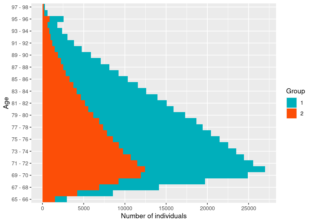
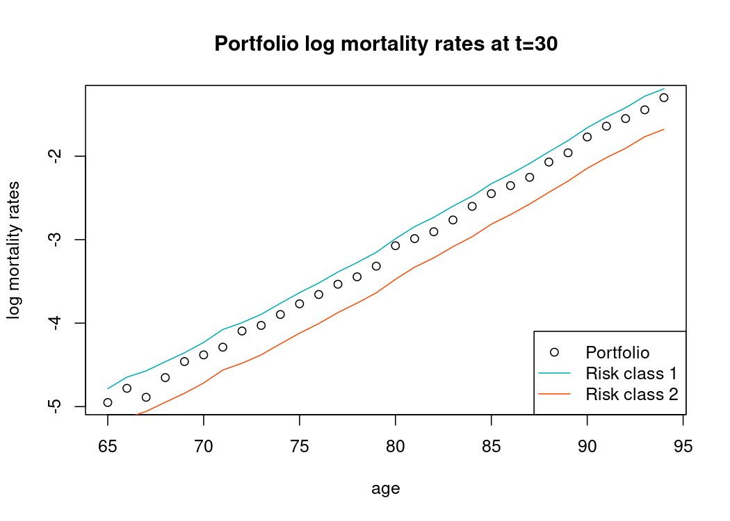
To illustrate the composition of the total population at the end of the simulation, we present in Figure 3(a) the age pyramid of the final composition of the portfolio obtained with the plot_pyramid function. In Figure 3(b), we illustrate the recalculated mortality rates using the functions death_table and mortality_table of the IBMPopSim package. Due to the mortality differential between risk class 1 and 2, one would expect to observe more individuals in risk class 2 at higher ages. However, due to exit events, a higher proportion of individuals in risk class 1 exit the portfolio over time, resulting in a greater proportion of individuals in risk class 1 at higher ages than what would be expected in the absence of exit events. Consequently, the mortality rates in the portfolio are more aligned with those of risk class 1 at higher ages.

Refer to caption
(a) Age pyramid of the individuals in the portfolio.
Refer to caption
(b) Mortality rates recalculated based on the simulated population.
Figure 3: Informations obtained from a simulation of the portfolio evolving over 30 years.

6 Population with genetically variable traits

This section provides an example of how to use the IBMPopSim package to simulate an age-structured population with genetically variable traits, based on the model proposed by [FT09].

Individuals are characterized by their body size at birth $x_{0}\in[0,4]$, which is a heritable trait subject to mutation, and by their physical age $a\in[0,2]$. The body size of an individual increases with age according to the function

$$x=x_{0}+ga,$$

where $g$ is a constant growth rate assumed to be identical for all individuals.

The birth intensity of each individual, denoted by $b(x0)$, depends on a parameter $\alpha>0$ and on their initial size, as given by the equation

$$b(x_{0})=\alpha(4-x_{0})$$ (37)

Smaller individuals have a higher birth intensity. When a birth occurs, the new individual have the same size as its parent with high probability $1-p$, or it can occur a mutation with probability $p$, resulting in a bith size given by

$$x_{0}^{\prime}=\min(\max(0,x_{0}+G),4),$$ (38)

where $G$ is a Gaussian random variable with mean 0 and variance $\sigma^{2}$.

Due to competition between individuals, the death intensity of an individual depends on the size of other individuals in the population. Bigger individuals have a better chance of survival. If an individual of size $x_{0}+ga$ encounters an individual of size $x_{0}^{\prime}+ga^{\prime}$, then it can die with the intensity

$$W(x_{0}+ga,x_{0}^{\prime}-ga^{\prime}),$$

where the interaction function $W$ is defined by

$$W(x,y)=\beta\left(1-\frac{1}{1+c\exp(-4(x-y))}\right)\in\left[0,\beta\right].$$ (39)

The death intensity of an individual of size $x0+ga$ at time $t$ is the result of interactions with all individuals in the population, including itself, and is given by

$$d(x_{0},a,t,Z_{t}^{-})=\sum_{(x_{0}^{\prime},a^{\prime})\in Z_{t}^{-}}W(x_{0}+ga,x_{0}^{\prime}+ga^{\prime}),$$

where $Z_{t}^{-}$ denotes the set of all individuals in the population at time $t$.

6.1 Population

We use an initial population of 900 living individuals, all of whom have the same size and ages uniformly distributed between 0 and 2 years.

\MakeFramed
N <- 900
x0 <- 1.06
agemin <- 0.
agemax <- 2.
\endMakeFramed
\MakeFramed
pop_init <- data.frame(
  "birth" = -runif(N, agemin, agemax), # Uniform age in [0,2]
  "death" = as.double(NA), # All individuals are alive
  "birth_size" = x0) # All individuals have the same initial birth size x0
\endMakeFramed

6.2 Events

Birth event

The parameters involved in a birth event are the probability of mutation $p$, the variance of the Gaussian random variable and the coefficient $\alpha$ of the intensity. \MakeFramed

birth_params <- list("p" = 0.03, "sigma" = sqrt(0.01), "alpha" = 1)

\endMakeFramed

The intensity of a birth event depends on the individual following (37) and is then created by calling the mk_event_individual function. The size of the new individual is given in the kernel following (38). \MakeFramed

birth_event <- mk_event_individual(
  type = "birth",
  intensity_code = "result = alpha*(4 - I.birth_size);",
  kernel_code = "if (CUnif() < p)
                   newI.birth_size = min(max(0.,CNorm(I.birth_size,sigma)),4.);
                 else
                   newI.birth_size = I.birth_size;")

\endMakeFramed
Death event

The death event depends on the interaction between individuals which is described in (39). The parameters used for this event are the growth rate $g$, the amplitude of the interaction function $\beta$, and the strength of competition $c$. The C++ code is passed as the argument interaction_code to the mk_event_interaction function. \MakeFramed

death_params <- list("g" = 1, "beta" = 2./300., "c" = 1.2)
death_event <- mk_event_interaction(
  type = "death",
  interaction_code = "double x_I = I.birth_size + g * age(I,t);
                      double x_J = J.birth_size + g * age(J,t);
                      result = beta*(1.-1./(1.+c*exp(-4.*(x_I-x_J))));")

\endMakeFramed

6.3 Model creation and simulation

To create the model, use the following code to call the function mk_model. \MakeFramed

model <- mk_model(
    characteristics = get_characteristics(pop_init),
    events = list(birth_event, death_event),
    parameters = c(params_birth, params_death))

\endMakeFramed

Before running the simulation, it is important to compute the bound $\bar{\lambda}$ for the intensity function $\lambda$ of the birth event, and the bound $\bar{W}$ for the interaction function $W$ of the intensity of the death event. In this simple model, the bounds are obvious and depend on the parameters $\alpha$ and $\beta$, more precisely we have $\bar{\lambda}=4\alpha$ and $\bar{W}=\beta$. The simulation of one scenario can then be launched with the call of the popsim function: \MakeFramed

sim_out <- popsim(model = model,
    population = pop_init,
    events_bounds = c("birth" = 4 * birth_params$alpha,
                      "death" = death_params$beta),
    parameters = c(params_birth, params_death),
    age_max = 2,
    time = 500)

\endMakeFramed

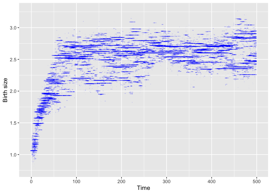
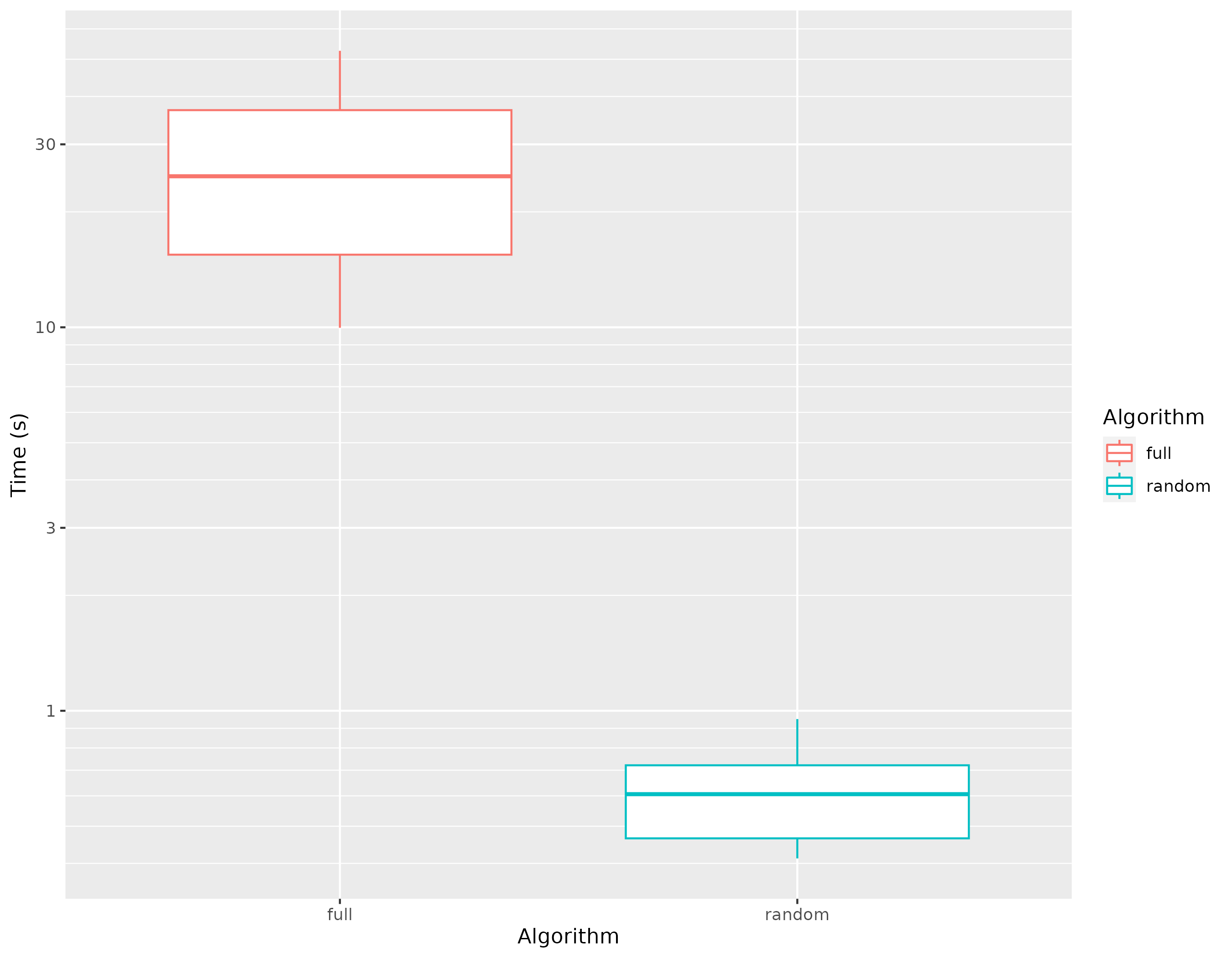
Based on the results of a simulation, we can reproduce the numerical results of [FT09]. For each individual in the population, we draw below a line representing its birth size during its life time (figure (a)). We would also like to emphasize that we have used for our simulations the randomized version of the algorithm 5, which leads to very fast computation times. Indeed, as we can see in figure (b), the computation time obtained with the random version of the algorithm is 40 times faster than the basic one, named full in the package.

Refer to caption
(a) Birth size during life time.
Refer to caption
(b) Random vs full algorithm.

Appendix A Appendix

A.1 Proof of Lemma 3.3

The proof is obtained using pathwise comparison result, generalizing those obtained in [KEK22].

Proof of Lemma 3.3.

Let $Z$ be a solution of (29). For all $e\in\mathcal{P}\cup\mathcal{E}\cup\mathcal{E}_{W}$, let $N^{e}$ be the process counting the occurrence of events of type $e$ in the population. $N^{e}$ is a counting process of $\{\mathcal{F}_{t}\}$ intensity $(\Lambda_{t}^{e}(Z_{t^{-}}))$, solution of

$\displaystyle N_{t}^{e}=\int_{0}^{t}\int_{{\mathbb{N}}\times{\mathbb{R}}^{+}}\boldsymbol{1}_{\{k\leq N_{s^{-}}\}}\boldsymbol{1}_{\{\theta\leq\lambda_{s}(I_{k},Z_{s^{-}})\}}Q(\mathrm{d}s,\mathrm{d}k,\{e\},\mathrm{d}\theta),$  $\displaystyle\quad\textit{ if }e\in\mathcal{E}\cup\mathcal{E}_{W},$
$\displaystyle N_{t}^{e}=\int_{0}^{t}\int_{{\mathbb{R}}^{+}}\boldsymbol{1}_{\{\theta\leq\mu^{e}_{t}\}}Q^{\mathcal{P}}(\mathrm{d}s,\{e\},\mathrm{d}\theta),$  $\displaystyle\quad\textit{ if }e\in\cal P.$

Furthermore, by definition the jump times of the multivariate counting process $(N^{e})_{e\in\mathcal{P}\cup\mathcal{E}\cup\mathcal{E}_{W}}$ are to the population event times $(T_{n})_{n\geq 0}$. The idea of the proof is to show that $(N^{e})_{e\in\mathcal{P}\cup\mathcal{E}\cup\mathcal{E}_{W}}$ does not explode in finite time, by pathwise domination with a simpler multivariate counting process.

Step 1 Let $(\bar{N}^{b},\bar{N}^{en})$ be the 2-dimensional counting process defined as follow. For $e=b,en$:

$\displaystyle\bar{N}_{t}^{e}=\int_{0}^{t}\int_{{\mathbb{N}}\times{\mathbb{R}}^{+}}\boldsymbol{1}_{\{k\leq N_{0}+\bar{N}_{s^{-}}\}}\boldsymbol{1}_{\{\theta\leq f^{e}(N_{0}+\bar{N}_{s^{-}})\}}Q(\mathrm{d}s,\mathrm{d}k,\{e\},\mathrm{d}\theta),\quad\textit{ if }e\in\mathcal{E}\cup\mathcal{E}_{W},$ (40)
$\displaystyle\bar{N}_{t}^{e}=\int_{0}^{t}\int_{{\mathbb{R}}^{+}}\boldsymbol{1}_{\{\theta\leq\bar{\mu}^{e}\}}Q^{\mathcal{P}}(\mathrm{d}s,\{e\},\mathrm{d}\theta)\quad\textit{ if }e\in\cal P,$

with $\bar{N}:=\bar{N}^{b}+\bar{N}^{en}$.
- If $b,en\in\cal P$, then $\bar{N}$ is a inhomogeneous Poisson process.
- If $b,en\in\mathcal{E}\cup\mathcal{E}_{W}$, then it is straightforward to show that conditionally to $N_{0}$, $\bar{N}$ is a pure birth Markov process with birth intensity function $g(n)=n\big{(}f^{b}(N_{0}+n)+f^{en}(N_{0}+n)\big{)}$. In particular, by Assumption 4, $g$ verifies the standard Feller condition for pure birth Markov processes:

$$\sum_{n=1}^{\infty}\frac{1}{g(n)},$$

(see e.g. [BM15]).
Finally, if $b\in\mathcal{E}$ and $en\in\cal P$ (or equivalently if $b\in\cal P$ and $en\in\mathcal{E}$), then one can show easily that $\bar{N}$ is a pure birth Markov process with immigration, of birth intensity function $g(n)=\bar{\mu}^{en}+nf^{b}(N_{0}+n)$ (resp. $g(n)=\bar{\mu}^{b}+nf^{en}(N_{0}+n)$), also verifying the Feller condition.

Finally, the existence of a non-exploding solution of (40) is a direct consequence of Proposition 3.3 in [KEK22].

Step 2 The second step consists in showing that $(N^{b},N^{en})$ is strongly dominated by $(\bar{N}^{b},\bar{N}^{en})$, i.e that all jumps of $(N^{b},N^{en})$ are jumps of $(\bar{N}^{b},\bar{N}^{en})$. Without loss of generality, we can assume that $f^{e}:\mathbb{N}\to\mathbb{R}^{+}$ is increasing since $f^{e}(n)$ can be replaced by $\bar{f}^{e}(n)=\sum_{m\leq n}f^{e}(m)$.
The proof is analogous to the proof of Proposition 2.1 in [KEK22].

Step 3 $e\neq b,en$: $N^{e}$ does not explode.

$$f^{e}_{t}(n)=\sup_{I\in{\mathbb{R}}\times\bar{R}\times{\mathcal{X}},m\leq n}\lambda^{e}(I,\sum_{k=1}^{m}\delta_{I_{k}}).$$

A.2 Alternative pathwise representation

Theorem A.1.

Let $\mathcal{J}_{\mathcal{E}}=\mathbb{N}\times\mathcal{E}$ and $\mathcal{J}_{W}=\mathbb{N}\times\mathcal{E}_{W}$.
Let $Q^{\mathcal{E}}$ be a random Poisson measure on $\mathbb{R}^{+}\times\mathcal{J}_{\mathcal{E}}\times\mathbb{R}^{+}$, of intensity $\mathrm{d}t\delta_{\mathcal{J}_{\mathcal{E}}}(\mathrm{d}(k,e))\mathsf{1}_{[0,\bar{\lambda}^{e}]}\mathrm{d}\theta$, and $Q^{W}$ a random Poisson measure on $\mathbb{R}^{+}\times\mathcal{J}_{W}\times\mathbb{N}\times\mathbb{R}^{+}$, of intensity $\mathrm{d}t\delta_{\mathcal{J}_{\mathcal{E}}}(\mathrm{d}(k,e))\delta_{\mathbb{N}}(\mathrm{d}j)\mathsf{1}_{[0,\bar{W}^{e}]}\mathrm{d}\theta$. Finally, let $Q^{\mathcal{P}}$ be a random Poisson measure on $\mathbb{R}^{+}\times\mathcal{P}\times[0,1]\times\mathbb{R}^{+}$, of intensity $\mathrm{d}t\delta_{\cal P}(\mathrm{d}e)\mathrm{d}u\mathsf{1}_{[0,\bar{\mu}^{e}]}(\theta)\mathrm{d}\theta$.
There exists a unique measure-valued process $Z$, strong solution on the following SDE driven by Poisson measure:

$\displaystyle Z_{t}=Z_{0}$ $\displaystyle+\int_{0}^{t}\int_{\mathcal{J}_{\mathcal{E}}\times\mathbb{R}^{+}}\phi^{e}(s,I_{k})\mathsf{1}_{\{k\leq N_{s^{-}}\}}\mathsf{1}_{\{\theta\leq\lambda_{s}^{e}(I_{k},Z_{s^{-}})\}}Q^{\mathcal{E}}(\mathrm{d}s,\mathrm{d}k,\mathrm{d}e,\mathrm{d}\theta)$
$\displaystyle+\int_{0}^{t}\int_{\mathcal{P}\times[0,1]\times\mathbb{R}^{+}}\phi^{e}(s,I_{\lfloor uN_{T_{k}}\rfloor})\mathsf{1}_{\{\theta\leq\mu_{s}^{e}\}}Q^{\mathcal{P}}(\mathrm{d}s,\mathrm{d}e,\mathrm{d}u,\mathrm{d}\theta)$
$\displaystyle+\int_{0}^{t}\int_{\mathcal{J}_{W}\times{\mathbb{N}}\times\mathbb{R}^{+}}\phi^{e}(s,I_{k})\mathsf{1}_{\{k\leq N_{s^{-}}\}}\mathsf{1}_{\{j\leq N_{s^{-}}\}}\mathsf{1}_{\{\theta\leq W^{e}(s,I_{k},I_{j})\}}Q^{W}(\mathrm{d}s,\mathrm{d}k,\mathrm{d}e,\mathrm{d}j,\mathrm{d}\theta).$ (41)

Furthermore, the solution of (A.1) has the same law than the solution of Equation (29), and Algorithm 5 is an exact simulation Equation (A.1).

References

  • [BCF+16] Sylvain Billiard, Pierre Collet, Régis Ferrière, Sylvie Méléard, and Viet Chi Tran. The effect of competition and horizontal trait inheritance on invasion, fixation, and polymorphism. Journal of theoretical biology, 411:48–58, 2016.
  • [Ben10] Harry Bensusan. Interest rate and longevity risk: dynamic model and applications to derivative products and life insurance. Theses, Ecole Polytechnique X, 2010.
  • [BM15] Vincent Bansaye and Sylvie Méléard. Stochastic Models for Structured Populations. Springer International Publishing, 2015.
  • [Bou16] Alexandre Boumezoued. Micro-macro analysis of heterogenous age-structured populations dynamics.Application to self-exciting processes and demography. Theses, Université Pierre et Marie Curie, 2016.
  • [Bré81] Pierre Brémaud. Point processes and queues: martingale dynamics, volume 66. Springer, 1981.
  • [CFM06] Nicolas Champagnat, Régis Ferrière, and Sylvie Méléard. Unifying evolutionary dynamics: from individual stochastic processes to macroscopic models. Theoretical population biology, 69(3):297–321, 2006.
  • [CHLM16] Manon Costa, Céline Hauzy, Nicolas Loeuille, and Sylvie Méléard. Stochastic eco-evolutionary model of a prey-predator community. Journal of mathematical biology, 72:573–622, 2016.
  • [CIH+20] Vincent Calvez, Susely Figueroa Iglesias, Hélène Hivert, Sylvie Méléard, Anna Melnykova, and Samuel Nordmann. Horizontal gene transfer: numerical comparison between stochastic and deterministic approaches. ESAIM: Proceedings and Surveys, 67:135–160, 2020.
  • [Çin11] Erhan Çinlar. Probability and Stochastics. Springer New York, 2011.
  • [CMM13] Pierre Collet, Sylvie Méléard, and Johan AJ Metz. A rigorous model study of the adaptive dynamics of mendelian diploids. Journal of Mathematical Biology, 67:569–607, 2013.
  • [Dev86] Luc Devroye. Nonuniform random variate generation. Springer-Verlag, New York, 1986.
  • [EHK21] Nicole El Karoui, Kaouther Hadji, and Sarah Kaakai. Simulating long-term impacts of mortality shocks: learning from the cholera pandemic. arXiv preprint arXiv:2111.08338, 2021.
  • [FM04] Nicolas Fournier and Sylvie Méléard. A microscopic probabilistic description of a locally regulated population and macroscopic approximations. Ann. Appl. Probab., 14(4):1880–1919, 2004.
  • [FT09] Régis Ferrière and Viet Chi Tran. Stochastic and deterministic models for age-structured populations with genetically variable traits. volume 27 of ESAIM Proc., pages 289–310. EDP Sci., Les Ulis, 2009.
  • [Kal17] Olav Kallenberg. Random measures, theory and applications, volume 77 of Probability Theory and Stochastic Modelling. Springer, Cham, 2017.
  • [KEK22] Sarah Kaakai and Nicole El Karoui. Birth death swap population in random environment and aggregation with two timescales. arXiv preprint arXiv:1803.00790, 2022.
  • [LS79] Peter Lewis and Gerald Shedler. Simulation of nonhomogeneous poisson processes by thinning. Naval research logistics quarterly, 26(3):403–413, 1979.
  • [LSA+19] François Lavallée, Charline Smadi, Isabelle Alvarez, Björn Reineking, François-Marie Martin, Fanny Dommanget, and Sophie Martin. A stochastic individual-based model for the growth of a stand of japanese knotweed including mowing as a management technique. Ecological Modelling, 413:108828, 2019.
  • [MRR19] Sylvie Méléard, Michael Rera, and Tristan Roget. A birth–death model of ageing: from individual-based dynamics to evolutive differential inclusions. Journal of mathematical biology, 79:901–939, 2019.
  • [RJMR22] Tristan Roget, Pierre Jolivet, Sylvie Méléard, and Michael Rera. Positive selection of senescence through increased evolvability: ageing is not a by-product of evolution. bioRxiv, pages 2022–03, 2022.
  • [Tra06] Viet Chi Tran. Modèles particulaires stochastiques pour des problèmes d’évolution adaptative et pour l’approximation de solutions statistiques. Theses, Université de Nanterre - Paris X, 2006.
  • [Tra08] Viet Chi Tran. Large population limit and time behaviour of a stochastic particle model describing an age-structured population. ESAIM: Probability and Statistics, 12:345–386, 2008.
  • [VKM18] Andrés M. Villegas, Vladimir K. Kaishev, and Pietro Millossovich. StMoMo: An R Package for Stochastic Mortality Modelling. Journal of Statistical Software, 84:1–38, 2018.
  • [Zin14] Sabine Zinn. The MicSim package of R: an entry-level toolkit for continuous-time microsimulation. International Journal of Microsimulation, 7(3):3–32, 2014.