Efficient Spin-Orbit Torque in Antiferromagnetic Topological Insulator MnBi₂Te₄

Abstract

We formulate and quantify the spin-orbit torque (SOT) in intrinsic antiferromagnetic topological insulator $\rm MnBi_{2}Te_{4}$ of a few septuple-layer thick, which exhibits conspicuous layer-resolved characteristics. Contrary to known current-induced torques, the SOT in insulating $\rm MnBi_{2}Te_{4}$ is driven by an electric field (or voltage). We further study the SOT-induced magnetic resonances, where in the tri-septuple-layer case we identify a peculiar exchange mode that is blind to microwaves but can be exclusively driven by the predicted SOT. As an inverse effect of the SOT, topological charge pumping generates an adiabatic current devoid of Joule heating, which occurs concomitantly with the SOT and gives rise to an overall magneto-reactance for $\rm MnBi_{2}Te_{4}$, enabling a lossless conversion of electric power into magnetic dynamics.

Achieving efficient control of magnetism and magnetic dynamics via electrical means has been a central inquiry in modern spintronics [1, 2, 3, 4]. At present, such control can be typically realized in an engineered heterostructure consisting of a magnetic layer and a heavy metal layer converting electric driving forces into spin angular momenta [5, 6, 7, 8, 9, 10, 11, 12]. However, the spatial separation of electric and magnetic components in such a heterostructure fundamentally restricts its operational efficiency owing to non-local spin diffusion, hindered interfacial spin transmission, and other undesired complications associated with the interface.

The advent of 2D magnetic materials opens up new physical scenarios for spintronics such that spin angular momenta can be generated and delivered locally inside the same material, enabling direct control of magnetic states through electric stimuli in the absence of engineered interfaces [13, 14, 15, 16]. Therefore, as long as it affords strong spin-orbit interactions, a 2D magnet on its own could simultaneously play the roles of two distinct layers of a 3D heterostructure. However, little is known about the specific form of electrical manipulation of magnetic states and its governing mechanism in 2D magnets without resorting to foreign spin generators, as the established models based on 3D heterostructures are largely invalid in reduced dimensions.

Recent studies identified $\rm MnBi_{2}Te_{4}$ as an intrinsic 2D antiferromagnetic (AFM) topological insulator featuring layer-dependent magnetic order intertwined with the non-trivial topology of electronic bands [17, 18, 19, 20, 21, 22, 23, 24, 25], which provides an excellent testing ground for the electrical manipulation of magnetic states in 2D magnets. In particular, it is tempting to ask if the layered AFM order of $\rm MnBi_{2}Te_{4}$ can be driven by an applied electric field by virtue of the strong spin-orbit coupling in the material.

In this Letter, we formulate and quantify the spin-orbit torque (SOT) driven by an in-plane applied electric field and its inverse effect, dubbed topological charge pumping, in $\rm MnBi_{2}Te_{4}$ of a few septuple-layer (SL) thick using the effective Lagrangian approach. The SOT is manifestly SL-resolved and displays an evident even-odd SL-number pattern, echoing the even-odd distinction of the electronic states widely reported in previous studies [19, 25, 26]. The physical consequences of the SOT are demonstrated by the SOT-induced magnetic resonances in 2-SL and 3-SL $\rm MnBi_{2}Te_{4}$ samples, where in the 3-SL case we identify a unique exchange mode that is blind to microwave electromagnetic fields but can be excited only by the SL-resolved SOT. Guided by symmetry considerations, we also generalize the SOT into systems of more SLs, where the even-odd pattern persists.

Contrary to traditional current-induced torques, the SOT we study in $\rm MnBi_{2}Te_{4}$ arises from the applied electric field (or voltage) as the Fermi level lies in the gap. The output current is purely adiabatic and does not incur Joule heating; it is produced by the coherent dynamics of the AFM order rather than Ohm’s conduction [besides the dissipationless quantum anomalous Hall (QAH) current]. Accounting for the combined action of the SOT and topological charge pumping, a voltage-driven $\rm MnBi_{2}Te_{4}$ acquires an effective magneto-reactance, whereby $100\%$ of the input power can be converted into magnetic dynamics to overcome the Gilbert damping, realizing a remarkably high efficiency in the electric control of magnetism in a single 2D material.

Formalism.—We start by constructing an effective Lagrangian density to quantify the dynamics of a semiclassical wavepacket $\ket{W}$ for a Bloch electron with the center-of-mass position $\bm{r}_{c}=\bra{W}\hat{\bm{r}}\ket{W}$ and momentum $\bm{k}_{c}=\bra{W}\hat{\bm{k}}\ket{W}$ [27], whose spin couples the unit magnetization vector $\bm{m}^{j}$ ($j$ is the SL index) through the exchange interaction. To simplify our notation, we focus on a single energy band well-separated from all other bands, which is non-degenerate (doubly degenerate) for an odd (even) total number of SLs. The Lagrangian density of such a wavepacket perturbed by electromagnetic fields expressed in vector potential $\mathscr{\bm{A}}$ and scalar potential $\varphi$ can be written as

$$\mathscr{L}_{em}= \hbar\dot{\bm{r}}_{c}\cdot(\bm{k}_{c}-e\mathscr{\bm{A}})-\epsilon(\bm{k}_{c})$$

$$+\hbar\eta^{\dagger}\left(\mathrm{i}\frac{d}{dt}+\bm{A}^{k}\cdot\dot{\bm{k}}_{c}+\bm{A}^{m^{j}}\cdot\dot{\bm{m}}^{j}\right)\eta$$ (1)

where $\hbar$ is the reduced Planck constant, $e>0$ is the absolute electron charge, and summations of repeated indices are assumed (here and hereafter). For a non-degenerate band, $\eta=1$. For a degenerate band, $\eta$ becomes a column vector specifying the projection of the wavepacket on each sub-band [28]: $\ket{W}=\int d\bm{k}w(\bm{k})e^{\mathrm{i}\bm{k}\cdot\bm{r}}\eta_{a}\ket{u_{a}}$ where $\ket{u_{a}}$ is the periodic part of the Bloch wavefunction and the spectral profile function $w(\bm{k})$ satisfies $\int d\bm{k}|w(\bm{k})|^{2}\bm{k}=\bm{k}_{c}$. The interplay between the electron and the SL magnetization is characterized by the Berry connection matrices: $[A_{ab}]^{\alpha}_{\mu}\equiv\mathrm{i}\bra{u_{a}}\partial^{\alpha}_{\mu}\ket{u_{b}}$, where $\partial_{\mu}^{\alpha}$ stands for $\partial/\partial k_{\mu}$ when $\alpha=k$ and $\partial/\partial m^{j}_{\mu}$ when $\alpha=m^{j}$. In Eq. (1), the band energy of the wavepacket is $\epsilon(\bm{k}_{c})=\bra{W}H\ket{W}$, where $H=H_{0}(\hbar\bm{k}+e\bm{\mathscr{A}})-e\varphi$ with $H_{0}(\bm{\mathscr{A}}\rightarrow 0)$ being the unperturbed Hamiltonian. The spatial variation of $\bm{m}^{j}$ in the lateral (in-plane) dimensions is ignored, otherwise the real-space Berry connection $\bm{A}^{r}$ will also be present.

The Lagrangian density for the dynamics of $\bm{m}^{j}$ is $\mathscr{L}_{m^{j}}=\hbar S(1-\cos\theta^{j})\partial_{t}\phi^{j}-\mathscr{H}^{j}$ [29], where $\theta^{j}$ and $\phi^{j}$ are the spherical angles specifying the direction of $\bm{m}^{j}$, $S$ is the total spin quantum number (of a unit cell in each SL), and $\mathscr{H}^{j}$ is the magnetic free energy of $\bm{m}^{j}$ including the inter-SL exchange coupling and the magnetic anisotropy. Applying the Euler-Lagrangian equation on $\mathscr{L}_{tot}=\mathscr{L}_{em}+\sum_{j}\mathscr{L}_{m^{j}}$, followed by an integration of $\bm{k}_{c}$ over the first Brillouin zone, we obtain the Landau-Lifshitz-Gilbert (LLG) equation for $\bm{m}^{j}$ and the in-plane current density as [30]

$$\dot{\bm{m}}^{j} =\gamma(\bm{H}^{\rm eff}_{j}+\bm{H}_{j}^{\rm T})\times\bm{m}^{j}+\alpha_{\rm G}\bm{m}^{j}\times\dot{\bm{m}}^{j},$$ (2a)

$$\bm{J} =\sigma_{0}\bm{E}+\sigma_{\rm AH}\hat{\bm{z}}\times\bm{E}+\bm{J}^{\rm p},$$ (2b)

where $\sigma_{0}$ and $\sigma_{\rm AH}$ are the longitudinal and QAH components of conductivity, $\hat{\bm{z}}$ is the unit vector normal to the plane, $\bm{E}=-\bm{\nabla}\varphi-\partial_{t}\mathscr{\bm{A}}$ is the applied electric field, $\bm{H}^{\rm eff}_{j}=(-1/\hbar\gamma S)\partial(\sum_{i}\mathscr{H}^{i})/\partial\bm{m}^{j}$ (with $\gamma$ the gyro-magnetic ratio) is the effective magnetic field acting on $\bm{m}^{j}$ in the absence of electric stimuli, and $\alpha_{\rm G}$ is the Gilbert damping constant. In Eqs. (2a) and (2b), $\bm{H}_{j}^{\rm T}$ is the effective field of the voltage-induced SOT and $\bm{J}^{\rm p}$ is the current density generated by topological charge pumping. In the Cartesian coordinates,

$${H}_{j,\mu}^{\rm T} =\frac{ea_{0}^{2}}{\gamma\hbar S}\int\frac{{\rm d}^{2}k}{(2\pi)^{2}}f(\bm{k}){\rm{Tr}}(\Omega^{km^{j}}_{\nu\mu})E_{\nu},$$ (3a)

$$J^{\rm p}_{\mu} =-e\int\frac{{\rm d}^{2}k}{(2\pi)^{2}}f(\bm{k}){\rm{Tr}}(\Omega^{m^{j}k}_{\nu\mu})\dot{m}^{j}_{\nu},$$ (3b)

where $a_{0}$ is the lattice constant, $f(\bm{k})$ is the Fermi-Dirac distribution function, and $\Omega^{\alpha\beta}_{\mu\nu}=\partial^{\alpha}_{\mu}A^{\beta}_{\nu}-\partial^{\beta}_{\nu}A^{\alpha}_{\mu}-\mathrm{i}[A^{\alpha}_{\mu},A^{\beta}_{\nu}]$ is the Berry curvature tensor in which the commutation term will vanish identically if bands are non-degenerate (for an odd total number of SLs). In Eq. (3), the trace is taken in the degenerate subspace (for an even total number of SLs), which results from thermal averaging of the inter-sub-bands transitions embedded in the dynamics of $\eta$ [31].

Without doping or gating, $\rm MnBi_{2}Te_{4}$ is insulating regardless of the number of SLs, so $\sigma_{0}$ always vanishes. On the other hand, $\sigma_{\rm AH}$ is quantized for odd-SL samples and zero for even-SL samples, as it arises from the momentum-space Berry curvature $\Omega_{\mu\nu}^{kk}$. By contrast, $\bm{J}^{\rm p}$ and $\bm{H}_{j}^{\rm T}$ originate from the Berry curvature $\Omega_{\mu\nu}^{km}$ lying in the mixed space spanned by the crystal momentum and the magnetization vector.

Voltage-induced SOT.—We next calculate the field of SOT according to Eq. (3a) for different thicknesses. To this end, we need to construct the unperturbed electron Hamiltonian $H_{0}(\bm{k})$ in terms of the SL-specific Hamiltonian $h_{j}$ and the inter-SL hopping $T_{ij}$, both of which could be obtained by discretizing the bulk Hamiltonian in the vertical dimension [20, 32, 33]. Under the basis $[\ket{p_{z,\rm Bi}^{+},\uparrow},\ket{p_{z,\rm Te}^{-},\uparrow},\ket{p_{z,\rm Bi}^{+},\downarrow},\ket{p_{z,\rm Te}^{-},\downarrow}]^{T}$,

$$h_{j}(\bm{k}) =\epsilon(\bm{k})+d_{a}(\bm{k})\Gamma_{a}+\gamma_{\rm ex}\bm{m}^{j}\cdot\bm{\sigma}\otimes(\tau_{0}+\delta\tau_{3}),$$ (4a)

$$T_{ij} =\sigma_{0}\otimes(D_{1}\tau_{0}+B_{1}\tau_{3})+\mathrm{i}A_{1}\sigma_{z}\otimes\tau_{1},$$ (4b)

where $\epsilon(\bm{k})=C+2D_{1}+D_{2}(k_{x}^{2}+k_{y}^{2})$, $d_{0}(\bm{k})=M_{0}+2B_{1}+B_{2}(k^{2}_{x}+k^{2}_{y})$, $d_{1(2)}(\bm{k})=A_{2}k_{x(y)}$, $\gamma_{\rm ex}$ is the exchange coupling, $\Gamma_{0}=\sigma_{0}\otimes\tau_{3}$, and $\Gamma_{1(2)}=\sigma_{1(2)}\otimes\tau_{1}$ with $\sigma$ and $\tau$ the Pauli matrices in the spin and orbital spaces. A bias term $\delta\tau_{3}$ is included in Eq. (4a) to account for the asymmetric exchange coupling for the $p$-orbitals of the Bi and Te atoms. The values of $\delta$, $M_{0}$, $A_{1(2)}$, $B_{1(2)}$ $C$, $D_{1(2)}$ are detailed in [30]. The following discussions will be restricted to the low-temperature regime such that $f(\bm{k})\approx 1$ for $\epsilon(\bm{k})$ below the Fermi level $\epsilon_{F}$ and $f(\bm{k})\approx 0$ otherwise.

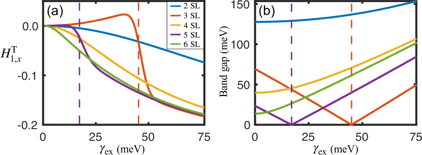
Figure 1: (a) The effective field of SOT acting on the bottom SL and (b) the band gap at the $\Gamma$ point as functions of $\gamma_{\rm ex}$ from 2 to 6 SLs. $H^{\rm T}_{1,x}$ is plotted in unit of $eEa_{0}/4\pi^{2}\hbar\gamma S$.

Without loss of generality, we set $\bm{E}=E\hat{\bm{x}}$ so the ${\rm{Tr}}(\Omega_{\nu\mu}^{km^{j}})$ tensor reduces to a vector, whose direction corresponds to that of $\bm{H}^{T}_{j}$ according to Eq. (3a). Numerically, we find that $\bm{H}^{T}_{j}$ is in the $x$ direction (collinear with $\bm{E}$) with its amplitude maximized on the outermost SLs. Figure 1(a) plots $H_{1,x}^{\rm T}$ (acting on the bottom SL) as a function of the exchange coupling $\gamma_{\rm ex}$ for the AFM configuration, $\bm{m}^{j}=(-1)^{j+1}\hat{\bm{z}}$, from 2 to 6 SL thick. We have excluded the 1-SL case in which the SOT vanishes identically. For any inner SL, $H_{j,x}^{\rm T}$ is substantially weaker than $H_{1,x}^{\rm T}$ but its variation with $\gamma_{\rm ex}$ is similar [30]. In the odd-SL cases $H_{1,x}^{\rm T}$ changes non-monotonically with a sharp turn (marked by dashed line) whereas in the even-SL cases it varies monotonically. To demystify this striking contrast between even and odd systems, we plot in Fig. 1(b) the $\Gamma$-point band gap versus $\gamma_{\rm ex}$ for corresponding SLs, where it is evident that the gap closes at the sharp turn of $H_{1,x}^{\rm T}$. We also inspected the total Chern number $C$ of the bands below $\epsilon_{F}$, which transitions from $0$ to $-1$ across the gap-closing point for the odd-SL cases while remaining to be $0$ for the even-SL cases. This observation implies that a non-zero SOT is not necessarily related to a non-trivial band topology, at least for the even-SL cases. Even for an odd-SL $\rm MnBi_{2}Te_{4}$, the SOT turns out to be finite in the $C=0$ phase although it is much stronger in the $C=-1$ phase. An intuitive understanding is that the exchange imbalance $\delta$ serves as an effective spin-orbit coupling, giving rise to a non-zero SOT even when the electron bands are topologically trivial.

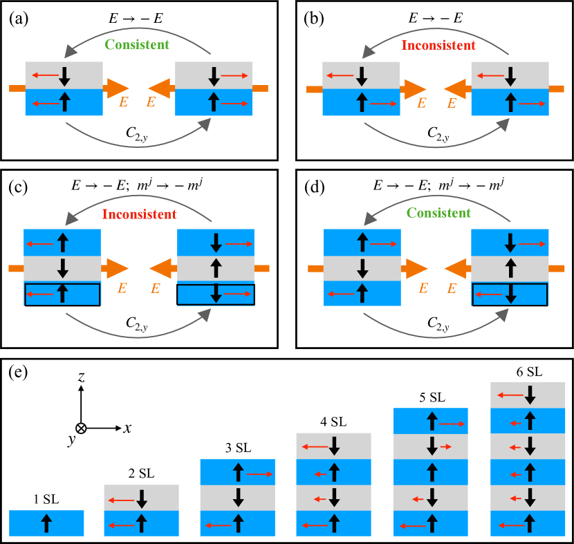
Figure 2: (a)-(d) Symmetry analysis of the SL-resolved SOT fields (red arrows) for 2-SL and 3-SL $\rm MnBi_{2}Te_{4}$. $C_{2,y}$ denotes the two-fold rotation around the $y$ axis. (e) SOT fields from 1 SL to 6 SL.

The SOT displays an interesting SL-resolved pattern. In a 2-SL sample the field of SOT is the same for both SLs, $H_{1,x}^{\rm T}=H_{2,x}^{\rm T}$, while in a 3-SL sample, $H_{1,x}^{\rm T}=-H_{3,x}^{\rm T}$ and $H_{2,x}^{\rm T}=0$. As illustrated in Fig. 2(a)–(d), this pattern is ensured by the symmetry of the system. For example, a two-fold rotation around the $y$ axis (denoted by $C_{2,y}$) in a 2-SL system amounts to flipping the direction of $\bm{E}$ while leaving the magnetic configuration and the atomic structure unchanged, which should lead to a simple sign change of $\bm{H}_{j}^{\rm T}$. Therefore, the system returns to itself under the combined operation of $C_{2,y}$ and $\bm{E}\rightarrow-\bm{E}$ (and they are interchangeable). To make it clearer, we illustrate in Fig. 2(b) why an antisymmetric pattern $H_{1,x}^{\rm T}=-H_{2,x}^{\rm T}$ is inconsistent with the linear response regime (i.e., $\bm{H}_{j}^{\rm T}$ flips sign when $\bm{E}$ reverses). Similarly, the $C_{2,y}$ operation on a 3-SL system flips not only the $\bm{E}$ field but also the magnetization in all SLs, thus an identity operation combines $C_{2,y}$, $\bm{E}\rightarrow-\bm{E}$, and $\bm{m}^{j}\rightarrow-\bm{m}^{j}$. Consequently, a 3-SL system driven by $\bm{E}=E\hat{\bm{x}}$ is consistent only when $H_{j,x}^{\rm T}$ is strictly antisymmetric among the constituent SLs, which is demonstrated in Fig. 2(c) and (d). The symmetry argument can be generalized into more SLs. As shown in Fig. 2(e), the SOT field is indeed symmetrically (antisymmetrically) distributed among the SLs in an even-SL (odd-SL) sample. For the odd-SL cases, the SOT exerting on the middle SL must vanish in order to respect the symmetry requirement, which naturally explains why the SOT is identically zero in the case of 1-SL. It should be noted that the red arrows indicating $\bm{H}_{j}^{\rm T}$ are drawn for illustration only; their exact magnitudes are detailed in [30].

Driven by the SOT, an $\rm MnBi_{2}Te_{4}$ will deviate from its AFM ground state, which in turn affects the exchange coupling $\bm{m}^{j}\cdot\bm{\sigma}$ in Eq. (4a) and changes the SOT. Therefore, to solve the SOT-driven magnetic dynamics in a closed form, it is necessary to determine the SOT field under all possible magnetic configurations. However, in a multi-SL system, this will involve too many variables to implement numerically. A practical strategy is to identify experimentally relevant dynamics, such as resonance modes, and then study the SOT for a particular configuration associated with a selected eigenmode.

Magnetic resonances.—The SOT can be verified and characterized experimentally via SOT-induced magnetic resonances. In light of the symmetry features discussed above, we study the magnetic resonances in the 2-SL and 3-SL cases driven by an in-plane ac electric field $\tilde{E}e^{\mathrm{i}\omega t}$ (phasor form adopted hereafter), which exemplifies the anticipated even-odd contrast. Within the macrospin description, a 2-SL $\rm MnBi_{2}Te_{4}$ can be modeled as a collinear two-sublattice antiferromagnet. As plotted in Fig. 3(a), the resonance frequencies are $\omega^{r}_{1(2)}=\sqrt{\omega_{A}(2\omega_{E}+\omega_{A})}\pm\omega_{0}$ [34], where $\omega_{E}$ is the inter-SL Heisenberg exchange interaction expressed in angular frequency, $\omega_{A}$ is the perpendicular easy-axis anisotropy, and $\omega_{0}=\gamma H_{0}$ is the bias magnetic field in the $z$ direction. The corresponding eigenmodes are circularly polarized, exhibiting opposite chirality as illustrated in Fig. 3(b). Since the instantaneous SOT field is the same for both SLs [Fig. 2(a)], $\tilde{E}e^{\mathrm{i}\omega t}$ drives the 2-SL system like a microwave. Consequently, the dynamical susceptibility as a function of $\omega$ should assume the same form as that of microwave-driven AFM resonance. Besides the SOT field, the electric drive $\tilde{E}e^{\mathrm{i}\omega t}$ also generates an Oersted field in the transverse direction through the displacement current (Ohm’s current is zero) and an SL-independent longitudinal magnetic field through the topological magnetoelectric effect (unique to axion insulators), but both effects turn out to be negligible [30].

The 3-SL case is quite non-trivial. In the absence of SOT, solving a set of coupled LLG equations for the SL-specific magnetization gives three distinct resonance modes [30]

$$\omega^{r}_{1} =\sqrt{\omega_{A}^{2}+3\omega_{A}\omega_{E}+\frac{\omega_{E}^{2}}{4}}-\frac{\omega_{E}}{2}+\omega_{0},$$ (5a)

$$\omega^{r}_{2} =\sqrt{\omega_{A}^{2}+3\omega_{A}\omega_{E}+\frac{\omega_{E}^{2}}{4}}+\frac{\omega_{E}}{2}-\omega_{0},$$ (5b)

$$\omega^{r}_{3} =\omega_{A}+\omega_{E}+\omega_{0},$$ (5c)

which are plotted in Fig. 3(c). The SL-specific motions for each mode are illustrated in Fig. 3(d). The right-handed mode $\omega_{1}^{r}$ (blue) and the left-handed mode $\omega_{2}^{r}$ (red), while having counterparts in the 2-SL case, are non-degenerate at zero field, which can be attributed to the uncompensated magnetization in the ground state that explicitly breaks the $C_{2,y}$ symmetry. In addition, we identify an exotic right-handed mode $\omega_{3}^{r}$ (green) in which the top and bottom SLs precess out-of-phase while the middle SL stays stationary as the instantaneous exchange torque exerting on it by the neighboring SLs exactly cancel. Even though the top and bottom SLs do not directly couple, they strongly affect each other through the middle SL thanks to the inter-SL Heisenberg exchange interaction $\omega_{E}$, thus the $\omega_{3}^{r}$ mode can be regarded as a special exchange mode.

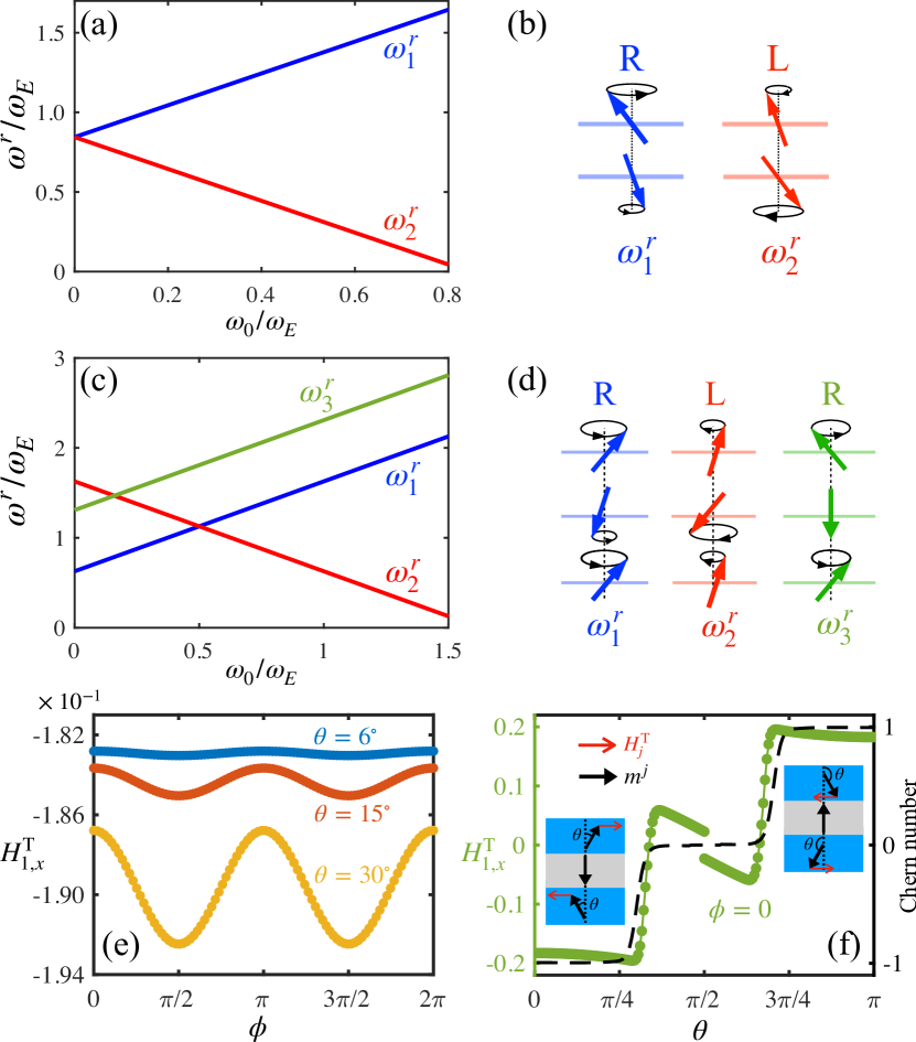
Figure 3: Resonance frequencies varying with a bias magnetic field applied in the $\hat{z}$ direction (scaled into angular frequency $\omega_{0}$ and is relative to $\omega_{E}$) for (a) 2-SL and (c) 3-SL $\rm MnBi_{2}Te_{4}$. (b) and (d) illustrate the SL-specific magnetic precessions in each resonance eigenmode. The strength of SOT field under the $\omega_{3}^{r}$ configuration: (e) as a function of $\phi$ for different $\theta$; (f) as a function of $\theta$ for $\phi=0$, where the total Chern number is also shown (dashed curve). $\bm{m}^{2}$ is opposite for $\theta\in[0,\pi/2)$ and $(\pi/2,\pi]$ to ensure the $\omega_{3}^{r}$ configuration. Parameters: $\gamma_{\rm ex}=75\ \rm meV$, $\hbar\omega_{E}=0.272\ \rm meV$ and $\hbar\omega_{A}=0.084\ \rm meV$ [25].

Leveraging the $\omega_{3}^{r}$ mode calls for a staggered ac field acting oppositely on the top and bottom SLs while leaving the middle SL unperturbed, which coincides with the SL-contrasting SOT field depicted in Fig. 2(d). Therefore, we anticipate that by exploiting the voltage-induced SOT, an in-plane electric field drive $\tilde{E}e^{\mathrm{i}\omega t}$ is able to induce the resonance of the $\omega_{3}^{r}$ mode. On the other hand, this mode is blind to a microwave because at the resonance frequency its wavelength far exceeds the SL spacing so that the oscillating field is SL independent. Moreover, even though the Oersted field arising from $\tilde{E}e^{\mathrm{i}\omega t}$ is also staggered, it is much weaker than the SOT field [30]. Consequently, observing the resonance of the $\omega_{3}^{r}$ mode provides an unequivocal way to verify the SOT.

To determine if the symmetry pattern of SOT illustrated in Fig. 2(d) persists for large-angle precessions, we numerically compute $\bm{H}_{j}^{\rm T}$ for arbitrary amplitudes of excitation of the $\omega_{3}^{r}$ mode. We find that $\bm{H}_{2}^{\rm T}=0$ and $H_{1,x}^{\rm T}=-H_{3,x}^{\rm T}$ (the $y$, $z$ components vanish) always hold. Figure 3(e) plots $H_{1,x}^{\rm T}$ as a function of the azimuthal angle $\phi$ for different polar angles, which oscillates within a narrow range of values and can thus be approximated as independent of $\phi$. Figure 3(f) plots $H_{1,x}^{\rm T}$ as a function of the polar angle $\theta$ at $\phi=0$, where sharp turns appear around $\theta\approx\pi/3$ and $2\pi/3$. We also plot in Fig. 3(f) the total Chern number varying over $\theta$, which indicates that the electronic structure undergoes topological phase transitions at where $H_{1,x}^{\rm T}$ changes sharply. We mention that our formalism breaks down in the vicinity of these transitions where the bands close at the $\Gamma$ point and the adiabatic condition is violated. So rigorously speaking, $H_{1,x}^{\rm T}$ should jump abruptly at the sharp turns, whereas the appearing continuity in Fig. 3(f) is ascribed to numerical errors.

Basing on the above observation, we can approximate the SOT field acting on each SL as a constant up to $\theta\approx\pi/3$ without worrying about gap closing. By including the ac SOT field into the linearized LLG equations using phasor notations, we can solve the dynamical susceptibility as $\tilde{\chi}_{\parallel}=\tilde{m}^{1}_{x}/\gamma\tilde{H}^{\rm T}_{1,x}=\tilde{m}^{3}_{x}/\gamma\tilde{H}^{\rm T}_{3,x}$ and $\tilde{\chi}_{\perp}=\tilde{m}^{1}_{y}/\gamma\tilde{H}^{\rm T}_{1,x}=\tilde{m}^{3}_{y}/\gamma\tilde{H}^{\rm T}_{3,x}$ [30]:

$$\tilde{\chi}_{\parallel}(\omega)=\frac{-(\mathrm{i}\alpha_{\rm G}\omega+\omega_{3}^{r})}{\omega^{2}-(\mathrm{i}\alpha_{\rm G}\omega+\omega_{3}^{r})^{2}},$$ (6a)

$$\tilde{\chi}_{\perp}(\omega)=\frac{\mathrm{i}\omega}{\omega^{2}-(\mathrm{i}\alpha_{\rm G}\omega+\omega_{3}^{r})^{2}}.$$ (6b)

The dynamical susceptibility thus define cannot be measured directly because the oscillating SOT field is an intermediate quantity generated by $\tilde{E}e^{\mathrm{i}\omega t}$—the true driving force. To detect the SOT-induced resonance electronically, we must consider the inverse effect of the SOT to eliminate the magnetic degrees of freedom, which brings us to the next topic.

Topological charge pumping.—As the SL-dependent magnetization is driven into motion, the precessing magnetic moments will generate an adiabatic current according to Eq. (3b), which is the reciprocal effect of SOT commonly known as topological charge pumping [35, 36]. In contrast to transport currents, an adiabatic current is not accompanied by Joule heating (i.e., it is non-dissipative) and it decays rapidly when the system goes off-resonance [37, 38, 39]. Therefore, in a pure voltage-driven system, the pumped adiabatic current $\bm{J}^{\rm p}$ directly signals the onset of magnetic resonances. The overall effect combining the voltage-induced SOT, LLG equations, and topological charge pumping manifests as a linear response relation: $\tilde{J}_{\mu}^{\rm P}(\omega)=\tilde{\sigma}_{\mu\nu}(\omega)\tilde{E}_{\nu}(\omega)$. For the 3-SL case, the ac conductivity (or electric admittance) tensor includes

$$\tilde{\sigma}_{xx}(\omega) =\mathrm{i}\omega\tilde{\chi}_{\parallel}(\omega)\frac{2e^{2}a_{0}^{2}}{\hbar S}\left\langle{\rm Tr}(\Omega_{xx}^{km^{1}})\right\rangle^{2},$$ (7a)

$$\tilde{\sigma}_{yx}(\omega) =\mathrm{i}\omega\tilde{\chi}_{\perp}(\omega)\frac{2e^{2}a_{0}^{2}}{\hbar S}\left\langle{\rm Tr}(\Omega_{yy}^{km^{1}})\right\rangle^{2},$$ (7b)

where $\langle(\cdots)\rangle=1/(2\pi)^{2}\int{\rm d}^{2}kf(\bm{k})(\cdots)$ denotes the average over the first Brillouin zone [30]. We plot the amplitude and phase of $\tilde{\sigma}_{xx}$ and $\tilde{\sigma}_{yx}$ as functions of the driving frequency $f=\omega/2\pi$ in Fig. 4(a) and (b), respectively. It is obvious that the amplitude $|\tilde{\chi}_{\parallel(\perp)}(\omega)|$ only has a single peak at $\omega_{3}^{r}$ [which can be seen also from Eqs. (6a) and (6b)], indicating that the SOT exclusively excites the $\omega_{3}^{r}$ mode; it does not excite the $\omega_{1}^{r}$ and $\omega_{2}^{r}$ modes (the ordinary AFM resonances) at all [40]. On the contrary, a microwave source can only drive the $\omega_{1}^{r}$ and $\omega_{2}^{r}$ modes but not $\omega_{3}^{r}$ (see Fig. S5 [30] for details). This contrasting feature confirms our expectation based on the symmetry of SOT shown in Fig. 2. Furthermore, both $\tilde{\sigma}_{xx}$ and $\tilde{\sigma}_{yx}$ change the phase by $\pi$ across the resonance of $\omega_{3}^{r}$, but their relative phase is always $\pi/2$. From the ac conductivity, we can tell that the system behaves as an insulator when the resonance is off while it conducts pure adiabatic current (dissipationless) when the resonance is on, which is very straightforward to detect electronically [39].

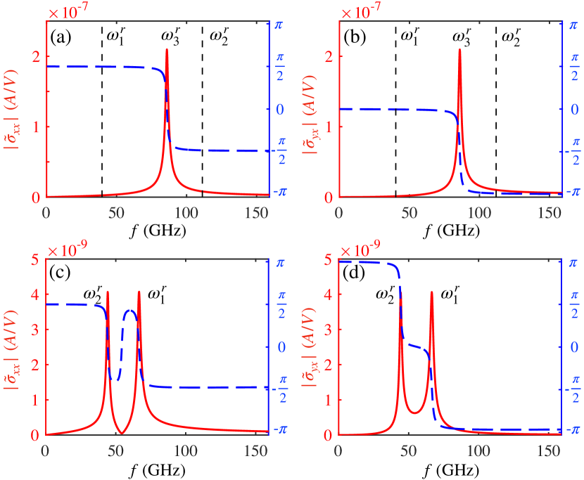
Figure 4: Amplitude (solid red) and phase (dashed blue) of $\tilde{\sigma}_{xx}$ and $\tilde{\sigma}_{yx}$ as functions of $f=\omega/2\pi$. (a) and (b) for 3-SL and (c) and (d) for 2-SL $\rm MnBi_{2}Te_{4}$. $\omega_{l}^{r}$ refers to the $l$-th resonance mode. Parameters: $\alpha_{\rm G}=0.01$ (damping), $\hbar\omega_{0}=0.046$ meV (bias field, for 2-SL only), and the rest are the same as those used in plotting Fig. 3.

As a comparison, we also plot $\tilde{\sigma}_{xx}$ and $\tilde{\sigma}_{yx}$ associated with a 2-SL $\rm MnBi_{2}Te_{4}$ in Figs. 4(c) and (d), where a perpendicular bias magnetic field of $\hbar\omega_{0}=0.046$ meV (about $0.4$ T) is applied to break the degeneracy of $\omega_{1}^{r}$ and $\omega_{2}^{r}$ [see Fig. 3(a)]. In stark contrast to the 3-SL case, the ac conductivity now exhibits peaks at both chiral modes of the AFM resonances, because the symmetry of the SOT is equivalent to a microwave drive [see Fig. 2(a)]. However, the peak value shrinks by nearly two orders of magnitude compared to the 3-SL case. The reasons are two-folds: 1) the two SLs contribute destructively to the topological charge pumping but they do not exactly cancel owing to the different precessing angles [see Fig. 3(b)]; 2) at $\gamma_{\rm ex}=75$ meV the SOT field in a 2-SL sample is substantially smaller than that in a 3-SL sample [see Fig. 1(a)]. The phase relation between $\tilde{\sigma}_{xx}$ and $\tilde{\sigma}_{yx}$ is more complicated in the 2-SL case. Figures 4(c) and (d) show that $\arg[\tilde{\sigma}_{xx}/\tilde{\sigma}_{yx}]$ is $\pi/2$ ($-\pi/2$) across $\omega_{1}^{r}$ ($\omega_{2}^{r}$)—the resonance point of the right-handed (left handed) mode, and a sharp (but continuous) jump of $\arg[\tilde{\sigma}_{xx}/\tilde{\sigma}_{yx}]$ appears at $(\omega_{1}^{r}+\omega_{2}^{r})/2$.

Mechanical efficiency.—The phase of $\tilde{\sigma}_{xx}$ varying over $\omega$ has profound physical implications. For instance, the overall electric response of a 3-SL sample [described by Fig. 4(a)] turns from capacitance-like into inductance-like as $\omega$ crosses $\omega_{3}^{r}$, resembling the behavior of a parallel LC-resonance. In fact, there exists an exact mapping of the considered system to an effective $RLC$ circuit [30]. By acquiring such an emergent magneto-reactance (capacitance and inductance) originating from the combined action of the SOT and its reciprocal effect, the system can function as an adiabatic quantum motor bearing zero Ohm’s conduction and can thus convert all of the input electric power into magnetic dynamics [37, 38, 39]. In other words, energy is consumed only through the Gilbert damping but not through Joule heating. To confirm this remarkable property, we compare the time-averaged power consumption of the magnetic dynamics $P_{M}=\alpha_{\rm G}\hbar S(l_{x}l_{y}/a_{0}^{2})\sum_{j}\overline{|\dot{\bm{m}}^{j}|^{2}}$ and the time-averaged input electric power $P_{J}\equiv\overline{J^{\rm p}_{x}E_{x}}l_{x}l_{y}$, where $l_{x}$ and $l_{y}$ label the lateral dimensions of the material. After some algebra, the mechanical efficiency is obtained as [30]

$$\xi=\frac{P_{M}}{P_{J}}=\frac{\alpha_{\rm G}\omega\left(|\tilde{\chi}_{\parallel}|^{2}+|\tilde{\chi}_{\perp}|^{2}\right)}{|{\rm Im}(\tilde{\chi}_{\parallel})|}=1.$$ (8)

When leakage currents and other material imperfections are considered, the actual $\xi$ should be smaller than $1$. Nevertheless, so long as the $\rm MnBi_{2}Te_{4}$ remains largely insulating, the mechanical efficiency of voltage-driven magnetic dynamics is estimated to be much higher than that of current-driven dynamics. For example, in a 3D heterostructure consisting of a magnetic layer and a heavy metal that hosts the spin Hall effect, $\xi$ is only on the order of $1\%$ as Joule heating dissipates most of the input electric power [39].

I I. Lagrangian and equations of motion

Following the main text, the total Lagrangian density for an individual electron wavepacket interacting with the SL-specific magnetization $\bm{m}^{j}$ ($j$ is the SL index) can be constructed as [28, 39]

$$\mathscr{L}_{tot} =\mathscr{L}_{em}+\sum\nolimits_{j}\mathscr{L}_{m^{j}}$$

$$=\hbar(\bm{k}_{c}-e\mathscr{A})\cdot\dot{\bm{r}}_{c}+\mathrm{i}\hbar\eta^{\dagger}\dot{\eta}+\hbar\eta^{\dagger}(\bm{A}^{k}\cdot\dot{\bm{k}}_{c}+\bm{A}^{m^{j}}\cdot\dot{\bm{m}}^{j})\eta-\epsilon(\bm{k}_{c})+\hbar S(1-\cos\theta^{j})\phi^{j}-\sum\nolimits_{j}\mathscr{H}^{j},$$ (S.1)

where $\mathscr{L}_{m^{j}}$ is the magnetic Lagrangian for the $j$-th SL with $\mathscr{H}^{j}=-K(\bm{m}^{i}\cdot\hat{z})^{2}+J_{E}\sum_{j\neq i}\bm{m}^{j}\cdot\bm{m}^{i}$ the magnetic free energy of $\bm{m}^{j}$. It should not be confused that $\mathscr{A}$ represents the vector potential of external electromagnetic fields, while $\bm{A}^{k}$ and $\bm{A}^{m}$ are the Berry gauge connections in the momentum and real spaces. The $\hbar S(1-\cos\theta^{j})\phi^{j}$ term is the spin Berry phase for $\bm{m}^{j}$ [29], which could vary over time adiabatically (such that it does not excite inter-band transitions of the Bloch electron).

The interplay between the Bloch-electron wavepacket and the SL-specific background magnetization resides in the Berry connections. For an odd-SL $\rm MnBi_{2}Te_{4}$ in which the electron bands are non-degenerate, $\eta=1$ and drops out of our formalism, so the single-band Berry connections are Abelian gauge potentials defined as

$$\bm{A}^{k}=\mathrm{i}\left\langle u\left|\frac{\partial}{\partial\bm{k}_{c}}\right|u\right\rangle,\qquad\bm{A}^{m^{j}}=\mathrm{i}\left\langle u\left|\frac{\partial}{\partial\bm{m}^{j}}\right|u\right\rangle,$$ (S.2)

where $\ket{u}$ is the periodic part of the Bloch wavefunction. For an even-SL $\rm MnBi_{2}Te_{4}$ where the energy bands are doubly degenerate, the Berry connections become non-Abelian (i.e. a $2\times 2$ matrix in the degenerate subspace):

$$A^{\alpha}_{\mu}=\mathrm{i}\begin{bmatrix}\langle u_{1}|\partial_{\mu}^{\alpha}|u_{1}\rangle&\langle u_{1}|\partial_{\mu}^{\alpha}|u_{2}\rangle\\ \langle u_{2}|\partial_{\mu}^{\alpha}|u_{1}\rangle&\langle u_{2}|\partial_{\mu}^{\alpha}|u_{2}\rangle\end{bmatrix},$$ (S.3)

where $\alpha$ denotes $\bm{k}_{c}$ and $\bm{m}^{j}$ (so $\bm{A}^{k}$ and $\bm{A}^{m^{j}}$ are written in a unified form) and $\mu$ runs through each spatial component of $\alpha$. In the non-Abelian case, $\eta$ is a $2$-component column vector specifying the projection of the wavepacket on each degenerate sub-bands: $\ket{W}=\int d\bm{k}w(\bm{k})e^{\mathrm{i}\bm{k}\cdot\bm{r}}\eta_{a}\ket{u_{a}}$ with $a=1,2$ the sub-bands index.

Taking the functional derivatives of $\mathscr{L}_{tot}$ with respect to $\bm{k}_{c}$, $\bm{r}_{c}$, $\eta$ and $\bm{m}^{j}$ [28, 39], we obtain the equations of motion as

$$\hbar\dot{\bm{k}}_{c} =-e\bm{E},$$ (S.4a)

$$\hbar\dot{r}_{\mu} =\frac{\partial\epsilon(\bm{k}_{c})}{\partial k_{\mu}}-\hbar\eta^{\dagger}\cdot[\bm{\Omega}^{kk}_{\mu\nu}\dot{k}_{\nu}+\bm{\Omega}^{km^{i}}_{\mu\nu}\dot{m}^{i}_{\nu}]\cdot\eta,$$ (S.4b)

$$\dot{\eta} =\mathrm{i}[\bm{A}^{k}\cdot\dot{\bm{k}}_{c}+\bm{A}^{m^{j}}\cdot\dot{m}^{j}]\eta,$$ (S.4c)

$$S(\bm{m}^{j}\times\dot{\bm{m}}^{j})_{\mu} =-\sum_{i}\frac{\partial\mathscr{H}^{i}}{\hbar\partial m^{j}_{\mu}}+\eta^{\dagger}\cdot[\bm{\Omega}^{m^{j}k}_{\mu\nu}\dot{k}_{\nu}+\bm{\Omega}^{m^{j}m^{i}}_{\mu\nu}\dot{m}^{i}_{\nu}]\cdot\eta-\alpha_{G}S\dot{\bm{m}}^{j},$$ (S.4d)

where $r_{\mu}$ ($k_{\mu}$) denotes the $\mu$-component of $\bm{r}_{c}$ ($\bm{k}_{c}$); in the last equation there is no summation over $j$ on the left hand side whereas on its right hand side $i$ is still subject to the summation convention. The Gilbert damping $-\alpha_{G}S\dot{\bm{m}}^{j}$ is introduced by Rayleigh’s dissipation function. The Berry curvature tensors, defined in the main text as

$$\Omega^{\alpha\beta}_{\mu\nu}=\partial^{\alpha}_{\mu}A^{\beta}_{\nu}-\partial^{\beta}_{\nu}A^{\alpha}_{\mu}-\mathrm{i}\left(A^{\alpha}_{\mu}A^{\beta}_{\nu}-A^{\beta}_{\nu}A^{\alpha}_{\mu}\right),$$ (S.5)

fall into three distinct categories. (1) $\Omega^{kk}$ is the momentum space curvature giving rise to the quantum anomalous Hall effect, which is non-zero only for the odd-SL case; (2) $\Omega^{mm}$ is a damping-like coupling of the magnetization of different SLs, which leads to a minor modification of the effective gyro-magnetic ratio $\gamma$ [39] and will be neglected; (3) the $\Omega^{mk}$ and $\Omega^{km}$ components, lying in the joint phase space of crystal momentum and magnetization direction, are what determine the mutual actions of the Bloch electron and $\bm{m}^{j}$ in the form of SOT and topological charge pumping, which are the central quantities in our study.

For a single Bloch electron in a degenerate band, $\eta$ is dynamical and can be regarded as an effective iso-spin degree of freedom reflecting the inter-degenerate-sub-bands transitions which do not violate the adiabatic condition [28]. For an ensemble of Bloch electrons that are thermally populated, however, the inter-degenerate-sub-bands transitions statistically cancel such that the occupation of each degenerate sub-bands becomes identical, namely the dynamics of $\eta$ is averaged out among all electrons. We can understand this fact from a different angle. For a pure state described by the coherent superposition $\ket{\psi}=\eta_{a}\ket{u_{a}}+\eta_{b}\ket{u_{b}}$, the density matrix $\rho=\ket{\psi}\bra{\psi}=\rho_{ab}\ket{u_{a}}\bra{u_{b}}$ has two diagonal elements $\rho_{aa}=|\eta_{a}|^{2}$, $\rho_{bb}=|\eta_{b}|^{2}$ with $|\eta_{a}|^{2}+|\eta_{b}|^{2}=1$ and two off-diagonal elements $\rho_{ab}=\eta_{a}\eta_{b}^{\dagger}$, $\rho_{ba}=\eta_{b}\eta_{a}^{\dagger}$. In contrast, the density matrix of a mixed state only has diagonal elements. As a result, only the diagonal elements of the Berry curvature in the degenerate subspace survive.

By utilizing the Feynman-Hellman relation $\bra{n}\partial_{\lambda}H/\ket{m}=\varepsilon_{n}\delta_{mn}+\bra{n}\partial_{\lambda}\ket{m}(\varepsilon_{m}-\varepsilon_{n})$, the effective non-Abelian Berry curvature for a mixed state (or equivalently, after taking the ensemble thermal average) for sub-band $n$ becomes

$$[\bm{\Omega}^{n}_{ab}]^{\alpha\beta}_{\mu\nu}=\mathrm{i}\sum_{m}\nolimits^{{}^{\prime}}\frac{\langle u_{a}|\partial^{\alpha}_{\mu}H|m\rangle\langle m|\partial^{\beta}_{\nu}H|u_{b}\rangle}{(\varepsilon_{n}-\varepsilon_{m})^{2}}-(\partial_{\mu}^{\alpha}\leftrightarrow\partial_{\nu}^{\beta}),$$ (S.6)

where $\sum^{\prime}_{m}$ restricts the summation over $m$ to the bands outside the degenerate subspace, i.e., $\varepsilon_{m}\neq\varepsilon_{n}$. For the Abelian or non-degenerate case (odd-SL $\rm MnBi_{2}Te_{4}$), $\sum^{\prime}_{m}$ simply means a summation for all $m\neq n$. Eq. (S.6) provides a practical expression for numerical calculation of the Berry curvature. In the presence of weak disorder, the $1/(\varepsilon_{n}-\varepsilon_{m})^{2}$ factor in Eq. (S.6) should be replaced by $[(\varepsilon_{n}-\varepsilon_{m})^{2}-\Gamma^{2}]/[(\varepsilon_{n}-\varepsilon_{m})^{2}+\Gamma^{2}]^{2}$ in numerical calculations.

Using the thermally-averaged Berry curvature (with the $\eta$ dynamics suppressed) defined above, we can integrate Eq. (S.4b) in the momentum space and obtain the in-plane electron current density

$$\bm{J}=-e\int\frac{{\rm d^{2}}k}{(2\pi)^{2}}\left[\frac{\partial\varepsilon}{\hbar\partial\bm{k}}+\frac{e}{\hbar}{\rm Tr}(\Omega_{\mu\nu}^{kk})E_{\nu}-{\rm Tr}(\Omega_{\mu\nu}^{km^{j}})\dot{m}_{\nu}^{j}\right]f(\bm{k})=0+\bm{J}_{\rm QAH}+\bm{J}^{\rm p},$$ (S.7)

where $f(\bm{k})$ is the Fermi-Dirac distribution function. With the anti-symmetric property $\Omega_{\mu\nu}^{km^{j}}=-\Omega_{\nu\mu}^{m^{j}k}$, the last term $\bm{J}^{\rm p}$ reproduces the topological pumping equation in the main text [Eq. (3b)]. After multiplying $\bm{m}^{j}\times$ on Eq. (S.4d) from the left, we can also justify Eq. (3a) in the main text.

II II. Hamiltonian of a few-SL $\rm{MnBi_{2}Te_{4}}$

The bulk Hamiltonian for $\rm MnBi_{2}Te_{4}$ in its AFM state respects the $\mathscr{PT}$ symmetry. For a few-SL sample, the effective Hamiltonian of the $j$-th SL can be constructed by discretizing the bulk Hamiltonian in the $\hat{z}$ direction [20, 32]:

$$h_{j}(\bm{k})=\epsilon(\bm{k})+h_{\rm N}(\bm{k})-(-1)^{j}\gamma_{\rm ex}h_{\rm AFM},$$ (S.8)

where $j=1,2,\cdots$ counts from the bottom SL, $\epsilon(\bm{k})=C+2D_{1}+D_{2}(k_{x}^{2}+k_{y}^{2})$, and $h_{\rm N}$ and $h_{\rm AFM}$ are the non-magnetic and magnetic parts, respectively. Under the basis $[\ket{p_{z,\rm Bi}^{+},\uparrow},\ket{p_{z,\rm Te}^{-},\uparrow},\ket{p_{z,\rm Bi}^{+},\downarrow},\ket{p_{z,\rm Te}^{-},\downarrow}]^{T}$, we have

$$h_{\rm N}(\bm{k}) =\begin{pmatrix}d_{0}(\bm{k})&0&0&A_{2}k_{-}\\ 0&-d_{0}(\bm{k})&A_{2}k_{-}&0\\ 0&A_{2}k_{+}&d_{0}(\bm{k})&0\\ A_{2}k_{+}&0&0&-d_{0}(\bm{k})\end{pmatrix},$$ (S.9)

$$h_{\rm AFM} =\begin{pmatrix}M_{1}&0&0&0\\ 0&M_{2}&0&0\\ 0&0&-M_{1}&0\\ 0&0&0&-M_{2}\end{pmatrix},$$ (S.10)

where $k_{\pm}\equiv k_{x}\pm ik_{y}$ and $d_{0}(\bm{k})=M_{0}+2B_{1}+B_{2}(k^{2}_{x}+k^{2}_{y})$. We allow $M_{1}$ to be different from $M_{2}$ so as to account for the imbalanced exchange coupling with the $p$-orbitals of the Bi and Te atoms [20]. In our convention, $\gamma_{\rm ex}$ is in the energy dimension (meV) so that $M_{1(2)}$ is dimensionless. When varying $\gamma_{\rm ex}$, we fix the ratio $M_{1}/M_{2}=0.5$ ($\delta=-1/3$). The inter-SL hopping matrix $T_{ij}$ (between $i$-th and $j$-th SL) can also be obtained from the same discretization procedure as:

$$T_{ij}=\begin{pmatrix}D_{1}+B_{1}&\mathrm{i}A_{1}&0&0\\ \mathrm{i}A_{1}&D_{1}-B_{1}&0&0\\ 0&0&D_{1}+B_{1}&-\mathrm{i}A_{1}\\ 0&0&-\mathrm{i}A_{1}&D_{1}-B_{1}\end{pmatrix}.$$ (S.11)

Finally, we can write the total (unperturbed) Hamiltonian $H_{0}(\bm{k})$ for a few-SL $\rm MnBi_{2}Te_{4}$ as the following:

$$H_{0}(\bm{k})=\begin{pmatrix}h_{1}(\bm{k})&-T_{12}&0&\cdots\\ -T^{\dagger}_{12}&h_{2}(\bm{k})&-T_{23}&\cdots\\ 0&-T^{\dagger}_{23}&h_{3}(\bm{k})&\cdots\\ \vdots&\vdots&\vdots&\ddots\end{pmatrix}.$$ (S.12)

In the AFM state, $\bm{m}^{j}=(-1)^{j+1}\hat{\bm{z}}$, so Eq. (S.8) and Eq. (S.11) above reproduce Eq. (4a) and (4b), respectively. The parameters appearing in the effective Hamiltonian can be read off from first-principle calculations [20, 32], which, when being converted to our convention, are summarized in the following table.

$M_{0}({\rm eV})$	$A_{1}a_{z}({\rm eV\cdot nm})$	$A_{2}({\rm eV\cdot nm})$	$B_{1}a_{z}^{2}({\rm eV\cdot nm^{2}})$
$-0.1165$	$0.135115$	$0.31964$	$0.119048$
$C({\rm eV})$	$D_{1}a_{z}^{2}({\rm eV\cdot nm^{2}})$	$D_{2}({\rm eV\cdot nm^{2}})$	$B_{2}({\rm eV\cdot nm^{2}})$
$-0.0048$	$0.027232$	$0.17$	$0.094048$

Table 1: Parameters adopted in the numerical calculation of the SOT field. $a_{z}$ is the SL spacing.

III III. SOT field induced by electric field

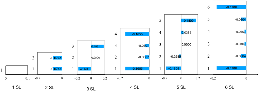
Figure S1: Full numerical results of the SL-resolved effective SOT fields (in the $x$ direction) plotted in the unit of $eEa_{0}/4\pi^{2}\hbar\gamma S$ from 1-SL to 6-SL $\rm MnBi_{2}Te_{4}$. The 1SL case always has a vanishing $H^{\rm T}_{x}$ as guaranteed by symmetry. Parameters: $\gamma_{\rm ex}=75$ meV, $a_{z}=1$ nm.

Using Eq. (3a) in the main text, we can numerically compute the effective field of SOT (driven by an in-plane $\bm{E}$ field) acting on each SL in a 2D $\rm MnBi_{2}Te_{4}$. Since we have adopted a continuum Hamiltonian, we need to first ensure the convergence of our results. To this end, we find that a $100\times 100$ mesh grid in the momentum space truncated at $k_{c}\sim 3$ $\rm nm^{-1}$ already yields good convergence and a well-quantized Chern number. Therefore, to achieve high precision, we adopt a $400\times 400$ mesh grid with momentum truncation $k_{c}=5$ $\rm nm^{-1}$ to compute the SL-specific SOT field from 1-SL to 6-SL samples. The result is shown in Fig. S1. In Fig. 1 of the main text, only the largest component in each case (i.e., $H^{\rm T}_{1,x}$ is shown.

To confirm that the SOT field acting on the inner SLs are always much smaller than $H^{\rm T}_{1,x}$ acting on the outermost SLs, we also plot the relevant components of the SOT field for the 5-SL and 6-SL cases in Fig. S2, where it clearly shows that all $H^{\rm T}_{j,x}$ vary with $\gamma_{ex}$ in a similar pattern and their relative ratios are essentially unchanged. That is to say, $H^{\rm T}_{1,x}$ is always the largest and a representative component, which is why we have only shown $H^{\rm T}_{1,x}$ in the main text.

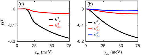
Figure S2: $H^{\rm T}_{x}$ (in unit $eEa_{0}/4\pi^{2}\hbar\gamma S$) for (a) 5-SL and (b) 6-SL $\rm MnBi_{2}Te_{4}$ as functions of the exchange coupling $\gamma_{\rm ex}$.

IV IV. Magnetic resonances for 2-SL and 3-SL $\rm{MnBi_{2}Te_{4}}$

We investigate 2-SL and 3-SL $\rm MnBi_{2}Te_{4}$ as the least non-trivial examples to demonstrate the even-odd contrast in the SOT. To this end, we need to first determine the resonance frequencies and modes as an eigenvalue problem. For the 3-SL case, in the absence of SOT and other external stimuli, the coupled LLG equations are:

$$\dot{\bm{m}}^{1} =\omega_{E}\bm{m}^{1}\times\bm{m}^{2}-(\omega_{0}+\omega_{A}m^{1}_{z})\bm{m}^{1}\times\bm{\hat{z}},$$ (S.13a)

$$\dot{\bm{m}}^{2} =\omega_{E}\bm{m}^{2}\times(\bm{m}^{1}+\bm{m}^{3})-(\omega_{0}+\omega_{A}m^{2}_{z})\bm{m}^{2}\times\bm{\hat{z}},$$ (S.13b)

$$\dot{\bm{m}}^{3} =\omega_{E}\bm{m}^{3}\times\bm{m}^{2}-(\omega_{0}+\omega_{A}m^{3}_{z})\bm{m}^{3}\times\bm{\hat{z}},$$ (S.13c)

where $\omega_{E}=J_{E}/\hbar$, $\omega_{A}=K/\hbar$ and $\omega_{0}=\gamma H_{0}$ are the angular frequencies for the exchange interaction, magnetic anisotropy and external magnetic field (applied in the $\hat{z}$ direction), respectively. We then use the phase vectors $\tilde{m}_{\perp}^{j}=(\tilde{m}^{j}_{x},\tilde{m}^{j}_{y})e^{\mathrm{i}\omega t}$ to linearize the LLG equations around the AFM ground state $\bm{m}^{1(3)}=-\bm{m}^{2}=\hat{\bm{z}}$, arriving at

$$\mathrm{i}\omega\tilde{m}^{1}_{x} =-\omega_{E}(\tilde{m}^{1}_{y}+\tilde{m}^{2}_{y})-(\omega_{0}+\omega_{A})\tilde{m}^{1}_{y},$$ (S.14a)

$$\mathrm{i}\omega\tilde{m}^{1}_{y} =\omega_{E}(\tilde{m}^{2}_{x}+\tilde{m}^{1}_{x})+(\omega_{0}+\omega_{A})\tilde{m}^{1}_{x},$$ (S.14b)

$$\mathrm{i}\omega\tilde{m}^{2}_{x} =\omega_{E}(2\tilde{m}^{2}_{y}+\tilde{m}^{1}_{y}+\tilde{m}^{3}_{y})-(\omega_{0}-\omega_{A})\tilde{m}^{2}_{y},$$ (S.14c)

$$\mathrm{i}\omega\tilde{m}^{2}_{y} =-\omega_{E}(2\tilde{m}^{2}_{x}+\tilde{m}^{1}_{x}+\tilde{m}^{3}_{x})+(\omega_{0}-\omega_{A})\tilde{m}^{2}_{x},$$ (S.14d)

$$\mathrm{i}\omega\tilde{m}^{3}_{x} =-\omega_{E}(\tilde{m}^{3}_{y}+\tilde{m}^{2}_{y})-(\omega_{0}+\omega_{A})\tilde{m}^{3}_{y},$$ (S.14e)

$$\mathrm{i}\omega\tilde{m}^{3}_{y} =\omega_{E}(\tilde{m}^{2}_{x}+\tilde{m}^{3}_{x})+(\omega_{0}+\omega_{A})\tilde{m}^{3}_{x}.$$ (S.14f)

These linearized LLG equations can be formally recast into $\bm{S}\cdot\tilde{\bm{m}}^{T}=\mathrm{i}\omega\tilde{\bm{m}}^{T}$, where $\tilde{\bm{m}}=\tilde{\bm{m}}\equiv[\tilde{m}^{1}_{x},\tilde{m}^{1}_{y},\tilde{m}^{2}_{x},\tilde{m}^{2}_{y},\tilde{m}^{3}_{x},\tilde{m}^{3}_{y}]^{T}$ is a column vector and $\bm{S}$ is the coefficient matrix given by

$$\bm{S}=\begin{bmatrix}0&-(\omega_{0}+\omega_{E}+\omega_{A})&0&-\omega_{E}&0&0\\ (\omega_{0}+\omega_{E}+\omega_{A})&0&\omega_{E}&0&0&0\\ 0&\omega_{E}&0&(-\omega_{0}+2\omega_{E}+\omega_{A})&0&\omega_{E}\\ -\omega_{E}&0&(\omega_{0}-2\omega_{E}-\omega_{A})&0&-\omega_{E}&0\\ 0&0&0&-\omega_{E}&0&-(\omega_{0}+\omega_{E}+\omega_{A})\\ 0&0&\omega_{E}&0&(\omega_{0}+\omega_{E}+\omega_{A})&0\end{bmatrix},$$ (S.15)

whose eigenvalues $\lambda$ give the resonance frequencies by $\omega=-\mathrm{i}\lambda$, reproducing Eq. (5) in the main text. The three eigenfrequencies are plotted in Fig. S3(a) as functions of the applied magnetic field. The corresponding eigenmodes (given by the eigenvectors of the $\bm{S}$ matrix) are illustrated in Fig. (3d) in the main text.

We next add the SOT field $\bm{H}_{j}^{\rm T}$ for each $\bm{m}^{j}$ (an AC field generated by $Ee^{\mathrm{i}\omega t}$) and the Gilbert damping in the LLG equations:

$$\dot{\bm{m}}^{1} =\omega_{E}\bm{m}^{1}\times\bm{m}^{2}-\gamma\bm{m}^{1}\times\bm{H}^{\rm T}_{1}-(\omega_{0}+\omega_{A})\bm{m}^{1}\times\bm{\hat{z}}+\alpha_{G}\bm{m}^{1}\times\dot{\bm{m}}^{1},$$ (S.16a)

$$\dot{\bm{m}}^{2} =\omega_{E}\bm{m}^{2}\times(\bm{m}^{1}+\bm{m}^{3})-\gamma\bm{m}^{2}\times\bm{H}^{\rm T}_{2}-(\omega_{0}-\omega_{A})\bm{m}^{2}\times\bm{\hat{z}}+\alpha_{G}\bm{m}^{2}\times\dot{\bm{m}}^{2},$$ (S.16b)

$$\dot{\bm{m}}^{3} =\omega_{E}\bm{m}^{3}\times\bm{m}^{2}-\gamma\bm{m}^{3}\times\bm{H}^{\rm T}_{3}-(\omega_{0}+\omega_{A})\bm{m}^{3}\times\bm{\hat{z}}+\alpha_{G}\bm{m}^{3}\times\dot{\bm{m}}^{3},$$ (S.16c)

where $\bm{H}^{\rm T}_{1}=-\bm{H}^{\rm T}_{3}$ and $\bm{H}^{\rm T}_{2}=0$. Using the phasor notations followed by a similar procedure as above to linearize the LLG equations, we find that $\tilde{m}^{2}_{x}=\tilde{m}^{2}_{y}=0$, $\tilde{m}^{1}_{x}=-\tilde{m}^{3}_{x}=\tilde{\chi}_{\parallel}\tilde{H}^{\rm T}_{1,x}$ and $\tilde{m}^{1}_{y}=-\tilde{m}^{3}_{y}=\tilde{\chi}_{\perp}\tilde{H}^{\rm T}_{1,x}$ where the longitudinal and transverse components of the magnetic susceptibility are

$$\tilde{\chi}_{\parallel}(\omega)=\frac{-(\mathrm{i}\alpha_{G}\omega+\omega_{3}^{r})}{\omega^{2}-(\mathrm{i}\alpha_{G}\omega+\omega_{3}^{r})^{2}},$$ (S.17a)

$$\tilde{\chi}_{\perp}(\omega)=\frac{\mathrm{i}\omega}{\omega^{2}-(\mathrm{i}\alpha_{G}\omega+\omega_{3}^{r})^{2}},$$ (S.17b)

with $\omega_{3}^{r}=\omega_{0}+\omega_{A}+\omega_{E}$ corresponding to the green line in Fig. S3(a). Equations (S.17a) and (S.17b) reproduce Eqs. (6a) and (6b) in the main text.

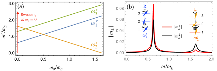
Figure S3: (a) Magnetic resonance frequencies as a function of $\omega_{0}$ in a 3-SL $\rm MnBi_{2}Te_{4}$. The read arrow marks the frequency sweep at zero bias field. (b) The amplitude of magnetization precession of $\bm{m}^{1}$ (red) and $\bm{m}^{2}$ (black) as a function of the driving frequency. Parameters: $\hbar\omega_{E}=0.272\ \rm meV$, $\hbar\omega_{A}=0.084\ \rm meV$, $H_{x}^{\rm micro}=H_{y}^{\rm micro}=36\ \rm Oe$.

While the $\omega_{3}^{r}$ mode can be exclusively excited by the SOT as discussed in the main text, the AFM resonance modes $\omega_{1}^{r}$ and $\omega_{2}^{r}$, on the other hand, can be excited by a microwave with SL-independent magnetic field $\tilde{\bm{H}}^{\rm T}_{1}=\tilde{\bm{H}}^{\rm T}_{2}=\tilde{\bm{H}}^{\rm T}_{3}=(H_{x}^{\rm micro},H_{y}^{\rm micro})e^{\mathrm{i}\omega t}$. In the absence of bias field [$\omega_{0}=0$, see the red arrow in Fig. S3(a)], we numerically calculate the amplitude of the dynamical components of $\bm{m}^{j}$ as functions of the driving frequency. The result is plotted in Fig. S3(b), where we see resonance peaks at both $\omega_{1}^{r}$ and $\omega_{2}^{r}$ but not $\omega_{3}^{r}$, which is exactly opposite to the SOT-driven resonance. We notice that in the $\omega^{r}_{1}$ ($\omega^{r}_{2}$) mode, the in-plane magnetization satisfies $|\bm{m}^{1}_{\perp}/|\bm{m}^{2}_{\perp}|>1$ ($|\bm{m}^{1}_{\perp}/|\bm{m}^{2}_{\perp}|<1$); the exact ratio depends on $\omega_{A}/\omega_{E}$

Similarly, we can analyze the SOT-induced AFM resonances in a 2-SL $\rm MnBi_{2}Te_{4}$. Linearizing the coupled LLG equations for $\bm{m}^{1}$ and $\bm{m}^{2}$ gives

$$\mathrm{i}\omega\tilde{m}^{1}_{x} =-\omega_{E}(\tilde{m}^{1}_{y}+\tilde{m}^{2}_{y})-(\omega_{0}+\omega_{A})\tilde{m}^{1}_{y},$$ (S.18a)

$$\mathrm{i}\omega\tilde{m}^{1}_{y} =\omega_{E}(\tilde{m}^{2}_{x}+\tilde{m}^{1}_{x})+(\omega_{0}+\omega_{A})\tilde{m}^{1}_{x},$$ (S.18b)

$$\mathrm{i}\omega\tilde{m}^{2}_{x} =\omega_{E}(\tilde{m}^{2}_{y}+\tilde{m}^{1}_{y})-(\omega_{0}-\omega_{A})\tilde{m}^{2}_{y},$$ (S.18c)

$$\mathrm{i}\omega\tilde{m}^{2}_{y} =-\omega_{E}(\tilde{m}^{2}_{x}+\tilde{m}^{1}_{x})+(\omega_{0}-\omega_{A})\tilde{m}^{2}_{x},$$ (S.18d)

from which one can easily obtain the eigenfrequencies $\omega^{r}_{1(2)}=\sqrt{\omega_{A}(2\omega_{E}+\omega_{A})}\pm\omega_{0}$. The corresponding eigenmodes are the familiar right-handed and left-handed chiral modes depicted in Fig. (3b) of the main text. After adding the voltage-induced SOT field $\bm{H}^{\rm T}_{1}=\bm{H}^{\rm T}_{2}$, which in the 2-SL case acts similarly as a microwave, the coupled LLG equations become

$$\dot{\bm{m}}^{1} =\omega_{E}\bm{m}^{1}\times\bm{m}^{2}-\bm{m}^{1}\times\bm{H}^{T}_{1}-(\omega_{0}+\omega_{A})\bm{m}^{1}\times\bm{\hat{z}}+\alpha_{G}\bm{m}^{1}\times\dot{\bm{m}}^{1},$$ (S.19a)

$$\dot{\bm{m}}^{2} =\omega_{E}\bm{m}^{2}\times\bm{m}^{1}-\bm{m}^{2}\times\bm{H}^{T}_{2}-(\omega_{0}-\omega_{A})\bm{m}^{2}\times\bm{\hat{z}}+\alpha_{G}\bm{m}^{2}\times\dot{\bm{m}}^{2}.$$ (S.19b)

For $\omega_{0}=0$ (no bias field), linearizing Eq. (S.19) in terms of $\tilde{m}^{j}_{\perp}$ yields $\tilde{m}^{1}_{x}=\tilde{m}^{2}_{x}=\tilde{\chi}_{\parallel}\tilde{H}^{\rm T}_{1,x}$ and $\tilde{m}^{1}_{y}=-\tilde{m}^{2}_{y}=\tilde{\chi}_{\perp}\tilde{H}^{\rm T}_{1,x}$, which describes a linearly-polarized oscillation of the Néel vector $\bm{n}=(\bm{m}^{1}-\bm{m}^{2})/2$ in the $y-z$ plane (the total magnetization $\bm{m}=\bm{m}^{1}+\bm{m}^{2}$, on the other hand, oscillates in the $x-z$ plane). This is because the two resonance modes are degenerate ($\omega_{1}^{r}=\omega_{2}^{r}$) for $\omega_{0}=0$ so that a linearly-polarized electric field (hence a linearly-polarized SOT field) simultaneously drive the two modes with the same amplitude, forming a pure linearly-polarized response. In this case, the magnetic susceptibility

$$\tilde{\chi}_{\parallel}(\omega)=\frac{-(\mathrm{i}\alpha_{G}\omega+\omega_{A})}{\omega^{2}-(\mathrm{i}\alpha_{G}\omega+\omega_{A})^{2}-2\omega_{E}(\mathrm{i}\alpha_{G}\omega+\omega_{A})}$$ (S.20a)

$$\tilde{\chi}_{\perp}(\omega)=\frac{\mathrm{i}\omega}{\omega^{2}-(\mathrm{i}\alpha_{G}\omega+\omega_{A})^{2}-2\omega_{E}(\mathrm{i}\alpha_{G}\omega+\omega_{A})}$$ (S.20b)

exhibits a single maximum in amplitude at around $\omega_{1}^{r}=\omega_{2}^{r}=\sqrt{\omega_{A}(2\omega_{E}+\omega_{A})}$ (the actual maximum point should be slightly red-shifted from the exact value due to $\alpha_{G}$). To selectively excite the two chiral modes without mixing, we will in the following include a finite bias field $\omega_{0}$ (not strong enough to trigger the spin-flop transition) to lift the degeneracy of the two modes when discussing the 2-SL AFM resonance.

While the driving electric field $Ee^{\mathrm{i}\omega t}$ generates the SOT field through the spin-orbit coupling and the exchange coupling between electrons and magnetic moments, it also generates an Oersted field according to the Maxwell equations. Moreover, for an even-SL $\rm MnBi_{2}Te_{4}$, the topological axion field ($\theta=\pi$ inside and $0$ outside the material) brings about topological magnetoelectric (TME) responses. These two effects are reflected in the modified Ampère’s law

$$\nabla\times\bm{B}=\mu_{0}\epsilon_{0}\epsilon_{r}\frac{\partial\bm{E}}{\partial t}+\frac{\alpha}{c\pi}\bm{\nabla}\theta\times\bm{E},$$ (S.21)

where $\varepsilon_{0}$ and $\mu_{0}$ are the vacuum permittivity and permeability, $\varepsilon_{r}\approx 1$ is the relative permittivity, $\alpha=1/137$ is the fine structure constant, and $c$ is the speed of light. In a few-SL system, the thickness $d$ is much smaller than the width $w$, so the Oersted field generated by the displacement current $\mu_{0}\epsilon_{0}\epsilon_{r}\partial\bm{E}/\partial t$ is approximately $\bm{B}(t)\approx-\hat{\bm{y}}\mu_{0}\epsilon_{0}\epsilon_{r}\omega E_{x}(t)d/2$, which is perpendicular to $\bm{E}$. As an estimation, an electric field drive of strength $E_{x}=1{\rm V/\mu m}$ and frequency $\omega/2\pi=100{\rm GHz}$ generates an Oersted field of only $B\sim 1\times 10^{-7}$T for $d\sim$ a few nm. The TME effect generates a magnetic field through the second term on the right hand side of Eq. (S.21), which is roughly collinear with $\bm{E}$ and is estimated by $B^{\rm TME}=\mu_{0}\sigma_{H}E$ with $\sigma_{H}$ the half-quantized Hall conductance on the outermost SL. Then $B^{\rm TME}\sim 10^{-5}\rm\ T$ for $E_{x}=1\ {\rm V/\mu m}$. As a comparison, the SOT field generated by the same electric field is on the order of $10^{-3}{\rm\ T}$ to $10^{-2}{\rm\ T}$, which is much larger than both the Oersted field and $B^{\rm TME}$. This indicates the dominant role of the SOT effect in 2D magnets as compared to other field-induced effects, as illustrated in Fig. S4. In stark contrast, the Oersted field and the SOT field in a current-driven 3D heterostructure [10] have comparable strengths.

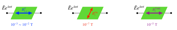
Figure S4: From left to right: SOT field, Oersted field, and TME field generated by an in-plane ac electric field of strength $|\tilde{E}|=1\rm\ V/\mu m$.

V V. Topological charge pumping

When the SL-dependent magnetic moments are driven into motion, they pump an in-plane current density $\bm{J}^{\rm P}=\{J^{\rm p}_{x},J^{\rm p}_{y}\}$ that

$$J^{\rm p}_{x}(t)=-e\dot{m}_{x}^{j}\cdot\langle{\rm Tr}(\Omega^{m^{j}k}_{xx})\rangle-e\dot{m}_{y}^{j}\cdot\langle{\rm Tr}(\Omega^{m^{j}k}_{yx})\rangle,$$ (S.22)

$$J^{\rm p}_{y}(t)=-e\dot{m}_{x}^{j}\cdot\langle{\rm Tr}(\Omega^{m^{j}k}_{xy})\rangle-e\dot{m}_{y}^{j}\cdot\langle{\rm Tr}(\Omega^{m^{j}k}_{yy})\rangle,$$ (S.23)

where $\langle(\cdots)\rangle=1/(2\pi)^{2}\int{\rm d}^{2}kf(\bm{k})(\cdots)$ denotes the average over the first Brillouin zone. Through numerical calculation, we find that $\Omega_{xy}^{m^{j}k}$ and $\Omega_{yx}^{m^{j}k}$ vanish, which is consistent with the vanishing SOT fields perpendicular to the applied $\bm{E}$ field. In phasor notations, Eqs. (S.22) and  (S.23), the $\omega_{3}^{r}$ mode of a 3-SL $\rm MnBi_{2}Te_{4}$ pumps

$$\tilde{J}^{\rm p}_{x}=-e\dot{\tilde{m}}_{x}^{1}\cdot\langle{\rm Tr}(\Omega^{m^{1}k}_{xx})\rangle-e\dot{\tilde{m}}_{x}^{3}\cdot\langle{\rm Tr}(\Omega^{m^{3}k}_{xx})\rangle,$$ (S.24)

$$\tilde{J}^{\rm p}_{y}=-e\dot{\tilde{m}}_{y}^{1}\cdot\langle{\rm Tr}(\Omega^{m^{1}k}_{yy})\rangle-e\dot{\tilde{m}}_{y}^{3}\cdot\langle{\rm Tr}(\Omega^{m^{3}k}_{yy})\rangle.$$ (S.25)

where the middle SL does not contribute because $\bm{m}^{2}$ stays static (also, $\langle\Omega^{m^{2}k}_{\mu\nu}\rangle=0$). Using $\tilde{H}_{j,x}^{\rm T}=ea_{0}^{2}\langle{\rm Tr}(\Omega^{km^{j}}_{xx})\rangle\tilde{E}_{x}/\gamma\hbar S$, and the relations $\tilde{m}^{1}_{x(y)}=\tilde{\chi}_{\parallel(\perp)}\gamma\tilde{H}^{\rm T}_{1,x}$, $\tilde{m}^{3}_{x(y)}=\tilde{\chi}_{\parallel(\perp)}\gamma\tilde{H}^{\rm T}_{3,x}$ and $\tilde{H}^{\rm T}_{1,x}=-\tilde{H}^{\rm T}_{3,x}$, we can rewrite Eq. (S.24) and  (S.25) as

$$\tilde{J}^{\rm p}_{x}= \mathrm{i}\omega\tilde{E}_{x}\tilde{\chi}_{\parallel}\frac{e^{2}a_{0}^{2}}{\hbar S}\langle{\rm Tr}(\Omega^{km^{1}}_{xx})\rangle\left[\langle{\rm Tr}(\Omega^{km^{1}}_{xx})\rangle-\langle{\rm Tr}(\Omega^{km^{3}}_{xx})\rangle\right],$$ (S.26)

$$\tilde{J}^{\rm p}_{y}= \mathrm{i}\omega\tilde{E}_{x}\tilde{\chi}_{\perp}\frac{e^{2}a_{0}^{2}}{\hbar S}\langle{\rm Tr}(\Omega^{km^{1}}_{xx})\rangle\left[\langle{\rm Tr}(\Omega^{km^{1}}_{yy})\rangle-\langle{\rm Tr}(\Omega^{km^{3}}_{yy})\rangle\right],$$ (S.27)

where we have use the antisymmetric property of the Berry curvature $\Omega^{km}_{\mu\nu}=-\Omega^{mk}_{\mu\nu}$. By symmetry, $\Omega^{km^{1}}_{xx}=\Omega_{yy}^{km^{1}}=-\Omega^{km^{3}}_{xx}=-\Omega^{km^{3}}_{yy}$, so we can read off the effective conductivity from $\bm{J}^{\rm P}$ as

$$\tilde{\sigma}_{xx} =\frac{\tilde{J}^{\rm p}_{x}}{\tilde{E}_{x}}=\mathrm{i}\omega\tilde{\chi}_{\parallel}(\omega)\frac{2e^{2}a_{0}^{2}}{\hbar S}\left\langle{\rm Tr}(\Omega_{xx}^{km^{1}})\right\rangle^{2},$$ (S.28a)

$$\tilde{\sigma}_{yx} =\frac{\tilde{J}^{\rm p}_{y}}{\tilde{E}_{x}}=\mathrm{i}\omega\tilde{\chi}_{\perp}(\omega)\frac{2e^{2}a_{0}^{2}}{\hbar S}\left\langle{\rm Tr}(\Omega_{yy}^{km^{1}})\right\rangle^{2},$$ (S.28b)

which reproduces Eqs. (7a) and (7b) in the main text.

Following a similar procedure, we can also obtain the effective conductivity for a 2-SL $\rm MnBi_{2}Te_{4}$. However, it should be noted that in the chiral AFM resonance modes, $\bm{m}^{1}$ and $\bm{m}^{2}$ precess with different cone angles (i.e. different amplitudes). Therefore, we cannot use a single dynamical susceptibility $\tilde{\chi}_{\parallel(\perp)}$ as that in the 3-SL case, but instead we need to define the SL-specific susceptibility as $\tilde{\chi}_{\parallel(\perp)}^{j}=\tilde{m}^{j}_{x(y)}/\gamma\tilde{H}_{x}^{\rm T}$ ($j=1,2$) where $\tilde{H}_{x}^{\rm T}$ is the same for both SLs. After some algebra, we have

$$\tilde{\sigma}_{xx} =\mathrm{i}\omega\frac{e^{2}a_{0}^{2}}{\hbar S}\left\langle{\rm Tr}(\Omega_{xx}^{km^{1}})\right\rangle\left[\langle{\rm Tr}(\Omega^{km^{1}}_{xx})\rangle\tilde{\chi}^{1}_{\parallel}+\langle{\rm Tr}(\Omega^{km^{2}}_{xx})\rangle\tilde{\chi}^{2}_{\parallel}\right],$$ (S.29a)

$$\tilde{\sigma}_{yx} =\mathrm{i}\omega\frac{e^{2}a_{0}^{2}}{\hbar S}\left\langle{\rm Tr}(\Omega_{xx}^{km^{1}})\right\rangle\left[\langle{\rm Tr}(\Omega^{km^{1}}_{yy})\rangle\tilde{\chi}^{1}_{\perp}+\langle{\rm Tr}(\Omega^{km^{2}}_{yy})\rangle\tilde{\chi}^{2}_{\perp}\right],$$ (S.29b)

where the Berry curvature satisfies $\Omega^{km^{1}}_{xx}=\Omega_{yy}^{km^{1}}=\Omega^{km^{2}}_{xx}=\Omega^{km^{2}}_{yy}$. If $\bm{m}^{1}$ and $\bm{m}^{2}$ precess with the same amplitude (and out of phase), we would have $\tilde{\chi}^{1}_{\perp(\parallel)}=-\tilde{\chi}^{2}_{\perp(\parallel)}$ and thus an identically vanishing conductivity. It is because the two SLs have different amplitudes, hence $\tilde{\chi}^{1}_{\perp(\parallel)}\neq-\tilde{\chi}^{2}_{\perp(\parallel)}$, that the two terms in the bracket do not cancel and the conductivity becomes non-zero. This explains why the peak values of the 2-SL AFM resonances are much smaller than that of the $\omega_{3}^{r}$ resonance in the 3-SL case (see Fig. 4 in the main text). In other words, the SLs constructively (destructively) contribute to the topological charge pumping in the 3-SL (2-SL) electric field-driven magnetic resonance.

VI VI. Mechanical efficiency and effective circuit

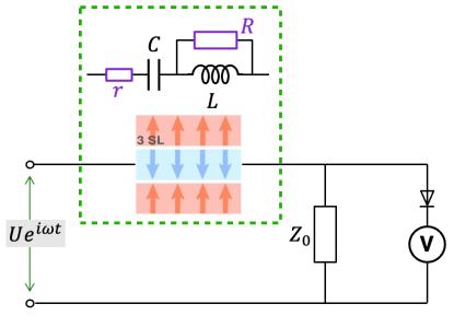
Figure S5: Effective circuit of a 3-SL $\rm MnBi_{2}Te_{4}$ (enclosed in the dashed green rectangle) and the detection circuit of the $\omega_{3}^{r}$ resonance.

The total electric power is $P_{J}=\overline{J^{\rm p}_{x}E_{x}}l_{x}l_{y}$ where the time average reads $\overline{J_{x}E_{x}}=\int_{0}^{T}J_{x}E_{x}dt/T$ with $T=2\pi/\omega$. From circuit theory, it can be straightforwardly derived that [39]

$$P_{J}=\frac{1}{2}E_{x}^{2}l_{x}l_{y}{\rm Re}[\sigma_{xx}]=E_{x}^{2}l_{x}l_{y}\frac{e^{2}a_{0}^{2}}{\hbar S}\left\langle{\rm Tr}(\Omega^{km^{1}}_{xx})\right\rangle^{2}\omega{\rm Im}(\tilde{\chi}_{\parallel}),$$ (S.30)

where Eq. (S.28a) is used. The time-averaged magnetic dissipation power (for the 3-SL case) is

$$P_{M}=\alpha_{\rm G}\hbar Sl_{x}l_{y}\left(\overline{|\dot{\bm{m}}^{1}|^{2}}+\overline{|\dot{\bm{m}}^{3}|^{2}}\right)/a_{0}^{2}=2\alpha_{\rm G}\hbar Sl_{x}l_{y}\overline{|\dot{\bm{m}}^{1}|^{2}}/a_{0}^{2},$$ (S.31)

where $|\dot{\bm{m}}^{1}(t)|^{2}=[\dot{m}^{1}_{x}(t)]^{2}+[\dot{m}^{1}_{y}(t)]^{2}$. In phasor notations, after time average we have $P_{M}=\alpha_{G}\hbar Sl_{x}l_{y}\omega^{2}(|\tilde{m}^{1}_{x}|^{2}+|\tilde{m}^{1}_{y}|^{2})/a_{0}^{2}$. Since $\tilde{m}^{1}_{x(y)}=\tilde{\chi}^{1}_{\parallel(\perp)}\gamma\tilde{H}^{\rm T}_{1,x}$ and $\tilde{H}_{1,x}^{\rm T}=ea_{0}^{2}\langle{\rm Tr}(\Omega^{km^{1}}_{xx})\rangle\tilde{E}_{x}/\gamma\hbar S$, we have $|\tilde{m}^{1}_{x(y)}|=(ea_{0}^{2}E_{x}/\hbar S)|\tilde{\chi}^{1}_{\parallel(\perp)}|\left\langle{\rm Tr}(\Omega^{km^{1}}_{xx})\right\rangle$. Then $P_{M}$ becomes

$$P_{M}=\alpha_{G}E_{x}^{2}l_{x}l_{y}\frac{e^{2}a_{0}^{2}}{\hbar S}\left\langle{\rm Tr}(\Omega^{km^{1}}_{xx})\right\rangle^{2}\omega^{2}(|\tilde{\chi}_{\parallel}|^{2}+|\tilde{\chi}_{\perp}|^{2}).$$ (S.32)

Combing Eq. (S.30) and Eq. (S.32), we obtain the mechanical efficiency

$$\xi=\frac{P_{M}}{P_{J}}=\frac{\alpha_{G}\omega(|\tilde{\chi}_{\parallel}|^{2}+|\tilde{\chi}_{\perp}|^{2})}{{\rm Im}(\tilde{\chi}_{\parallel})}.$$ (S.33)

From Eqs. (S.17a) and (S.17b), we also have the following expressions:

$$|\tilde{\chi}_{\parallel}|^{2}=\frac{\alpha_{G}^{2}\omega^{2}+(\omega_{3}^{r})^{2}}{(1+\alpha_{G}^{2})^{2}\omega^{4}+2(\alpha_{G}^{2}-1)\omega^{2}(\omega_{3}^{r})^{2}+(\omega_{3}^{r})^{4}},$$ (S.34)

$$|\tilde{\chi}_{\perp}|^{2}=\frac{\omega^{2}}{(1+\alpha_{G}^{2})^{2}\omega^{4}+2(\alpha_{G}^{2}-1)\omega^{2}(\omega_{3}^{r})^{2}+(\omega_{3}^{r})^{4}},$$ (S.35)

$${\rm Im}[\tilde{\chi}_{\parallel}]=\frac{-\alpha_{G}\omega[(1+\alpha_{G}^{2})\omega^{2}+(\omega_{3}^{r})^{2}]}{(1+\alpha_{G}^{2})^{2}\omega^{4}+2(\alpha_{G}^{2}-1)\omega^{2}(\omega_{3}^{r})^{2}+(\omega_{3}^{r})^{4}}.$$ (S.36)

Inserting the above relations into Eq. (S.33) yields $\xi=1$, which justifies Eq. (8) of the main text.

The longitudinal electrical response of a 3-SL $\rm MnBi_{2}Te_{4}$ can be mapped to an effective $RLC$ circuit following the idea of Ref. [39]. From Eq. (S.28a) and Eq. (S.17a), the effective longitudinal impedance of the device becomes

$$Z_{\rm sys}=\frac{l_{x}}{l_{y}\tilde{\sigma}_{xx}}=Z_{m}\left[\frac{-(1+\alpha^{2})\omega^{2}+(\omega^{r}_{3})^{2}+2i\alpha\omega\omega^{r}_{3}}{i\omega\omega^{r}_{3}-\alpha\omega^{2}}\right]=Z_{m}\left(\alpha+\frac{\omega^{r}_{3}}{i\omega}\right)+\frac{Z_{m}}{\left(\alpha+\frac{\omega^{r}_{3}}{i\omega}\right)},$$ (S.37)

where $Z_{m}=\hbar Sl_{x}/(2l_{y}e^{2}a_{0}^{2}\langle{\rm Tr}(\Omega^{km^{1}}_{xx})\rangle^{2})$. The form of the impedance is equivalent to that of a $RLC$ circuit drawn in Fig. S5, whose impedance is $Z_{\rm eff}=r+1/i\omega C+i\omega LR/(i\omega L+R)$. By setting $Z_{\rm sys}=Z_{\rm eff}$, we obtain

$$R=\frac{Z_{m}}{\alpha_{G}},\ \ r=Z_{m}\alpha_{G},\ \ L=\frac{Z_{m}}{\omega^{r}_{3}},\ \ C=\frac{1}{Z_{m}\omega^{r}_{3}},$$ (S.38)

where we emphasize that $R$ and $r$ represent the magnetic Gilbert damping but has nothing to do with Ohm’s conduction.

Fig. S5 also illustrates the schematics of detecting the $\omega_{3}^{r}$ resonance. When $\omega$ approaches $\omega^{r}_{3}$, the longitudinal conductivity $\tilde{\sigma}_{xx}$ approaches the maximum [see Fig.4(a) in the main text] so $Z_{\rm sys}$ approaches the minimum. Then, the voltage drop (as read off from the voltmeter) on the reference impedance $Z_{0}$ will experience a resonance peak. When the system goes off-resonance, the conductivity will rapidly drop to zero, so will the voltage drop on $Z_{0}$.

References

Shao et al. [2021]Q. Shao, P. Li, L. Liu, H. Yang, S. Fukami, A. Razavi, H. Wu, K. Wang, F. Freimuth,
Y. Mokrousov, M. D. Stiles, S. Emori, A. Hoffmann, J. Åkerman, K. Roy, J.-P. Wang, S.-H. Yang, K. Garello, and W. Zhang, Roadmap of spin–orbit torques, IEEE Transactions on Magnetics 57, 1 (2021).
Manchon et al. [2019]A. Manchon, J. Železný, I. M. Miron, T. Jungwirth, J. Sinova, A. Thiaville, K. Garello, and P. Gambardella, Current-induced spin-orbit torques in ferromagnetic and antiferromagnetic
systems, Rev. Mod. Phys. 91, 035004 (2019).
Hoffmann and Bader [2015]A. Hoffmann and S. D. Bader, Opportunities at the
frontiers of spintronics, Phys. Rev. Appl. 4, 047001 (2015).
Žutić et al. [2004]I. Žutić,
J. Fabian, and S. Das Sarma, Spintronics: Fundamentals and applications, Rev. Mod. Phys. 76, 323 (2004).
Zhu et al. [2019]L. Zhu, D. C. Ralph, and R. A. Buhrman, Spin-orbit torques in
heavy-metal–ferromagnet bilayers with varying strengths of interfacial
spin-orbit coupling, Phys. Rev. Lett. 122, 077201 (2019).
Han et al. [2017]J. Han, A. Richardella,
S. A. Siddiqui, J. Finley, N. Samarth, and L. Liu, Room-temperature spin-orbit torque switching induced by a
topological insulator, Phys. Rev. Lett. 119, 077702 (2017).
Mellnik et al. [2014]A. R. Mellnik, J. S. Lee,
A. Richardella, J. L. Grab, P. J. Mintun, M. H. Fischer, A. Vaezi, A. Manchon, E.-A. Kim, N. Samarth, and D. C. Ralph, Spin-transfer torque
generated by a topological insulator, Nature 511, 449 (2014).
Fan et al. [2014]Y. Fan, P. Upadhyaya,
X. Kou, M. Lang, S. Takei, Z. Wang, J. Tang, L. He, L.-T. Chang, M. Montazeri, G. Yu, W. Jiang, T. Nie, R. N. Schwartz, Y. Tserkovnyak, and K. L. Wang, Magnetization switching
through giant spin–orbit torque in a magnetically doped topological
insulator heterostructure, Nature Materials 13, 699 (2014).
Liu et al. [2012]L. Liu, C.-F. Pai,
Y. Li, H. W. Tseng, D. C. Ralph, and R. A. Buhrman, Spin-torque switching with the giant spin hall effect of
tantalum, Science 336, 555 (2012).
Liu et al. [2011]L. Liu, T. Moriyama,
D. C. Ralph, and R. A. Buhrman, Spin-torque ferromagnetic resonance
induced by the spin hall effect, Phys. Rev. Lett. 106, 036601 (2011).
Miron et al. [2011]I. M. Miron, K. Garello,
G. Gaudin, P.-J. Zermatten, M. V. Costache, S. Auffret, S. Bandiera, B. Rodmacq, A. Schuhl, and P. Gambardella, Perpendicular switching of a single ferromagnetic layer induced by in-plane
current injection, Nature 476, 189 (2011).
Mihai Miron et al. [2010]I. Mihai Miron, G. Gaudin,
S. Auffret, B. Rodmacq, A. Schuhl, S. Pizzini, J. Vogel, and P. Gambardella, Current-driven spin torque induced by the rashba effect in a ferromagnetic
metal layer, Nature materials 9, 230 (2010).
Johansen et al. [2019]O. Johansen, V. Risinggård, A. Sudbø, J. Linder, and A. Brataas, Current Control of Magnetism in
Two-Dimensional , Phys. Rev. Lett. 122, 217203 (2019).
Kurebayashi et al. [2022]H. Kurebayashi, J. H. Garcia, S. Khan,
J. Sinova, and S. Roche, Magnetism, symmetry and spin transport in van der waals
layered systems, Nature Reviews Physics 4, 150 (2022).
Zhang et al. [2021]K. Zhang, S. Han, Y. Lee, M. J. Coak, J. Kim, I. Hwang, S. Son, J. Shin, M. Lim, D. Jo, et al., Gigantic current control of coercive field and
magnetic memory based on nanometer-thin ferromagnetic van der Waals
, Advanced Materials 33, 2004110 (2021).
Xue and Haney [2021]F. Xue and P. M. Haney, Intrinsic staggered
spin-orbit torque for the electrical control of antiferromagnets: Application
to , Phys. Rev. B 104, 224414 (2021).
Otrokov et al. [2019]Otrokov, Klimovskikh, and et al., Prediction and observation
of an antiferromagnetic topological insulator, Nature 576, 416 (2019).
Chen et al. [2019]B. Chen, F. Fei, D. Zhang, B. Zhang, W. Liu, S. Zhang, P. Wang,
B. Wei, Y. Zhang, Z. Zuo, et al., Intrinsic magnetic topological insulator phases in the Sb doped
bulks and thin flakes, Nature communications 10, 4469 (2019).
Li et al. [2019]J. Li, L. Yang, D. Shiqiao, Z. Wang, G. Bing-Lin, Z. Shou-Cheng, K. He, D. Wenhui, and Y. Xu, Intrinsic magnetic topological
insulators in van der Waals layered
-family materials, Sci. Adv. 5, 10.1126/sciadv.aaw5685 (2019).
Zhang et al. [2019]D. Zhang, M. Shi, T. Zhu, D. Xing, H. Zhang, and J. Wang, Topological Axion States in the Magnetic Insulator
with the Quantized Magnetoelectric
Effect, Phys. Rev. Lett. 122, 206401 (2019).
Gong et al. [2019]Y. Gong, J. Guo, J. Li, K. Zhu, M. Liao, X. Liu, Q. Zhang, L. Gu, L. Tang, X. Feng, D. Zhang, W. Li, C. Song, L. Wang, P. Yu, X. Chen, Y. Wang, H. Yao, W. Duan, Y. Xu, S.-C. Zhang, X. Ma, Q.-K. Xue, and K. He, Experimental realization of an intrinsic magnetic
topological insulator, Chinese Physics Letters 36, 076801 (2019).
Deng et al. [2020]Y. Deng, Y. Yu, M. Shi, Z. Guo, Z. Xu, J. Wang, X. Chen, and Y. Zhang, Quantum anomalous Hall effect in intrinsic
magnetic topological insulator , Science 367, 10.1126/science.aax8156 (2020).
Liu et al. [2020]C. Liu, Y. Wang, H. Li, Y. Wu, Y. Li, J. Li, K. He, Y. Xu, J. Zhang, and Y. Wang, Robust axion insulator and chern insulator phases in a
two-dimensional antiferromagnetic topological insulator, Nature Materials 19, 522 (2020).
Ovchinnikov et al. [2021]D. Ovchinnikov, X. Huang,
Z. Lin, Z. Fei, J. Cai, T. Song, M. He, Q. Jiang, C. Wang, H. Li, et al., Intertwined topological and magnetic orders in atomically thin
Chern insulator , Nano letters 21, 2544 (2021).
Yang et al. [2021]S. Yang, X. Xu, Y. Zhu, R. Niu, C. Xu, Y. Peng, X. Cheng,
X. Jia, Y. Huang, X. Xu, J. Lu, and Y. Ye, Odd-Even Layer-Number Effect and
Layer-Dependent Magnetic Phase Diagrams in
, Phys. Rev. X 11, 011003 (2021).
Zhao et al. [2021]Y.-F. Zhao, L.-J. Zhou,
F. Wang, G. Wang, T. Song, D. Ovchinnikov, H. Yi,
R. Mei, K. Wang, M. H. Chan, et al., Even–odd layer-dependent anomalous Hall effect in topological
magnet thin films, Nano letters 21, 7691 (2021).
Xiao et al. [2010]D. Xiao, M.-C. Chang, and Q. Niu, Berry phase effects on electronic properties, Rev. Mod. Phys. 82, 1959 (2010).
Cheng and Niu [2012]R. Cheng and Q. Niu, Electron dynamics in slowly varying
antiferromagnetic texture, Phys. Rev. B 86, 245118 (2012).
[31]For non-Abelian Berry curvature, is gauge invariant while itself is gauge covariant. The
summation over band index is not shown explicitly, but it has been taken care
of in numerical calculations.
Li and Cheng [2022]Y.-H. Li and R. Cheng, Quantum interference in a
superconductor--superconductor
Josephson junction, Phys. Rev. Res. 4, 033227 (2022).
Keffer and Kittel [1952]F. Keffer and C. Kittel, Theory of
antiferromagnetic resonance, Phys. Rev. 85, 329 (1952).
Tang and Cheng [2022]J.-Y. Tang and R. Cheng, Voltage-driven exchange resonance
achieving 100% mechanical efficiency, Phys. Rev. B 106, 054418 (2022).
[40]The peak values of
and are approximately two orders of magnitude smaller
than the QAH conductivity . Consequently, could be
overwhelmed by the QAH current. Nonetheless, the phase of
is behind on resonance, while the
QAH signal is in phase with , so the two effects can be
distinguished. After all, is unambiguous as it is unique to the
topological charge pumping.
Supplemental Material for “Efficient Spin-Orbit Torques in Antiferromagnetic Topological Insulator MnBi2Te4”
1Department of Physics and Astronomy, University of California, Riverside, California 92521, USA
2Department of Electrical and Computer Engineering, University of California, Riverside, California 92521, USA