Matrix logistic map: fractal spectral distributions and transfer of chaos

Abstract

The standard logistic map, $x^{\prime}=ax(1-x)$, serves as a paradigmatic model to demonstrate how apparently simple non-linear equations lead to complex and chaotic dynamics. In this work we introduce and investigate its matrix analogue defined for an arbitrary matrix $X$ of a given order $N$. We show that for an arbitrary initial ensemble of hermitian random matrices with a continuous level density supported on the interval $[0,1]$, the asymptotic level density converges to the invariant measure of the logistic map. Depending on the parameter $a$ the constructed measure may be either singular, fractal or described by a continuous density. In a broader class of the map multiplication by a scalar logistic parameter $a$ is replaced by transforming $aX({\mathbbm{I}}-X)$ into $BX({\mathbbm{I}}-X)B^{\dagger}$, where $A=BB^{\dagger}$ is a fixed positive matrix of order $N$. This approach generalizes the known model of coupled logistic maps, and allows us to study the transition to chaos in complex networks and multidimensional systems. In particular, associating the matrix $B$ with a given graph we demonstrate the gradual transfer of chaos between subsystems corresponding to vertices of a graph and coupled according to its edges.

Introduction. The theory of dynamical systems is used to explain complex time evolution characteristic for numerous problems in physics and beyond St00 . A particularly simple 1D system, called logistic map,

$$x_{n+1}=f_{a}(x_{n})\ :=\ ax_{n}(1-x_{n})$$ (1)

for $x\in[0,1]$, proved to be useful to understand various scenarios of the transition from regular to chaotic dynamics MA76 ; AD06 . Investigation of changes of the dynamics with the logistic parameter $a\in(0,4]$ led to several seminal discoveries as the phenomenon of period doubling, the Feigenbaum universality typical to parabolic extrema of the map Fe78 , observation of the Sharkovskii order of periodic orbits Sh64 ; LM94 , which culminates in the known statement: Period three implies chaos LY75 .

To analyze interactions between several chaotic subsystems Ka93 and to study possible synchronization between them ABV06 one studied various models of coupled logistic maps MM03 ; MG18 , which offer much wider range of dynamical behavior than the single map. The models of coupled map lattices found numerous applications in statistical physics to study spacetime chaos BS88 , but also in theoretical chemistry to model chemical reactions FR88 and in evolutionary biology to study population dynamics LL95 ; KF98 .

Another class of extensions of the standard logistic map was proposed by Navickas et al. NSVR11 ; NRVS12 . In a recent paperSNR21 they considered an arbitrary dimension $N$ and studying logistic equation for non-hermitian matrices observed effects of explosive divergence of the iterative process.

In this contribution we investigate a powerful class of dynamical systems which include logistic map acting on matrices of an arbitrary order $N$. The map defined on hermitian positive matrices, $H^{\dagger}=H\geq 0$, with bounded operator norm, $||H||\leq 1$, can be related to models of nonlinear quantum evolution of density matrices, in which the quadratic term, $\rho^{2}$, corresponds to quantum measurements performed on two copies of the same quantum state $\rho$ BPTC09 . Other quantum applications include nonlinear transformations, in which individual entries of the density matrix are squared BPHG98 and measurement based nonlinear rotation of the Bloch sphere HS01 .

The aim of this work is to initiate further studies on a broad spectrum of dynamics corresponding to the matrix logistic map acting on arbitrary matrices of a finite dimension $N$ with a bounded norm. We construct ensembles of hermitian random matrices of any fixed dimension $N$ with eigenvalues distributed according to fractal measures. Other assumptions lead to ensembles of non-hermitian matrices with eigenvalues belonging to a single ring in the complex plane FZ97 ; GKZ11 and singular values distributed according to fractal probability measures. Making use of the theory of free random matrices Vo89 we obtain in some cases exact expressions for the spectral density valid in the asymptotic case $N\to\infty$.

In the general form of the model studied the logistic parameter $a$ is also replaced by a fixed positive matrix $A$. On one hand, investigations of nonlinear maps acting in the space of matrices are relevant in study of the transition to chaos for coupled nonlinear classical systems. On the other hand, they are useful for various models of nonlinear quantum evolution of density matrices, corresponding to interacting quantum systems.

Key applications of the model concern the matrix logistic map analogous to (1), with the scalar parameter $a$ replaced by a positive matrix $A=BB^{\dagger}\geq 0$ such that $A\leq 4{\mathbb{I}}_{N}$. Such a matrix model proves to be useful to investigate the transfer of chaos in a composed dynamical system with interactions determined by the graph associated to the matrix $B$.

Standard logistic map. Dynamics of the map (1) is determined by the logistic parameter $a\in[0,4]$. For $a<3$ there exists a single fixed point of the map, while at $a=3$ a two-cycle appears. A sequence of period doubling effects leads to the onset of chaos at $a=a_{c}\approx 3.569$, for which the Lyapunov exponent $\Lambda$ becomes positive as almost all initial conditions do not lead to periodic dynamics. The value $a_{*}\approx 3.828$ corresponds to a periodic window, in which one observes mixed dynamics composed of chaotic trajectories and regular behavior. Apart of periodic windows the invariant measure $\mu_{a}$ typically exhibits a fractal structure.

For convenience of the reader we reproduce in Fig.1 the known bifurcation diagram for the map (1), with the corresponding Lyapunov exponent $\Lambda(a)$. For a given value of $a$ one can identify at the vertical axis the interval $[x_{\rm min},x_{max}]$, in which the invariant measure $\mu_{a}$ is supported. Marked values of the logistic parameter $a$ represent exemplary cases, for which the generalized matrix maps are analyzed.

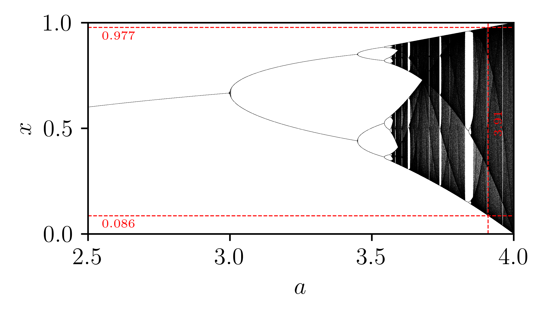
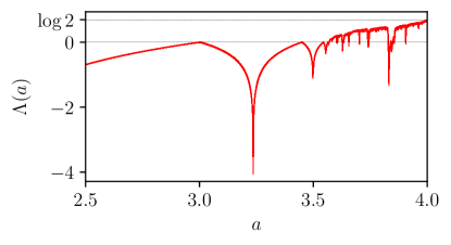
Figure 1: (top)) Bifurcation diagram for logistic map for control parameter $a\in[2.5,4.0]$ and (bottom) Lyapunov exponent $\Lambda(a)$. Observe bifurcations, period doubling, $2^{k}$–cycles, periodic windows, Sharkovskii order, three-implies-chaos rule and transition to full chaos at $a=4$. Values of the parameter $a$ marked by short vertical lines were used to obtain results on the matrix version of the map.

In the limiting case, $a=4$, the motion becomes fully chaotic on the interval $I=[0,1]$ with the Lyapunov exponent $\Lambda=\log 2$. A nonlinear change of the variables allows one to bring this equation to the tent map, which implies that the invariant measure of the corresponding transition operator is given by the so called arc-sin law,

$$\mu_{4}^{*}(x)=\frac{1}{\pi\sqrt{x(1-x)}}$$ (2)

– see e.g. Ott .

Matrix logistic map: Hermitian matrices. To extend the logistic map (1) for the space of hermitian matrices of order $N$, we need to bound the support of spectrum of a given positive hermitian matrix $H=H^{\dagger}\geq 0$. Rescaling the matrix by its operator norm, $||H||_{\rm op}$, equal to the largest eigenvalue $\lambda_{\rm max}$, we obtain the matrix $H_{0}=H/\lambda_{\rm max}$ with spectrum contained in the unit interval, $I=[0,1]$. This matrix can be used as a starting point for the following matrix logistic map,

$$H_{t+1}=f_{a}(H_{t})\ :=\ aH_{t}({\mathbb{I}}-H_{t}),$$ (3)

which acts in the set hermitian matrices with spectrum supported on the unit interval.

Any hermitian matrix can be diagonalized by a unitary transformation, $H_{t}=UD_{t}U^{\dagger}$, where $D_{t}$ denotes a diagonal matrix with eigenvalues of $H_{t}$ at the diagonal. Inserting this form into Eq. (3) we see that the matrix $U$ of eigenvectors of $H_{0}$ is preserved, so the logistic dynamics concerns the eigenvalues only,

$$D_{t+1}=f(D_{t})\ :=\ aD_{t}({\mathbb{I}}-D_{t})=a(D_{t}-D_{t}^{2}).$$ (4)

Thus, the matrix logistic map (3) applied to a given matrix $H_{0}$ of order $N$ can be interpreted as a parallel iteration of $N$ individual initial points, corresponding to the eigenvalues of $H_{0}$ by the scalar map (1). As any continuous measure $\nu$ on the interval $I$ iterated by the Markov operator $M_{a}$, associated with the logistic map (1), is known to converge to the limiting invariant measure $\mu_{a}^{*}=M_{a}\mu_{a}^{*}$, see LM94 , we arrive at the following statement.

Proposition 1.

Consider an ensemble of random Hermitian matrices of order $N$ with spectral density given by any continuous function supported in the unit interval. Iterating its elements $t$ times by the logistic matrix map (3) one obtains asymptotically an ensemble with spectral density converging in the limit $t\to\infty$ to the invariant measure $\mu_{a}^{*}$ of the logistic map (1) with parameter $a$.

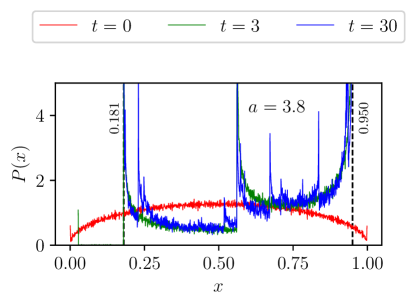
(a)

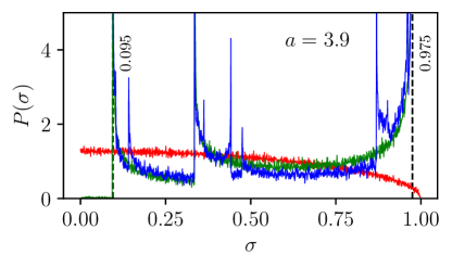
(b)

Figure 2: Spectral distribution $P(y)$ of the rescaled GUE ensemble of size $N=1000$ iterated by the logistic map for $a=3.8$ at times $t=0$ – initial density equivalent to a shifted Wigner semicircle (red), $t=3$ iterations (green), and $t=30$ iterations approximating the invariant measure $\mu_{3.8}^{*}$ (blue). b) Similar plot for dynamics of distribution $P(x)$ of singular values of the rescaled random Ginibre matrices, iterated by the logistic map with parameter $a=3.9$. Initial distribution of Marchenko–Pastur converges to fractal measure $\mu_{3.9}^{*}$. The black dashed lines mark the support of the fractal measures $\mu_{a}^{*}$.

Selecting values of the logistic parameter $a$ such that the invariant measure $\mu_{a}^{*}$ is known to display fractal properties we construct an ensemble of random hermitian matrices with such a spectral distribution. Fast convergence of the initial semicircle density, corresponding to the Gaussian unitary ensemble (GUE) Me04 , to a fractal measure $\mu_{a}^{*}$ determined by the logistic parameter $a$ is visualized in Fig. 2a. In the limiting case of $a=4$, corresponding to the chaotic dynamics in the entire interval, the invariant measure becomes continuous and is given by the arcsine law (2).

Note also that iterating a single random matrix $H$ of size $N$, the spectrum of the matrix $f_{a}^{t}(H)$ is described, in the limit of large matrix dimension, $N\to\infty$, by the invariant measure $\mu_{a}^{*}$.

Matrix logistic map: non-Hermitian matrices. Consider an arbitrary matrix $X$ of order $N$. Using the standard singular value decomposition we write $X=UEV^{\dagger}$, where the diagonal matrix $E$ contains singular values $X$, equal to square roots of eigenvalues of the positive matrix $\sigma_{i}(X)=\sqrt{\lambda_{i}(XX^{\dagger})}$, with $i=1,\dots,N$. Unitary matrices $U$ and $V$ are formed by eigenvectors of hermitian matrices, $XX^{\dagger}$ and $X^{\dagger}X$, respectively. The spectral norm of $X$ is defined by its largest singular value, $||X||_{sp}=\sigma_{\rm max}(X)$.

One can rescale $X$ by its operator norm and arrive at the matrix $X_{0}=X/\sigma_{\rm max}$ with all singular values belonging to the unit interval $I$. To get a direct analogue of the matrix map (3) one can write $X_{1}=aU[E({\mathbb{I}}-E)]V^{\dagger}$, where $U,V$ and $E$ are determined by the singular value decomposition, $X_{0}=UEV^{\dagger}$. The bases fixed by the unitaries $U$ and $V$ remain invariant under the time evolution, hence the proposed variant of the logistic map for an arbitrary normalized non-hermitian matrix $X_{0}=UEV^{\dagger}$ reads

$$X_{t+1}=f(X_{t})\ :=\ a\bigl{[}X_{t}({\mathbb{I}}-VU^{\dagger}X_{t})\bigr{]}.$$ (5)

It is easy to see that if the initial matrix $X$ is hermitian, it can be diagonalized unitarily, $X=UEU^{\dagger}$, so $U^{\dagger}=V^{\dagger}$ and Eq.(5) reduces to Eq.(3).

In the general, non-hermitian case, both unitary matrices $U$ and $V$ of eigenvectors are fixed during the time evolution, as the map (5) acts only on the singular values of $X$. Their dynamics is then governed by the scalar logistic map (1), so we obtain a statement analogous to Proposition 1.

Proposition 2.

Consider an arbitrary ensemble of random (non–hermitian) matrices of order $N$ with the density of singular values described by any continuous function supported in the unit interval. Iterating its elements $t$ times by the matrix map (5) one obtains asymptotically an ensemble with the density of singular values converging in the limit $t\to\infty$ to the invariant measure $\mu_{a}^{*}$ of the logistic map (1).

Evolution of the asymptotic density $P(x)$ of singular values of rescaled random Ginibre matrices Me04 of size $N=1000$ under the action of logistic map (5) with $a=3.9$ is presented in Fig. 2b. Observe a fast convergence of the initial quarter-circle law to the fractal invariant measure $\mu_{3.9}^{*}$.

Coupled logistic map related to a graph. We shall consider here a more general form of Eq. (3), in which the scalar parameter $a$ is replaced by a fixed positive matrix $A=BB^{\dagger}$, so the manifestly positive, matrix logistic map reads,

$$H_{t+1}=f_{B}(H_{t})=BH_{t}(\mathbb{I}-H_{t})B^{\dagger}.$$ (6)

In this setup we easily recover Eq. (3) by setting $B=\sqrt{a}\mathbb{I}$. The simplest case of the model with matrices $B$ of size $N=2$ is discussed in Appendix A.

To demonstrate key features of this model we study matrix $B$ with the structure determined by the adjacency matrix of any directed graph with $N$ vertices. The first one is a linear graph, presented in Fig. 3a and the other one has a structure of the star graph with multiple layers shown in Fig. 4a. In the first case of the graph with four vertices the matrix reads

$$B=B_{4}=\begin{pmatrix}\sqrt{a_{0}}&\sqrt{\varepsilon}&0&0\\ 0&\sqrt{a_{1}}&\sqrt{\varepsilon}&0\\ 0&0&\sqrt{a_{2}}&\sqrt{\varepsilon}\\ 0&0&0&\sqrt{a_{3}}\end{pmatrix},$$ (7)

where $\varepsilon\geq 0$ is a coupling parameter and one needs to ensure that the eigenvalues $\lambda$ of $A=B_{4}B_{4}^{\dagger}$ belong to the interval $[0,4]$.

Models described by these coupling matrices $B$ can be viewed as coupled logistic maps with interaction determined by a graph. We analyzed both systems numerically, in each case performing two tests for chaos. First, we calculate the Lyapunov characteristic exponents (LCE) $\Lambda_{i}$ associated with dynamics $x_{i}$ at the vertices $v_{i}$ of the graphs, making use of the numerical techniques described in BGGS80 ; Ka94 ; Sko10 . Secondly, we perform the 0-1 test for chaos gottwald20160 . In both cases we set $a_{1}=3.91$ and $a_{i}=2.5$ for all $i>1$, which imply chaotic dynamics at $v_{1}$ and regular one at all other vertices $v_{i}$ – see Fig.1.

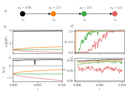
Figure 3: Coupled logistic map corresponding to a linear, four-vertex directed graph – see panel a). Uncoupled system exhibits chaotic dynamics at the black vertex $v_{1}$ determined by the parameter $a_{1}=3.91$ and regular dynamics ($a_{i}=2.5$) at color vertices $v_{2},v_{3},v_{4}$. Quantities describing the system plotted as a function of the coupling strength $\varepsilon$: b) ordered eigenvalues $\lambda_{i}$ of the coupling matrix $A=BB^{\dagger}$; c) Lyapunov exponents $\Lambda_{i}(a)$ corresponding to the uncoupled logistic map (1) with parameter $a=\lambda_{i}$; d) value $K$ of the $0-1$ chaos test; e) Four Lyapunov exponents $\Lambda_{i}$ for the entire $N=4$ dimensional dynamical system (6). The further the vertex $v_{i}$ is situated from the chaotic dynamics at vertex $v_{1}$, the larger value of the coupling parameter $\varepsilon$ is necessary to generate chaotic dynamics at $v_{i}$.

Results obtained for a positive value $\varepsilon$ confirm the transfer of chaotic dynamics between the vertices of the graph due to the coupling between subsystems. Increasing the constant $\varepsilon$, which couples the chaotic dynamics at the vertex $v_{1}$ with other vertices, one observes that the transition to chaos occurs first at the nearest neighbor $v_{2}$, while subsequent vertices $v_{3}$ and $v_{4}$ display chaos only for significantly larger values of $\varepsilon$.

To further drive our point about the transfer of chaos, we present numerical results for the star-shaped graph shown in Fig. 4. As in the case of a linear graph we see the chaotic behavior appearing as a function of the distance from the chaotic vertex. Note that for two vertices with the same distance from the chaotic vertex $v_{1}$, the transfer to chaos occurs for the same value of the coupling $\varepsilon$.

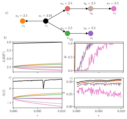
Figure 4: Coupled logistic maps on a seven-vertex star graph a) with chaotic dynamics, at the central vertex $v_{1}$ (in black) determined by logistic parameters $a_{1}=3.91$ and regular dynamics at other vertices $v_{i}$ with $a_{i}=2.5$, for $i=2,\dots 7$. Changes of the dynamics with coupling parameter $\varepsilon$ for $N=7$ dimensional system shown in panels b)-e) presented as in Fig. 3. The transfer to chaos for vertices $v_{2},v_{3}$ and $v_{4}$ directly coupled with $v_{1}$ occurs for the same value of $\varepsilon$. A stronger coupling is needed to induce chaotic dynamics at vertices $v_{5}$ and $v_{6}$. Dynamics at vertex $v_{7}$, more distant from the source of chaos $v_{1}$, becomes chaotic for even larger values of $\varepsilon$.

Concluding Remarks. In this work we introduced a matrix version of the celebrated logistic map, $x^{\prime}=ax(1-x)$, fundamental in studies of chaotic dynamics St00 ; AD06 . In the first step we allowed the variable $x$ to be replaced by a hermitian matrix $H$ of a fixed size $N$ satisfying $0\leq H\leq{\mathbb{I}}$. This assumption leads to a significantly generalized version (3) of the model and introduces novel ensembles of random matrices, which asymptotically (in size $N$ and time $t$) display singular fractal level distributions. In a more general set-up of matrix logistic map acting on non-hermitian matrices (5) the eigenvalues of the asymptotic ensemble form a ring in the complex plane consistent with the “single ring theorem” FZ97 ; GKZ11 , even though the asymptotic distribution of the singular values is fractal – see Fig. 2.

In the second step we assumed that the logistic parameter $a$ is replaced by a positive matrix $A=BB^{\dagger}$ of a fixed order $N$. Defining $B$ to be the adjacency matrix of a given directed graph $\Gamma$ with $N$ vertices we find a related logistic map (6) acting on matrices of order $N$. Each vertex of $\Gamma$ represents a scalar logistic map, while the interactions between the maps are determined by the edges of $\Gamma$. In this way we arrive at a versatile tool to analyze dynamics in complex networks and demonstrate transfer of chaos between subsystems corresponding to particular vertices of the graph. Proposed matrix model is wide enough that it can be also used to mimic nonlinear quantum processes, as the iterated positive matrix can be interpreted as a quantum state subjected to non-linear evolution.

Appendix A $N=2$: Invariant measures for two matrix-coupled logistic maps

In this Appendix we analyze the matrix logistic map in the simplest case of $N=2$. Consider first the map (6) with a diagonal matrix $B=\mathrm{diag}(\sqrt{a_{1}},\sqrt{a_{2}})$. This assumption corresponds to two decoupled logistic maps. The resulting steady state distribution is a convex combination of the steady state distributions for parameters $a_{1}$ and $a_{2}$. Such an example is provided in Fig 5.

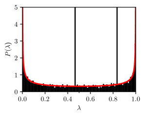
Figure 5: Invariant measure of two decoupled logistic maps, obtained by setting $\varepsilon=0$ in Eq. (6) for $N=2$ with parameters $a_{1}=10/3$ and $a_{2}=4$ forms a combination of both invariant measures of the logistic map (1): superposition of two Dirac measures $\delta(x-x_{\pm})$ localized at $x_{\pm}=\frac{13\pm\sqrt{13}}{20}$ corresponding to $a=a_{1}$ and the continuous arcsine distribution (2) obtained for $a=a_{2}$.

The second example features a richer behavior two logistic maps coupled by a non-diagonal matrix $B$. The coupling is achieved using the matrix $B=\begin{pmatrix}\sqrt{2\sqrt{10/3}}&\sqrt{2/3(11-2\sqrt{30})}\\ 0&\sqrt{2\sqrt{10/3}}\end{pmatrix}$. This gives us the eigenvalues of $A=BB^{\dagger}$ equal to $\lambda_{1}=10/3$ and $\lambda_{2}=4$. The resulting steady-state measure is shown in Fig 6. Note that due to the positive coupling parameter $\varepsilon>0$ the invariant density differs from the combination of of invariant densities for the maps with parameters determined by both eigenvalues of $A$, i.e. $a_{1}=\lambda_{1}=10/3$ and $a_{2}=\lambda_{2}=4$.

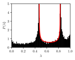
Figure 6: Examplary coupled matrix logistic maps with $N=2$ subsystems. The coupling is achieved by setting to Eq. (6) matrix $B$ with parameters, $a_{1}=a_{2}=1/\sqrt{60+11\sqrt{30}}$ and $\varepsilon=(5/3)^{1/4}2^{3/4}$. This choice implies that the distinct eigenvalues of $BB^{\dagger}$ read $\lambda_{1}=10/3$ and $\lambda_{2}=4$. Observed singularities of the invariant measure at $x_{\pm}=(13\pm\sqrt{13})/{20}$ correspond to fixed points of the logistic map (1) with $a=\lambda_{1}=10/3$. Red curve represents the rescaled arcsin distribution (2) which approximates the part of the distribution between both singularities.

Appendix B Asymptotic eigenvalues of random non-normal matrices

In this section we consider the limiting eigenvalue distribution of matrices $X=UP$, where $P$ is a positive matrix with limiting eigenvalue distribution $\nu_{P}(x)$ and $U$ is a Haar random unitary.

In order to study such matrices, we recall some facts about the S-transform, which was introduced in free random probability by Voiculescu Vo89 . Let us consider a Hermitian matrix $H$. We define its Cauchy transform (Green’s function) as

$$G_{H}(z)=\lim_{N\to\infty}\frac{1}{N}\langle\Tr(z\mathbb{I}-H)^{-1}\rangle=\int\frac{\nu_{H}(x)}{z-x}\differential x.$$ (8)

The Green’s function is related to moments $m_{Hk}$ of $\nu_{H}$

$$G_{H}(z)=\sum_{k=0}^{\infty}\frac{m_{Hk}}{z^{k+1}}.$$ (9)

A more convenient generating function, given by a power series in $z$ rather than in $1/z$ is

$$\psi_{H}(z)=\frac{1}{z}G_{H}\left(\frac{1}{z}\right)-1=\sum_{k=1}^{\infty}m_{Hk}z^{k}.$$ (10)

Let us denote by $\chi_{H}(z)$ the inverse of $\psi_{H}(z)$

$$\chi_{H}(\psi_{H}(z))=\psi_{H}(\chi_{H}(z))=z,$$ (11)

which can be expressed as a power series in $z$ provided that $m_{H1}\neq 0$. The S-transform of $H$ is related to $\chi_{H}$ as

$$S_{H}(z)=\frac{1+z}{z}\chi_{H}(z).$$ (12)

Now we can recall the seminal result by Haagerup and Larsen HL00 , which implies that the limiting eigenvalue distribution of $X$, $\varrho_{X}(z,\overline{z})$, is radially symmetric and related to the S-transform of $P^{2}$,

$$S_{P^{2}}(F_{X}(r)-1)=\frac{1}{r^{2}},$$ (13)

where $F_{X}(r)$ is the radial cumulative density function of the eigenvalues of $X$

$$F_{X}(r)=\int_{|z|\leq r}\varrho_{X}(z,\overline{z})\differential^{2}z=2\pi\int_{0}^{r}s\nu_{X}(s)\differential s=\int_{0}^{r}p_{X}(s)\differential s.$$ (14)

It is related to the eigenvalue density $\varrho_{X}(z,\overline{z})=\mu_{X}(|z|)$. The integrand $p_{X}(s)\differential s=2\pi s\nu_{X}(|z|)$ can be interpreted as the probability of finding the eigenvalues of $X$ in a ring of radii $|z|$ and $|z|+\differential|z|$,

$$p_{X}(r)=\partial_{r}F_{X}(r).$$ (15)

Furthermore, the Haagerup-Larsen theorem tells us that the support of the eigenvalue density of $X$ is a single ring bounded by circles of radii

$$R^{2}_{\rm max}=\int_{0}^{\infty}x\nu_{P^{2}}(x)\differential x,\;\;R^{-2}_{\rm min}=\int_{0}^{\infty}x^{-1}\nu_{P^{2}}(x)\differential x.$$ (16)

Now we have all the ingredients to study the stationary eigenvalue densities of non-normal matrices evolved according to the matrix logistic map (5).

B.1 Fixed point dynamics for logistic parameter $a<3$

In this regime there is a single stationary value for the logistic map, $x_{c}$. Hence $\nu_{P}(x)=\delta(x-x_{c})$ and $X=x_{c}U$ and the eigenvalue density is supported on a circle of radius $x_{c}$

$$p_{X}(r)=\delta(r-x_{c}).$$ (17)

An example of this distribution along with marginal distributions are shown in Fig. 7. This was obtained by iterating 1000 initial matrices of size $N=1000$ for 100 steps and obtaining the final eigenvalues.

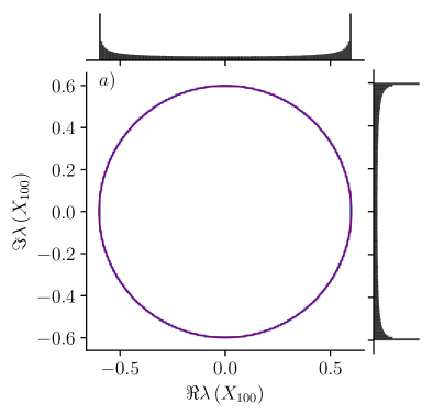
Figure 7: Distribution of eigenvalues of matrix $X_{100}$ obtained by iterating $100$ times a random Ginibre matrix $X_{0}$ of dimension $N=1000$ by the matrix logistic in the case of a single fixed-point, $a=2.5$. The side plots are the marginal distributions of the real and imaginary parts. The distribution is supported on a circle of radius .

B.2 Intermediate dynamics for logistic parameter $3\leq a\leq a_{c}$

In the parameter range, for $a<a_{c}\approx 3.569$, the dynamics is periodic and a sequence of period doubling effects occur while increasing $a$. In the case the logistic map (1) has exactly two fixed points, the invariant measure is formed by a combination of two Dirac delta functions, $\nu_{P}(x)=\frac{1}{2}\delta(x-\alpha_{+})+\frac{1}{2}\delta(x-\alpha_{-})$ and $\alpha_{+}>\alpha_{-}>0$. Assume than that the singular values of a non-Hermitian matrix $X=UP$ is given by such a combination of Dirac deltas. The resulting radial density $p_{X}(r)$ of complex eigenvalues of $X$ reads

$$p_{X}(r)=r\left(\frac{\alpha_{+}^{2}}{(\alpha_{+}^{2}-r^{2})^{2}}+\frac{\alpha_{-}^{2}}{(\alpha_{-}^{2}-r^{2})^{2}}\right).$$ (18)

This distribution is obtained by following the steps described in the previous section and calculating an explicit form of Eq. (15).

The support is a disc of radii

$$r_{\rm min}=\frac{\sqrt{2}\alpha_{+}\alpha_{-}}{\sqrt{\alpha_{+}^{2}+\alpha_{-}^{2}}},\;\;r_{\rm max}=\frac{\sqrt{\alpha_{+}^{2}+\alpha_{-}^{2}}}{\sqrt{2}}.$$ (19)

Let us look at a specific example. Set $=10/3$, then $\alpha_{+}=\frac{13+\sqrt{13}}{20}$, $\alpha_{-}=\frac{13-\sqrt{13}}{20}$. We get

$$r_{\rm min}=\frac{3}{5}\sqrt{\frac{13}{14}}\approx 0.578,\;\;r_{\rm max}=\frac{1}{10}\sqrt{\frac{91}{2}}\approx 0.675.$$ (20)

Again, we show of this distribution in Fig. 8. As before, this was obtained by iterating 1000 initial matrices of size $N=1000$ for 100 steps and obtaining the final eigenvalues.

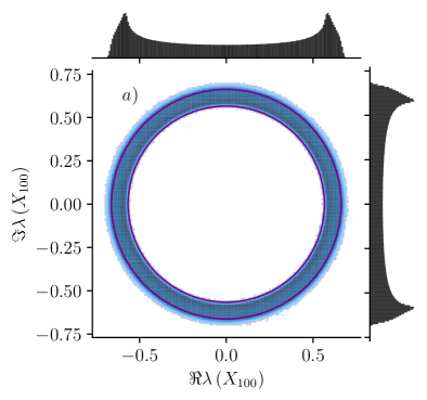
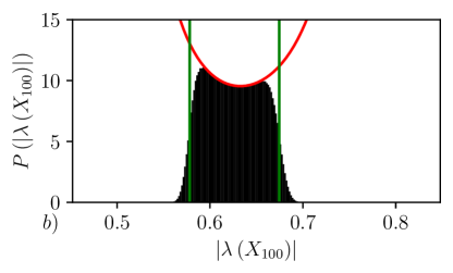
Figure 8: (top) Distribution of eigenvalues of matrix $X_{100}$ obtained by iterating $100$ times a random Ginibre matrix $X_{0}$ of dimension $N=1000$ by the matrix logistic map with $a=10/3$, two fixed-points. The side plots are the marginal distributions of the real and imaginary parts. The circles mark the edges of the disc of the radii from (20). (bottom) Plot showing the distribution of the absolute values of the eigenvalues of $X_{100}$. The green lines mark the support of the asymptotic distribution, the red line represents dsitribution (18).

B.3 Chaotic dynamics for logistic parameter $a=4$

In the fully chaotic case, $a=4$ the invariant measure $\nu_{P}(x)$ is given by the arcsine law (2) – see e.g. Ott . Assuming that the singular values of a non-hermitian matrix $X$ are distributed according to this law, we apply now Eq. (B7) and (B8) to derive the resulting radial density $p_{X}(r)$. It is supported on $[0,\sqrt{3/8}]$ and given by a derivative,

$$\begin{split}p_{X}(r)=&\frac{\partial}{\partial r}\left[-\frac{r^{2}+1}{4\left(r^{2}-1\right)}+\frac{1}{2}\sqrt{T(r)+\frac{Q(r)}{W(r)}}+\right.\\ &\left.-\frac{1}{2}\sqrt{2T(r)+\frac{r^{2}+1}{4\left(1-r^{2}\right)\sqrt{T(r)+\frac{Q(r)}{W(r)}}}-\frac{Q(r)}{W(r)}}\right],\end{split}$$ (21)

with

$$\begin{split}T(r)=&\frac{3r^{4}-2r^{2}+3}{12\left(r^{2}-1\right)^{2}},\\ Q(r)=&4r^{2}(3r^{4}-5r^{2}+3)+\left[U(r)\right]^{2/3},\\ W(r)=&6(r^{2}-1)^{2}\left[U(r)\right]^{1/3},\\ U(r)=&R(r)+27r^{10}-72r^{8}+98r^{6}-72r^{4}+27r^{2},\\ R(r)=&3\sqrt{3}\sqrt{r^{4}\left(r^{2}-1\right)^{6}\left(27r^{4}-46r^{2}+27\right)}.\end{split}$$ (22)

This asymptotic probability distribution describes well numerical results for the radial distribution of complex eigenvalues obtained by iteration of random Ginibre (non-hermitian) matrices of size $N=1000$ – see Fig. 9.

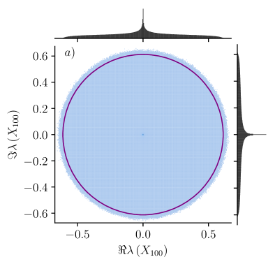
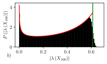
Figure 9: (top) Distribution of eigenvalues of matrix $X_{100}$ obtained by iterating $100$ times a random Ginibre matrix $X_{0}$ of dimension $N=1000$ by the matrix logistic map in the fully chaotic case, $a=4$. The side plots are the marginal distributions of the real and imaginary parts. The circles mark the edges of the disc of the radii from (20). (bottom) Plot showing the distribution of the absolute values of the eigenvalues of $X_{100}$. The green line marks the support of the asymptotic distribution, the red line represents distribution (21).

References

- (1) S.H. Strogatz, Nonlinear dynamics and chaos: with applications to physics, biology, chemistry, and engineering, Perseus Publishing, Cambridge, 2000.
- (2) R. M. May, Simple mathematical models with very complicated dynamics, Nature 261, 459 (1976).
- (3) M. Ausloos and M. Diricks (Eds.), The Logistic Map and the Route to Chaos, Springer-Verlag, Berlin 2006
- (4) M. J. Feigenbaum, Quantitative universality for a class of nonlinear transformations, J. Stat. Phys. 19, 25 (1978).
- (5) A. N. Sharkovskii, Co-existence of cycles of a continuous mapping of the line into itself, Ukrainian Math. J. 16, 61 (1964).
- (6) A. Lasota and M. C. Mackey, Chaos, Fractals and Noise, Springer, 1994.
- (7) T.-Y. Li and J. A. Yorke, Period three implies chaos, Am. Math. Mont. 82, 985 (1975).
- (8) K. Kaneko, Theory and applications of coupled map lattices, Wiley, New York, 1993.
- (9) C. Anteneodo, A. M. Batista and R.L. Viana, Synchronization threshold in coupled logistic map lattices, Physica D 223, 270 (2006).
- (10) A. C. Marti, C. Masoller, Delay-induced synchronization phenomena in an array of globally coupled logistic maps, Phys. Rev. E 67, 056219 (2003).
- (11) A. V. Mahajan and P. M. Gade, Stretched exponential dynamics of coupled logistic maps on a small-world network, J. Stat. Mech. 2018, 023212 (2018).
- (12) L. A. Bunimovich and Ya. G. Sinai, Spacetime chaos in coupled map lattices, Nonlinearity 1, 491 (1988).
- (13) A. Ferretti and N.K. Rahman, A study of coupled logistic map and its applications in chemical physics, Chem. Phys. 119, 275 (1988).
- (14) A. Lloyd, The Coupled Logistic Map: A Simple Model for the Effects of Spatial Heterogeneity on Population Dynamics, J. Theor. Biol. 173, 217 (1995).
- (15) B. E. Kendall and G. A. Fox, Spatial Structure, Environmental Heterogeneity, and Population Dynamics: Analysis of the Coupled Logistic Map, Theor. Popul. Biol. 54, 11 (1998).
- (16) Z. Navickas, R. Smidtaite, A. Vainoras and M. Ragulskis, The logistic map of matrices, Discrete Cont. Dynam. Systems, B 16, 927 (2011).
- (17) Z. Navickas, M. Ragulskis, A. Vainoras and R. Smidtaite, The explosive divergence in iterative maps of matrices Commun. Nonlinear Sci. Numer. Simulat. 17, 4430 (2012).
- (18) R. Smidtaite, Z. Navickas and M. Regulskis, Clocking divergence of iterative maps of matrices, Commun. Nonlinear Sci. Numer. Simulat. 95, 105589 (2021).
- (19) A. Bendersky, J. P. Paz and M. Terra-Cunha, General theory of measurement with two copies of a quantum state, Phys. Rev. Lett. 103, 040404 (2009).
- (20) H. Bechman-Pasquinucci, B. Huttner, and N. Gisin, Phys. Lett. A 242, 198 (1998).
- (21) L. Hardy and D. D. Song, Nonlinear qubit transformations, Phys. Rev. A 64, 032301 (2001).
- (22) J. Feinberg and A. Zee, Non-Gaussian non-Hermitian random matrix theory: phase transition and addition formalism, Nuclear Phys. B 501, 643 (1997).
- (23) A. Guionnet, M. Krishnapur, O. Zeitouni, The single ring theorem, Annals of Mathematics 174, 1189 (2011).
- (24) D. V. Voiculescu, Multiplication of certain non-commuting random variables, J. Operator Theory 18, 223 (1987).
- (25) M. L. Mehta, Random Matrices, III ed. (Academic, New York, 2004).
- (26) E. Ott, Chaos in Dynamical Systems, II ed. CUP, Cambridge 2002
- (27) R.L. Walsworth et. al., Phys. Rev. Lett. 64, 2599 (1990).
- (28) P.K. Majumder et. al., Phys. Rev. Lett. 65, 2931 (1990).
- (29) A. Peres, Phys. Rev. Lett. 63, 1114 (1989).
- (30) N. Gisin, Phys. Lett. A 113, 1 (1990).
- (31) D. R. Terno, Nonlinear operations in quantum-information theory, Phys. Rev. A 59, 3320 (1999).
- (32) I. Bengtsson, K. Życzkowski, Geometry of Quantum States, 2nd ed., (Cambridge University Press, Cambridge, 2017)
- (33) U. Haagerup, F. Larsen, Brown’s spectral distribution measure for -diagonal elements in finite von Neumann algebras, J. Funct. Anal. 176, 331 (2000).
- (34) G. Benettin, L. Galgani, A. Giorgilli, and J. M. Strelcyn, Lyapunov characteristic exponents for smooth dynamical systems and for Hamiltonian systems: A method for computing all of them. Part 2: Numerical application. Meccanica, March:21–30 (1980).
- (35) H. Kantz, A robust method to estimate the maximal Lyapunov exponent of a time series, Phys. Let. A185, 77 (1994).
- (36) C. Skokos, The Lyapunov characteristic exponents and their computation, Lect. Notes Phys. 790, 63 (2010).
- (37) G. A. Gottwald, I. Melbourne, The 0-1 test for chaos: A review, Lecture Notes in Physics 915, 221 (2016).