We assess the impact of top quark production at the LHC on global analyses of parton distributions (PDFs) and of Wilson coefficients in the SMEFT, both separately and in the framework of a joint interpretation. We consider the broadest top quark dataset to date containing all available measurements based on the full Run II luminosity. First, we determine the constraints that this dataset provides on the large-$x$ gluon PDF and study its consistency with other gluon-sensitive measurements. Second, we carry out a SMEFT interpretation of the same dataset using state-of-the-art SM and EFT theory calculations, resulting in bounds on 25 Wilson coefficients modifying top quark interactions. Subsequently, we integrate the two analyses within the SIMUnet approach to realise a simultaneous determination of the SMEFT PDFs and the EFT coefficients and identify regions in the parameter space where their interplay is most phenomenologically relevant. We also demonstrate how to separate eventual BSM signals from QCD effects in the interpretation of top quark measurements at the LHC.

1 Introduction

The top quark is one of the most remarkable particles within the Standard Model (SM). Being the heaviest elementary particle known to date, with a mass around 185 times heavier than a proton, and the only fermion with an $\mathcal{O}(1)$ Yukawa coupling to the Higgs boson, the top quark has long been suspected to play a privileged role in potential new physics extensions beyond the Standard Model (BSM). For instance, radiative corrections involving top quarks are responsible for the so-called hierarchy problem of the SM, and the value of its mass $m_{t}$ determines whether the vacuum state of our Universe is stable, metastable, or unstable [1, 2, 3]. For these reasons, since its discovery at the Tevatron in 1995 [4, 5] the properties of the top quark have been scrutinised with utmost attention and a large number of BSM searches involving top quarks as final states have been carried out. The focus on the top quark has further intensified since the start of operations at the LHC, which has realised an unprecedented top factory producing more than 200 million top quark pairs so far, for example.

In addition to this excellent potential for BSM studies, top quark production at hadron colliders also provides unique information on a variety of SM parameters such as the strong coupling constant $\alpha_{s}(m_{t})$ [6, 7], the CKM matrix element $V_{tb}$ [8], and the top quark mass $m_{t}$ [9, 10], among several others. Furthermore, top quark production at the LHC constrains the parton distribution functions (PDFs) of the proton [11, 12], in particular the large-$x$ gluon PDF from inclusive top quark pair production [13, 14, 15] and the quark PDF flavour separation from inclusive single top production [16, 17]. Indeed, fiducial and differential measurements of top quark pair production are part of the majority of recent PDF determinations. Reliably extracting SM parameters, including those parametrising the subnuclear structure of the proton in the PDFs, from LHC top quark production data has been made possible thanks to recent progress in higher order QCD and electroweak calculations of top quark production. Inclusive top quark pair production is now known at NNLO in the QCD expansion both for single- and double-differential distributions [18, 19], eventually complemented with electroweak corrections [20], threshold resummation [21], and matching to parton showers [22]. NNLO QCD corrections are also known for single top quark production at the LHC, both in the $t$-channel [23, 24] and in the $s$-channel [25].

Even in BSM scenarios where new particles are sufficiently heavy such that direct production lies beyond the reach of the LHC, current and future measurements can still provide BSM sensitivity through low-energy signatures. These are typically revealed in the modification of SM particle properties, such as their interactions and coupling strengths. In this context, a powerful model-agnostic framework to parametrise, identify, and correlate the low-energy signatures of heavy BSM physics is the Standard Model Effective Field Theory (SMEFT). Several groups, both from the theory community and within the experimental collaborations, have presented interpretations of LHC top quark measurements in the SMEFT framework [26, 27, 28, 29, 30, 31, 32, 33] to derive bounds on higher-dimensional EFT operators that distort the interactions of top quarks. A key feature of these analyses is that the unprecedented energy reach of the LHC data increases the sensitivity to SMEFT operators via energy-growing effects entering the partonic cross-sections.

Therefore, in the LHC precision era, top quark measurements are being interpreted in (at least) two frameworks with rather different underlying assumptions. On the one hand, global PDF fits assume the SM and use top data to constrain the PDFs, producing Standard Model PDFs (denoted “SM-PDFs” in the following). On the other hand, SMEFT analyses assume that top data does not modify the SM predictions, and in particular that the proton PDFs are unchanged; we thus refer to SMEFT fits as “fixed-PDF” in the following. The two assumptions cannot be simultaneously correct, and hence one must answer two pressing questions concerning the interpretation of LHC top quark measurements. First, are SM-PDFs contaminated by BSM physics, encapsulated in the SMEFT framework, which are being reabsorbed into the fitted PDF boundary condition? Second, are the results of existing SMEFT interpretations dependent on the choice of PDFs entering the SM calculations, and is it consistent to use PDF sets that already include top quark data? It should be emphasized that for top quark production one cannot classify the data in two disjoint “SM-PDF” and “fixed-PDF” regions, since in both cases sensitivity arises from the high-energy regime.

These two questions can only be answered by means of the simultaneous determination of the PDFs and EFT coefficients from a common input dataset resulting in so-called “SMEFT-PDFs”. A proof of concept of this strategy was presented for deep-inelastic scattering (DIS) data [34] and then extended to a joint analysis of DIS and Drell-Yan (DY) data [35] including projections for the HL-LHC; see also [36, 37, 38] for related work. The studies of [34, 35] were restricted to a small number of representative EFT operators, and extending them to the realistic case of processes sensitive to a large number of operators, such as top or jet production data, required the development of improved techniques. With this motivation, a new methodology dubbed SIMUnet was developed [39] making possible global SMEFT-PDF interpretations of LHC data suitable for processes depending on up to several tens of EFT operators. A key feature of SIMUnet is that it can be easily projected to both the SM-PDF case, in which it reduces to the NNPDF fitting methodology [40, 41], and to the fixed-PDF case, where it becomes equivalent to global EFT fitting tools such as SMEFiT [42].

The aim of this work is to extend the initial explorations of [34, 35] to a global determination of the SMEFT-PDFs from top quark production measurements. To this purpose, we consider the broadest top quark dataset used to date in either PDF or EFT interpretations, which in particular contains all available measurements from ATLAS and CMS based on the full Run II luminosity. By combining this wide dataset with the SIMUnet methodology, we derive bounds on 25 independent Wilson coefficients modifying top quark interactions, identify regions in the parameter space where the interplay between PDFs and SMEFT signatures is most phenomenologically relevant, and demonstrate how to separate eventual BSM signals from QCD effects in the interpretation of top quark measurements. As a non-trivial by-product, we also revisit the SM-PDF and fixed-PDF analyses by quantifying the information that our comprehensive top quark dataset provides. On the one hand, we assess the impact on the large-$x$ gluon (SM-PDF), and on the other, we study the impact on the EFT coefficients (fixed-PDF), and compare our findings with related studies in the literature.

The structure of this paper is as follows. To begin with, in Sect. 2 we describe the data inputs and the theory calculations (both in the SM and in the SMEFT) used in our study, focusing on top quark sector measurements. The SIMUnet methodology deployed for the simultaneous extraction of PDFs and EFT coefficients, including its application to the fixed-PDF and SM-PDF analyses, is reviewed in Sect. 3. Subsequently, in Sect. 4 we present the results of the SM-PDF fits, and in particular we quantify the impact on the large-$x$ gluon of recent high-statistics Run II measurements. In Sect. 5 we consider the fixed-PDF analyses and present the most extensive SMEFT interpretation of top quark data from the LHC to date, including comparisons with previous results in the literature. The main results of this paper are presented in Sect. 6, namely the simultaneous determinations of the PDFs and EFT coefficients and the comparison of these with both the fixed-PDF and SM-PDF cases. We summarise our results and outline some possible future developments in Sect. 7.

Technical details of the analysis are collected in the appendices. App. A provides usage recommendations for interpretations of top quark measurements sensitive both to PDFs and SMEFT coefficients. App. B collects the theory settings for the SMEFT calculations, mainly concerning input schemes and operator definitions. App. C carries out a benchmark comparison between SIMUnet (in the fixed-PDF case) and the public SMEFiT code, demonstrating the agreement between the two frameworks at the linear level. The fit quality to the datasets considered in the analysis is presented in App. D, and representative data-theory comparisons are given. Finally, in App. E we discuss the difficulties in extending the simultaneous analysis of PDFs and EFT coefficients to the case where terms quadratic in the EFT Wilson coefficients are dominant.

2 Experimental data and theory calculations

We begin by describing the experimental data and theoretical predictions, both in the SM and in the SMEFT, used as input for the present analysis. We start in Sect. 2.1 by describing the datasets that we consider, with emphasis on the top quark production measurements. Then in Sect. 2.2 we use a modified version of the selection criteria defined in [40] to determine a maximally consistent dataset of top quark data to be used in the subsequent PDF and SMEFT interpretations. Finally, in Sect. 2.3 we describe the calculation settings of the SM and SMEFT cross-sections for top quark processes, pointing the reader to the appendices for the technical details of their implementation.

2.1 Experimental data

With the exception of the top quark measurements, the dataset used in this work for fitting the PDFs both in the SM-PDF and SMEFT-PDF cases overlaps with that of the NNPDF4.0 determination presentend in Ref. [40]. In particular, the no-top variant of the NNPDF4.0 dataset consists of 4535 data points corresponding to a wide variety of processes in deep-inelastic lepton-proton scattering [43, 44, 45, 46, 47, 48, 49, 50, 51] and in hadronic proton-proton collisions [52, 53, 54, 55, 56, 57, 58, 59, 60, 61, 62, 63, 64, 65, 66, 67, 68, 69, 70, 71, 72, 73, 74, 75, 76, 77, 78, 79, 80, 81, 82, 83, 84, 85, 86, 87, 88, 89, 90]; see [40] for more details.

Concerning the LHC top quark measurements considered in the present analysis, they partially overlap, but significantly extend, the top datasets included in global PDF fits such as NNPDF4.0  [40] as well as in SMEFT analyses of the top quark sector [91, 42]. Here we discuss in turn the different types of measurements to be included: inclusive $t\bar{t}$ cross sections and differential distributions; $t\bar{t}$ production asymmetries; the $W$-helicity fractions; associated top pair production with vector bosons and heavy quarks, including $\bar{t}tZ$, $\bar{t}tW$, $\bar{t}t\gamma$, $\bar{t}t\bar{t}t$, $\bar{t}t\bar{b}b$; $t-$ and $s-$channel single top production; and associated single top and vector boson production.

Choice of kinematic distribution.

Many of these measurements, in particular those targeting top quark pair production, are available differentially in several kinematic variables, as well as either absolute distributions, or distributions normalised to the fiducial cross-section. We must decide which of the available kinematic distributions associated to a given measurement should be included in the fit, and whether it is more advantageous to consider absolute or normalised distributions.

Regarding the former, we note that correlations between kinematic distributions are in general not available, and only one distribution at a time can be included without double-counting (one exception is the ATLAS $t\bar{t}$ lepton+jet measurement at $\sqrt{s}=8$ TeV [92] where the full correlation matrix is provided). Therefore, wherever possible we include the top-pair invariant mass $m_{t\bar{t}}$ distributions with the rationale that these have enhanced sensitivity to SMEFT operators via energy-growing effects; they also provide direct information on the large-$x$ PDFs. Otherwise, we consider the top or top-pair rapidity distributions, $y_{t}$ and $y_{t\bar{t}}$ respectively, which also provide the sought-for information on the large-$x$ PDFs; furthermore they benefit from moderate higher-order QCD and electroweak corrections [14].

Regarding the choice of absolute versus normalised distributions, we elect to use normalised distributions together with corresponding fiducial cross-sections throughout. Normalised distributions are typically more precise that their absolute counterparts, since experimental and theoretical errors partially cancel out when normalising. In addition, normalisation does not affect the PDF and EFT sensitivity of the measurement, provided the fiducial cross section measurements used for normalising are also accounted for. From the implementation point of view, since in a normalised measurement one bin is dependent on the others, we choose to exclude the bin with lowest $m_{t\bar{t}}$ value (the production threshold) to avoid losing sensitivity arising from the high-energy tails.

Inclusive $t\bar{t}$ production.

Exp.	$\bf{\sqrt{s}}$ (TeV)	Channel	Observable	$\mathcal{L}$ (fb${}^{-1}$)	$\mathbf{n_{\rm dat}}$	Ref.	New (PDF fits)	New (SMEFT fits)
ATLAS	7	dilepton	$\sigma(t\bar{t})$	$4.6$	1	[93]		($\checkmark$)
	8	dilepton	$\sigma(t\bar{t})$	$20.3$	1	[93]		($\checkmark$)
			$1/\sigma d\sigma/dm_{t\bar{t}}$	$20.2$	5	[94]	($y_{t\bar{t}}\rightarrow m_{t\bar{t}}$)	(absolute $\rightarrow$ ratio)
		$\ell+$jets	$\sigma(t\bar{t})$	$20.2$	1	[95]	$\checkmark$	($\checkmark$)
			$1/\sigma d\sigma/d|y_{t}|$	$20.3$	4	[92]		($m_{t\bar{t}},p_{t}^{T}\rightarrow|y_{t}|,|y_{t\bar{t}}|$)
			$1/\sigma d\sigma/d|y_{t\bar{t}}|$	$20.3$	4	[92]		($m_{t\bar{t}},p_{t}^{T}\rightarrow|y_{t}|,|y_{t\bar{t}}|$)
	13	dilepton	$\sigma(t\bar{t})$	$36.1$	1	[96]	$\checkmark$	$\checkmark$
		hadronic	$\sigma(t\bar{t})$	$36.1$	1	[97]	$\checkmark$	$\checkmark$
			$1/\sigma d^{2}\sigma/d|y_{t\bar{t}}|dm_{t\bar{t}}$	$36.1$	10	[97]	$\checkmark$	$\checkmark$
		$\ell+$jets	$\sigma(t\bar{t})$	$139$	1	[98]		($\checkmark$)
			$1/\sigma d\sigma/dm_{t\bar{t}}$	$36$	8	[99]	$\checkmark$	(absolute $\rightarrow$ ratio)
CMS	5	combination	$\sigma(t\bar{t})$	0.027	1	[100]		$\checkmark$
	7	combination	$\sigma(t\bar{t})$	$5.0$	1	[101]		$\checkmark$
	8	combination	$\sigma(t\bar{t})$	$19.7$	1	[101]		$\checkmark$
		dilepton	$1/\sigma d^{2}\sigma/dy_{t\bar{t}}dm_{t\bar{t}}$	$19.7$	16	[102]	($m_{t\bar{t}},y_{t}\rightarrow m_{t\bar{t}},y_{t\bar{t}}$)
		$\ell+$jets	$1/\sigma d\sigma/dy_{t\bar{t}}$	$19.7$	9	[103]
	13	dilepton	$\sigma(t\bar{t})$	$43$	1	[104]		($\checkmark$)
			$1/\sigma d\sigma/dm_{t\bar{t}}$	$35.9$	5	[105]		(absolute $\rightarrow$ ratio)
		$\ell+$jets	$\sigma(t\bar{t})$	$137$	1	[106]	$\checkmark$	$\checkmark$
			$1/\sigma d\sigma/dm_{t\bar{t}}$	$137$	14	[106]	$\checkmark$	$\checkmark$

Table 2.1: The inclusive cross-sections and differential distributions for top quark pair production from ATLAS and CMS that we consider in this analysis. For each dataset, we indicate the experiment, the centre of mass energy $\sqrt{s}$, the final-state channel, the observable(s) used in the fit, the integrated luminosity $\mathcal{L}$ in inverse femtobarns, and the number of data points $n_{\rm dat}$, together with the corresponding publication reference. In the last two columns, we indicate with a $\checkmark$ the datasets that are included for the first time here in a global PDF fit and in a SMEFT interpretation, respectively. The sets marked with brackets have already been included in previous studies but here we account for their constraints in different manner (e.g. by changing spectra or normalisation), as indicated in the table and in the text description.

A summary of the inclusive $t\bar{t}$ fiducial cross sections and differential distributions considered in this work is provided in Table 2.1. We indicate in each case the centre of mass energy $\sqrt{s}$, the final-state channel, the observable(s) used in the fit, the luminosity, and the number of data points $n_{\rm dat}$, together with the corresponding publication reference. In the last two columns, we indicate with a $\checkmark$ the datasets that are included for the first time here in a global PDF fit (specifically, those which are new with respect to NNPDF4.0 ) and in a SMEFT interpretation (specifically, in comparison with the global fits of [91, 42]). The sets marked with brackets have already been included in previous studies, but are implemented here in a different manner (e.g. by changing spectra or normalisation), as indicated in the table; more details are given in each paragraph of the section.

The ATLAS dataset comprises six total cross section measurements and five differential normalised cross section measurements. Concerning the latter, at $8$ TeV we include three distributions from the dilepton and $\ell+$jets channels. In the $\ell+$jets channel, several kinematic distributions are available together with their correlations. Following the dataset selection analysis carried out in [40], we select to fit the $y_{t}$ and $y_{t\bar{t}}$ distributions as done in the NNPDF4.0 baseline. At $13$ TeV, we include the normalised cross sections differential in $m_{t\bar{t}}$ from the $\ell+$jets and hadronic channels, with both measurements being considered for the first time here in the context of a PDF analysis.

Moving to CMS, in the inclusive $t\bar{t}$ category we consider five total cross section and four normalised differential cross section measurements. At $\sqrt{s}=8$ TeV we include differential distributions in the $\ell+$jets and dilepton channels, the latter being doubly differential in $y_{t\bar{t}}$ and $m_{t\bar{t}}$. The double-differential 8 TeV measurement is part of NNPDF4.0 , but there the $(y_{t},m_{t\bar{t}})$ distribution was fitted instead. At $13$ TeV, we include the $m_{t\bar{t}}$ distributions in the dilepton and $\ell+$jets channels. In the latter case we include the single $m_{t\bar{t}}$ distribution rather than the double-differential one in $(m_{t\bar{t}},y_{t\bar{t}})$, which is also available, since we find that the latter cannot be reproduced by the NNLO SM predictions. We present a dedicated analysis of the double-differential distribution in Sect. 5.3. As mentioned above, we will study the impact of our dataset selection choices by presenting variations of the baseline SM-PDF, fixed-PDF, and SMEFT-PDF analyses in the following sections.

$t\bar{t}$ asymmetry measurements.

The $t\bar{t}$ production asymmetry at the LHC is defined as:

$$A_{C}={{N(\Delta|y|>0)-N(\Delta|y|<0)}\over{N(\Delta|y|>0)+N(\Delta|y|<0)}}\,,$$ (2.1)

with $N(P)$ being the number of events satisfying the kinematical condition $P$, and $\Delta|y|=|y_{t}|-|y_{\bar{t}}|$ is the difference between the absolute values of the top quark and anti-top quark rapidities. The asymmetry $A_{C}$ can be measured either integrating over the fiducial phase space or differentially, for example binning in the invariant mass $m_{t\bar{t}}$. Measurements of $A_{C}$ are particularly important in constraining certain SMEFT directions, in particular those associated to the two-light-two-heavy operators. However, they are unlikely to have an impact on PDF fitting due to their large experimental uncertainties; nevertheless, with the underlying motivation of a comprehensive SMEFT-PDF interpretation of top quark data, we consider here the $A_{C}$ measurement as part of our baseline dataset, and hence study whether or not they also provide relevant PDF information. A summary of the asymmetry measurements included in this work is given in Table 2.2.

Experiment	$\bf{\sqrt{s}}$(TeV)	Channel	Observable	$\mathcal{L}$ (fb${}^{-1}$)	$\mathbf{n_{\rm dat}}$	Ref.	New (PDF fits)	New (SMEFT fits)
ATLAS	8	dilepton	$A_{C}$	$20.3$	1	[107]	$\checkmark$
	13	$\ell+$jets	$A_{C}$	$139$	5	[108]	$\checkmark$	$\checkmark$
CMS	8	dilepton	$A_{C}$	$19.5$	3	[109]	$\checkmark$
	13	$\ell+$jets	$A_{C}$	$138$	3	[110]	$\checkmark$
ATLAS & CMS combination	8	$\ell+$jets	$A_{C}$	$20$	6	[111]	$\checkmark$

Table 2.2: Same as Table 2.1 for the $t\bar{t}$ asymmetry datasets.

$W$-helicity fractions.

The $W$-helicity fractions $F_{0},F_{L}$ and $F_{R}$ are PDF-independent observables sensitive to SMEFT corrections, and the dependence of the theory predictions with respect to the Wilson coefficients can be computed analytically. Since these $W$-helicity fractions are PDF-independent observables, to include them in the joint SMEFT-PDF analysis one has to extend the methodology presented in [39] to include in the fit datasets that either lack, or have negligible, PDF sensitivity and depend only on the EFT coefficients. We describe how this can be achieved within the SIMUnet framework in Sect. 3.

In Table 2.3 we list the LHC measurements of the $W$-helicity fractions considered in the current analysis. At $\sqrt{s}=8$ TeV we include the combined ATLAS and CMS measurement from [112], while at $13$ TeV we consider the ATLAS measurement of the $W$-helicities from [113], for the first time in a SMEFT fit.

Experiment	$\bf{\sqrt{s}}$(TeV)	Observable	$\mathcal{L}$ (fb${}^{-1}$)	$\mathbf{n_{\rm dat}}$	Ref.	New (SMEFT fits)
ATLAS & CMS combination	8	$F_{0},F_{L}$	$20$	2	[112]
ATLAS	13	$F_{0},F_{L}$	$139$	2	[113]	$\checkmark$

Table 2.3: Same as Table 2.1 for the $W$-helicity fraction measurements. These helicity fractions are PDF-independent and hence are only relevant in constraining the EFT coefficients.

Associated top quark pair production.

The next class of observables that we discuss is associated $t\bar{t}$ production with a $Z$- or a $W$-boson (Table 2.4), a photon $\gamma$ (Table 2.5), or a heavy quark pair ($t\bar{t}b\bar{b}$ or $t\bar{t}t\bar{t}$, Table 2.6). While measurements of $t\bar{t}V$ have been considered for SMEFT interpretations, we use them for the first time here in the context of a PDF determination. The rare processes $t\bar{t}\gamma$, $t\bar{t}b\bar{b}$, and $t\bar{t}t\bar{t}$ exhibit a very weak PDF sensitivity and hence in the present analysis their theory predictions are obtained using a fixed PDF, in the same manner as the $W$-helicity fractions in Table 2.3.

Exp.	$\bf{\sqrt{s}}$ (TeV)	Observable	$\mathcal{L}$ (fb${}^{-1}$)	$\mathbf{n_{\rm dat}}$	Ref.	New (PDF fits)	New (SMEFT fits)
ATLAS	8	$\sigma(t\bar{t}Z)$	$20.3$	1	[114]	$\checkmark$
		$\sigma(t\bar{t}W)$	$20.3$	1	[114]	$\checkmark$
	13	$\sigma(t\bar{t}Z)$	$36.1$	1	[115]	$\checkmark$
		$1/\sigma d\sigma(t\bar{t}Z)/dp_{T}^{Z}$	$139$	6	[116]	$\checkmark$	$\checkmark$
		$\sigma(t\bar{t}W)$	$36.1$	1	[115]	$\checkmark$
CMS	8	$\sigma(t\bar{t}Z)$	$19.5$	1	[117]	$\checkmark$
		$\sigma(t\bar{t}W)$	$19.5$	1	[117]	$\checkmark$
	13	$\sigma(t\bar{t}Z)$	$35.9$	1	[118]	$\checkmark$
		$1/\sigma d\sigma(t\bar{t}Z)/dp_{T}(Z)$	$77.5$	3	[119]	$\checkmark$	(absolute $\rightarrow$ ratio)
		$\sigma(t\bar{t}W)$	$35.9$	1	[118]	$\checkmark$

Table 2.4: Same as Table 2.1 for the measurements of top quark production in association with a vector boson.

Experiment	$\bf{\sqrt{s}}$(TeV)	Observable	$\mathcal{L}$ (fb${}^{-1}$)	$\mathbf{n_{\rm dat}}$	Ref.	New (SMEFT fits)
ATLAS	8	$\sigma(t\bar{t}\gamma)$	$20.2$	1	[120]
CMS	8	$\sigma(t\bar{t}\gamma)$	$19.7$	1	[121]

Table 2.5: Same as Table 2.1 for $t\bar{t}$ production in association with a photon. Theory predictions for these observables adopt a fixed PDF.

Experiment	$\bf{\sqrt{s}}$(TeV)	Channel	Observable	$\mathcal{L}$ (fb${}^{-1}$)	$\mathbf{n_{\rm dat}}$	Ref.	New (SMEFT fits)
ATLAS	13	multi-lepton	$\sigma_{\text{tot}}(t\bar{t}t\bar{t})$	$139$	1	[122]
		single-lepton	$\sigma_{\text{tot}}(t\bar{t}t\bar{t})$	$139$	1	[123]	$\checkmark$
		$\ell+$jets	$\sigma_{\text{tot}}(t\bar{t}b\bar{b})$	$36.1$	1	[124]
CMS	13	multi-lepton	$\sigma_{\text{tot}}(t\bar{t}t\bar{t})$	$137$	1	[125]
		single-lepton	$\sigma_{\text{tot}}(t\bar{t}t\bar{t})$	$35.8$	1	[126]
		all-jet	$\sigma_{\text{tot}}(t\bar{t}b\bar{b})$	$35.9$	1	[127]
		dilepton	$\sigma_{\text{tot}}(t\bar{t}b\bar{b})$	$35.9$	1	[128]
		$\ell$+jets	$\sigma_{\text{tot}}(t\bar{t}b\bar{b})$	$35.9$	1	[128]	$\checkmark$

Table 2.6: Same as Table 2.1 for the measurements of $t\bar{t}$ production in association with a heavy quark pair. Theory predictions for these observables adopt a fixed PDF.

Concerning the $t\bar{t}Z$ and $t\bar{t}W$ data, from both ATLAS and CMS we use four fiducial cross section measurements at 8 TeV and 13 TeV, and one distribution differential in $p_{T}^{Z}$ at 13 TeV. These measurements are particularly interesting to probe SMEFT coefficients that modify the interactions between the top quark and the electroweak sector. For top-quark production associated with a photon, we include the fiducial cross-section measurements from ATLAS and CMS at 8 TeV; also available is a differential distribution at 13 TeV from ATLAS binned in the photon transverse momentum $p_{T}^{\gamma}$ [129], but we exclude this from our analysis because of the difficulty in producing SMEFT predictions in the fiducial phase space (in the FitMakeranalysis, its inclusion is only approximate, and in SMEFiT this distribution is neglected entirely). Finally, we include fiducial measurements of $t\bar{t}b\bar{b}$ and $t\bar{t}t\bar{t}$ production at 13 TeV considering the data with highest luminosity for each available final state.

Inclusive single-top pair production.

The inclusive single-top production data considered here and summarised in Table 2.7 comprises measurements of single-top production in the $t$-channel, which have previously been included in PDF fits [16, 40], as well as measurements of single-top production in the $s$-channel, which in the context of PDF studies have been implemented for the first time in this study. For $t$-channel production, we consider the ATLAS and CMS top and anti-top fiducial cross sections $\sqrt{s}=7,8,$ and 13 TeV, as well as normalised $y_{t}$ and $y_{\bar{t}}$ distributions at 7 and 8 TeV (ATLAS) and at 13 TeV (CMS). For $s$-channel production, no differential measurements are available and hence we consider fiducial cross-sections at 8 and 13 TeV from ATLAS and CMS.

Exp.	$\bf{\sqrt{s}}$ (TeV)	Channel	Observable	$\mathcal{L}$ (fb${}^{-1}$)	$\mathbf{n_{\rm dat}}$	Ref.	New (PDF fits)	New (SMEFT fits)
ATLAS	7	$t$-channel	$\sigma_{\text{tot}}(t)$	$4.59$	1	[130]	($\checkmark$)	$\checkmark$
			$\sigma_{\text{tot}}(\bar{t})$	$4.59$	1	[130]	($\checkmark$)	$\checkmark$
			$1/\sigma d\sigma(tq)/dy_{t}$	$4.59$	3	[130]		$\checkmark$
			$1/\sigma d\sigma(\bar{t}q)/dy_{\bar{t}}$	$4.59$	3	[130]		$\checkmark$
	8	$t$-channel	$\sigma_{\text{tot}}(t)$	$20.2$	1	[131]	($\checkmark$)	$\checkmark$
			$\sigma_{\text{tot}}(\bar{t})$	$20.2$	1	[131]	($\checkmark$)	$\checkmark$
			$1/\sigma d\sigma(tq)/dy_{t}$	$20.2$	3	[131]		($\checkmark$)
			$1/\sigma d\sigma(\bar{t}q)/dy_{\bar{t}}$	$20.2$	3	[131]		($\checkmark$)
		$s$-channel	$\sigma_{\text{tot}}(t+\bar{t})$	$20.3$	1	[132]	$\checkmark$
	13	$t$-channel	$\sigma_{\text{tot}}(t)$	$3.2$	1	[133]	($\checkmark$)
			$\sigma_{\text{tot}}(\bar{t})$	$3.2$	1	[133]	($\checkmark$)
		$s$-channel	$\sigma_{\text{tot}}(t+\bar{t})$	$139$	1	[134]	$\checkmark$	$\checkmark$
CMS	7	$t$-channel	$\sigma_{\text{tot}}(t)+\sigma_{\text{tot}}(\bar{t})$	$1.17,1.56$	1	[135]		$\checkmark$
	8	$t$-channel	$\sigma_{\text{tot}}(t)$	$19.7$	1	[136]	($\checkmark$)
			$\sigma_{\text{tot}}(\bar{t})$	$19.7$	1	[136]	($\checkmark$)
		$s$-channel	$\sigma_{\text{tot}}(t+\bar{t})$	$19.7$	1	[137]	$\checkmark$
	13	$t$-channel	$\sigma_{\text{tot}}(t)$	$2.2$	1	[138]	($\checkmark$)
			$\sigma_{\text{tot}}(\bar{t})$	$2.2$	1	[138]	($\checkmark$)
			$1/\sigma d\sigma/d|y^{(t)}|$	$35.9$	4	[139]	$\checkmark$

Table 2.7: Same as Table 2.1 for the inclusive single-top production datasets.

Associated single top-quark production with weak bosons.

Finally, Table 2.8 lists the measurements of associated single-top production with vector bosons included in our analysis. We consider fiducial cross-sections for $tW$ production at 8 and 13 TeV from ATLAS and CMS in the dilepton and single-lepton final states, as well as the $tZj$ fiducial cross-section at 13 TeV from ATLAS and CMS in the dilepton final state. In addition, kinematical distributions in $tZj$ production from CMS at 13 TeV are considered for the first time here in an EFT fit. For these differential distributions, the measurement is presented binned in either $p_{T}^{Z}$ or $p_{T}^{t}$; here, we take the former as default for consistency with the corresponding $t\bar{t}Z$ analysis.

Experiment	$\bf{\sqrt{s}}$(TeV)	Channel	Observable	$\mathcal{L}$ (fb${}^{-1}$)	$\mathbf{n_{\rm dat}}$	Ref.	New (SMEFT fits)
ATLAS	8	dilepton	$\sigma_{\text{tot}}(tW)$	$20.3$	1	[140]
		single-lepton	$\sigma_{\text{tot}}(tW)$	$20.2$	1	[141]
	13	dilepton	$\sigma_{\text{tot}}(tW)$	$3.2$	1	[142]
		dilepton	$\sigma_{\text{fid}}(tZj)$	$139$	1	[143]
CMS	8	dilepton	$\sigma_{\text{tot}}(tW)$	$12.2$	1	[144]
	13	dilepton	$\sigma_{\text{tot}}(tW)$	$35.9$	1	[145]
		dilepton	$\sigma_{\text{fid}}(tZj)$	$77.4$	1	[146]
		dilepton	$d\sigma_{\text{fid}}(tZj)/dp_{T}^{t}$	$138$	3	[147]	$\checkmark$
		single-lepton	$\sigma_{\text{tot}}(tW)$	$36$	1	[148]	$\checkmark$

Table 2.8: Same as Table 2.1 for single-top production in association with an electroweak bosons.

2.2 Dataset selection

The top quark production measurements listed in Tables 2.1-2.8 summarise all datasets that have been considered for the present analysis. In principle, however, some of these may need to be excluded from the baseline fit dataset to ensure that the baseline dataset is maximally consistent. Following the dataset selection procedure adopted in [40], here our baseline dataset is chosen to exclude datasets that may be either internally inconsistent or inconsistent with other measurements of the same process type. These inconsistencies can be of experimental origin, for instance due to unaccounted (or underestimated) systematic errors, or numerically unstable correlation models, as well as originating in theory, for example whenever a given process is affected by large missing higher-order perturbative uncertainties. Given that the ultimate goal of a global SMEFT analysis, such as the present one, is to unveil deviations from the SM, one should strive to deploy objective dataset selection criteria that exclude datasets affected by such inconsistencies, which are unrelated to BSM physics.

The first step is to run a global SM-PDF fit including all the datasets summarised in Tables 2.1-2.8 (and additionally a fit with the data summarised therein, but with the CMS measurement of the differential $t\bar{t}$ cross-section at $13$ TeV in the $\ell+$jets channel replaced with the double-differential measurement) and monitor in each case the following two statistical estimators:

• The total $\chi^{2}$ per data point and the number of standard deviations $n_{\sigma}$ by which the value of the $\chi^{2}$ per data point differs from the median of the $\chi^{2}$ distribution for a perfectly consistent dataset,

  $$n_{\sigma}\equiv{{|\chi^{2}-1|}\over{\sigma_{\chi^{2}}}}={{|\chi^{2}-1|}\over{\sqrt{2/n_{\rm dat}}}}\,,$$ (2.2)

  where the $\chi^{2}$ in this case (and in the rest of the paper unless specified) is the experimental $\chi^{2}$ per data point, which is defined as

  $$\chi^{2}\equiv\chi^{2}_{\rm exp}/n_{\rm dat}\,=\,{{1}\over{n_{\rm dat}}}\,\sum_{i,j=1}^{n_{\rm dat}}(D_{i}-T_{i}^{0})\,\,\left({\rm cov}_{\rm exp}^{-1}\right)_{ij}\,(D_{j}-T_{j}^{0}),$$ (2.3)

  where $T_{i}^{0}$ are the theoretical predictions computed with the central PDF replica, which is the average over the PDF replicas, and the experimental covariance matrix is the one defined for example in Eq. (3.1) of Ref. [149].

  Specifically, we single out for further examination datasets for which $n_{\sigma}\geq 3$ and $\chi^{2}\geq 2$ per data point, where the poor description of the data is unlikely to be caused by a statistical fluctuation (note that these conditions relax those given in [40], which we hope gives the opportunity for the EFT to account for poor quality fits to data, rather than immediately attributing poor fits to inconsistencies). The question is then to ascertain whether this poor $\chi^{2}$ can be explained by non-zero EFT coefficients (and in such case it should be retained for the fit) or if instead there one can find other explanations, such as the ones mentioned above, that justify removing it from the baseline dataset.

• The metric $Z$ defined in Ref. [150] which quantifies the stability of the $\chi^{2}$ with respect to potential inaccuracies affecting the modelling of the experimental correlations. The calculation of $Z$ relies exclusively on the experimental covariance matrix and is independent of the theory predictions. A large value of the stability metric $Z$ corresponds to datasets with an unstable covariance matrix, in the sense that small changes in the values of the correlations between data points lead to large increases in the corresponding $\chi^{2}$. Here we single out for further inspection datasets with $Z\geq 4$.

  As also described in [150], it is possible to regularise covariance matrices in a minimal manner to assess the impact of these numerical instabilities at the PDF or SMEFT fit level, and determine how they affect the resulting pre- and post-fit $\chi^{2}$. To quantify whether datasets with large $Z$ distort the fit results in a sizable manner, one can run fit variants applying this decorrelation procedure such that all datasets exhibit a value of the $Z$-metric below the threshold. We do not find it necessary to run such fits in this work.

In Tables 2.9 and 2.10 we list the outcome of such a global SM-PDF fit, where entries that lie above the corresponding threshold values for $\chi^{2}$, $n_{\sigma}$, or $Z$ are highlighted in boldface. In the last column, we indicate whether the dataset is flagged. For the flagged datasets, we carry out the following tests to ascertain whether it should be retained in the fit:

• For datasets with $n_{\sigma}>3$ and $Z>4$, we run a fit variant in which the covariance matrix is regularised. If, upon regularisation of the covariance matrix, the PDFs are stable and both the $\chi^{2}$ per data point and the $|n_{\sigma}|$ decrease to a value below the respective thresholds of 2.0 and 3.0, we retain the dataset, else we exclude it.

• For datasets with $\chi^{2}>2.0$ and $n_{\sigma}>3$ we carry out a fit variant where this dataset is given a very high weight. If in this high-weight fit variant the $\chi^{2}$ and $n_{\sigma}$ estimators improve to the point that their values lie below the thresholds without deteriorating the description of any of the other datasets included the dataset is kept, then the specific measurement is not inconsistent, it just does not have enough weight compared to the other datasets. See Ref. [40] for a detailed discussion on the size of the weight depending on the size of the dataset.

Experiment	$\sqrt{s}$ (TeV)	Observable, Channel	$n_{\rm dat}$	$\chi^{2}_{\rm exp}/n_{\rm dat}$	$n_{\sigma}$	$Z$	flag
ATLAS	7	$\sigma_{t\bar{t}}^{\rm tot}$, dilepton	1	4.63	2.57	1.00	no
		$\sigma^{\rm tot}(t)$, $t$-channel	1	0.76	-0.17	1.00	no
		$\sigma^{\rm tot}(\bar{t})$, $t$-channel	1	0.29	-0.50	1.00	no
		$1/\sigma d(tq)/dy_{t}$, $t$-channel	3	0.97	-0.04	1.28	no
		$1/\sigma d(\bar{t}q)/dy_{\bar{t}}$, $t$-channel	3	0.06	-1.15	1.39	no
	8	$\sigma_{t\bar{t}}^{\rm tot}$, dilepton	1	0.03	-0.69	1.00	no
		$1/\sigma d\sigma/dm_{t\bar{t}}$, dilepton	5	0.29	-1.12	1.61	no
		$\sigma_{t\bar{t}}^{\rm tot}$, $\ell+$jets	1	0.28	-0.51	1.00	no
		$1/\sigma d\sigma/d|y_{t}|$, $\ell+$jets	4	2.86	2.63	1.65	no
		$1/\sigma d\sigma/d|y_{t\bar{t}}|$, $\ell+$jets	4	3.37	3.35	2.19	yes (kept)
		$A_{C}$, dilepton	1	0.67	-0.23	1.00	no
		$\sigma(t\bar{t}Z)$	1	0.23	-0.54	1.00	no
		$\sigma(t\bar{t}W)$	1	2.44	1.01	1.00	no
		$\sigma^{\rm tot}(t+\bar{t})$, $s$-channel	1	0.21	-0.56	1.00	no
		$\sigma^{\rm tot}(tW)$, dilepton	1	0.54	-0.33	1.00	no
		$\sigma^{\rm tot}(tW)$, single-lepton	1	0.71	-0.21	1.00	no
	13	$\sigma_{t\bar{t}}^{\rm tot}$, dilepton	1	1.41	0.29	1.00	no
		$\sigma_{t\bar{t}}^{\rm tot}$, hadronic	1	0.23	-0.54	1.000	no
		$1/\sigma d^{2}\sigma/d|y_{t\bar{t}}|dm_{t\bar{t}}$, hadronic	10	1.95	2.12	2.33	no
		$\sigma_{t\bar{t}}^{\rm tot}$, $\ell+$jets	1	0.50	-0.35	1.00	no
		$1/\sigma d\sigma/dm_{t\bar{t}}$, $\ell+$jets	8	1.83	1.66	7.61	no
		$A_{C}$, $\ell+$jets	5	0.99	-0.02	1.41	no
		$\sigma(t\bar{t}Z)$	1	0.75	-0.18	1.00	no
		$1/\sigma d\sigma(t\bar{t}Z)/dp_{T}(Z)$	5	1.93	1.47	2.27	no
		$\sigma(t\bar{t}W)$	1	1.43	0.30	1.00	no
		$\sigma^{\rm tot}(t)$, $t$-channel	1	0.72	-0.20	1.00	no
		$\sigma^{\rm tot}(\bar{t})$, $t$-channel	1	0.39	-0.43	1.00	no
		$\sigma^{\rm tot}(t+\bar{t})$, $s$-channel	1	0.70	-0.21	1.00	no
		$\sigma^{\rm tot}(tW)$, dilepton	1	1.15	0.36	1.00	no

Table 2.9: For the ATLAS measurements that we consider in this work, we list the outcome of a global SM-PDF fit with all measurements listed in Tables 2.1-2.8 included. We display for each dataset the number of data points, the $\chi^{2}$ per data point (Eq. (2.3), the number of standard deviations $n_{\sigma}$ (Eq. (2.2)), and the stability metric $Z$ defined in [150]. The entries that lie above the corresponding threshold values are highlighted in boldface, In the last column, we indicate whether the dataset is flagged and is either kept or removed. See text for more details.

Experiment	$\sqrt{s}$ (TeV)	Observable	$n_{\rm dat}$	$\chi^{2}_{\rm exp}/n_{\rm dat}$	$n_{\sigma}$	$Z$	flag
CMS	5	$\sigma_{t\bar{t}}^{\rm tot}$, combination	1	0.56	-0.31	1.00	no
	7	$\sigma_{t\bar{t}}^{\rm tot}$, combination	1	1.08	0.06	1.00	no
		$\sigma^{\rm tot}(t)+\sigma^{\rm tot}(\bar{t})$, $t$-channel	1	0.72	-0.20	1.00	no
	8	$\sigma_{t\bar{t}}^{\rm tot}$, combination	1	0.27	-0.52	1.00	no
		$1/\sigma d^{2}\sigma/dy_{t\bar{t}}dm_{t\bar{t}}$, dilepton	16	0.98	-0.06	2.33	no
		$1/\sigma d\sigma/dy_{t\bar{t}}$, $\ell+$jets	9	1.15	0.31	1.63	no
		$A_{C}$, dilepton	3	0.05	-1.16	1.16	no
		$\sigma(t\bar{t}Z)$	1	0.47	-0.37	1.00	no
		$\sigma(t\bar{t}W)$	1	2.27	0.90	1.00	no
		$\sigma^{\rm tot}(t)$, $t$-channel	1	0.01	-0.70	1.00	no
		$\sigma^{\rm tot}(\bar{t})$, $t$-channel	1	0.09	-0.64	1.00	no
		$\sigma^{\rm tot}(t+\bar{t})$, $s$-channel	1	1.11	0.08	1.00	no
		$\sigma^{\rm tot}(tW)$, dilepton	1	0.38	-0.44	1.00	no
	13	$\sigma_{t\bar{t}}^{\rm tot}$, dilepton	1	0.06	-0.66	1.00	no
		$1/\sigma d\sigma/dm_{t\bar{t}}$, dilepton	5	2.49	2.36	1.61	no
		$\sigma_{t\bar{t}}^{\rm tot}$, $\ell+$jets channel	1	0.22	-0.55	1.00	no
		$1/\sigma d\sigma/dm_{t\bar{t}}$, $\ell+$jets	14	1.41	1.08	4.57	no
		$1/\sigma d\sigma/dm_{t\bar{t}}dy_{t}$, $\ell+$jets	34	6.43	22.4	3.88	yes (excl)
		$A_{C}$, $\ell+$jets	3	0.29	-0.87	1.00	no
		$\sigma(t\bar{t}Z)$	1	1.24	0.17	1.00	no
		$1/\sigma d\sigma(t\bar{t}Z)/dp_{T}(Z)$	3	0.59	-0.50	1.28	no
		$\sigma(t\bar{t}W)$	1	0.66	-0.24	1.00	no
		$\sigma^{\rm tot}(t)$, $t$-channel	1	0.88	-0.08	1.00	no
		$\sigma^{\rm tot}(\bar{t})$, $t$-channel	1	0.13	-0.62	1.00	no
		$1/\sigma d\sigma/d|y^{(t)}|$, $t$-channel	4	0.38	-0.88	1.70	no
		$\sigma^{\rm tot}(tW)$, dilepton	1	0.43	-0.40	1.00	no
		$\sigma^{\rm tot}(tW)$, single-lepton	1	2.84	1.30	1.00	no
ATLAS-CMS combination	8	$A_{C}$, $\ell$+jets	6	0.602	-0.69	1.65	no

Table 2.10: Same as Table 2.9 for the CMS and combined ATLAS-CMS datasets. Note carefully: the row corresponding to the CMS doubly-differential distribution at 13 TeV in the $\ell+$jets channel comes from a separate fit, where the corresponding 1D distribution is replaced by this dataset.

From the analysis of Tables 2.9 and 2.10, one finds that only two datasets in the inclusive top quark pair production (lepton+jets final state) category are flagged as potentially problematic: the ATLAS $|y_{t\bar{t}}|$ distribution at 8 TeV and the CMS double-differential distributions in $m_{t\bar{t}}$ and $y_{t}$ at 13 TeV. The first of these was already discussed in the NNPDF4.0 analysis [40]. It was observed that each of the four distributions measured by ATLAS and presented in Ref. [92] behave somewhat differently upon being given large weight. The $\chi^{2}$ of all distributions significantly improves when given large weight. However, while for the top transverse momentum and top pair invariant mass distributions this improvement is accompanied by a rather significant deterioration of the global fit quality, in the case of the top and top pair rapidity distributions the global fit quality is very similar and only the description of jets deteriorates moderately. The rapidity distributions thus remain largely compatible with the rest of the dataset, hence they are kept.

Also shown in one row of Table 2.10 is the fit-quality information for the CMS double-differential distribution at 13 TeV in the $\ell+$jets channel, from a separate fit wherein the CMS single differential distribution at 13 TeV in the $\ell+$jets channel is replaced by this dataset. We find that the 2D set is described very poorly, with a $\chi^{2}=6.43$, corresponding to a $22\sigma$ deviation from the median of the $\chi^{2}$ distribution for a perfectly consistent dataset. To investigate this further, we performed a weighted fit; however, we find that the $\chi^{2}$ improves only moderately (from $\chi^{2}$= 6.43 to $\chi^{2}$ = 4.56) and moreover the $\chi^{2}$-statistic of the other datasets deteriorates significantly (with total $\chi^{2}$ jumping from 1.20 to 1.28). The test indicates that the double-differential distribution is both incompatible with the rest of the data and also internally inconsistent given the standard PDF fit. Hence we exclude this dataset from our baseline and include instead the single-differential distribution in $m_{t\bar{t}}$, which is presented in the same publication [106] and is perfectly described in the baseline fit. To check whether the incompatibility we observe in the double-differential distribution can be cured by the inclusion of SMEFT corrections, we will run a devoted analysis presented in Sect. 5.3.

2.3 Theoretical predictions

In this section we describe the calculation settings adopted for the SM and SMEFT cross-sections used in the present analysis.

SM cross-sections.

Theoretical predictions for SM cross-sections are evaluated at NNLO in perturbative QCD, whenever available, and at NLO otherwise. Predictions accurate to NLO QCD are obtained in terms of fast interpolation grids from MadGraph5_aMC@NLO [151, 152], interfaced to APPLgrid [153] or FastNLO [154, 155, 156] together with aMCfast [157] and APFELcomb [158]. Wherever available, NNLO QCD corrections to matrix elements are implemented by multiplying the NLO predictions by bin-by-bin $K$-factors, see Sect. 2.3 in [159]. The top mass is set to $m_{t}=172.5\ \text{GeV}$ for all processes considered.

In the case of inclusive $t\bar{t}$ cross sections and charge asymmetries, a dynamical scale choice of $\mu_{R}=\mu_{F}=H_{T}/4$ is adopted, where $H_{T}$ denotes the sum of the transverse masses of the top and anti-top, following the recommendations of Ref. [18]. This scale choice ensures that the ratio of fixed order NNLO predictions to the NNLO+NNLL ones is minimised, allowing us to neglect theory uncertainties associated to missing higher orders beyond NNLO. To obtain the corresponding NNLO $K$-factors, we use the HighTEA public software [160], an event database for distributing and analysing the results of fixed order NNLO calculations for LHC processes. The NNLO PDF set used in the computation of these $K$-factors is either NNPDF3.1 or NNPDF4.0 , depending on whether a given dataset was already included in the NNPDF4.0 global fit or not, respectively.

For associated $t\bar{t}$ and $W$ or $Z$ production, dedicated fast NLO grids have been generated. Factorisation and renormalisation scales are fixed to $\mu_{F}=\mu_{R}=m_{t}+{{1}\over{2}}m_{V}$, where $m_{V}=m_{W},m_{Z}$ is the mass of the associated weak boson, as appropriate. This scale choice follows the recommendation of Ref. [161] and minimises the ratio of the NLO+NLL over the fixed-order NLO prediction. We supplement the predictions for the total cross section for associated $W$ and $Z$-production at 13 TeV with NLO+NNLL QCD $K$-factors taken from Table 1 of [161]. On the other hand, the $t\bar{t}\gamma$, $t\bar{t}t\bar{t}$ and $t\bar{t}b\bar{b}$ data are implemented as PDF independent observables, and the corresponding theory predictions are taken directly from the relevant experimental papers in each case.

The evaluation of theoretical predictions for single top production follows [16]. Fast NLO interpolation grids are generated for both $s$- and $t$-channel single top-quark and top-antiquark datasets in the 5-flavour scheme, with fixed factorisation and renormalisation scales set to $m_{t}$. Furthermore, for the $t$-channel production we include the NNLO QCD corrections to both total and differential cross sections [23]. When the top decay is calculated, it is done in the narrow-width approximation, under which the QCD corrections to the top-(anti)quark production and the decay are factorisable and the full QCD corrections are approximated by the vertex corrections.

SMEFT cross-sections.

SMEFT corrections to SM processes are computed both at LO and at NLO in QCD, and both at the linear and the quadratic level in the EFT expansion. Flavour assumptions follow the LHC TOP WG prescription of [26] which were also used in the recent SMEFiT analysis [42]. The flavour symmetry group is given by $U(3)_{l}\times U(3)_{e}\times U(3)_{d}\times U(2)_{u}\times U(2)_{q}$, i.e. we single out operators that contain top quarks (right-handed $t$ and $SU(2)$ doublet $Q$). This also means that one works in a five-flavour scheme in which the only massive fermion in the theory is the top. As far as the electroweak input scheme is concerned, we work in the $m_{W}$-scheme, meaning that the $4$ electroweak inputs are $\{m_{W},G_{F},m_{h},m_{Z}\}$.

At dimension-six, SMEFT operators modify the SM Lagrangian as:

$$\mathcal{L}_{\rm SMEFT}=\mathcal{L}_{\rm SM}+\sum_{n=1}^{N}{{c_{n}}\over{\Lambda^{2}}}\mathcal{O}_{n}\,,$$ (2.4)

where $\Lambda$ is the UV-cutoff energy scale, $\{\mathcal{O}_{n}\}$ are dimension-six operators, and $\{c_{n}\}$ are Wilson coefficients. The $25$ operators considered for this study are listed in Table B.1 in the Warsaw basis [162]. In this work we neglect renormalisation group effects on the Wilson coefficients [163]. For hadronic data, i.e. for proton-proton collisions, which are the only data affected by the SMEFT in this study, the linear effect of the $n$-th SMEFT operator on a theoretical prediction can be quantified by:

$$R_{\rm SMEFT}^{(n)}\equiv\displaystyle\left({\cal L}_{ij}^{\rm NNLO}\otimes d\widehat{\sigma}_{ij,{\rm SMEFT}}^{(n)}\right)\big{/}\left({\cal L}_{ij}^{\rm NNLO}\otimes d\widehat{\sigma}_{ij,{\rm SM}}\right)\,,\quad n=1\,\ldots,N\,,$$ (2.5)

where $i,j$ are parton indices, ${\cal L}_{ij}^{\rm NNLO}$ is the NNLO partonic luminosity defined as

$$\mathcal{L}_{ij}(\tau,M_{X})=\int_{\tau}^{1}{{dx}\over{x}}\leavevmode\nobreak\ f_{i}(x,M_{X})f_{j}(\tau/x,M_{X})\leavevmode\nobreak\ ,\quad\tau=M_{X}^{2}/s,$$ (2.6)

$d\widehat{\sigma}_{ij,{\rm SM}}$ the bin-by-bin partonic SM cross section, and $d\widehat{\sigma}_{ij,{\rm SMEFT}}^{(n)}$ the corresponding partonic cross section associated to the interference between $\mathcal{O}_{n}$ and the SM amplitude $\mathcal{A}_{\rm SM}$ when setting $c_{n}=1$. This value of $c_{n}$ is only used to initialize the potential contributions of the SMEFT operator; the effective values of the Wilson coefficient are found after the fit is performed. Quadratic effects of the interference between the $n$-th and $m$-th SMEFT operators can be evaluated as

$$R_{\rm SMEFT}^{(n,m)}\equiv\displaystyle\left({\cal L}_{ij}^{\rm NNLO}\otimes d\widehat{\sigma}_{ij,{\rm SMEFT}}^{(n,m)}\right)\big{/}\left({\cal L}_{ij}^{\rm NNLO}\otimes d\widehat{\sigma}_{ij,{\rm SM}}\right)\,,\quad n,m=1\,\ldots,N\,,$$ (2.7)

with the bin-by-bin partonic cross section $d\widehat{\sigma}_{ij,{\rm SMEFT}}^{(n,m)}$ now being evaluated from the squared amplitude $\mathcal{A}_{n}\mathcal{A}_{m}$ associated to the operators $\mathcal{O}_{n}$ and $\mathcal{O}_{m}$ when $c_{n}=c_{m}=1$.

The computation of the SMEFT contributions is performed numerically with the FeynRules [164] model SMEFTatNLO [165], which allows one to include NLO QCD corrections to the observables. The obtained cross sections are then combined in so-called BSM factors by taking the ratio with the respective SM cross sections, in order to produce $R_{\rm SMEFT}^{(n)}$ and $R_{\rm SMEFT}^{(n,m)}$, respectively the linear and quadratic corrections.

With these considerations, we can account for SMEFT effects in our theoretical predictions by mapping the SM prediction $T^{\rm SM}$ to

$$T=T^{\rm SM}\times K(\{c_{n}\})\,,$$ (2.8)

with

$$K(\{c_{n}\})=1+\sum_{n=1}^{N}c_{n}R_{\rm SMEFT}^{(n)}+\sum_{1\leq n\leq m\leq N}c_{nm}R_{\rm SMEFT}^{(n,m)}\,,$$ (2.9)

with $c_{nm}=c_{n}c_{m}$. Eq. (2.8) is at the centre of the SIMUnet methodology, which we discuss in Sect. 3.

3 Fitting methodology

In this work, the joint determination of the PDFs and the EFT coefficients is carried out using the SIMUnet methodology, first presented in [39], which is substantially extended in this work. The core idea of SIMUnet is to incorporate the Wilson coefficients into the optimisation problem that enters the PDF determination, by accounting explicitly for their dependence in the theoretical predictions used to fit the PDFs. Specifically, the neural network model used in the SM-PDF fits of NNPDF4.0 is augmented with an additional layer, which encodes the dependence of the theory predictions entering the fit on the Wilson coefficients.

In this section, first we provide an overview of the SIMUnet methodology, highlighting the new features that have been implemented for the present study.

3.1 SIMUnet overview

The SIMUnet [39] methodology extends the NNPDF4.0 framework [40, 41] to account for the EFT dependence (or, in principle, any parametric dependence) of the theory cross-sections entering the PDF determination. This is achieved by adding an extra layer to the NNPDF4.0 neural network to encapsulate the dependence of the theory predictions on the EFT coefficients, including the free parameters in the general optimisation procedure. This results in a simultaneous fit of the PDF as well as EFT coefficients to the input data. As in the NNPDF methodology, the error uncertainty estimation makes use of the Monte Carlo replica method, which yields an uncertainty estimate on both PDF and EFT parameters. We discuss the limitations of this method in App. E.

The SM theoretical observables are encoded using interpolation grids, known as FK-tables [166, 167, 158], which encode the contribution of both the DGLAP evolution and the hard-scattering matrix elements and interface it with the initial-scale PDFs in a fast and efficient way.

The simultaneous fit is represented as a neural network using the Tensorflow [168] and Keras [169] libraries. The architecture is schematically represented in Fig. 3.1. Trainable weights are represented by solid arrows, and non-trainable weights by dashed arrows. Through a forward pass across the network, the inputs ($x$-Bjorken and its logarithm) proceed through hidden layers to output the eight fitted PDFs at the initial parametrisation scale $Q_{0}$. For each of the experimental observables entering the fit, these PDFs are then combined into a partonic luminosity $\mathcal{L}^{(0)}$ at $Q_{0}$, which is convolved with the precomputed FK-tables $\Sigma$ to obtain the SM theoretical prediction $\mathcal{T}^{\text{SM}}$. Subsequently, the effects of the $N$ EFT coefficients $\bm{c}=(c_{1},\ldots,c_{N})$, associated to the operator basis considered, are accounted for by means of an extra layer, resulting in the final prediction for the observable $\mathcal{T}$ entering the SMEFT-PDF fit. The SIMUnet code allows for both linear and quadratic dependence on the EFT coefficients. In linear EFT fits, the last layer consists of $N$ trainable weights to account for each Wilson coefficient. In quadratic EFT fits, in addition to the $N$ trainable weights, a set of $N(N+1)/2$ non-trainable parameters, which are functions of the trainable weights, is included to account for all diagonal and non-diagonal contributions of EFT-EFT interference to the cross-sections. The results obtained with the quadratic functionality of SIMUnet are, however, not displayed in this work, for the reasons explained in App. E. The PDF parameters $\bm{\theta}$ and the EFT coefficients $\bm{c}$ entering the evaluation of the SMEFT observable in Fig. 3.1 are then determined simultaneously from the minimisation of the fit figure of merit (also known as loss function).

[height=10, layerspacing=26mm, nodesize=25pt] [count=2, bias=false, title=Input
layer, text=1$x$2$\ln{x}$[count=7, bias=false, title=Hidden
layer 1, text=$h^{(1)}_{e}$ xclude=6][not to=6] [count=5, bias=false, title=Hidden
layer 2, text=$h^{(2)}_{e}$ xclude=4][not from=6, not to=4] [count=8, title=PDF
flavours, text=$f_{\linklayers}$[not from=4] [count=4, bias=false, text=$\Sigma$ itle=Convolution
step, exclude=2,3][not to=1,2,3, style=dashed] [count=1, bias=false, title=SM
Observable, text=$\mathcal{T}^{\text{SM}}$[not from=2,3, style=dashed] [count=1, bias=false, text=$\mathcal{T}$itle=SMEFT
Observable] [from layer = 5, to layer = 6, from node = 1, to node = 1, style=bend left=79, label=$c_{1}$from layer = 5, to layer = 6, from node = 1, to node = 1, style=bend left=57, label=$c_{2}$from layer = 5, to layer = 6, from node = 1, to node = 1, style=bend left=30, label=$\vdots$from layer = 5, to layer = 6, from node = 1, to node = 1, style=bend left=10, label=$c_{N}$from layer = 5, to layer = 6, from node = 1, to node = 1, style=dashed, bend right=10, label=$c_{11}$from layer = 5, to layer = 6, from node = 1, to node = 1, style=dashed, bend right=30, label=$c_{12}$from layer = 5, to layer = 6, from node = 1, to node = 1, style=dashed, bend right=57, label=$\vdots$from layer = 5, to layer = 6, from node = 1, to node = 1, style=dashed, bend right=79, label=$c_{NN}$(L1-5) – node$\vdots$ (L1-7); L2-3)--node{$\vdots$}L2-5);

Figure 3.1: Schematic representation of the SIMUnet architecture for a general observable. Trainable weights are represented by solid arrows, and non-trainable weights by dashed arrows. Through a forward pass across the network, the inputs ($x$-Bjorken and its logarithm, in green) proceed through 2 hidden layers (in blue) to output the PDFs $f_{1},\cdots,f{{}_{8}}$ (in red) at the initial parametrisation scale $Q_{0}$. For each of the experimental observables entering the fit, these PDFs are combined into a partonic luminosity $\mathcal{L}^{(0)}$ at $Q_{0}$, which is then convolved with precomputed FK-tables $\Sigma$ to obtain the SM theoretical prediction $\mathcal{T}^{\text{SM}}$. Subsequently, the effects of the EFT coefficients $c_{i}$ are accounted for by means of an extra layer. In linear EFT fits this layer simplifies to just $N$ trainable weights to account for each coefficient, and in quadratic EFT fits a set of $N(N+1)/2$ non-trainable weights has to be added to account for the EFT-EFT interference. The forward-pass of this layer results in the final prediction for the observable $\mathcal{T}$ entering the SMEFT-PDF fit. By setting the weights in the EFT layer to zero, one recovers the SM-PDF case. By freezing the PDF-related weights in the network architecture, one can carry out a fixed-PDF EFT determination or include in the joint SMEFT-PDF fit observables whose PDF dependence can be neglected.

The SIMUnet architecture can be minimally modified to deal with the fixed-PDF case, in which only the EFT coefficients are treated as free parameters in the optimisation process. This can be achieved by freezing the PDF-related weights in the network architecture to the values obtained in some previous fit, for example a SM-PDF determination based on NNPDF4.0 . In this manner, SIMUnet can also be used to carry out traditional EFT fits where the PDF dependence of the theory predictions is neglected. Furthermore, for PDF-independent observables, computing an FK-table $\Sigma$ is not required and the SM cross-section $\mathcal{T}^{\text{SM}}$ can be evaluated separately and stored to be used in the fit.

As illustrated in Fig. 3.1, within the SIMUnet framework a single neural network encapsulates both the PDF and the EFT dependence of physical observables, with the corresponding parameters being simultaneously constrained from the experimental data included in the fit. Specifically, we denote the prediction of the neural network as:

$$\mathcal{T}=\mathcal{T}(\bm{\hat{\theta}})=\left(T_{1}(\bm{\hat{\theta}}),\ldots,T_{n}(\bm{\hat{\theta}})\right)\,,$$ (3.1)

with $n=n_{\rm dat}$ and $\bm{\hat{\theta}}=(\bm{\theta},\bm{c})$, where $\bm{\theta}$ and $\bm{c}=(c_{1},\ldots,c_{N})$ represent the weights associated to the PDF nodes of the network, and to the $N$ Wilson coefficients from the operator basis, respectively. The uncertainty estimation uses the Monte Carlo replica method, where a large number $N_{\rm rep}$ of replicas $D^{(k)}=\left(D_{1}^{(k)},\ldots,D_{n}^{(k)}\right)$ of the experimental measurements $D=\left(D_{1},\ldots,D_{n}\right)$ are sampled from the distribution of experimental uncertainties with $k=1,\ldots,N_{\rm rep}$. The optimal values for the fit parameters $\bm{\hat{\theta}}^{(k)}$ associated to each replica are obtained by means of a Stochastic Gradient Descent (SGD) algorithm that minimises the corresponding figure of merit:

$$E_{\rm tot}^{(k)}\left(\bm{\hat{\theta}}\right)={{1}\over{n_{\rm dat}}}\sum_{i,j=1}^{n_{\rm dat}}\left(D_{i}^{(k)}-T_{i}(\bm{\hat{\theta}})\right)\left({\rm cov}_{t^{0}}^{-1}\right)_{ij}\left(D_{j}^{(k)}-T_{j}(\bm{\hat{\theta}})\right)\,,$$ (3.2)

where the covariance matrix in Eq. (3.2) is the $t_{0}$ covariance matrix, which is constructed from all sources of statistical and systematic uncertainties that are made available by the experiments with correlated multiplicative uncertainties treated via the ‘t0’ prescription [170] in the fit to avoid fitting bias associated with multiplicative uncertainties.

Once Eq. (3.2) is minimised for each replica, subject to the usual cross-validation stopping, one ends up with a sample of best-fit values for both the EFT coefficients and the PDF parameters:

$$\bm{\hat{\theta}}^{(k)}=\left(\bm{{\theta}}^{(k)},\bm{c}^{(k)}\right)=\operatorname*{arg\,min}_{\bm{\hat{\theta}}}E_{\rm tot}^{(k)}\left(\bm{\hat{\theta}}\right)\,,\qquad k=1,\ldots,N_{\rm rep}\,,$$ (3.3)

from which one can evaluate statistical properties such as averages, variances, higher moments, or confidence level intervals. For example, the preferred value of the EFT coefficients could be evaluated over the mean over the replica sample,

$$c_{\ell}^{*}=\left\langle c_{\ell}^{(k)}\right\rangle_{\rm rep}={{1}\over{N_{\rm rep}}}\sum_{k=1}^{N_{\rm rep}}c_{\ell}^{(k)}\ ,$$ (3.4)

though one could also define the preferred value as the median or mode of the distribution. Note that, in this methodology, the Monte Carlo error propagation automatically propagates the PDF uncertainty to the distribution of the best-fit values of the EFT coefficients. Hence the variance on the EFT coefficients reflects not only the experimental uncertainty of the data included in the fit, but also the functional uncertainty associated with the PDFs.

As we discuss below, the current implementation of the SIMUnet methodology also allows performing fixed-PDF fits, where only the Wilson coefficients are optimised. This is done by freezing the weights of the PDF part of the neural network during the minimisation of the loss function (3.2) from some other previous fit, $\bm{{\theta}}^{(k)}=\bm{\widetilde{\theta}}^{(k)}$, such that Eq. (3.3) reduces to

$$\bm{\hat{\theta}}^{(k)}=\left(\bm{\widetilde{\theta}}^{(k)},\bm{c}^{(k)}\right)=\operatorname*{arg\,min}_{\bm{c}}E_{\rm tot}^{(k)}\left(\bm{\widetilde{\theta}}^{(k)},\bm{c}\right)\,,\qquad k=1,\ldots,N_{\rm rep}\,.$$ (3.5)

In this limit, SIMUnet reduces to a fixed-PDF EFT fit such as the MCfit variant of SMEFiT [171]. Likewise, by setting to zero the EFT coefficients,

$$\bm{\hat{\theta}}^{(k)}=\left(\bm{{\theta}}^{(k)},\bm{c}^{(k)}=\bm{0}\right)=\operatorname*{arg\,min}_{\bm{{\theta}}}E_{\rm tot}^{(k)}\left(\bm{{\theta}}^{(k)},\bm{c}^{(k)}=\bm{0}\right)\,,\qquad k=1,\ldots,N_{\rm rep}\,,$$ (3.6)

one recovers the same PDF weights $\bm{{\theta}}^{(k)}$ as in NNPDF4.0 , or those of the SM-PDF fit being used as baseline in the analysis.

An important caveat here is that, while in the SIMUnet methodology the PDF uncertainty is propagated to the posterior distribution of the EFT coefficients via the Monte Carlo replica method, in the MCfit variant of the SMEFiT methodology the fit of the EFT only considers the central PDF member (which in the NNPDF4.0 case corresponds to the average of the PDF replicas) for all $N_{\rm rep}$ replicas, and the PDF uncertainty is propagated to the EFT coefficients by utilising an additional covariance matrix (both in the fit of the EFT coefficients and in the generation of the Monte Carlo replicas of the experimental data) that is added to $t_{0}$ covariance matrix. Namely,

$${\rm cov}_{\rm exp+th}={\rm cov}_{t^{0}}+{\rm cov}_{\rm th},$$ (3.7)

where ${\rm cov}_{\rm th}$ includes the PDF contribution [42, 30], computed as

$$\left({\rm cov}_{\rm th}\right)_{ij}=\langle T_{i}^{(k)}T_{j}^{(k)}\rangle_{k}\,-\,\langle T_{i}^{(k)}\rangle_{k}\,\langle T_{j}^{(k)}\rangle_{k},$$ (3.8)

in which the average is taken over PDF replicas. The two ways of propagating PDF uncertainties to the distribution of the EFT coefficients are equivalent assuming that PDF uncertainties are Gaussian and uncorrelated.

SIMUnet adopts the same optimisation settings as those set in the NNPDF4.0 analysis for the PDF-dependent part of the network. On the other hand it adjusts only those hyperparameters associated to the EFT-dependent layer. Within the joint SMEFT-PDF fit, several of the fit settings such as the prior ranges for the EFT parameters and the learning rates are improved in an iterative way until convergence is achieved. In doing so, we also iterate the $t_{0}$ covariance matrix and the preprocessing exponents as customary in the NNPDF procedure. In the fixed-PDF EFT fit, the user can decide both the ranges and the prior distributions to be used in the initial sampling of EFT coefficients as determined e.g. from a previous fit or from one-parameter scans.

3.2 New features

We now discuss some of the new features that have been implemented in SIMUnet, in comparison with [39], which are motivated by the needs of the SMEFT-PDF fits to LHC top quark data presented in this work. We consider in turn the following new features: the implementation of the quadratic contributions to the EFT cross-sections in the joint fits; fitting observables whose PDF dependence is negligible or non-existent; initialising the PDF weights of the neural network with the results of a previous fit; and finally, the improved initialisation of the EFT coefficients.

Quadratic EFT contributions.

The version of SIMUnet used in [39] for the SMEFT-PDF fits of high-mass Drell-Yan data allowed the inclusion of quadratic contributions to the EFT cross-sections only under the approximation in which the cross-terms proportional to $c_{i}c_{j}$ with $i\neq j$ in Eq. (2.9) were neglected. In the current implementation, SIMUnet can instead account for the full quadratic contributions to the EFT cross-sections, including the non-diagonal cross-terms. This feature can be especially important for the interpretation of top quark measurements at the LHC, given that for many observables quadratic corrections, including cross-terms relating different operators, can be sizeable specially in the high-energy region.

The implementation consists of explicitly accounting for the cross terms, as parameters which depend on the Wilson coefficients and can be differentiated as a function of them during the training procedure.

PDF-independent observables.

In the original version of SIMUnet, only physical observables with explicit dependence on both the PDFs (via the FK-tables interface) and the EFT coefficients could be included in a simultaneous fit. We have now extended the SIMUnet framework to describe observables that are independent of the PDF parameters $\bm{\theta}$, namely the weights and thresholds of the network depicted in Fig. 3.1 that output the SM partonic luminosity $\mathcal{L}^{(0)}$. For these PDF-independent observables, the SM predictions $T^{\rm SM}$ are evaluated separately and stored in theory tables which can be used to evaluate the SMEFT cross-sections after applying the rescaling of Eq. (2.9); hence, these observables only depend on the Wilson coefficients $c_{n}$.

In the current analysis the four-heavy cross-sections $\sigma_{\rm tot}(t\bar{t}b\bar{b})$ and $\sigma_{\rm tot}(t\bar{t}t\bar{t})$, the $W$-helicity measurements, and the associated top quark production cross-sections $tZ$, $tW$ and $t\bar{t}\gamma$ are treated as PDF-independent observables, as for those cross-sections the PDF dependence can be neglected in comparison with other sources of theoretical and experimental uncertainty. The possibility to include PDF-independent observables makes SIMUnet a global SMEFT analysis tool on the same footing as SMEFiT  [30, 171], FitMaker [91], HepFit [172], EFTfitter [173], and Sfitter [28] among others. This is demonstrated in App. C, where it is shown that the results of a linear fixed-PDF SMEFT analysis performed with SIMUnet coincide with those obtained with SMEFiT  [171] once the same experimental data and theory calculations are used. Moreover, the new feature will allow us to include in future analyses any non-hadronic observables, such as electroweak precision observables (EWPO) [174].

Fixed-PDF weight initialisation.

Within the current SIMUnet implementation, one can also choose to initialise the PDF-dependent weights of the network in Fig. 3.1 using the results of a previous Monte Carlo fit of PDFs, for example an existing SM-PDF analysis obtained with the NNPDF4.0 methodology. The weights of the latter are written to file and then read by SIMUnet for the network initialisation.

This feature has a two-fold application. First, instead of initialising at random the network weights in a simultaneous SMEFT-PDF fit, one can set them to the results of a previous SM-PDF fit, thus speeding up the convergence of the simultaneous fit, with the rationale that EFT corrections are expected to represent a perturbation of the SM predictions. Second, we can use this feature to compute EFT observables in the fixed-PDF case described above using the FK-table convolution with this previous PDF set as input, as opposed to having to rely on an independent calculation of the SM cross-section. Therefore, this PDF weight-initialisation feature helps realise SIMUnet both as a fixed-PDF EFT analysis framework, and to assess the stability of the joint SMEFT-PDF fits upon a different choice of initial state of the network in the minimisation.

Improved initialisation of the EFT coefficients.

In the original implementation of SIMUnet it was only possible to initialise the EFT coefficients at specific values, selected beforehand by the user. In this work, we have developed more flexible initialisation schemes for the Wilson coefficients, in the sense that they can now be sampled from a prior probability distributed defined by the user. Specifically, each Wilson coefficient $c_{i}$ can be sampled from either a uniform $\mathcal{U}[a_{i},b_{i}]$ or a normal $\mathcal{N}(\mu_{i},\sigma_{i})$ distribution. The ranges $(a_{i},b_{i})$ of the uniform distribution $\mathcal{U}$ and the mean and standard deviation $(\mu_{i},\sigma_{i})$ of the Gaussian distribution $\mathcal{N}$ are now user-defined parameters, which can be assigned independently to each Wilson coefficients that enter the fit. This feature enhances the effectiveness and flexibility of the minimisation procedure by starting from the regions of the parameter space with the best sensitivity to the corresponding Wilson coefficient.

Another option related to the improved initialisation of EFT coefficients is the possibility to adjust the overall normalisation of each coefficient by means of a user-defined scale factor. The motivation to introduce such a coefficient-dependent scale factor is to end up with (rescaled) EFT coefficients entering the fit which all have a similar expected range of variation. This feature is advantageous, since the resulting gradients entering the SGD algorithm will all be of the same order, and hence use a unique learning rate which is appropriate for the fit at hand.

4 Impact of the top quark Run II dataset on the SM-PDFs

Here we present the results of a global SM-PDF determination which accounts for the constraints of the most extensive top quark dataset considered to date in such analyses and described in Sect. 2. The fitting methodology adopted follows closely the settings of the NNPDF4.0 study [40], see also [149] for a rebuttal of some critical arguments. This dataset includes not only the most up-to-date measurements of top quark pair production from Run II, but it also includes all available single top production cross-sections and distributions and for the first time new processes not considered in PDF studies before, such as the $A_{C}$ asymmetry in $t\bar{t}$ production and the $t\bar{t}V$ and $tV$ associated production (with $V=Z,W$).

We begin by summarising the methodological settings used for these fits in Sect. 4.1. Then in Sect. 4.2 we assess the impact of adding to a no-top baseline PDF fit various subsets of the top quark data considered in this study. In particular, we assess the impact of including updated Run II $t\bar{t}$ and single-top measurements in comparison with the subset used in the NNPDF4.0 analysis, see the second-to-last column of Tables 2.1– 2.7. Furthermore, we quantify for the first time the impact of associated vector boson and single-top ($tV$) as well as associated vector boson and top-quark pair production ($t\bar{t}V$) data in a PDF fit. Finally in Sect. 4.3 we combine these results and present a NNPDF4.0 fit variant including all data described in Sect. 2, which is compared to both the NNPDF4.0-notop baseline and to the original NNPDF4.0 set.

4.1 Fit settings

An overview of the SM-PDF fits that are discussed in this section is presented in Table 4.1. First of all, we produce a baseline fit, denoted by NNPDF4.0-notop , which is based on the same dataset as NNPDF4.0 but with all top quark measurements excluded. Then we produce fit variants A to G, which quantify the impact of including in this baseline various subsets of top data (indicated by a check mark in the table). Finally, fit variant H is the main result of this section, namely the fit in which the full set of top quark measurements described in Sect. 2 is added to the no-top baseline.

In these fits, methodological settings such as network architecture, learning rates, and other hyperparameters are kept the same as in NNPDF4.0 , unless otherwise specified. One difference is the training fraction $f_{\rm tr}$ defining the training/validation split used for the cross-validation stopping criterion. In NNPDF4.0 , we used $f_{\rm tr}=0.75$ for all datasets. Here instead we adopt $f_{\rm tr}=0.75$ only for the no-top datasets and $f_{\rm tr}=1.0$ instead for the top datasets. The rationale of this choice is to ensure that the fixed-PDF SMEFT analysis, where overfitting is not possible [42], exploits all the information contained in the top quark data considered in this study, and then for consistency to maintain the same settings in both the SM-PDF fits (this section) and in the joint SMEFT-PDF fits (to be discussed in Sect. 6). Nevertheless, we have verified that the resulting SM-PDF fits are statistically equivalent to the fits obtained by setting the training fraction to be $0.75$ for all data, including for the top quark observables.

Fits A–G in Table 4.1 are composed by $N_{\rm rep}=100$ Monte Carlo replicas after post-fit selection criteria, while the NNPDF4.0-notop baseline fit and fit H are instead composed by $N_{\rm rep}=1000$ replicas. As customary, all fits presented in this section are iterated with respect to the $t_{0}$ PDF set and the pre-processing exponents.

Fit ID	Datasets included in fit
	No-top baseline, Sect. 2.1	Incl. $t\bar{t}$, Table 2.1	Asymm., Table 2.2	Assoc. $t\bar{t}$, Table 2.4	Single-$t$, Table LABEL:tab:input_datasets3	Assoc. single$-t$, Table 2.8
NNPDF4.0-notop (Baseline)	✓
A (inclusive $t\bar{t}$)	✓	✓
B (inclusive $t\bar{t}$ and charge asymmetry)	✓	✓	✓
C (single top)	✓				✓
D (all $t\bar{t}$ and single top)	✓	✓	✓		✓
E (associated $t\bar{t}$)	✓			✓
F (associated single top)	✓					✓
G (all associated top)	✓			✓		✓
H (all top data)	✓	✓	✓	✓	✓	✓

Table 4.1: Overview of the SM-PDF fits discussed in this section. The baseline fit, NNPDF4.0-notop , is based on the same dataset as NNPDF4.0 with all top quark measurements excluded. The fit variants A to G consider the impact of including in this baseline various subsets of top data, while in fit H the full set of top quark measurements described in Sect. 2 is added to the baseline.

4.2 Impact of individual top quark datasets

First we assess the impact of specific subsets of LHC top quark data when added to the NNPDF4.0-notop baseline, fits A–G in Table 4.1. In the next section we discuss the outcome of fit H, which contains the full top quark dataset considered in this work.

Fig. 4.1 displays the comparison between the gluon PDF at $Q=m_{t}=172.5$ GeV obtained in the NNPDF4.0 and NNPDF4.0-notop fits against fit D, which includes all top-quark pair (also the charge asymmetry $A_{C}$) and all single-top quark production data considered in this analysis. Results are normalised to the central value of the NNPDF4.0-notop fit, and in the right panel we show the corresponding PDF uncertainties, all normalised to the central value of the NNPDF4.0-notop baseline.

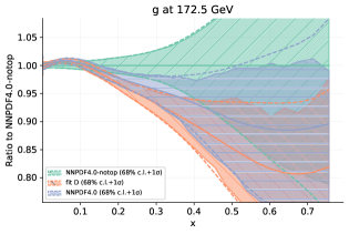
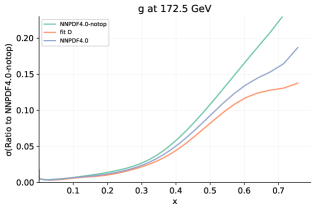
Figure 4.1: Left: comparison between the gluon PDF at $Q=m_{t}=172.5$ GeV obtained in the NNPDF4.0 and NNPDF4.0-notop fits against fit D in Table 4.1, which includes all top-quark pair (also the charge asymmetry $A_{C}$) and single-top quark production data considered in this analysis. Results are normalised to the central value of the NNPDF4.0-notop set. Right: same comparison now for the PDF uncertainties (all normalised to the central value of the NNPDF4.0-notop set).

From Fig. 4.1 one finds that the main impact of the additional LHC Run II $t\bar{t}$ and sinle-top data included in fit D as compared to that already present in NNPDF4.0 is a further depletion of the large-$x$ gluon PDF as compared to the NNPDF4.0-notop baseline, together with a reduction of the PDF uncertainties in the same kinematic region. While fit D and NNPDF4.0 agree within uncertainties in the whole range of $x$, fit D and NNPDF4.0-notop agree only at the $2\sigma$ level in the region $x\approx[0.2,0.4]$. These findings imply that the effect on the SM-PDFs of the new Run II top data is consistent with, and strengthens, that of the data already part of NNPDF4.0 , and suggests a possible tension between top quark data and other measurements in the global PDF sensitive to the large-$x$ gluon, in particular inclusive jet and di-jet production. The reduction of the gluon PDF uncertainties from the new measurements can be as large as about 20% at $x\approx 0.4$. Differences are much reduced for the quark PDFs, and restricted to a 5% to 10% uncertainty reduction in the region around $x\sim 0.2$ with central values essentially unchanged.

To disentangle which of the processes considered dominates the observed effects on the gluon and the light quarks PDFs, Fig. 4.2 compares the relative PDF uncertainty on the gluon and on the $d/u$ quark ratio in the NNPDF4.0-notop baseline fit at $Q=m_{t}=172.5$ GeV with the results from fits A, B, C, and D. As indicated in Table 4.1, these fit variants include the following top datasets: inclusive $t\bar{t}$ (A), inclusive $t\bar{t}$ + $A_{C}$ (B), single top (C), and their sum (D). The inclusion of the top charge asymmetry $A_{C}$ data does not have any impact on the PDFs; indeed fits A and B are statistically equivalent. This is not surprising, given that in Eq. (2.1) the dependence on PDFs cancels out. Concerning the inclusion of single top data (fit C), it does not affect the gluon PDF but instead leads to a moderate reduction on the PDF uncertainties on the light quark PDFs in the intermediate-$x$ region, $x\approx[0.01,0.1]$, as shown in the right panel displaying the relative uncertainty reduction for the $d/u$ ratio. This observation agrees with what was pointed out by a previous study [16], and the impact of LHC single-top measurements is more marked now as expected since the number of data points considered here is larger. We conclude that the inclusive $t\bar{t}$ measurements dominate the impact on the large-$x$ gluon observed in Fig. 4.1, with single top data moderately helping to constrain the light quark PDFs in the intermediate-$x$ region.

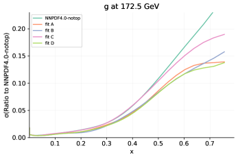
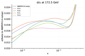
Figure 4.2: The ratio between the PDF 1$\sigma$ uncertainty and the central value of the NNPDF4.0-notop baseline in the case of the gluon (left panel) and in the case of the $d/u$ ratio (right panel). The uncertainty of the baseline fit at $Q=m_{t}=172.5$ GeV is compared with the uncertainty associated with fits A, B, C, and D in Table 4.1. These fit variants include the following top datasets: inclusive $t\bar{t}$ (A), inclusive $t\bar{t}$ + $A_{C}$ (B), single top (C), and their sum (D).

We now consider the effect of the inclusion of data that were not included before in any PDF fit, namely either $t\bar{t}$ or single-top production in association with a weak vector boson. Although current data exhibits large experimental and theoretical uncertainties, it is interesting to study whether they impact PDF fits at all, in view of their increased precision expected in future measurements; in particular, it is useful to know which parton flavours are most affected.

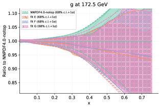
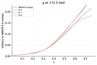
Figure 4.3: Same as Fig. 4.1 comparing the NNPDF4.0-notop baseline fit with variants E, F, and G from Table 4.1. These variants include associated $t\bar{t}$ and vector boson production data (E), associated single top and vector boson production data (F) and their sum (G).

Fig. 4.3 displays the same comparison as in Fig. 4.1 now for the NNPDF4.0-notop baseline and the variants E, F, and G from Table 4.1, which include the $t\bar{t}V$ (E) and $tV$ (F) data as well as their sum (G). The pull of $t\bar{t}V$ is very small, while the pull of the $tV$ measurements is in general small, but consistent with those of the inclusive $t\bar{t}$ measurements, namely preferring a depletion of the large-$x$ gluon. This result indicates that $t\bar{t}V$ and $tV$ data may be helpful in constraining PDF once both future experimental data and theoretical predictions become more precise, although the corresponding inclusive measurements are still expected to provide the dominant constraints.

4.3 Combined effect of the full top quark dataset

The main result of this section is displayed in Fig. 4.4, which compares the NNPDF4.0 and the NNPDF4.0-notop fits with variant H in Table 4.1, namely with the fit where the full set of top quark measurements considered in this analysis has been added to the no-top baseline. As in the case of Fig. 4.1, we show the large-$x$ gluon normalised to the central value of NNPDF4.0-notop and the associated 1$\sigma$ PDF uncertainties (all normalised to the central value of the baseline). The results of fit H are similar to those of fit D, although slightly more marked. This is expected, since as shown above the associated production datasets $t\bar{t}V$ and $tV$ carry little weight in the fit.

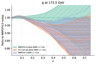
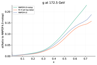
Figure 4.4: Same as Fig. 4.1 comparing NNPDF4.0 and NNPDF4.0 (no top) with fit variant H in Table 4.1, which includes the full set of top quark measurements considered in this analysis.

From Fig. 4.4 one observes how the gluon PDF of fit H deviates from the NNPDF4.0-notop baseline markedly in the data region $x\in[0.1,0.5]$. The shift in the gluon PDF can be up to the $2\sigma$ level, and in particular the two PDF uncertainty bands do not overlap in the region $x\in\left[0.2,0.35\right]$. As before, we observe that the inclusion of the latest Run II top quark measurements enhances the effect of the top data already included in NNPDF4.0 , by further depleting the gluon in the large-$x$ region and by reducing its uncertainty by a factor up to 25%. Hence, one finds again that the new Run II top quark production measurements lead to a strong pull on the large-$x$ gluon, qualitatively consistent but stronger as compared with the pulls associated from the datasets already included in NNPDF4.0 .

To assess the phenomenological impact of our analysis at the level of LHC processes, Fig. 4.5 compares the gluon-gluon and quark-gluon partonic luminosities at $\sqrt{s}=13$ TeV (restricted to the central acceptance region with $|y|\leq 2.5$) between NNPDF4.0 , NNPDF4.0-notop , and fit H including the full top quark dataset considered here and Fig. 4.5 compares their uncertainties. Results are presented as the ratio to the no-top baseline fit. The $qq$ and $q\bar{q}$ luminosities of fit H are essentially identical to those of the no-top baseline, as expected given the negligible changes in the quark PDFs observed in fit H, and hence are not discussed further.

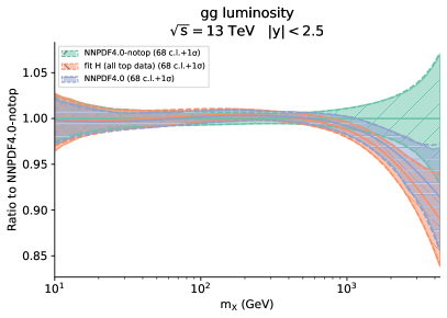
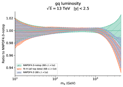
Figure 4.5: The gluon-gluon (left) and quark-gluon (right panel) partonic luminosities at $\sqrt{s}=13$ TeV restricted to the central acceptance region with $|y|\leq 2.5$. We compare the NNPDF4.0 and NNPDF4.0-notop fits with the predictions based on fit H, which includes the full top quark dataset considered here. Results are presented as the ratio to the NNPDF4.0-notop baseline fit.

From Figs. 4.5-4.6 one observes that both for the quark-gluon and gluon-gluon luminosity the impact of the LHC top quark data is concentrated on the region above $m_{X}\mathrel{\hbox to0.0pt{\lower 4.0pt\hbox{\hskip 1.0pt$\sim$}\hss}\raise 1.0pt\hbox{$>$}}1$ TeV. As already reported for the case of the gluon PDF, also for the luminosities the net effect of the new LHC Run II top quark data is to further reduce the luminosities for invariant masses in the TeV range, with a qualitatively similar but stronger pull as compared to that obtained in NNPDF4.0 . While NNPDF4.0 and its no-top variant agree at the $1\sigma$ level in the full kinematical range considered, this is not true for fit H, whose error bands do not overlap with those of NNPDF4.0-notop for invariant masses $m_{X}$ between 2 and 4 TeV. On the other hand, NNPDF4.0 and fit H are fully consistent across the full $m_{X}$ range, and hence we conclude that predictions for LHC observables based on NNPDF4.0 will not be significantly affected by the inclusion of the latest LHC top quark data considered in this work.

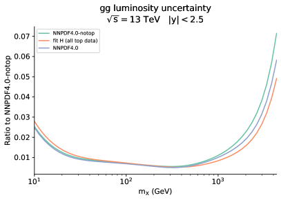
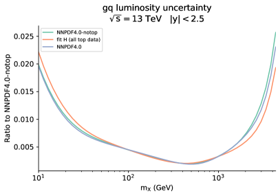
Figure 4.6: Same as Fig. 4.5, now for the relative luminosity uncertainties, all normalised to the NNPDF4.0-notop baseline fit.

Finally, concerning the fit quality of fit H is essentially stable, actually better relative to the NNPDF4.0-notop baseline. The experimental $\chi^{2}$ per data point on their respective datasets is $1.156$ for the no-top baseline, whilst for fit H is reduced to $1.144$. A complete summary of the $\chi^{2}$ information for all of the fits in this section is given in App. D. It is interesting to observe that all new top data included in fit H are already described well by using the NNPDF4.0 set, although clearly the $\chi^{2}$ per data point improves (from $1.139$ to $1.102$) once all data are included in the fit. This confirms the overall consistency of the analysis.

5 Impact of the top quark Run II dataset on the SMEFT

We now quantify the impact of the LHC Run II legacy measurements, described in Sect. 2, on the top quark sector of the SMEFT. As compared to previous investigations of SMEFT operators modifying top-quark interactions [91, 42] [26, 27, 28, 29, 30, 31, 32, 33], the current analysis considers a wider dataset, in particular extended to various measurements based on the full LHC Run II luminosity. In the last column of Tables 2.1–2.8 we indicated which of the datasets included here were considered for the first time within a SMEFT interpretation. Here we assess the constraints that the available LHC top quark measurements provide on the SMEFT parameter space, and in particular study the impact of the new measurements as compared to those used in [91, 42]. In this section we restrict ourselves to fixed-PDF EFT fits, where the input PDFs used in the calculation of the SM cross-sections are kept fixed. Subsequently, in Sect. 6, we generalise to the case in which PDFs are extracted simultaneously together with the EFT coefficients.

The structure of this section is as follows. We begin in Sect. 5.1 by describing the methodologies used to constrain the EFT parameter space both at linear and quadratic order in the EFT expansion. We also present results for the Fisher information matrix, which indicates which datasets provide constraints on which operators. In Sect. 5.2, we proceed to give the results of the fixed-PDF EFT fits at both linear and quadratic order, highlighting the impact of the new Run II top quark data by comparison with previous global SMEFT analyses. In Sect. 5.3, we assess the impact of replacing the CMS 13 TeV differential measurement of $t\bar{t}$ in the $\ell+$jets channel, binned with respect to invariant top quark pair mass, by the corresponding double-differential measurement binned with respect to both invariant top quark pair mass and top quark pair rapidity. In the dataset selection performed in Sect 2.2 we rejected the double-differential distribution due to its poor $\chi^{2}$-statistic in the SM, which could not be improved by a weighted fit of PDFs; in the present section, it is interesting to see whether the SMEFT can help account for the poor fit of this dataset. Finally, in Sect. 5.4 we evaluate the correlation between PDFs and EFT coefficients to identify the kinematic region and EFT operators which are potentially sensitive to the SMEFT-PDF interplay to be studied in Sect. 6.

5.1 Fit settings

Throughout this section, we will allow only the SMEFT coefficients to vary in the fit, keeping the PDFs fixed to the SM-PDFs baseline obtained in the NNPDF4.0-notop fit discussed in Sect. 4; with this choice, one removes the overlap between the datasets entering the PDF fit and the EFT coefficients determination. Our analysis is sensitive to the $N=25$ Wilson coefficients defined in Table B.1, except at the linear level where the four-heavy coefficients $c_{Qt}^{8}$, $c_{QQ}^{1}$, $c_{QQ}^{8}$, $c_{Qt}^{1}$ and $c_{tt}^{1}$ (which are constrained only by $t\bar{t}t\bar{t}$ and $t\bar{t}b\bar{b}$ data) exhibit three flat directions [42]. In order to tackle this, we remove the five four-heavy coefficients from the linear fit Hence, in our linear fit we have $N=20$ independent coefficients constrained from the data, whereas in the quadratic fit, we fit all $N=25$ independent coefficients.

The linear EFT fits presented in this section are performed with the SIMUnet methodology in the fixed-PDF option, as described in Sect. 3; we explicitly verified that the SIMUnet methodology reproduces the posterior distributions provided by SMEFiT (using either the NS (Nested Sampling) or MCfit options) for a common choice of inputs, as explicitly demonstrated in App. C. However, in the case of the quadratic EFT fits we are unable to use the SIMUnet methodology due to a failure of the Monte-Carlo sampling method utilised in the SIMUnet and SMEFiT codes; this is discussed in App. E and a dedicated study of the problem will be the subject of future work. For this reason, quadratic EFT fits in this section are carried out with the public SMEFiT code using the NS mode [171]. To carry out these fits, the full dataset listed in Tables 2.1–2.8, together with the corresponding SM and EFT theory calculations described in Sect. 2.3, have been converted to the SMEFiT data format (this conversion was also already used for the benchmarking of App. C).

Fisher information.

The sensitivity to the EFT operators of the various processes entering the fit can be evaluated by means of the Fisher information, $F_{ij}$, which quantifies the information carried by a given dataset on the EFT coefficients $c_{i}$ [175]. In a linear EFT setting, the Fisher information is given by:

$$F_{ij}=L^{(i)T}({\rm cov}_{\rm exp})^{-1}L^{(j)}$$ (5.1)

where the $k$-th entry, $L^{(i)}_{k}$, of the vector $L^{(i)}$ is the linear contribution multiplying $c_{i}$ in the SMEFT theory prediction for the $k$-th data point, and ${\rm cov}_{\rm exp}$ is the experimental covariance matrix. In particular, the Fisher information is an $N\times N$ matrix, where $N$ is the number of EFT coefficients, and it depends on the dataset. An important property of the Fisher information is that it is related the covariance matrix $C_{ij}$ of the maximum likelihood estimators by the Cramer-Rao bound:

$$C_{ij}\geq(F^{-1})_{ij},$$ (5.2)

indicating that larger values of $F_{ij}$ will translate to tighter bounds on the EFT coefficients.

Before displaying the results of the fixed-PDF SMEFT analysis in Sect. 5.2, we use the Fisher information to assess the relative impact of each sector of top quark data on the EFT parameter space; this is done in the linear analysis, including ${\cal O}(1/\Lambda^{2})$ SMEFT corrections. In the quadratic case, once ${\cal O}(1/\Lambda^{4})$ SMEFT corrections are included, the dependence of $F_{ij}$ on the Wilson coefficients makes interpretation more difficult. Writing $F_{ij}(D)$ for the Fisher information matrix evaluated on the dataset $D$, we define the relative constraining power of the dataset $D$ via:

$$\textrm{relative constraining power of }D\textrm{ on operator }c_{i}=F_{ii}(D)\bigg{/}\displaystyle\sum_{\text{sectors }D^{\prime}}F_{ii}(D^{\prime}).$$ (5.3)

Since $F_{ii}(D)$ corresponds to the constraining power of the dataset $D$ in a one-parameter fit of the Wilson coefficient $c_{i}$, this definition only quantifies how much a dataset impacts one-parameter fits of single Wilson coefficients in turn; however, this will give a general qualitative picture of some of the expected behaviour in the global fit too. We display the results of evaluating the relative constraining power of each top quark data sector on each of the parameters in Fig. 5.1, quoting the results in percent (%).

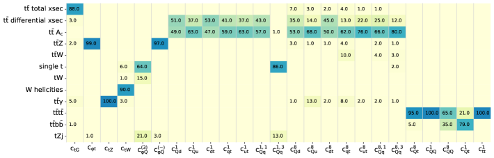
Figure 5.1: Relative constraining power (in %) on each of the operators for each of the processes entering the fit, as defined in Eq. (5.3).

As expected, $t\bar{t}$ total cross sections constitute the dominant source of constraints on the coefficient $c_{tG}$. Each of the four-fermion operators receive important constraints from differential $t\bar{t}$ distributions and charge asymmetry measurements. Note that this impact is magnified when we go beyond individual fits, in which case measurements of charge asymmetries are helpful in breaking flat directions amongst the four-fermion operators [28, 91]. The coefficient $c_{Qq}^{1,3}$ is the exception as it is instead expected to be well-constrained by single top production. We note that the measurements of $W$ helicities are helpful in constraining the coefficient $c_{tW}$, while $t\bar{t}Z$ measurements provide the dominant source of constraints on $c_{\varphi Q}^{(-)}$. We observe that the neutral top coupling $c_{tZ}$ is entirely constrained by $t\bar{t}\gamma$, and that the effects of $t\bar{t}t\bar{t}$ and $t\bar{t}b\bar{b}$ are mostly restricted to the 4-heavy operators $c_{Qt}^{8}$, $c_{QQ}^{1}$, $c_{QQ}^{8}$, $c_{Qt}^{1}$ and $c_{tt}^{1}$.

5.2 Fixed-PDF EFT fit results

In this section, we present the results of the linear and quadratic fixed-PDF fits with the settings described in Sect 5.1.

Fit quality.

We begin by discussing the fit quality of the global SMEFT determination, quantifying the change in the data-theory agreement relative to the SM in both the linear and quadratic SMEFT scenarios. Table 5.1 provides the values of the $\chi^{2}$ per data point in the SM and in the case of the SMEFT at both linear and quadratic order in the EFT expansion for each of the processes entering the fit. Here, in order to ease the comparison of our results to those of SMEFiT and FitMaker, we quote the $\chi^{2}$ per data point computed by using the covariance matrix defined in Eq. (3.7), which includes both the experimental uncertainty and the PDF uncertainty. The corresponding values obtained by using the experimental $\chi^{2}$ definition of Eq. (2.3), along with a fine-grained fit quality description are given in App. D.

We observe that in many sectors, the linear EFT fit improves the fit quality compared to the SM; notably, the $\chi^{2}_{\rm exp+th}$ per data point for inclusive $t\bar{t}$ is vastly improved from 1.71 to 1.11. When quadratic corrections are also considered, the fit quality is usually poorer compared to the linear fit. For example, in inclusive $t\bar{t}$ the $\chi^{2}_{\rm exp+th}$ per data point deteriorates from 1.11 to 1.69. This is not unexpected, however, since the flexibility of the quadratic fit is limited by the fact that for sufficiently large values of Wilson coefficients the EFT can only make positive corrections.

Process	$n_{\rm dat}$	$\chi^{2}_{\rm exp+th}$ [SM]	$\chi^{2}_{\rm exp+th}$ [SMEFT $\mathcal{O}(\Lambda^{-2})]$	$\chi^{2}_{\rm exp+th}$ [SMEFT $\mathcal{O}(\Lambda^{-4})]$
$t\bar{t}$	86	1.71	1.11	1.69
$t\bar{t}$ AC	18	0.58	0.50	0.60
$W$ helicities	4	0.71	0.45	0.47
$t\bar{t}Z$	12	1.19	1.17	0.94
$t\bar{t}W$	4	1.71	0.46	1.66
$t\bar{t}\gamma$	2	0.47	0.03	0.59
$t\bar{t}t\bar{t}$ & $t\bar{t}b\bar{b}$	8	1.32	1.06	0.49
single top	30	0.504	0.33	0.37
$tW$	6	1.00	0.82	0.82
$tZ$	5	0.45	0.30	0.31
Total	175	1.24	0.84	1.14

Table 5.1: The values of the $\chi^{2}$ per data point for the fixed-PDF EFT fits presented in this section, both for individual groups of processes, and for the total dataset. Here the $\chi^{2}$ is actually the $\chi^{2}_{\rm exp+th}$ defined by using the theory covariance matrix defined in Eq. (3.7). In each case we indicate the number of data points, the $\chi^{2}_{\rm exp+th}$ obtained using the baseline SM calculations, and the results of both the linear and quadratic EFT fits.

It is also useful to calculate the goodness of fit, quantified by the the $\chi^{2}$ per degree of freedom, $\chi^{2}/n_{\rm dof}=\chi^{2}/(n_{\rm dat}-n_{\rm param})$, which additionally accounts for the complexity of the models we are using in each fit. In our case, we find $\chi^{2}_{\rm exp+th}/n_{\rm dof}=1.25$ in the SM and $\chi^{2}_{\rm exp+th}/n_{\rm dof}=0.95$ and $1.33$ in the linear and quadratic EFT scenarios respectively. We see that while the EFT at quadratic order does not provide a better fit than the SM, neglecting quadratic EFT corrections leads to a significant improvement in the overall fit quality.

Constraints on the EFT parameter space.

Next, we present the constraints on the EFT parameter space. In Fig. 5.2, we display the 95% CL constraints on the 20 Wilson coefficients entering the linear fit. Two sets of constraints are shown; in green, we give the intervals obtained from a fit to the 175 data points introduced in Sect. 2, whilst in orange, we give in the intervals obtained from a fit to the older top quark dataset used in the global analysis of Ref. [42], obtained from a fit of 150 data points. This comparison allows us to quantify the information gained from the latest Run II datasets, relative to those available to previous analyses. The same comparison, this time at quadratic order in the EFT expansion, is shown in Fig. 5.3 (note that in this plot we display constraints on all 25 coefficients, including the 4-heavy coefficients $c_{Qt}^{8}$, $c_{QQ}^{1}$, $c_{QQ}^{8}$, $c_{Qt}^{1}$ and $c_{tt}^{1}$).

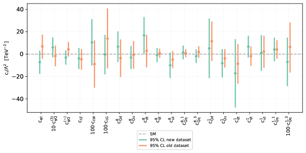
Figure 5.2: The 95% CL intervals on the EFT coefficients entering the linear fit, evaluated with SIMUnet on the dataset considered in this work, and evaluated with SMEFiT on the top quark dataset entering the analysis of [42] (note that at the linear EFT level, the results obtained with SIMUnet coincide with those provided by SMEFiT for the same dataset, as demonstrated in App. C). Note also that the constraints on selected coefficients are rescaled by the factors shown, for display purposes.

We first note that Figures 5.2 and 5.3 both demonstrate good agreement between the fits using old and new datasets, and consistency between the new fit SMEFT bounds and the SM. At the linear level, the most noticeable improvement concerns $c_{tG}$; its 95% C.L. bounds decrease from $[-0.13,0.41]$ to $[-0.18,0.17]$, thanks to the increased amount of information in the input dataset, coming in particular from $t\bar{t}$ data. This results in both a tightening of the constraints by about 35% and a shift in the best-fit point. For many of the other coefficients, the bounds are either stable (e.g. $c_{tZ}$), or exhibit a shift in central value but no significant tightening (e.g. $c_{\varphi t}$, undergoes a shift of -14.3, but a decrease in the size of the constraints 95% C.L. by only 1%, and $c_{\varphi Q}^{(-)}$ undergoes a shift of $-7.33$, but its bounds only tighten by 2%). Finally, we note that some coefficients instead exhibit a broadening of constraints with the new dataset relative to the old dataset (for example, some of the four-fermion operators). The increase in the size of the constraints could point to some inconsistency within the new inclusive $t\bar{t}$ dataset; however, given that the bounds are very large anyway, at the edges of the intervals we are likely to approach a region where the EFT is no longer valid in both cases, hence no definite conclusions may be drawn.

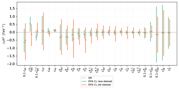
Figure 5.3: The 95% CL intervals on the EFT coefficients entering the quadratic fit, evaluated with SMEFiT. We compare the results based on the full top quark dataset with the corresponding results obtained from the subset of top quark measurements entering the analysis of [42]. As in Fig. 5.2, the constraints on selected coefficients are rescaled by the factors shown, for display purposes.

At the quadratic order in the EFT expansion, however, the impact of the latest Run II dataset is clear; we see a marked improvement in many of the SMEFT constraints. As shown in Fig. 5.3, the bounds on all 14 of the four-fermion operators become noticeably smaller as a result of the increase in precision in the $t\bar{t}$ sector. The constraint on $c_{tZ}$ is improved by the inclusion of measurements of the $t\bar{t}\gamma$ total cross sections, resulting in a tightening of 24%. The addition of the $p_{T}^{\gamma}$ spectrum [129] would yield an even stronger constraint, as seen in [91]. We will make use of this observable in future work when unfolded measurements are made available. Contrary to the linear fit, where we singled out $c_{\varphi t}$ and $c_{\varphi Q}^{(-)}$ as examples of coefficients which shift, but whose bounds are not improved, the constraints on $c_{\varphi t}$, $c_{\varphi Q}^{(-)}$ markedly tighten in the quadratic fit in the presence of new data; in particular, the size of the bounds on $c_{\varphi t}$, $c_{\varphi Q}^{(-)}$ decrease by 35% and 28%, respectively. On the other hand, despite the addition of new $t\bar{t}t\bar{t}$, $t\bar{t}b\bar{b}$ datasets, we find limited sensitivity to the five four-heavy coefficients $c_{Qt}^{8}$, $c_{QQ}^{1}$, $c_{QQ}^{8}$, $c_{Qt}^{1}$ and $c_{tt}^{1}$. In fact, with the new data we see a broadening of the bounds. As with the linear fit, this could point to either an inconsistency in the $t\bar{t}t\bar{t}$, $t\bar{t}b\bar{b}$ data, or simply to the ambiguity associated to the EFT validity in that particular region of the parameter space.

Correlations.

Figure 5.4 shows the correlations the between Wilson coefficients evaluated in this analysis both at the linear and the quadratic order in the EFT expansion, shown on the left and right panels respectively. In the linear fit, we first note a number of large correlations amongst the octet four-fermion operators which enter the $t\bar{t}$ production together. The singlet four-fermion operators are similarly correlated among themselves, although their correlations are comparatively suppressed. The coefficients $c_{\varphi t}$ and $c_{\varphi Q}^{(-)}$ exhibit a large positive correlation due to their entering into $t\bar{t}Z$ production together, while $c_{Qq}^{3,1}$ and $c_{\varphi Q}^{(3)}$ have positive correlations through their contribution to single top production. Further non-zero correlations are found, for example amongst the pairs $c_{Qq}^{8,3}$ & $c_{\varphi Q}^{(3)}$, $c_{Qd}^{8}$ & $c_{tZ}$ and $c_{Qu}^{8}$ & $c_{tZ}$.

At quadratic order, however, we observe that many of these correlations are suppressed, as a result of the fact that the inclusion of quadratic corrections lifts many of the degeneracies in the fit. We observe that the pairs $c_{\varphi t}$, $c_{\varphi Q}^{(-)}$ and $c_{Qq}^{1,3}$, $c_{\varphi Q}^{(3)}$ remain correlated though. The 4-heavy operators are also included in this quadratic fit, and we find large anti-correlations between $c_{QQ}^{1}$ and $c_{QQ}^{8}$, indicating that they are poorly distinguished in the $t\bar{t}t\bar{t}$ and $t\bar{t}b\bar{b}$ processes. Finally, note that we obtain subtle non-zero correlations between the octet and singlet four-fermion operators constructed from the same fields, for example between $c_{Qd}^{8}$ and $c_{Qd}^{1}$. This is a result of the fact that $t\bar{t}$ measurements provide the dominant source of constraints on these coefficients and are very sensitive to quadratic corrections, and at this order the contribution from these operators differs only by a numerical factor.

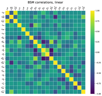
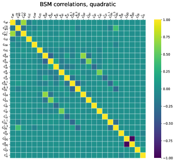
Figure 5.4: The values of the correlation coefficients evaluated between all pairs of Wilson coefficients entering the EFT fit at the linear (left) and quadratic (right) order. As explained in the next, the number of fitted DoFs is different in each case.

5.3 Study of the CMS 1D vs 2D distribution

In the dataset selection discussed in Sect. 2.2, the double-differential distribution measurements performed by CMS at $\sqrt{s}=13$ TeV in the $\ell+$jets channel [106] – binned with respect to the top quark pair invariant mass $m_{t\bar{t}}$ and the top quark pair rapidity $y_{t\bar{t}}$ – is found to be poorly described by the SM theory, with an experimental $\chi^{2}$ that is $22\sigma$ away from the median of the $\chi^{2}$ distribution of a perfectly consistent dataset made of $n_{\rm dat}=34$. Even by increasing the weight of this dataset in a weighted fit (see Sect. 2.2 for a more detailed explanation), the $\chi^{2}_{\rm exp}$ per data point improves only moderately to 4.56 and the $\chi^{2}$-statistic of the other datasets deteriorates significantly, hinting to both an internal incompatibility of the CMS 2D distribution and to an incompatibility with the rest of the data. For this reason, the dataset was excluded from our analysis, and replaced by the the single-differential distribution in $m_{t\bar{t}}$ – presented in the same publication [106]. The latter is well described by the SM theoretical predictions.

In this section we present a dedicated analysis to assess whether the SMEFT corrections can improve the theoretical description of this dataset. In particular, we compare a fixed-PDF fit including the 13 TeV CMS double-differential $(m_{t\bar{t}},y_{t\bar{t}})$ distribution (CMS 2D) to the default one including the 13 TeV single-differential $m_{t\bar{t}}$ distribution (CMS 1D).

Process	$\qquad n_{\rm dat}\qquad$	$\chi^{2}_{\rm exp+th}$ [SM]		$\chi^{2}_{\rm exp+th}$ [SMEFT $\mathcal{O}(\Lambda^{-2})]$		$\chi^{2}_{\rm exp+th}$ [SMEFT $\mathcal{O}(\Lambda^{-4})]$
		CMS 1D	CMS 2D	CMS 1D	CMS 2D	CMS 1D	CMS 2D
$t\bar{t}$	86	1.71	2.07	1.11	1.18	1.69	1.87
$t\bar{t}$ AC	18	0.58	0.58	0.50	0.47	0.60	0.60
$W$ helicities	4	0.71	0.71	0.45	0.45	0.48	0.46
$t\bar{t}Z$	12	1.19	1.19	1.17	1.07	0.94	0.95
$t\bar{t}W$	4	1.71	1.71	0.46	0.46	1.66	1.82
$t\bar{t}\gamma$	2	0.47	0.47	0.03	0.03	0.58	0.18
$t\bar{t}t\bar{t}$ & $t\bar{t}b\bar{b}$	8	1.32	1.32	1.06	1.28	0.49	0.49
single top	30	0.50	0.50	0.33	0.34	0.37	0.35
$tW$	6	1.00	01.00	0.82	0.86	0.82	0.84
$tZ$	5	0.45	0.45	0.30	0.30	0.31	0.30
Total	175	1.24	1.48	0.84	0.91	1.14	1.29

Table 5.2: Same as Table 5.1, now comparing the values of the $\chi^{2}_{\rm exp+th}$ per data point for the fixed-PDF EFT fits presented in this section, the default one including the 13 TeV single-differential $m_{t\bar{t}}$ distribution (CMS 1D) and the one including the 13 TeV CMS double-differential $(m_{t\bar{t}},y_{t\bar{t}})$ distribution (CMS 2D), both for individual groups of processes, and for the total dataset.

First of all, it is interesting to notice that the inclusion of quadratic SMEFT corrections in the fit does not improve much the quality of the fit of the CMS 2D distribution, with $\chi^{2}_{\rm exp+th}/n_{\rm dat}$ decreasing from 2.80 (in the SM) to $\chi^{2}_{\rm exp+th}/n_{\rm dat}=2.57$ including SMEFT $\mathcal{O}(\Lambda^{-4})$ corrections. On the other hand, if SMEFT linear $\mathcal{O}(\Lambda^{-2})$ corrections are included, the fit quality of the CMS 2D distribution improves substantially with $\chi^{2}_{\rm exp+th}/n_{\rm dat}=1.22$.

In order to assess what is the effect of the inclusion of the CMS 2D distribution on the other top sector data, in Table 5.2 we compare the fit quality of the two (fixed-PDF) SMEFT fits, CMS 1D and CMS 2D, both for individual groups of processes, and for the total dataset. We observe that the fit quality deteriorates both in the SM and in the quadratic SMEFT fit once the CMS 2D distribution is fitted. The deterioration of the fit quality is mostly driven by a deterioration of the fit quality of the $t\bar{t}$ and $t\bar{t}W$ sectors. However at the level of linear SMEFT fit, the quality of the fit deteriorates only moderately and it is mostly driven by the slight deterioration in the inclusive $t\bar{t}$ sector and in the $t\bar{t}t\bar{t}\,\&\,t\bar{t}b\bar{b}$ one.

At the level of fit of the Wilson coefficients, the quadratic SMEFT fits yields similar 95% C.L. bounds on the EFT coefficients. This is somewhat expected, given that the fit quality of the CMS 2D data does not improve once quadratic SMEFT corrections are included, and the fit quality of the other datasets remains pretty much the same.

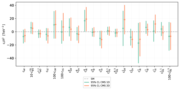
Figure 5.5: The 95% CL intervals on the EFT coefficients entering the liner fits, evaluated with SIMUnet. We compare the results based on the default full top quark dataset (CMS 1D) with the corresponding results obtained from the same set of top quark measurements in which the single-differential $m_{t\bar{t}}$ 13 TeV CMS distribution is substituted by the double differential $(m_{t\bar{t}},y_{t\bar{t}})$ 13 TeV CMS distribution (CMS 2D).

On the other hand the bounds obtained from a SMEFT linear fit change more significantly depending on whether the CMS 1D or the CMS 2D distribution is used in the fit. In particular the central value of the $c_{tG}$ 95% C.L. bounds is shifted upwards by 1$\sigma$, as well as the bounds on $c^{1}_{Qd}$ and $c^{1}_{ut}$, while the bounds on $c^{1}_{Qu}$ and $c^{1}_{qt}$ shift downwards, as expected from the EFT coefficient correlations displayed in Fig. 5.4.

As a result of our analysis, we observe that the bounds on the EFT in the linear case do depend on the input dataset quite significantly and careful consideration has to be made to the overall dataset compatibility and to the outcome of the fit once quadratic corrections are included. The current analysis in particular shows that the incompatibility of the 13 TeV CMS double differential distribution cannot be entirely attributed to new physics effects parametrised by the SMEFT expansion, rather there are internal experimental or theoretical incompatibilities that affect the results.

5.4 Correlations between PDFs and EFT coefficients

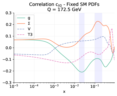
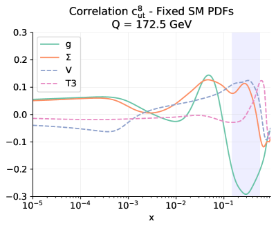
Figure 5.6: The value of the correlation coefficient $\rho$ between the PDFs and selected EFT coefficients as a function of $x$ and $Q=172.5$ GeV. We show the results for the gluon, the total singlet $\Sigma$, total valence $V$, and non-singlet triplet $T_{3}$ PDFs. We provide results for representative EFT coefficients, namely $c_{tG}$ and $c_{ut}^{(8)}$.

We conclude this section by discussing the correlations observed between the PDFs and Wilson coefficients. The PDF-EFT correlation coefficient for a Wilson coefficient $c$ and a PDF $f(x,Q)$ at a given $x$ and $Q^{2}$ is defined as

$$\rho\left(c,f(x,Q^{2})\right)={{\left\langle c^{(k)}f^{(k)}(x,Q^{2})\right\rangle_{k}-\left\langle c^{(k)}\right\rangle_{k}\left\langle f^{(k)}(x,Q^{2})\right\rangle_{k}}\over{\sqrt{\left\langle(c^{(k)})^{2}\right\rangle_{k}-\left\langle c^{(k)}\right\rangle_{k}^{2}}\sqrt{\left\langle\left(f^{(k)}(x,Q^{2})\right)^{2}\right\rangle_{k}-\left\langle f^{(k)}(x,Q^{2})\right\rangle_{k}^{2}}}}\,,$$ (5.4)

where $c^{(k))}$ is the best-fit value of the Wilson coefficient for the $k$-th replica and $f^{(k)}$ is the $k$-th PDF replica computed at a given $x$ and $Q$, and $\left\langle\cdot\right\rangle_{k}$ represents the average over all replicas. We will compute the correlation between a SM PDF and the Wilson coefficients, both of which have been separately determined from the total dataset including all new top quark data. By doing so we hope to shed light on which Wilson coefficients, and which PDF flavours and kinematical regions, are strongly impacted by the top quark data and therefore exhibit a potential for interplay in a simultaneous EFT-PDF determination. The EFT corrections will be restricted to linear order in the EFT expansion.

Fig. 5.6 displays a selection of the largest correlations. We observe that the gluon PDF in the large-$x$ region is significantly correlated with the Wilson coefficients $c_{tG}$, $c_{ut}^{(8)}$. On the other hand, relatively large correlations are observed between $c_{tG}$ and the the total singlet $\Sigma$, while the total valence $V$, and non-singlet triplet $T_{3}$ PDFs show no relevant correlations with the selected coefficients. This is not surprising, given the impact of top quark pair production total cross sections and differential distributions in constraining these PDFs and Wilson coefficients. Whilst these correlations are computed from a determination of the SMEFT in which the PDFs are fixed to SM PDFs, the emergence of non-zero correlations provides an indication of the potential for interplay between the PDFs and the SMEFT coefficients; this interplay will be investigated in a simultaneous determination in the following section.

6 SMEFT-PDFs from top quark data

In this section we present the main results of this work, namely the simultaneous determination of the proton PDFs and the SMEFT Wilson coefficients from the LHC Run II top quark data described in Sect. 2, following the SIMUnet methodology summarised in Sect. 3. This determination of the SMEFT-PDFs from top quark data is carried out at the linear, $\mathcal{O}(1/\Lambda^{2})$, level in the EFT expansion. We do not perform simultaneous fits at the quadratic level due to shortcomings of the Monte Carlo replica method, on which SIMUnet is based; this is discussed in detail in App. E, and will also be the subject of future work.

PDFs from a joint SMEFT-PDF fit.

We begin by discussing the PDFs obtained through a joint fit of PDFs and Wilson coefficients from the complete LHC top quark dataset considered in this work. Simultaneously extracting the PDFs and the EFT coefficients from top quark data has a marked impact on the former, as compared to a SM-PDF baseline, but we shall see has much less impact on the latter, as compared to the results of the corresponding fixed-PDF EFT analyses. Fig. 6.1 displays a comparison between the gluon and quark singlet PDFs, as well as of their relative $1\sigma$ PDF uncertainties, for the NNPDF4.0-notop baseline, the SM-PDFs of fit H in Table 4.1 which include the full top quark dataset, and their SMEFT-PDF counterparts based on the same dataset. PDFs are compared in the large-$x$ region for $Q=m_{t}=172.5$ GeV. In the left panel they are normalised to the central value of the NNPDF4.0-notop fit.

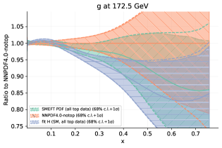
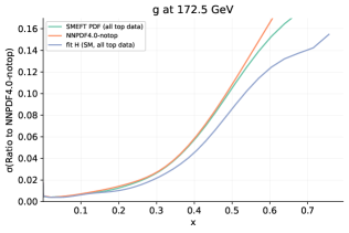
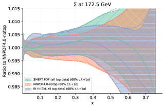
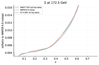
Figure 6.1: Left: a comparison between the gluon (upper panel) and quark singlet (lower panel) PDFs evaluated at $Q=m_{t}=172.5$ GeV in the large-$x$ region. We display the NNPDF4.0-notop baseline, the SM-PDFs of fit H in Table 4.1 which include the full top quark dataset, and their SMEFT-PDF counterparts. The results are normalised to the central value of the NNPDF4.0-notop fit. Right: the same comparison, but now for the relative $1\sigma$ PDF uncertainties.

While differences are negligible for the quark singlet PDF, both in terms of central values and uncertainties, they are more marked for the gluon PDF. Two main effects are observed therein. First, the central value of the SMEFT-PDF gluon moves upwards as compared to the SM-PDF fit based on the same dataset, ending up halfway between the latter and the NNPDF4.0-notop fit. Second, uncertainties increase for the SMEFT-PDF determination as compared to the SM-PDFs extracted from the same data, becoming close to the uncertainties of the NNPDF4.0-notop fit except for $x\mathrel{\hbox to0.0pt{\lower 4.0pt\hbox{\hskip 1.0pt$\sim$}\hss}\raise 1.0pt\hbox{$>$}}0.5$. In both cases, differences are restricted to the large-$x$ region with $x\mathrel{\hbox to0.0pt{\lower 4.0pt\hbox{\hskip 1.0pt$\sim$}\hss}\raise 1.0pt\hbox{$>$}}0.1$, where the impact of the dominant top quark pair production measurements is the largest.

The results of Fig. 6.1 for the gluon PDF therefore indicate that within a simultaneous extraction of the PDFs and the EFT coefficients, the impact of the top quark data on the PDFs is diluted, with the constraints it provides partially ‘reabsorbed’ by the Wilson coefficients. This said, there remains a pull of the top quark data as compared to the no-top baseline fit which is qualitatively consistent with the pull obtained in a SM-PDF determination based on the same dataset, albeit of reduced magnitude. Interestingly, as we show below, while the SMEFT-PDF gluon is significantly modified in the joint fit as compared to a SM-PDF reference, much smaller differences are observed at the level of the bounds on the EFT parameters themselves.

Fig. 6.2 displays the same comparison as in Fig. 6.1 now for the case of the gluon-gluon and quark-gluon partonic luminosities at $\sqrt{s}=13$ TeV, as a function of the final-state invariant mass $m_{X}$. Consistently with the results obtained at the PDF level, one finds that the three luminosities are almost identical for $m_{X}\leq 1$ TeV, and at higher invariant masses the SMEFT-PDF predictions are bracketed between the NNPDF4.0-notop fit from above and the SM-PDF which includes all top data (fit H in Table 4.1) from below. Hence, the net effect of simultaneously fitting the PDFs and the EFT coefficients is a dilution of constraints provided by the top quark data on the former, which translates into larger PDF uncertainties (which end up being rather similar to those of NNPDF4.0-notop ) and an increase in the large-$m_{X}$ luminosity, e.g. of 5% in the $gg$ case for $m_{X}\simeq 3$ TeV, as compared to the SM-PDF luminosity.

This dilution arises because of an improved description of the top quark data included in the fit, especially in the high $m_{t\bar{t}}$ bins. In the SM-PDF case this can only be obtained by suppressing the large-$x$ gluon, while in a SMEFT-PDF analysis this can also be achieved by shifting the EFT coefficients from their SM values. In other words, as compared to the NNPDF4.0-notop baseline, the gluon PDF experiences a suppression at large-$x$ of up to 10% when fitting the top quark data, and this pull is reduced by approximately a factor two in the joint SMEFT-PDF determination due to the coherent effect of the linear EFT cross-sections.

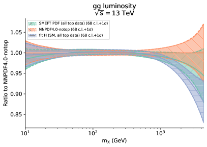
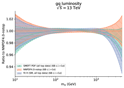
Figure 6.2: The gluon-gluon (left panel) and quark-gluon (right panel) partonic luminosities at $\sqrt{s}=13$ TeV as a function of the final-state invariant mass $m_{X}$. We compare theNNPDF4.0-notop baseline fit with its SM-PDF counterpart including all top quark data considered (fit H in Table 4.1) as well as with the SMEFT-PDF determination. Results are presented as the ratio to the central value of the NNPDF4.0-notop baseline.

EFT coefficients from a joint SMEFT-PDF fit.

As opposed to the marked effect of the SMEFT-PDF interplay found for the large-$x$ gluon, its impact is more moderate at the level of the bounds on the EFT coefficients, and is restricted to mild shifts in the central values and a slight broadening of the uncertainties. This is illustrated by Fig. 6.3, showing the posterior distributions for the Wilson coefficient $c_{tG}$ associated to the chromomagnetic operator in the joint SMEFT-PDF determination, compared with the corresponding results from the fixed-PDF EFT analysis whose settings are described in Sect. 5. The comparison is presented both for the fits which consider only top-quark pair production data and those based on the whole top quark dataset considered in this work. The leading effect of the chromomagnetic operator $\mathcal{O}_{tG}$ is to modify the total rates of $t\bar{t}$ production without altering the shape of the differential distributions, and hence it plays an important role in a simultaneous SMEFT-PDF determination based on top quark data.

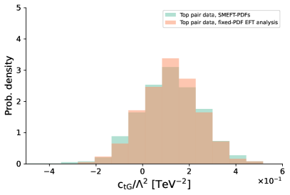
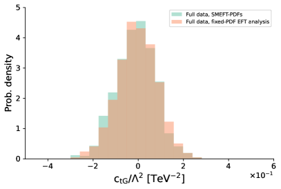
Figure 6.3: Posterior distributions for the Wilson coefficient $c_{tG}$ associated to the chromomagnetic operator in the joint SMEFT-PDF determination, compared with the corresponding results from the fixed-PDF EFT analysis whose settings are described in Sect. 5. We show results based on only top-quark pair production data (left) and in the whole top quark dataset considered in this work (right panel).

For fits based only on inclusive $t\bar{t}$ data, as shown in the left panel of Fig. 6.3, the two posterior distributions are similar; the distribution based on the SMEFT-PDF analysis is slightly broader, approximately $10\%$ so, as compared to the fixed-PDF EFT fit to the same measurements. This slight broadening is washed out in the fit to the full top quark dataset, as shown in the right panel of Fig. 6.3. In both cases, the determination of $c_{tG}$ is consistent with the SM at a 95% CL, and the best-fit values of the coefficient are the same in the SMEFT-PDF and fixed-PDF EFT analyses. Hence, in the specific case of the chromomagnetic operator, the interplay between PDFs and EFT fits is rather moderate and restricted to a broadening of at most $10\%$ in the 95% CL bounds. Similar comparisons have been carried out for other EFT coefficients as well as in the context of fits to a subset of the data and/or to a subset of the coefficients. We find that in general the impact of the SMEFT-PDF interplay translates to a broadening of the uncertainties in the EFT coefficients, which at most reaches $30\%$, and alongside which the best-fit values remain stable.

All in all, within the global fit based on the best available theory predictions, results for the EFT coefficients turn out to be very similar in the fixed-PDF EFT and SMEFT-PDF fits. This indicates that, provided a broad enough dataset and the most up-to-date theory calculations are used, the PDF dependence on the cross-sections entering an EFT interpretation of the LHC data is currently subdominant and can be neglected (this is not the case for the PDFs, see Fig. 6.2). Nevertheless, this statement applies only to the dataset currently available, and it is likely that the SMEFT-PDF interplay will become more significant in the future once HL-LHC measurements become available [176, 177], as demonstrated in the case of high-mass Drell-Yan [35].

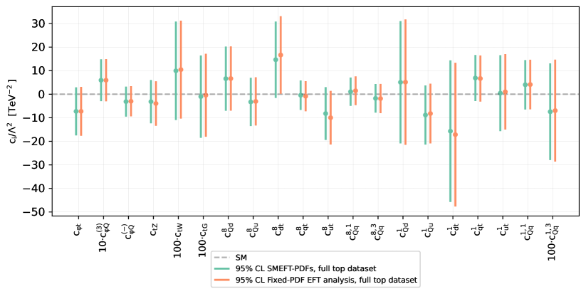
Figure 6.4: Comparison of the $95\%$ CL intervals on the 20 Wilson coefficients considered in this work (in the linear EFT case) between the outcome of the joint SMEFT-PDF determination and that of the fixed-PDF EFT analysis. The latter is based on SM and EFT calculations performed with NNPDF4.0-notop as input, see also Sect. 5. In both cases, results are based on the full top quark dataset being considered and EFT cross-sections are evaluated up to linear, $\mathcal{O}\left(\Lambda^{-2}\right)$, corrections. The dashed horizontal line indicates the SM prediction, $c_{k}=0$. Note that some coefficients are multiplied by the indicated prefactor to facilitate the visualisation of the results.

The moderate impact of the SMEFT-PDF interplay on the Wilson coefficients for the full top quark dataset considered in this work is summarised in Fig. 6.4, which compares the $95\%$ CL intervals of the 20 fitted Wilson coefficients relevant for the linear EFT fit obtained from the outcome of the joint SMEFT-PDF determination and the fixed-PDF EFT analysis. The latter is based on SM and EFT calculations performed with NNPDF4.0-notop as input; see also the description of the settings in Sect. 5. The dashed horizontal line indicates the SM prediction, and some coefficients are multiplied by the indicated prefactor to facilitate the visualisation of the results. Fig. 6.4 demonstrates that, other than slight broadenings and shifts in the central values, the results of the two analyses coincide.

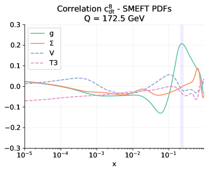
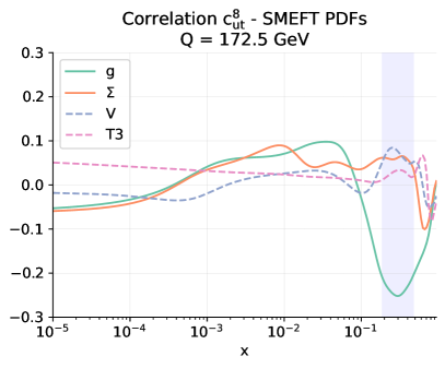
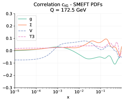
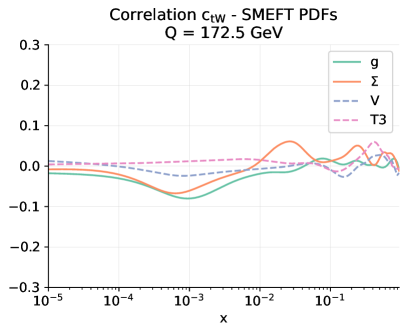
Figure 6.5: The correlation coefficient $\rho(f_{i},c_{k})$ between the SMEFT-PDFs $f_{i}$ and the Wilson coefficients $c_{k}$ evaluated at $Q=172.5$ GeV as a function of $x$. Each panel displays the correlations of the coefficient $c_{k}$ with the gluon and the total singlet $\Sigma$, total valence $V$, and non-singlet triplet $T_{3}$ PDFs. We provide results for representative EFT coefficients, namely $c_{td}^{8}$, $c_{tu}^{8}$, $c_{tG}$, and $c_{tW}$. The largest correlations within the EFT coefficients considered in this work are associated to four-fermion operators such as $c_{td}^{8}$ and $c_{tu}^{8}$.

Correlations.

Fig. 6.5 displays the correlation coefficients [166] between the SMEFT-PDFs and the Wilson coefficients evaluated at $Q=172.5$ GeV as a function of $x$. Each panel displays the correlations of the coefficient $c_{k}$ with the gluon and the total singlet $\Sigma$, total valence $V$, and non-singlet triplet $T_{3}$ PDFs, and we consider four representative EFT coefficients, namely $c_{td}^{8}$, $c_{tu}^{8}$, $c_{tG}$, and $c_{tW}$. The largest correlations within the EFT coefficients considered in this work are associated to the gluon PDF and four-fermion operators such as $c_{td}^{8}$ and $c_{tu}^{8}$ in the large-$x$ region, peaking at $x\simeq 0.3$. Correlations for other values of $x$ and for the quark PDFs are negligible for all operators entering the analysis. We note that future data with an enhanced coverage of the high-$m_{t\bar{t}}$ region in top quark pair-production might alter this picture, given that for $m_{t\bar{t}}\mathrel{\hbox to0.0pt{\lower 4.0pt\hbox{\hskip 1.0pt$\sim$}\hss}\raise 1.0pt\hbox{$>$}}3$ TeV the $q\bar{q}$ luminosity starts to become more relevant and eventually dominates over the $gg$ contribution.

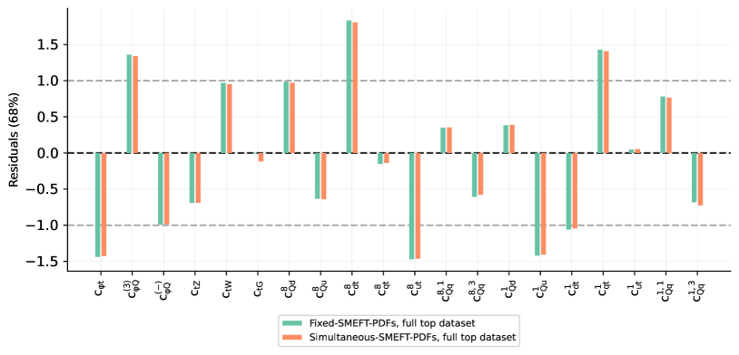
Figure 6.6: The 68% CL residuals, Eq. (6.1), for the same Wilson coefficients displayed in Fig. 6.4, comparing the outcome of the joint SMEFT-PDF determination with that of a fixed-PDF EFT analysis. In the latter, we use as input for the theory calculations the SMEFT-PDFs obtained in the joint fit rather than the NNPDF4.0-notop set used in Sect. 5. The horizontal dashed lines indicate the $\pm 1\sigma$ regions.

Residuals.

Finally, Fig. 6.6 displays a similar comparison as in Fig. 6.4 now at the level of the 68% CL fit residuals defined as

$$R_{n}={{c_{n}^{*}}\over{\sigma_{n}}}\,,$$ (6.1)

where $c_{n}^{*}$ and $\sigma_{n}$ are the median value and the standard deviation of the Wilson coefficient $c_{n}$ respectively, with $n=1,\ldots,N$, where $N$ is the number of operators. The outcome of the joint SMEFT-PDF determination is compared with that of a fixed-PDF EFT analysis where we use as input for the theory calculations the SMEFT-PDFs obtained in the joint fit, rather than the NNPDF4.0-notop set. That is, in both cases the information provided by the top quark data on the PDFs and Wilson coefficients is accounted for, but in one case the cross-correlations are neglected whereas they are accounted for in the other. The residuals are similar in the two cases; they are slightly bigger (in absolute value) in the fixed-PDF case in which the correlations between the SMEFT-PDFs and the EFT coefficients are ignored. This analysis further emphasises that, for the currently available top quark data, the cross-talk between PDFs and EFT degrees of freedom does not significantly modify the posterior distributions in the space spanned by the Wilson coefficients.

In summary, on the one hand we find that from the point of view of a PDF determination, SM-PDFs and SMEFT-PDFs extracted from top quark data differ by an amount comparable to their respective uncertainties in the case of the large-$x$ gluon. On the other hand, at the level of Wilson coefficients the results are unchanged irrespective of the PDF set used as input for the theory calculations; that is, bounds based on NNPDF4.0-notop or the SMEFT-PDFs are almost the same. Hence, while EFT interpretations of top quark data can safely ignore the PDF dependence, at least for the settings adopted in this work, a global PDF fit could be significantly distorted if BSM physics were to be present in the large-energy top quark distributions. We use these findings in App. A to provide recommendations for interpretations of LHC top quark data in the context of either PDF or EFT analyses.

7 Conclusions and outlook

In this work we have carried out a comprehensive theoretical interpretation of top quark data from the LHC, including all available measurements based on the full integrated luminosity of Run II, in terms of the proton PDFs and of Wilson coefficients in the SMEFT. We have integrated a global determination of PDFs with the fit of dimension-six Wilson coefficients modifying top quark interactions into a simultaneous determination of the SMEFT-PDFs and the EFT coefficients. The main outcome of our analysis is the assessment of the conditions under which the usual assumptions of SM-PDFs and fixed-PDF EFT analyses are valid, and establishing when the SMEFT-PDF interplay cannot be neglected without introducing a sizeable bias to the results. Furthermore, we have provided strategies to disentangle eventual BSM signals from QCD effects in the interpretation of these top quark measurements.

As a by-product of this determination of the SMEFT-PDFs, we have also presented state-of-the-art SM-PDF and fixed-PDF EFT interpretations of top quark data based on the broadest LHC experimental dataset to date, therefore fully exploiting the information contained in the legacy Run II top quark measurements. From the SM-PDF study, we have quantified the impact of the recent Run II top quark production data on the large-$x$ gluon, and assessed their compatibility with the information provided by the datasets already included in previous global fits such as NNPDF4.0 . From the fixed-PDF SMEFT analysis, we have benchmarked the SIMUnet performance reproducing the SMEFiT results, determined the improved constraints provided by the full-luminosity Run II data, and compared our findings with the results presented from other groups. All in all, we demonstrate the unparalleled sensitivity of Run II top quark data both to probe the proton structure and to search for signatures of new physics arising as anomalous top quark properties and interactions.

The results presented in this work could be extended in a number of directions. One of the most pressing matters is the provision of a simultaneous determination of PDFs with EFT coefficients entering at quadratic order; the difficulties associated with using quadratics with our current SIMUnet methodology are described in App. E. This will involve significant modification to the Monte-Carlo replica method used by SIMUnet, and will be the subject of future work.

On a different note, top quark measurements at the LHC have also been used to determine the strong coupling $\alpha_{s}(m_{Z})$ as well as the top quark mass $m_{t}$, both independently and simultaneously with the PDFs [7]. It could hence be interesting to extend the SIMUnet framework to account for the determination of other SM parameters from top quark data in addition to the PDFs, as it is sketched in the original SIMUnetpublication [39], and to study their interplay with eventual new physics effects. Additionally, it would be interesting to extend future versions of the SIMUnet methodology to account for potential renormalisation group effects on the Wilson coefficients [178, 179, 180, 163]. One may also want to assess the SMEFT-PDF interplay for other types of processes beyond those considered so far, and in particular study inclusive jet and di-jet production, which are instrumental for PDF fits in the same region constrained by the top data [181] and also provide information on a large number of poorly-known SMEFT operators. In the longer term, even processes that are never used for PDF fits, such as Higgs or gauge boson pair production, may reach a precision that makes them competitive, and in this case the only option to account for this information is by means of the simultaneous determination of PDFs and EFT coefficients.

Another possible development of the SIMUnet methodology would be to establish the interplay between PDFs and model parameters such as masses and couplings in specific UV-complete BSM scenarios by using the SMEFT as a matching bridge [182]. It would also be interesting to extend the joint SMEFT-PDF determination as implemented in SIMUnet to novel types of observables with enhanced or even optimal sensitivity to either the PDFs of the EFT coefficients, such as the ML-assisted unbinned multivariate observables introduced in Ref. [183]. Finally, following along the lines of the HL-LHC projections for high-mass $W$ and $Z$ production presented in [35], one can study the projected SMEFT-PDF synergies at future colliders, certainly at the HL-LHC but also at the Electron Ion Collider [184], sensitive to directions in the SMEFT parameter space not covered by LHC data, and at the Forward Physics Facility [185, 186], where proton and nuclear structure can be probed while also obtaining information on anomalous neutrino interactions parametrised by extensions of the SMEFT.

All results presented in this paper, as well as a broader selection of results, including fits performed with various theory settings, on subsets of datasets and/or operators are available at the webpage:

https://www.pbsp.org.uk/research/topproject.

Readers are encouraged to contact the authors, should they need any specific SM-PDF or SMEFT-PDF fits that can be obtained with our methodology.

In order to facilitate that studies similar to those presented in this paper are carried out by the LHC experimental collaborations with their own data, we plan to release the open source SIMUnet framework together with documentation and user-friendly examples in a future publication, in a way that can be seamlessly integrated with the NNPDF fitting code [41]. The availability of SIMUnet as open source code would allow the LHC collaborations to study the SMEFT-PDF interplay in their own internal analyses, and in particular to modify the input datasets and EFT operator basis to match their own settings. In the meantime, we provide in App. A usage recommendations concerning the joint interpretation of LHC measurements in terms of both PDFs and EFT coefficients based on the findings of this work.

As the LHC approaches its high-luminosity era, it becomes more and more important to develop novel analysis frameworks that make possible the full exploitation of the information contained in the legacy LHC measurements. The results presented in this work contribute to this program by demonstrating how to achieve a consistent simultaneous determination of the PDFs and EFT parameters from the same top quark dataset, bypassing the need for the assumptions required for the SM-PDF and fixed-PDF EFT interpretations.

Acknowledgments

We thank Emanuele Roberto Nocera for his insight into the generation of the SM predictions via APPLgrids. We are grateful to Rene Poncelet for his support with the production of NNLO QCD $C$-factors, and for assistance in understanding the data-theory agreement for the CMS $13$ TeV double-differential $t\bar{t}$ distribution in the $\ell+$jets channel. We thank the phenomenology working group at the University of Cambridge for useful discussion during the project. We are grateful to Jun Gao for supplying the QCD $C$-factors for the CMS single-top differential distribution at $13$ TeV.

M. U., L. M., M. M., M .M .A. and Z. K. are supported by the European Research Council under the European Union’s Horizon 2020 research and innovation Programme (grant agreement n.950246). M. U. is partially supported by the STFC grant ST/T000694/1 and by the Royal Society grant RGF/EA/180148. The work of M. U. is also funded by the Royal Society grant DH150088. The work of J. M. is supported by the Sims Fund Studentship. The work of J. R. is partially supported by NWO (Dutch Research Council) and by an ASDI (Accelerating Scientific Discoveries) grant from the Netherlands eScience Center.

Appendix A Recommendations to quantify SMEFT-PDF interplay

The strategy presented here, based on carrying out a simultaneous determination of the SMEFT-PDFs and the Wilson coefficients, makes possible a quantitative assessment of the interplay between the PDF and SMEFT sensitivity when interpreting a given set of LHC measurements. As discussed in Sect. 7, the SIMUnet framework will be made public only at a later stage. In the meantime, researchers interested in quantifying this interplay in their own analysis can use available open-source platforms like xFitter, as done by the CMS collaboration in their QCD and EFT analyses of double-differential inclusive jet cross sections at 13 TeV [38]. In several cases, however, a joint analysis may not be necessary, and one can estimate the possible role of the SMEFT-PDF interplay by means of a simplified approach. The discussion is presented here for the case of top quark measurements, but it can be straightforwardly extended to any other class of measurements.

• The most conservative strategy is to introduce a hard boundary between those processes used for PDF fits and those entering SMEFT interpretations. For instance, for a SMEFT analysis of LHC top quark measurements one can use PDF fits without top data, such as the NNPDF4.0-notop variant. We recall that with the NNPDF open-source code [41] one can produce fit variants with arbitrary input datasets.

• A somewhat less conservative assumption would be to introduce a hard boundary, not at the process level, but rather at the kinematic level. In the case of inclusive top quark pair production data, one can introduce a threshold on the top quark pair invariant mass $m_{t\bar{t}}$ such that data points below the threshold are used for the PDF fit and above it for the EFT interpretation, thus benefiting from the increased sensitivity to BSM effects in the high-energy tails of the LHC distributions. Again, using public PDF fitting codes one can produce fit variants with tailored kinematical cuts to separate the “PDF” region from the “EFT” region. One drawback of this approach is that there is never a clear-cut separation between these regions; depending on the EFT operators considered, the high-energy region may not be the dominant one.

• As demonstrated in this work, many measurements of relevance for EFT interpretations have limited sensitivity to PDFs and vice-versa. In such cases, the SMEFT-PDF interplay can be safely neglected. One can determine under which settings this condition is satisfied by adding the dataset under consideration either to a global PDF fit (using for example the NNPDF fitting code [41]) or to a global SMEFT fit (using the SMEFiT or FitMakerframeworks). If the results of either the PDF or EFT fits are unchanged, one can safely neglect the SMEFT-PDF interplay in this case.

• If instead the above analysis shows that a given dataset provides non-trivial information on both the PDFs and on the EFT Wilson coefficients, the only options for a consistent theoretical interpretation are either introducing a hard boundary in the analysis (either at the process level or at the kinematic level) or to carry out the joint SMEFT-PDF interpretation of the full dataset using SIMUnet or other available tools.

Furthermore, it should be emphasised that, as opposed to the PDF case, the sensitivity to EFT coefficients of a given measurement depends in general on the choice of EFT operator considered. Hence, the above considerations assume a specific choice of operators and could be different if this choice is varied.

Appendix B EFT operator basis

Table B.1 lists the dimension-six SMEFT operators relevant for this analysis, together with the corresponding degrees of freedom (DoF) entering the fit. In terms of the flavour assumptions, we follow the LHC top quark working group recommendations [26], which were also adopted in [42, 91]. The flavour symmetry group is given by U(3)${}_{l}\times$ U(3)${}_{e}\times$ U(3)${}_{d}\times$ U(2)${}_{u}\times$ U(2)${}_{q}$, i.e. one singles out operators that contain top quarks (right-handed $t$ and SU(2) doublet $Q$). This means that we work in a 5-flavour scheme, where the only massive fermion in the theory is the top quark. The upper part in Table B.1 defines the relevant two-fermion operators modifying the interactions of the third-generation quarks. We also indicate the notation used for the associated Wilson coefficients; those in brackets are not degrees of freedom entering the fit, and instead the two additional DoF defined in the middle table are used. The bottom table defines the four-fermion DoF entering the fit, expressed in terms of the corresponding four-fermion Wilson coefficients associated to dimension-six SMEFT operators in the Warsaw basis.

EFT cross-sections at the linear and quadratic order in the EFT expansion are computed for the datasets considered in this analysis and for the DoF defined in Table B.1, both at LO and NLO in perturbative QCD. Furthermore we use the $m_{W}$-scheme, meaning that the four EW inputs are $\{m_{W},G_{F},m_{h},m_{Z}\}$. In particular, the electric charge $e$ becomes a dependent parameter and is shifted by the effects of higher-dimensional operators.

Operator	Coefficient	Definition
$\mathcal{O}_{\scriptscriptstyle\varphi Q}^{(1)}$	–  ($c_{\varphi Q}^{(1)}$)	$i\big{(}\varphi^{\dagger}\overset{\text{\scriptsize$\leftrightarrow$}}{D}_{\mu}\,\varphi\big{)}\big{(}\bar{Q}\,\gamma^{\mu}\,Q\big{)}$
$\mathcal{O}_{\scriptscriptstyle\varphi Q}^{(3)}$	$c_{\varphi Q}^{(3)}$	$i\big{(}\varphi^{\dagger}\overset{\text{\scriptsize$\leftrightarrow$}}{D}_{\mu}\,\tau_{\scriptscriptstyle I}\varphi\big{)}\big{(}\bar{Q}\,\gamma^{\mu}\,\tau^{\scriptscriptstyle I}Q\big{)}$
$\mathcal{O}_{\scriptscriptstyle\varphi t}$	$c_{\varphi t}$	$i\big{(}\varphi^{\dagger}\,\overset{\text{\scriptsize$\leftrightarrow$}}{D}_{\mu}\,\,\varphi\big{)}\big{(}\bar{t}\,\gamma^{\mu}\,t\big{)}$
$\mathcal{O}_{\scriptscriptstyle tW}$	$c_{tW}$	$i\big{(}\bar{Q}\tau^{\mu\nu}\,\tau_{\scriptscriptstyle I}\,t\big{)}\,\tilde{\varphi}\,W^{I}_{\mu\nu}+\text{h.c.}$
$\mathcal{O}_{\scriptscriptstyle tB}$	–  ($c_{tB}$)	$i\big{(}\bar{Q}\tau^{\mu\nu}\,t\big{)}\,\tilde{\varphi}\,B_{\mu\nu}+\text{h.c.}$
$\mathcal{O}_{\scriptscriptstyle tG}$	$c_{tG}$	$i\,\big{(}\bar{Q}\tau^{\mu\nu}\,T_{\scriptscriptstyle A}\,t\big{)}\,\tilde{\varphi}\,G^{A}_{\mu\nu}+\text{h.c.}$
DoF	Definition
$c_{\varphi Q}^{(-)}$	$c_{\varphi Q}^{(1)}-c_{\varphi Q}^{(3)}$
$c_{tZ}$	$-\sin\theta_{W}c_{tB}+\cos\theta_{W}c_{tW}$
DoF	Definition (Warsaw basis)
$c_{QQ}^{1}$	$2{{c}^{1(3333)}_{qq}}-{{2}\over{3}}{{c}^{3(3333)}_{qq}}$
$c_{QQ}^{8}$	$8{{c}^{3(3333)}_{qq}}$
$c_{Qt}^{1}$	${{c}^{1(3333)}_{qu}}$
$c_{Qt}^{8}$	${{c}^{8(3333)}_{qu}}$
$c_{tt}^{1}$	${{c}^{(3333)}_{uu}}$
$c_{Qq}^{1,8}$	${{c}^{1(i33i)}_{qq}}+3{{c}^{3(i33i)}_{qq}}$
$c_{Qq}^{1,1}$	${{c}^{1(ii33)}_{qq}}+{{1}\over{6}}{{c}^{1(i33i)}_{qq}}+{{1}\over{2}}{{c}^{3(i33i)}_{qq}}$
$c_{Qq}^{3,8}$	${{c}^{1(i33i)}_{qq}}-{{c}^{3(i33i)}_{qq}}$
$c_{Qq}^{3,1}$	${{c}^{3(ii33)}_{qq}}+{{1}\over{6}}({{c}^{1(i33i)}_{qq}}-{{c}^{3(i33i)}_{qq}})$
$c_{tq}^{8}$	${{c}^{8(ii33)}_{qu}}$
$c_{tq}^{1}$	${{c}^{1(ii33)}_{qu}}$
$c_{tu}^{8}$	$2{{c}^{(i33i)}_{uu}}$
$c_{tu}^{1}$	${{c}^{(ii33)}_{uu}}+{{1}\over{3}}{{c}^{(i33i)}_{uu}}$
$c_{Qu}^{8}$	${{c}^{8(33ii)}_{qu}}$
$c_{Qu}^{1}$	${{c}^{1(33ii)}_{qu}}$
$c_{td}^{8}$	${{c}^{8(33jj)}_{ud}}$
$c_{td}^{1}$	${{c}^{1(33jj)}_{ud}}$
$c_{Qd}^{8}$	${{c}^{8(33jj)}_{qd}}$
$c_{Qd}^{1}$	${{c}^{1(33jj)}_{qd}}$

Table B.1: Upper table: definition of the two-fermion dimension-six SMEFT operators relevant for this analysis. These operators modify the interactions of the third-generation quarks. We also indicate the notation for the associated Wilson coefficients; those in brackets are not degrees of freedom entering the fit. Middle table: the two additional degrees of freedom used in the fit involving two-fermion operators, defined in terms of the coefficients of the upper table. Bottom table: the four-fermion degrees of freedom considered here, expressed in terms of the corresponding four-fermion Wilson coefficients of dimension-six SMEFT operators in the Warsaw basis.

Appendix C Benchmarking with SMEFiT

Here we benchmark the performance of SIMUnet when operating as a fixed-PDF EFT fitter, by means of a tuned comparison with the SMEFiT framework when identical theory and experimental inputs are used in both cases. SMEFiT currently provides two strategies to determine posterior distributions in the EFT parameter space. The first, known as MCfit, is based on the Monte Carlo replica method followed by parameter optimisation (as similarly used in SIMUnet). The second is based on Nested Sampling (NS), a purely Bayesian approach for parameter inference. At the linear EFT level, SMEFiT results based on MCfit and NS are identical [42]. At the quadratic level [171], however, the MCfit approach is affected by the potential pitfalls described in App. E, which also prevent the use of SIMUnet for joint SMEFT-PDF fits in the presence of quadratic EFT corrections. We demonstrate now that, for a linear EFT determination and a common choice of inputs, the results obtained using the two frameworks display excellent agreement.

Fig. C.1 displays this comparison between the marginalised 95% CL intervals of SIMUnet and SMEFiT (operating in the Nested Sampling mode) for a linear EFT fit that takes as input in both cases the full dataset discussed in this work as well as the same SM and EFT theory calculations (and hence also the same operator basis). To ensure identical inputs, a parser has been written that automatically converts data and theory files from the SIMUnet to the SMEFiT standard formats. The SIMUnet results displayed here coincide with those displayed in Fig. 6.4 in the fixed-PDF EFT analysis. Satisfactory agreement between the two fitting frameworks is obtained, and similar benchmarks have been successfully performed for other variants of the fixed-PDF EFT fits presented in this work.

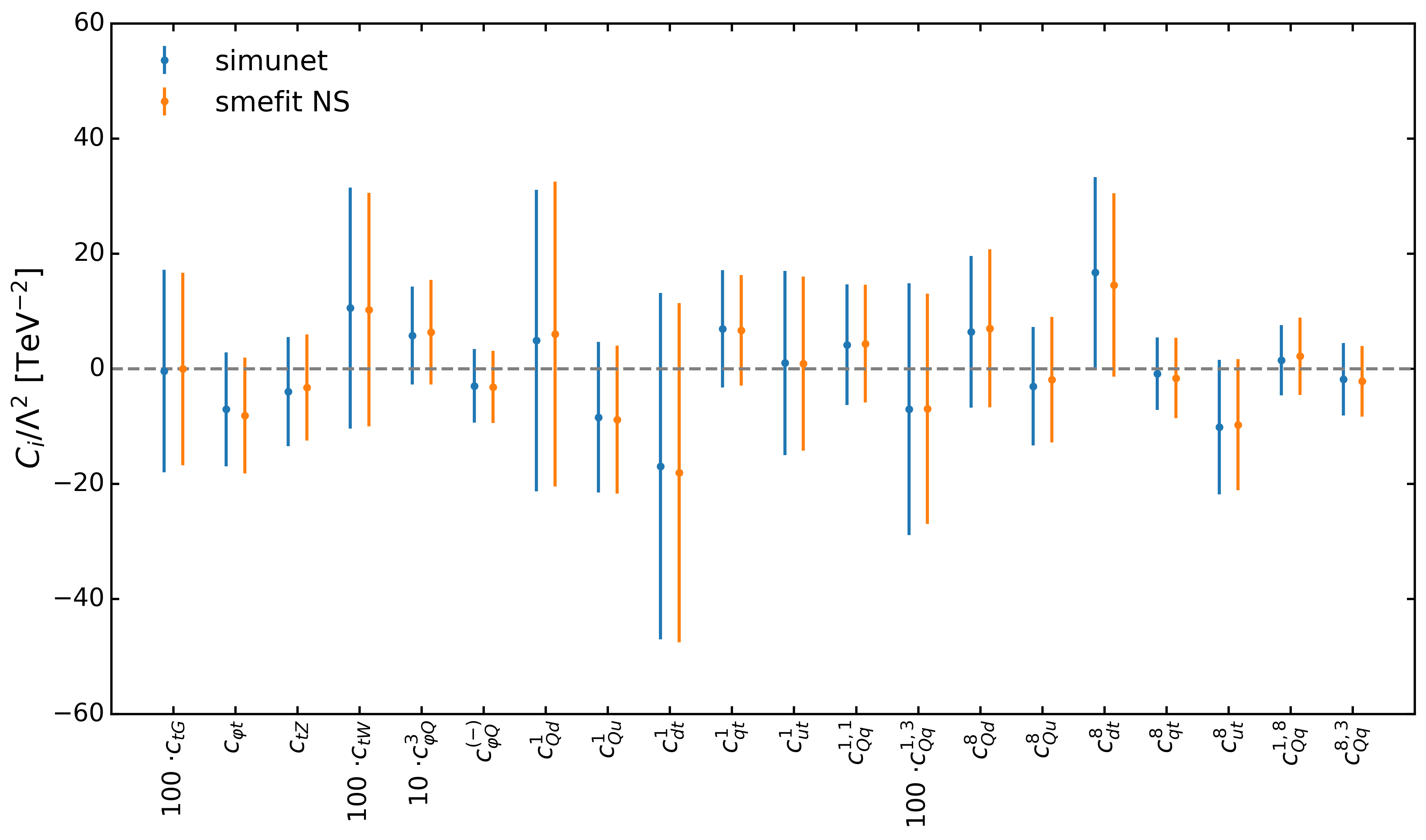
Figure C.1: Comparison between the 95% CL intervals obtained with SIMUnet in the fixed-PDF linear EFT case (full top quark dataset) with the corresponding results based on the SMEFiT framework (with the Nested Sampling option). In both cases the same experimental and theoretical inputs are adopted, see text for more details. These SIMUnet results coincide with those displayed in Fig. 6.4 in the fixed-PDF EFT analysis.

This benchmark study ensures that the optimisation algorithm adopted by SIMUnet is suitable both for PDF determinations (since it is based on the NNPDF4.0 settings) as well as for the determination of the EFT coefficients. The optimisation settings that provide the best performance of the SM-PDF and fixed-PDF EFT analyses are then combined for the simultaneous SMEFT-PDF extraction, where all weights of the SIMUnet network are allowed to be constrained by the data.

Appendix D Fit quality

Here we summarise the $\chi^{2}$ (computed using the experimental definition, Eq. 2.3) for the key PDF and EFT analyses presented in this work. Tables D.1, D.2 and D.3 display the values of the $\chi^{2}$ per data point for representative PDF and EFT fits, where for each dataset we also indicate the number of data points $n_{\rm dat}$. Specifically, we consider: (i) three SM-PDF fits: NNPDF4.0-notop , NNPDF4.0 , and Fit H in Table 4.1 (using our full top quark dataset); (ii) two fixed-PDF EFT fits, one based on NNPDF4.0-notop as input, and the other using Fit H as input; (iii) the outcome of the simultaneous SMEFT-PDF determination. We show sequentially the non-top datasets, the $t\bar{t}$ inclusive and associated production datasets, and the single-top inclusive and associated production datasets. We also provide the total $\chi^{2}$ for separate groups of processes, including the full non-top and top datasets, and well as for their total sum.

In Tables D.2 and D.3, entries in italics indicate datasets that do not enter the corresponding SM-PDF fit; for these datasets, we evaluate the associated $\chi^{2}$ values a posteriori using the resulting PDFs. For instance, all top data is removed from the NNPDF4.0-notop fit, and for some top quark observables such as four-heavy-quark production, PDF dependence is neglected. Furthermore, we note that the $\chi^{2}$ values for the NNPDF4.0-notop fit and for the fixed-PDF EFT fit based on NNPDF4.0-notop are identical in Table D.1, since the latter uses only top data as input. For the same reason, the entries in the columns for the SM-PDF Fit H and the fixed-PDF EFT fits based on Fit H are the same.

Dataset	$n_{\rm dat}$	$\chi^{2}/n_{\rm dat}$
		SM-PDF fits			Fixed-PDF EFT fits		SMEFT-PDFs
		NNPDF4.0 (no top)	NNPDF4.0	Fit H	NNPDF4.0 (no top)	Fit H	Joint fit
SLAC	67	0.768	0.758	0.753	0.768	0.753	0.761
BCDMS	581	1.265	1.247	1.251	1.265	1.251	1.245
NMC	325	1.298	1.306	1.304	1.298	1.304	1.292
CHORUS	832	0.899	0.900	0.901	0.899	0.901	0.898
NuTeV	76	0.398	0.425	0.423	0.398	0.423	0.393
HERA	1208	1.204	1.203	1.204	1.204	1.204	1.200
Total DIS	3089	1.122	1.119	1.119	1.122	1.119	1.114
E886 $\sigma^{d}_{\rm DY}/\sigma^{p}_{\rm DY}$	15	0.527	0.524	0.536	0.527	0.536	0.544
E886 $\sigma^{p}_{\rm DY}$	89	1.566	1.559	1.615	1.566	1.615	1.602
E605 $\sigma^{p}_{\rm DY}$	85	0.456	0.456	0.460	0.456	0.460	0.464
E906 $\sigma^{d}_{\rm DY}/\sigma^{p}_{\rm DY}$	6	0.827	0.885	0.886	0.827	0.886	0.955
Total fixed-target DY	195	0.981	0.979	1.008	0.981	1.008	1.006
CDF $d\sigma_{Z}/dy_{Z}$	28	1.234	1.280	1.275	1.234	1.275	1.188
D0 $d\sigma_{Z}/dy_{Z}$	28	0.637	0.644	0.640	0.637	0.640	0.632
D0 $W\to\mu\nu$ asy.	9	1.958	1.929	1.905	1.958	1.905	1.641
ATLAS low-mass DY 7 TeV	6	0.875	0.879	0.883	0.875	0.883	0.888
ATLAS high-mass DY 7 TeV	5	1.694	1.691	1.661	1.694	1.661	1.629
ATLAS $W,Z$ 7 TeV ($\mathcal{L}=35$ pb${}^{-1}$)	30	1.000	0.988	1.000	1.000	1.000	0.991
ATLAS $W,Z$ 7 TeV ($\mathcal{L}=4.6$ fb${}^{-1}$)	61	1.689	1.686	1.685	1.685	1.685	1.599
ATLAS low-mass DY 2D 8 TeV	60	1.203	1.216	1.225	1.203	1.225	1.207
ATLAS high-mass DY 2D 8 TeV	48	1.123	1.110	1.118	1.123	1.118	1.147
ATLAS $\sigma_{W,Z}^{\rm tot}$ 13 TeV	3	0.727	0.778	0.706	0.727	0.706	0.471
CMS $W$ electron asymmetry 7 TeV	11	0.836	0.833	0.836	0.836	0.836	0.892
CMS $W$ muon asymmetry 7 TeV	11	1.728	1.714	1.733	1.728	1.733	1.699
CMS DY 2D 7 TeV	110	1.367	1.361	1.353	1.367	1.353	1.339
CMS $W$ rapidity 8 TeV	22	1.375	1.361	1.365	1.375	1.365	1.162
LHCb $Z\rightarrow ee$ 7 TeV	9	1.630	1.648	1.636	1.630	1.636	1.669
LHCb $Z\rightarrow ee$ 8 TeV	17	1.272	1.325	1.334	1.272	1.334	1.266
LHCb $W,Z\rightarrow\mu$ 7 TeV	29	2.032	1.948	1.902	2.032	1.902	1.896
LHCb $W,Z\rightarrow\mu$ 8 TeV	30	1.494	1.426	1.417	1.494	1.417	1.386
LHCb $Z\rightarrow ee$ 13 TeV	15	1.701	1.726	1.717	1.701	1.717	1.640
LHCb $Z\rightarrow\mu\mu$ 13 TeV	16	0.970	0.993	0.978	0.970	0.978	0.928
Total inclusive gauge boson production	548	1.344	1.339	1.335	1.344	1.335	1.297
ATLAS $W^{\pm}+$jet 8 TeV	30	0.954	0.959	0.957	0.954	0.957	0.973
ATLAS $Z$ $p_{T}$ 8 TeV ($p_{T},m_{\ell\ell}$)	44	0.911	0.905	0.904	0.911	0.904	0.910
ATLAS $Z$ $p_{T}$ 8 TeV ($p_{T},y_{Z}$)	48	0.909	0.898	0.896	0.909	0.896	0.924
ATLAS incl. jets 8 TeV, $R=0.6$	171	0.682	0.687	0.687	0.682	0.687	0.667
ATLAS dijets 7 TeV, $R=0.6$	90	2.184	2.149	2.125	2.184	2.125	. 2.177
ATLAS isolated $\gamma$ prod. 13 TeV	53	0.811	0.763	0.753	0.811	0.753	0.813
CMS $Z$ $p_{T}$ 8 TeV	28	1.447	1.401	1.407	1.447	1.407	1.473
CMS incl. jets 8 TeV	185	1.140	1.183	1.200	1.140	1.200	1.118
CMS dijets 7 TeV	54	1.788	1.810	1.809	1.788	1.809	1.800
Total jets, $Z$ $p_{T}$ and isolated photon	703	1.154	1.157	1.158	1.154	1.158	1.148
Total non-top data	4535	1.148	1.145	1.146	1.148	1.146	1.137

Table D.1: The values of the $\chi^{2}$ per data point (using the experimental definition of Eq. (2.3)) for key PDF and EFT analyses presented in this work. For each dataset, we indicate the number of data points $n_{\rm dat}$ and the the $\chi^{2}$ values for i) three SM-PDF fits: NNPDF4.0-notop , NNPDF4.0 , and Fit H in Table 4.1 (full top quark dataset); ii) two fixed-PDF EFT fits: one based on NNPDF4.0-notop as input, and the other using Fit H as input; and finally iii) the outcome of the simultaneous SMEFT-PDF determination. Here we restrict ourselves to the non-top datasets considered in this analysis, the corresponding results for the top quark observables are provided in Tables D.2 and D.3. We also provide the total $\chi^{2}$ for separate groups of processes as well as for the full non-top dataset. The $\chi^{2}$ values for the NNPDF4.0-notop fit and for the fixed-PDF EFT fit based on NNPDF4.0-notop are identical, since the latter uses only top data as input. For the same reason, the entries in the columns for the SM-PDF Fit H and the fixed-PDF EFT fits based on Fit H are the same.

Dataset	$n_{\rm dat}$	$\chi^{2}/n_{\rm dat}$
		SM-PDF fits			Fixed-PDF EFT fits		SMEFT-PDFs
		NNPDF4.0 (no top)	NNPDF4.0	Fit H	NNPDF4.0 (no top)	Fit H	Joint fit
ATLAS $\sigma(t\bar{t})$, dilepton, 7 TeV	1	4.100	4.540	4.599	1.733	1.824	1.974
ATLAS $\sigma(t\bar{t})$, dilepton, 8 TeV	1	0.005	0.021	0.023	0.405	0.382	0.307
ATLAS $1/\sigma d\sigma/dm_{t\bar{t}}$, dilepton, 8 TeV	5	0.262	0.284	0.291	0.305	0.309	0.310
ATLAS $\sigma(t\bar{t})$, $\ell+$jets, 8 TeV	1	0.218	0.270	0.277	0.002	0.001	0.000
ATLAS $1/\sigma d\sigma/d|y_{t}|$, $\ell+$jets, 8 TeV	4	6.266	3.219	2.827	1.178	1.021	1.144
ATLAS $1/\sigma d\sigma/d|y_{t\bar{t}}|$, $\ell+$jets, 8 TeV	4	7.978	3.725	3.332	2.883	2.105	2.646
ATLAS $\sigma(t\bar{t})$, dilepton, 13 TeV	1	1.388	1.397	1.374	0.004	0.004	0.002
ATLAS $\sigma(t\bar{t})$, hadronic, 13 TeV	1	0.231	0.231	0.230	0.082	0.082	0.092
ATLAS $1/\sigma d^{2}\sigma/d|y_{t\bar{t}}|dm_{t\bar{t}}$, hadronic, 13 TeV	10	2.276	2.007	1.928	1.915	1.824	1.857
ATLAS $\sigma(t\bar{t})$, $\ell+$jets, 13 TeV	1	0.489	0.492	0.485	0.004	0.004	0.013
ATLAS $1/\sigma d\sigma/dm_{t\bar{t}}$, $\ell+$jets, 13 TeV	8	1.607	1.788	1.835	2.087	2.072	2.090
CMS $\sigma(t\bar{t})$, combined, 5 TeV	1	0.442	0.542	0.555	0.211	0.236	0.239
CMS $\sigma(t\bar{t})$, combined, 7 TeV	1	0.795	1.032	1.065	0.004	0.010	0.027
CMS $\sigma(t\bar{t})$, combined, 8 TeV	1	0.170	0.247	0.258	0.174	0.156	0.103
CMS $1/\sigma d^{2}\sigma/d|y_{t\bar{t}}|dm_{t\bar{t}}$, dilepton, 8 TeV	16	1.094	0.994	0.963	0.519	0.580	0.514
CMS $1/\sigma d\sigma/d|y_{t\bar{t}}|$, $\ell+$jets, 8 TeV	9	2.127	1.245	1.131	0.928	0.995	0.935
CMS $\sigma(t\bar{t})$, dilepton, 13 TeV	1	0.064	0.063	0.066	0.680	0.680	0.600
CMS $1/\sigma d\sigma/dm_{t\bar{t}}$, dilepton, 13 TeV	5	2.760	2.550	2.485	2.246	2.232	2.194
CMS $\sigma(t\bar{t})$, $\ell+$jets, 13 TeV	1	0.230	0.227	0.234	2.153	2.155	1.907
CMS $1/\sigma d\sigma/dm_{t\bar{t}}$, $\ell+$jets, 13 TeV	14	1.829	1.481	1.393	0.962	0.911	0.912
ATLAS charge asymmetry, 8 TeV	1	0.679	0.678	0.675	0.567	0.587	0.571
ATLAS charge asymmetry, 13 TeV	5	1.012	0.997	0.989	0.872	0.786	0.836
CMS charge asymmetry, 8 TeV	3	0.052	0.052	0.053	0.072	0.069	0.071
CMS charge asymmetry, 13 TeV	3	0.277	0.283	0.286	0.443	0.510	0.451
ATLAS & CMS combined charge asy., 8 TeV	6	0.603	0.602	0.602	0.646	0.659	0.651
ATLAS $W$-hel., 13 TeV	2	0.370	0.370	0.370	0.037	0.037	0.038
ATLAS & CMS combined $W$-hel., 8 TeV	2	1.046	1.046	1.046	0.853	0.853	0.854
Total inclusive $t\bar{t}$	108	1.700	1.328	1.271	1.032	0.994	1.002
ATLAS $\sigma(t\bar{t}Z)$, 8 TeV	1	0.264	0.232	0.235	1.331	1.161	1.258
ATLAS $\sigma(t\bar{t}W)$, 8 TeV	1	2.461	2.482	2.430	0.751	0.708	0.722
ATLAS $\sigma(t\bar{t}Z)$, 13 TeV	1	0.702	0.747	0.742	0.001	0.000	0.000
ATLAS $1/\sigma d\sigma(t\bar{t}Z)/dp_{T}^{Z}$, 13 TeV	5	1.961	1.940	1.933	1.870	1.840	1.860
ATLAS $\sigma(t\bar{t}W)$, 13 TeV	1	1.436	1.456	1.417	0.000	0.002	0.000
ATLAS $\sigma(t\bar{t}\gamma)$, 8 TeV	1	0.426	0.426	0.426	0.037	0.009	0.034
ATLAS $\sigma(t\bar{t}t\bar{t})$, multi-lepton, 13 TeV	1	3.655	3.655	3.655	4.289	3.784	4.145
ATLAS $\sigma(t\bar{t}t\bar{t})$, single lepton, 13 TeV	1	0.872	0.872	0.872	0.997	0.898	0.969
ATLAS $\sigma(t\bar{t}b\bar{b})$, $\ell+$jets, 13 TeV	1	2.062	2.062	2.062	1.093	1.316	1.152
CMS $\sigma(t\bar{t}Z)$, 8 TeV	1	0.432	0.470	0.466	0.005	0.020	0.010
CMS $\sigma(t\bar{t}W)$, 8 TeV	1	2.281	2.298	2.255	0.808	0.770	0.783
CMS $\sigma(t\bar{t}Z)$, 13 TeV	1	1.185	1.238	1.233	0.085	0.113	0.110
CMS $1/\sigma d\sigma(t\bar{t}Z)/dp_{T}^{Z}$, 13 TeV	3	0.628	0.598	0.590	0.936	0.756	0.898
CMS $\sigma(t\bar{t}W)$, 13 TeV	1	0.667	0.682	0.652	0.297	0.329	0.307
CMS $\sigma(t\bar{t}\gamma)$, 8 TeV	1	0.508	0.508	0.508	0.022	0.045	0.024
CMS $\sigma(t\bar{t}t\bar{t})$, multi-lepton, 13 TeV	1	0.027	0.027	0.027	0.124	0.041	0.096
CMS $\sigma(t\bar{t}t\bar{t})$, single lepton, 13 TeV	1	0.231	0.231	0.231	0.262	0.238	0.255
CMS $\sigma(t\bar{t}b\bar{b})$, all-jet, 13 TeV	1	1.878	1.878	1.878	1.334	1.466	1.369
CMS $\sigma(t\bar{t}b\bar{b})$, dilepton, 13 TeV	1	0.962	0.962	0.962	0.312	0.447	0.347
CMS $\sigma(t\bar{t}b\bar{b})$, $\ell+$jets, 13 TeV	1	0.900	0.900	0.900	0.135	0.269	0.167
Total associated $t\bar{t}$	26	1.255	1.255	1.246	0.925	0.888	0.913

Table D.2: Same as Table D.1 now for the inclusive and associated $t\bar{t}$ production datasets. Values in italics indicate datasets that do not enter the corresponding SM-PDF fit: for those processes, we evaluate a posteriori the physical observables and the associated $\chi^{2}$ values using the resulting PDFs from the fit. For instance, top data is removed from the NNPDF4.0-notop , and for some top quark observables like $t\bar{t}t\bar{t}$ their PDF dependence is neglected. The last row indicates the total values adding together the non-top and top data contributions to the $\chi^{2}$.

Dataset	$n_{\rm dat}$	$\chi^{2}/n_{\rm dat}$
		SM-PDF fits			Fixed-PDF EFT fits		SMEFT-PDFs
		NNPDF4.0 (no top)	NNPDF4.0	Fit H	NNPDF4.0 (no top)	Fit H	Joint fit
ATLAS $t$-channel $\sigma(t)$, 7 TeV	1	0.785	0.756	0.757	0.179	0.135	0.155
ATLAS $t$-channel $\sigma(\bar{t})$, 7 TeV	1	0.304	0.296	0.282	0.003	0.005	0.004
ATLAS $t$-channel $1/\sigma d\sigma(tq)/dy_{t}$, 7 TeV	3	0.909	0.959	0.971	0.885	0.946	0.900
ATLAS $t$-channel $1/\sigma d\sigma(\bar{t}q)/dy_{\bar{t}}$, 7 TeV	3	0.061	0.062	0.062	0.061	0.063	0.062
ATLAS $t$-channel $\sigma(t)$, 8 TeV	1	0.795	0.739	0.739	0.000	0.017	0.007
ATLAS $t$-channel $\sigma(\bar{t})$, 8 TeV	1	2.314	2.277	2.221	0.379	0.337	0.356
ATLAS $t$-channel $1/\sigma d\sigma(tq)/dy_{t}$, 8 TeV	3	0.288	0.246	0.241	0.290	0.245	0.283
ATLAS $t$-channel $1/\sigma d\sigma(\bar{t}q)/dy_{\bar{t}}$, 8 TeV	3	0.196	0.190	0.187	0.198	0.189	0.192
ATLAS $s$-channel $\sigma(t+\bar{t})$, 8 TeV	1	0.211	0.203	0.216	0.000	0.000	0.000
ATLAS $t$-channel $\sigma(t)$, 13 TeV	1	0.738	0.722	0.720	0.261	0.224	0.235
ATLAS $t$-channel $\sigma(\bar{t})$, 13 TeV	1	0.400	0.393	0.384	0.057	0.050	0.051
ATLAS $s$-channel $\sigma(t+\bar{t})$, 13 TeV	1	0.700	0.688	0.703	0.127	0.138	0.118
CMS $t$-channel $\sigma(t)+\sigma(\bar{t})$, 7 TeV	1	0.765	0.729	0.719	0.010	0.001	0.004
CMS $t$-channel $\sigma(t)$, 8 TeV	1	0.010	0.006	0.005	0.487	0.628	0.566
CMS $t$-channel $\sigma(\bar{t})$, 8 TeV	1	0.079	0.084	0.092	0.886	0.934	0.911
CMS $s$-channel $\sigma(t+\bar{t})$, 8 TeV	1	1.108	1.112	1.105	1.348	1.338	1.350
CMS $t$-channel $\sigma(t)$, 13 TeV	1	0.904	0.883	0.880	0.281	0.235	0.248
CMS $t$-channel $\sigma(\bar{t})$, 13 TeV	1	0.136	0.132	0.125	0.010	0.014	0.013
CMS $t$-channel $1/\sigma d\sigma/d|y^{(t)}|$, 13 TeV	4	0.412	0.387	0.383	0.405	0.378	0.396
Total single top	30	0.509	0.498	0.495	0.332	0.330	0.331
ATLAS $\sigma(tW)$, dilepton, 8 TeV	1	0.510	0.529	0.538	0.144	0.168	0.167
ATLAS $\sigma(tW)$, single-lepton, 8 TeV	1	0.695	0.708	0.713	0.428	0.449	0.448
ATLAS $\sigma(tW)$, dilepton, 13 TeV	1	1.150	1.149	1.148	0.840	0.847	0.849
ATLAS $\sigma_{\text{fid}}(tZj)$, dilepton, 13 TeV	1	0.115	0.115	0.115	0.871	0.611	0.795
CMS $\sigma(tW)$, dilepton, 8 TeV	1	0.359	0.371	0.376	0.134	0.150	0.149
CMS $\sigma(tW)$, dilepton, 13 TeV	1	0.434	0.437	0.438	1.612	1.573	1.563
CMS $\sigma_{\text{fid}}(tZj)$, dilepton, 13 TeV	1	1.041	1.041	1.041	0.279	0.427	0.316
CMS $d\sigma_{\text{fid}}(tZj)/dp_{T}^{t}$, dilepton, 13 TeV	3	0.362	0.362	0.362	0.130	0.156	0.134
CMS $\sigma(tW)$, single-lepton, 13 TeV	1	2.837	2.833	2.832	1.817	1.839	1.846
Total associated single top	11	0.748	0.752	0.753	0.592	0.594	0.594
Total top	175	1.370	1.139	1.102	0.868	0.839	0.848
Total dataset	4710	1.156	1.145	1.144	1.138	1.135	1.126

Table D.3: Same as Table D.2 now for the inclusive and associated single-top production datasets. Values in italics indicate datasets that do not enter the corresponding fits: for those processes, we evaluate a posteriori the physical observables and the associated $\chi^{2}$ values using the resulting PDFs from the fit. The last row indicates the total values adding together the non-top and top data contributions to the $\chi^{2}$, and the next-to-last row the total top quark contribution.

Several observations can be drawn from the results presented in Tables D.1, D.2 and D.3. First of all, we note that the description of the non-top data is improved in the simultaneous SMEFT-PDF analysis, with $\chi^{2}=1.137$ to be compared with the analogous SM-PDF analysis (Fit H) which leads to $\chi^{2}=1.146$. Given that we have $n_{\rm dat}=4535$ no-top data points, this improvement corresponds to 40 units in the absolute $\chi^{2}$. This improvement cannot traced back to a specific measurements or group of processes. In turn, this improvement is also reflected for the full dataset, whose $\chi^{2}$ is the lowest (1.126 for $n_{\rm dat}=4710$ points) in the SMEFT-PDF analysis. This lower $\chi^{2}$ as compared to the SM-PDF baseline fits is not surprising, taking into account the fact that (as discussed in Sect. 5) we now have more degrees of freedom in the fit, and in particular the inclusion of linear EFT corrections is instrumental in improving the $\chi^{2}$ to the top quark data as compared to the SM-PDF fits. We also find that the fit quality to the top datasets is similar in the joint SMEFT-PDF analysis and in the fixed-PDF EFT fits with either NNPDF4.0-notop or Fit H as input PDFs, with $\chi^{2}=0.848,0.868,0.839$ respectively in each case for $n_{\rm dat}=175$. The small differences between the three cases (less than five units in absolute $\chi^{2}$) are consistent with the reported independence of the EFT interpretation of top quark data with respect to the choice of input PDF in the calculation.

Finally, we note the only class of top quark production process for which the $\chi^{2}$ values are markedly different in the SM-PDF fits is inclusive top quark pair production. Indeed, the $\chi^{2}$ values for the complete top quark dataset are $1.370,1.139$, and $1.102$ in the SM-PDF fits without top data, with NNPDF4.0 , and with the full top quark dataset (Fit H) respectively; this improvement arises mostly from the $t\bar{t}$ group, whose $\chi^{2}$ values are $1.700,1.328$, and $1.271$ for the same three fits respectively. This observation is consistent with the findings of Sect. 4, that the dominant PDF sensitivity in Fit H arises from inclusive $t\bar{t}$ production. We also note that the $\chi^{2}$ for top quark data is similar between NNPDF4.0 and Fit H, again in agreement with the fact that the additional top quark measurements considered here as compared to those in NNPDF4.0 have a consistent pull on the PDFs, in particular on the large-$x$ gluon.

Appendix E Pitfalls of the Monte-Carlo replica method for quadratic EFT fits

This analysis was originally prepared with the intention of performing a fully simultaneous SMEFT-PDF fit using NLO QCD theory, including quadratic, $\mathcal{O}\left(\Lambda^{-4}\right)$, contributions from the SMEFT. To this end, the capabilities of the SIMUnet framework were extended, as discussed in Sect. 3.2, and all necessary SMEFT $K$-factors needed for the quadratic predictions were produced. However, whilst benchmarking our code, we noticed significant disagreement between quadratic SMEFT-only fits produced using the SIMUnet methodology and the SMEFiT Nested Sampling option; on the other hand, we note perfect agreement between our SIMUnet quadratic SMEFT-only fits and the SMEFiT MCfit option.

This disagreement can be traced back to a deficiency in the Monte-Carlo sampling method used to propagate experimental error to the SMEFT coefficients, which currently prevents us from applying the the SIMUnet framework to joint SMEFT-PDF fits with quadratic EFT calculations. In this Appendix, we describe our current understanding of these limitations within the context of a toy model, and give a more realistic example from this work; further work on the topic is deferred to a future publication..

E.1 A toy model for quadratic EFT fits

In the following subsection, we consider a toy scenario involving a single data point $d$ and only one Wilson coefficient $c$ (we ignore all PDF-dependence). We suppose that our observed experimental data point $d$ is a random variable drawn from a normal distribution centred on the underlying quadratic theory prediction, and with experimental variance $\sigma^{2}$:

$$d\sim N(t(c),\sigma^{2}).$$ (E.1)

We assume that the theory prediction is quadratic in the SMEFT Wilson coefficient $c$, taking the form:

$$t(c)=t^{\text{SM}}+ct^{\text{lin}}+c^{2}t^{\text{quad}}\,,$$ (E.2)

where we set $\Lambda=1$ TeV for convenience. Recall that $t^{\text{quad}}>0$, since it corresponds to a squared amplitude. Given the observed data $d$, we would like to construct interval estimates for the parameter $c$ (usually confidence intervals in a frequentist setting or credible intervals in a Bayesian setting). Here, we shall describe the analytical construction of two interval estimates: first, using the Bayesian method, and second, using the Monte-Carlo replica method.

Bayesian method.

In the Bayesian approach, $c$ is treated as a random variable with its own distribution. By Bayes’ theorem, we can write the probability distribution of $c$, given the observed data $d$, up to a proportionality constant (given by $1/\mathbb{P}(d)$, where $\mathbb{P}(d)$ is called the Bayes’ evidence) as:

$$\mathbb{P}(c|d)\propto\mathbb{P}(d|c)\mathbb{P}(c),$$ (E.3)

where $\mathbb{P}(c|d)$ is called the posterior distribution of $c$, given the observed data $d$, and $\mathbb{P}(c)$ is called the prior distribution of $c$ - this is our initial ‘best guess’ of the distribution of $c$ before the observation of the data takes place. This distribution is often taken to be uniform in SMEFT fits; we shall assume this here.

Given a value of $c$, the distribution $\mathbb{P}(d|c)$ of the data $d$ is assumed to be Gaussian, as specified in Eq. (E.1). In particular, we can deduce that the posterior distribution of $c$ obeys the following proportionality relation:

$$\mathbb{P}(c|d)\propto\exp\left(-{{1}\over{2\sigma^{2}}}\left(d-t(c)\right)^{2}\right).$$ (E.4)

This posterior distribution can be used to place interval estimates on the parameter $c$. One way of doing this is to construct highest density intervals. These are computed as follows. For a $100\alpha$% credible interval, we determine the constant $p(\alpha)$ satisfying:

$$\int\limits_{\{c:\leavevmode\nobreak\ \mathbb{P}(c|d)>p(\alpha)\}}\mathbb{P}(c|d)\ dc=\alpha.$$ (E.5)

An interval estimate for $c$ is then given by $\{c:\mathbb{P}(c|d)>p(\alpha)\}$. In order to obtain such intervals then, we must construct the posterior $\mathbb{P}(c|d)$; efficient sampling from the posterior is guaranteed by methods such as Nested Sampling [187, 188].

The Monte-Carlo replica method.

This method takes a different approach in order to produce a posterior distribution for the parameter $c$. Given the observed central data value $d$, one samples repeatedly from the normal distribution $N(d,\sigma^{2})$ to generate a collection of pseudodata replicas, which we shall denote as $d^{(1)},...,d^{(N_{\text{rep}})}$, where $N_{\text{rep}}$ is the total number of replicas. Given a pseudodata replica $d^{(i)}$, one obtains a corresponding best-fit value of the Wilson coefficient parameter $c^{(i)}$ by minimising the $\chi^{2}$ of the theory to the pseudodata:

$$c^{(i)}=\operatorname*{arg\,min}_{c}\chi^{2}(c,d^{(i)})=\operatorname*{arg\,min}_{c}\left({{(d^{(i)}-t(c))^{2}}\over{\sigma^{2}}}\right).$$ (E.6)

In this toy scenario, we can determine an analytical formula for $c^{(i)}$:

$$c^{(i)}=\begin{cases}\displaystyle-{{t^{\text{lin}}}\over{2t^{\text{quad}}}},&\text{if $d^{(i)}\leq\left(t^{\text{SM}}-(t^{\text{lin}})^{2}/4t^{\text{quad}}\right)$ ;}\\[8.61108pt] \displaystyle{{-t^{\text{lin}}\pm\sqrt{(t^{\text{lin}})^{2}-4t^{\text{quad}}(t^{\text{SM}}-d^{(i)})}}\over{2t^{\text{quad}}}},&\text{if $d^{(i)}\geq\left(t^{\text{SM}}-(t^{\text{lin}})^{2}/4t^{\text{quad}}\right)$ \, .}\end{cases}$$ (E.7)

The first case arises when the $\chi^{2}$ to the pseudodata $d^{(i)}$ has a single minimum, whilst the second case arises when the $\chi^{2}$ has two minima. The two cases are split based on the value of

$$t_{\text{min}}=t^{\text{SM}}-(t^{\text{lin}})^{2}/4t^{\text{quad}}\,,$$ (E.8)

which is the minimum value of the quadratic theory prediction $t(c)=t^{\text{SM}}+ct^{\text{lin}}+c^{2}t^{\text{quad}}$. Note that for data replicas such that $d^{(i)}\leq t_{\text{min}}$, the best-fit value $c^{(i)}$ becomes independent of $d^{(i)}$ and depends only on the ratio between linear and quadratic EFT cross-sections.

Now, given that $d^{(i)}$ is a random variable drawn from the normal distribution $N(d,\sigma^{2})$, one can infer the corresponding distribution of the random variable $c^{(i)}$, which is a function of the pseudodata $d^{(i)}$. For a real random variable $X$ with associated probability density $P_{X}(x)$, a function $f:\mathbb{R}\rightarrow\mathbb{R}$ of the random variable has the distribution:

$$P_{f(X)}(y)=\int\limits_{-\infty}^{\infty}dx\ P_{X}(x)\delta(y-f(x)).$$ (E.9)

In our case, $c^{(i)}$ is a multi-valued function of $d^{(i)}$ given the two square roots, but the formula is easily generalised to this case. Recalling that the pseudodata replicas are generated according to a Gaussian distribution around the central measurement $d$ with variance $\sigma^{2}$, we find that the probability density function for the Wilson coefficient replica $c^{(i)}$ is given (up to a proportionality constant) by:

$$P_{c^{(i)}}(c) \propto\int\limits_{-\infty}^{t_{\text{min}}}dx\ \delta\left(c+{{t^{\text{lin}}}\over{2t^{\text{quad}}}}\right)\exp\left(-{{1}\over{2\sigma^{2}}}(x-d)^{2}\right)$$

$$\qquad+\int\limits_{t_{\text{min}}}^{\infty}dx\ \delta\left(c-\left({{-t^{\text{lin}}+\sqrt{(t^{\text{lin}})^{2}-4t^{\text{quad}}(t^{\text{SM}}-x)}}\over{2t^{\text{quad}}}}\right)\right)\exp\left(-{{1}\over{2\sigma^{2}}}(x-d)^{2}\right)$$

$$\qquad+\int\limits_{t_{\text{min}}}^{\infty}dx\ \delta\left(c-\left({{-t^{\text{lin}}-\sqrt{(t^{\text{lin}})^{2}-4t^{\text{quad}}(t^{\text{SM}}-x)}}\over{2t^{\text{quad}}}}\right)\right)\exp\left(-{{1}\over{2\sigma^{2}}}(x-d)^{2}\right).$$ (E.10)

Simplifying the delta functions in the second and third integrals, we find:

$$P_{c^{(i)}}(c)\propto\delta\left(c+{{t^{\text{lin}}}\over{2t^{\text{quad}}}}\right)\int\limits_{-\infty}^{t_{\text{min}}}dx\ \exp\left(-{{1}\over{2\sigma^{2}}}(x-d)^{2}\right)+{{2}\over{|2ct^{\text{quad}}+t^{\text{lin}}|}}\exp\left(-{{1}\over{2\sigma^{2}}}(d-t(c))^{2}\right)\,.$$ (E.11)

This result is different from the posterior distribution obtained by the Bayesian method in Eq. (E.4). Notable features of the posterior distribution $P_{c^{(i)}}(c)$ are: (i) the distribution has a Dirac-delta peak at $c=-t^{\text{lin}}/2t^{\text{quad}}$; (ii) elsewhere, the distribution is given by the Bayesian posterior distribution rescaled by a prefactor dependent on $c$. Therefore, the Monte Carlo replica optimisation method will not in general reproduce the Bayesian posterior.

However, one can note that in an appropriate limit, the Bayesian posterior is indeed recovered. In particular, suppose that the quadratic EFT cross-section is subdominant compared to the linear term, $t^{\text{lin}}\gg t^{\text{quad}}$; in this case, we have that $t_{\text{min}}\rightarrow-\infty$ so that the first term in Eq. (E.11) vanishes and the prefactor of the second term can be approximated with $2ct^{\text{quad}}+t^{\text{lin}}\approx t^{\text{lin}}$. Thus, the Bayesian posterior from Eq. (E.4) is indeed recovered, and we see that the two methods are formally identical for a linear EFT analysis. Further, it is possible to show analytically that for multiple SMEFT parameters and multiple correlated data points, if only linear theory is used the two distributions agree exactly.

This calculation demonstrates that, for quadratic EFT fits, the Monte-Carlo replica method will not in general reproduce the Bayesian posteriors that one would obtain from, say, a nested sampling approach; agreement will only occur provided quadratic EFT corrections are sufficiently subdominant in comparison with the linear ones. For this reason, in this work we restrict the SMEFT-PDF fits based on SIMUnet (which rely on the use of the Monte-Carlo replica method) to linear EFT calculations; we defer the further investigation of the use of the Monte-Carlo replica method, and how it might be modified for use in SIMUnet, to future works.

E.2 Application to one-parameter fits

As demonstrated above, the Monte-Carlo replica method will lead to posterior distributions differing from their Bayesian counterparts whenever quadratic EFT corrections dominate over linear ones. Here, we show the numerical impact of these differences in a model case, namely the one-parameter fit of the coefficient $c_{dt}^{8}$ to the CMS 13 TeV $t\bar{t}$ invariant mass distribution measurement based on the $\ell+$jets final-state [106]. Fig. E.1 compares the experimental data from this measurement with the corresponding SM theory calculations at NNLO using the NNPDF4.0 (no top) PDF set as input. We observe that the SM theory predictions overshoot the data, especially in the high $m_{t\bar{t}}$ regions, where energy-growing effects enhance the EFT corrections. Given that the pseudodata replicas $d^{(i)}$ are fluctuated around the central value $d$, the configuration where the SM overshoots the data potentially enhances the contribution of the upper solution in Eq. (E.7) leading to the Dirac delta peak in the posterior Eq. (E.11).

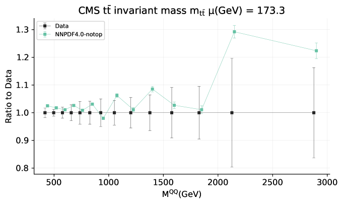
Figure E.1: Comparison between the experimental data for the top-quark pair invariant mass $m_{t\bar{t}}$ distribution from the $\ell+$jets CMS measurement at 13 TeV [106], with the corresponding SM theory calculations at NNLO using the NNPDF4.0 (no top) PDF set as input. For the latter, the error band indicates the PDF uncertainties, and for the former the diagonal entries of the experimental covariance matrix. Results are shown as ratios to the central value of the data. The SM theory predictions overshoot the data, especially in the high $m_{t\bar{t}}$ regions, where energy-growing effects enhance the EFT corrections.

For the case of the $c_{dt}^{8}$ coefficient, the quadratic EFT corrections dominate over the linear ones and hence the net effect of a non-zero coefficient is typically an upwards shift of the theory prediction. Indeed, we have verified that for this coefficient the biggest negative correction one can obtain is of order $\sim 2\%$. For the last $m_{t\bar{t}}$ bin, the minimum of the theory cross section $t_{\rm min}$ in Eq. (E.8) is obtained for a value $c_{dt}^{8}\approx-0.2$, while for the second to last bin instead $t_{\rm min}$ is minimised by $c_{dt}^{8}\approx-0.3$. The combination of these two features (a dominant quadratic EFT term, and a SM prediction overshooting the data) suggests that the Monte-Carlo replica method’s posterior will be enhanced for $c_{dt}^{8}\in(-0.3,-0.2)$ as compared to the Bayesian posterior.

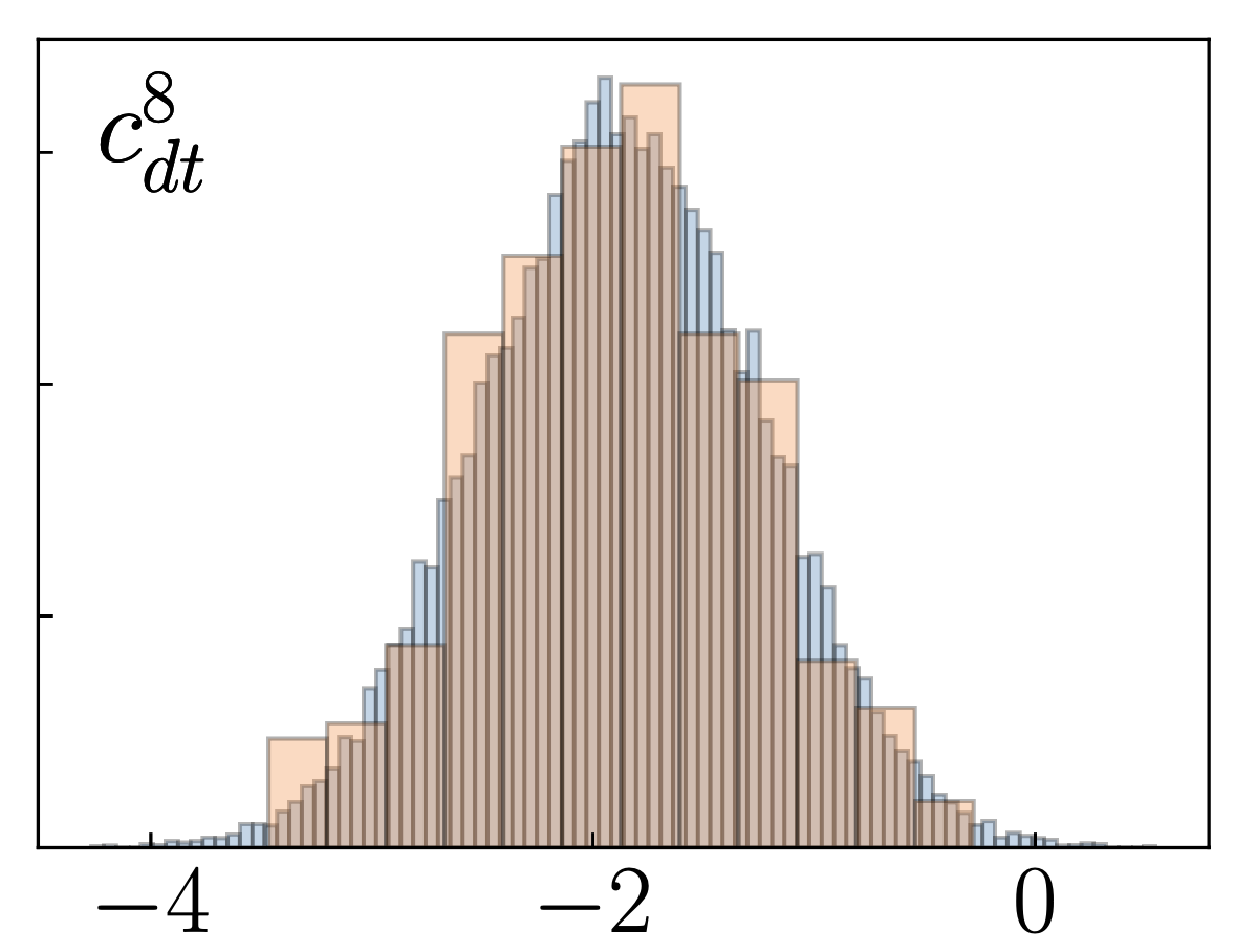
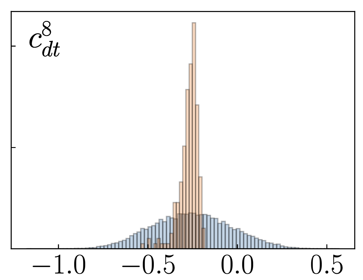
Figure E.2: Posterior distributions for a one-parameter fit of the four-fermion coefficient $c_{dt}^{8}$ with the sole experimental input being the CMS $m_{t\bar{t}}$ distribution displayed in Fig. E.1. Results are obtained with SMEFiT and we compare the outcome of Nested Sampling (in blue) with that of MCfit (in red) for linear (left panel) and quadratic (right panel) EFT fits.

In Fig. E.2 we compare the posterior distributions for a one-parameter fit of the four-fermion coefficient $c_{dt}^{8}$ with the sole experimental input being the CMS $m_{t\bar{t}}$ distribution displayed in Fig. E.1. Results are obtained with SMEFiT and we compare the outcome of Nested Sampling (in blue) with that of MCfit (in red) for linear and quadratic EFT fits. The agreement in the linear fit is lost for its quadratic counterpart, with the main difference being a sharp peak in the region $c_{dt}^{8}\in(-0.3,-0.2)$ in which the contribution from the delta function in Eq. E.11 is most marked.

The scenario displayed in Fig. E.2 is chosen to display the maximum effect, based on a single coefficient with large quadratic EFT corrections, and a dataset where the SM overshoots the data in the $m_{t\bar{t}}$ region where EFT effects are the largest. Within a global fit, these differences are partially washed out (indeed the Bayesian and MCfit posterior distributions mostly agree well for the quadratic SMEFiT analysis, as shown in [171], for the majority of fitted coefficients). Nevertheless, at least in its current implementation, Fig. E.2 highlights that the Monte-Carlo replica method is affected by pitfalls that prevent its straightforward application to global EFT interpretations of experimental data which include quadratic corrections.

References

- [1] G. Isidori, G. Ridolfi, and A. Strumia, “On the metastability of the standard model vacuum,” Nucl. Phys. B 609 (2001) 387–409, arXiv:hep-ph/0104016.
- [2] D. Buttazzo, G. Degrassi, P. P. Giardino, G. F. Giudice, F. Sala, A. Salvio, and A. Strumia, “Investigating the near-criticality of the Higgs boson,” JHEP 12 (2013) 089, arXiv:1307.3536 [hep-ph].
- [3] L. Di Luzio, G. Isidori, and G. Ridolfi, “Stability of the electroweak ground state in the Standard Model and its extensions,” Phys. Lett. B 753 (2016) 150–160, arXiv:1509.05028 [hep-ph].
- [4] CDF Collaboration, F. Abe et al., “Observation of top quark production in collisions,” Phys. Rev. Lett. 74 (1995) 2626–2631, arXiv:hep-ex/9503002.
- [5] D0 Collaboration, S. Abachi et al., “Observation of the top quark,” Phys. Rev. Lett. 74 (1995) 2632–2637, arXiv:hep-ex/9503003.
- [6] CMS Collaboration, S. Chatrchyan et al., “Determination of the Top-Quark Pole Mass and Strong Coupling Constant from the Production Cross Section in Collisions at = 7 TeV,” Phys. Lett. B 728 (2014) 496–517, arXiv:1307.1907 [hep-ex]. [Erratum: Phys.Lett.B 738, 526–528 (2014)].
- [7] A. M. Cooper-Sarkar, M. Czakon, M. A. Lim, A. Mitov, and A. S. Papanastasiou, “Simultaneous extraction of and from LHC differential distributions,” arXiv:2010.04171 [hep-ph].
- [8] CMS Collaboration, A. M. Sirunyan et al., “Measurement of CKM matrix elements in single top quark -channel production in proton-proton collisions at 13 TeV,” Phys. Lett. B 808 (2020) 135609, arXiv:2004.12181 [hep-ex].
- [9] ATLAS Collaboration, “Measurement of the top-quark mass using a leptonic invariant mass in collisions at with the ATLAS detector,” arXiv:2209.00583 [hep-ex].
- [10] CMS Collaboration, “Measurement of the top quark mass using a profile likelihood approach with the lepton+jets final states in proton-proton collisions at = 13 TeV,” arXiv:2302.01967 [hep-ex].
- [11] J. Gao, L. Harland-Lang, and J. Rojo, “The Structure of the Proton in the LHC Precision Era,” Phys. Rept. 742 (2018) 1–121, arXiv:1709.04922 [hep-ph].
- [12] S. Amoroso et al., “Snowmass 2021 whitepaper: Proton structure at the precision frontier,” Acta Phys. Polon. B 53 no. 12, (2022) A1, arXiv:2203.13923 [hep-ph].
- [13] M. Czakon, M. L. Mangano, A. Mitov, and J. Rojo, “Constraints on the gluon PDF from top quark pair production at hadron colliders,” JHEP 1307 (2013) 167, arXiv:1303.7215 [hep-ph].
- [14] M. Czakon, N. P. Hartland, A. Mitov, E. R. Nocera, and J. Rojo, “Pinning down the large-x gluon with NNLO top-quark pair differential distributions,” JHEP 04 (2017) 044, arXiv:1611.08609 [hep-ph].
- [15] M. Czakon, S. Dulat, T.-J. Hou, J. Huston, A. Mitov, A. S. Papanastasiou, I. Sitiwaldi, Z. Yu, and C. P. Yuan, “An exploratory study of the impact of CMS double-differential top distributions on the gluon parton distribution function,” J. Phys. G 48 no. 1, (2020) 015003, arXiv:1912.08801 [hep-ph].
- [16] E. R. Nocera, M. Ubiali, and C. Voisey, “Single Top Production in PDF fits,” JHEP 05 (2020) 067, arXiv:1912.09543 [hep-ph].
- [17] J. Campbell, T. Neumann, and Z. Sullivan, “Testing parton distribution functions with t-channel single-top-quark production,” Phys. Rev. D 104 no. 9, (2021) 094042, arXiv:2109.10448 [hep-ph].
- [18] M. Czakon, D. Heymes, and A. Mitov, “Dynamical scales for multi-TeV top-pair production at the LHC,” JHEP 04 (2017) 071, arXiv:1606.03350 [hep-ph].
- [19] M. Czakon, A. Mitov, and R. Poncelet, “NNLO QCD corrections to leptonic observables in top-quark pair production and decay,” JHEP 05 (2021) 212, arXiv:2008.11133 [hep-ph].
- [20] M. Czakon, D. Heymes, A. Mitov, D. Pagani, I. Tsinikos, and M. Zaro, “Top-pair production at the LHC through NNLO QCD and NLO EW,” arXiv:1705.04105 [hep-ph].
- [21] M. Czakon, A. Ferroglia, D. Heymes, A. Mitov, B. D. Pecjak, D. J. Scott, X. Wang, and L. L. Yang, “Resummation for (boosted) top-quark pair production at NNLO+NNLL’ in QCD,” JHEP 05 (2018) 149, arXiv:1803.07623 [hep-ph].
- [22] J. Mazzitelli, P. F. Monni, P. Nason, E. Re, M. Wiesemann, and G. Zanderighi, “Top-pair production at the LHC with MINNLO,” JHEP 04 (2022) 079, arXiv:2112.12135 [hep-ph].
- [23] E. L. Berger, J. Gao, and H. X. Zhu, “Differential Distributions for t-channel Single Top-Quark Production and Decay at Next-to-Next-to-Leading Order in QCD,” JHEP 11 (2017) 158, arXiv:1708.09405 [hep-ph].
- [24] E. L. Berger, J. Gao, C. P. Yuan, and H. X. Zhu, “NNLO QCD Corrections to t-channel Single Top-Quark Production and Decay,” Phys. Rev. D 94 no. 7, (2016) 071501, arXiv:1606.08463 [hep-ph].
- [25] Z. L. Liu and J. Gao, “s -channel single top quark production and decay at next-to-next-to-leading-order in QCD,” Phys. Rev. D 98 no. 7, (2018) 071501, arXiv:1807.03835 [hep-ph].
- [26] D. Barducci et al., “Interpreting top-quark LHC measurements in the standard-model effective field theory,” arXiv:1802.07237 [hep-ph].
- [27] A. Buckley, C. Englert, J. Ferrando, D. J. Miller, L. Moore, M. Russell, and C. D. White, “Constraining top quark effective theory in the LHC Run II era,” JHEP 04 (2016) 015, arXiv:1512.03360 [hep-ph].
- [28] I. Brivio, S. Bruggisser, F. Maltoni, R. Moutafis, T. Plehn, E. Vryonidou, S. Westhoff, and C. Zhang, “O new physics, where art thou? A global search in the top sector,” JHEP 02 (2020) 131, arXiv:1910.03606 [hep-ph].
- [29] S. Bißmann, J. Erdmann, C. Grunwald, G. Hiller, and K. Kröninger, “Constraining top-quark couplings combining top-quark and decay observables,” Eur. Phys. J. C 80 no. 2, (2020) 136, arXiv:1909.13632 [hep-ph].
- [30] N. P. Hartland, F. Maltoni, E. R. Nocera, J. Rojo, E. Slade, E. Vryonidou, and C. Zhang, “A Monte Carlo global analysis of the Standard Model Effective Field Theory: the top quark sector,” JHEP 04 (2019) 100, arXiv:1901.05965 [hep-ph].
- [31] G. Durieux, A. Irles, V. Miralles, A. Peñuelas, R. Pöschl, M. Perelló, and M. Vos, “The electro-weak couplings of the top and bottom quarks — Global fit and future prospects,” JHEP 12 (2019) 98, arXiv:1907.10619 [hep-ph]. [Erratum: JHEP 01, 195 (2021)].
- [32] S. van Beek, E. R. Nocera, J. Rojo, and E. Slade, “Constraining the SMEFT with Bayesian reweighting,” SciPost Phys. 7 no. 5, (2019) 070, arXiv:1906.05296 [hep-ph].
- [33] B. R. Yates, “Using associated top quark production to probe for new physics within the framework of effective field theory,” in 13th International Workshop on Top Quark Physics. 1, 2021. arXiv:2101.10828 [hep-ex].
- [34] S. Carrazza, C. Degrande, S. Iranipour, J. Rojo, and M. Ubiali, “Can New Physics hide inside the proton?,” Phys. Rev. Lett. 123 no. 13, (2019) 132001, arXiv:1905.05215 [hep-ph].
- [35] A. Greljo, S. Iranipour, Z. Kassabov, M. Madigan, J. Moore, J. Rojo, M. Ubiali, and C. Voisey, “Parton distributions in the SMEFT from high-energy Drell-Yan tails,” JHEP 07 (2021) 122, arXiv:2104.02723 [hep-ph].
- [36] D. Liu, C. Sun, and J. Gao, “Machine learning of log-likelihood functions in global analysis of parton distributions,” JHEP 08 (2022) 088, arXiv:2201.06586 [hep-ph].
- [37] J. Gao, M. Gao, T. J. Hobbs, D. Liu, and X. Shen, “Simultaneous CTEQ-TEA extraction of PDFs and SMEFT parameters from jet and data,” arXiv:2211.01094 [hep-ph].
- [38] CMS Collaboration, A. Tumasyan et al., “Measurement and QCD analysis of double-differential inclusive jet cross sections in proton-proton collisions at = 13 TeV,” JHEP 02 (2022) 142, arXiv:2111.10431 [hep-ex]. [Addendum: JHEP 12, 035 (2022)].
- [39] S. Iranipour and M. Ubiali, “A new generation of simultaneous fits to LHC data using deep learning,” JHEP 05 (2022) 032, arXiv:2201.07240 [hep-ph].
- [40] NNPDF Collaboration, R. D. Ball et al., “The path to proton structure at 1% accuracy,” Eur. Phys. J. C 82 no. 5, (2022) 428, arXiv:2109.02653 [hep-ph].
- [41] NNPDF Collaboration, R. D. Ball et al., “An open-source machine learning framework for global analyses of parton distributions,” Eur. Phys. J. C 81 no. 10, (2021) 958, arXiv:2109.02671 [hep-ph].
- [42] SMEFiT Collaboration, J. J. Ethier, G. Magni, F. Maltoni, L. Mantani, E. R. Nocera, J. Rojo, E. Slade, E. Vryonidou, and C. Zhang, “Combined SMEFT interpretation of Higgs, diboson, and top quark data from the LHC,” JHEP 11 (2021) 089, arXiv:2105.00006 [hep-ph].
- [43] New Muon Collaboration, M. Arneodo et al., “Accurate measurement of and ,” Nucl. Phys. B487 (1997) 3–26, arXiv:hep-ex/9611022.
- [44] New Muon Collaboration, M. Arneodo et al., “Measurement of the proton and deuteron structure functions, and , and of the ratio ,” Nucl. Phys. B483 (1997) 3–43, arXiv:hep-ph/9610231.
- [45] L. W. Whitlow, E. M. Riordan, S. Dasu, S. Rock, and A. Bodek, “Precise measurements of the proton and deuteron structure functions from a global analysis of the SLAC deep inelastic electron scattering cross-sections,” Phys. Lett. B282 (1992) 475–482.
- [46] BCDMS Collaboration, A. C. Benvenuti et al., “A High Statistics Measurement of the Proton Structure Functions and from Deep Inelastic Muon Scattering at High ,” Phys. Lett. B223 (1989) 485.
- [47] CHORUS Collaboration, G. Onengut et al., “Measurement of nucleon structure functions in neutrino scattering,” Phys. Lett. B632 (2006) 65–75.
- [48] NuTeV Collaboration, M. Goncharov et al., “Precise measurement of dimuon production cross-sections in Fe and Fe deep inelastic scattering at the Tevatron,” Phys. Rev. D64 (2001) 112006, arXiv:hep-ex/0102049.
- [49] D. A. Mason, “Measurement of the strange - antistrange asymmetry at NLO in QCD from NuTeV dimuon data,”. FERMILAB-THESIS-2006-01.
- [50] ZEUS, H1 Collaboration, H. Abramowicz et al., “Combination of measurements of inclusive deep inelastic scattering cross sections and QCD analysis of HERA data,” Eur. Phys. J. C75 no. 12, (2015) 580, arXiv:1506.06042 [hep-ex].
- [51] H1, ZEUS Collaboration, H. Abramowicz et al., “Combination and QCD analysis of charm and beauty production cross-section measurements in deep inelastic scattering at HERA,” Eur. Phys. J. C78 no. 6, (2018) 473, arXiv:1804.01019 [hep-ex].
- [52] G. Moreno et al., “Dimuon production in proton - copper collisions at = 38.8-GeV,” Phys. Rev. D43 (1991) 2815–2836.
- [53] NuSea Collaboration, J. C. Webb et al., “Absolute Drell-Yan dimuon cross sections in 800-GeV/c p p and p d collisions,” arXiv:hep-ex/0302019.
- [54] FNAL E866/NuSea Collaboration, R. S. Towell et al., “Improved measurement of the anti-d/anti-u asymmetry in the nucleon sea,” Phys. Rev. D64 (2001) 052002, arXiv:hep-ex/0103030.
- [55] CDF Collaboration, T. A. Aaltonen et al., “Measurement of of Drell-Yan pairs in the Mass Region from Collisions at TeV,” Phys. Lett. B692 (2010) 232–239, arXiv:0908.3914 [hep-ex].
- [56] D0 Collaboration, V. M. Abazov et al., “Measurement of the shape of the boson rapidity distribution for + events produced at =1.96-TeV,” Phys. Rev. D76 (2007) 012003, arXiv:hep-ex/0702025.
- [57] D0 Collaboration, V. M. Abazov et al., “Measurement of the muon charge asymmetry in W+X + X events at =1.96 TeV,” Phys.Rev. D88 (2013) 091102, arXiv:1309.2591 [hep-ex].
- [58] D0 Collaboration, V. M. Abazov et al., “Measurement of the electron charge asymmetry in decays in collisions at TeV,” Phys. Rev. D91 no. 3, (2015) 032007, arXiv:1412.2862 [hep-ex]. [Erratum: Phys. Rev.D91,no.7,079901(2015)].
- [59] CDF - Run II Collaboration, A. Abulencia et al., “Measurement of the Inclusive Jet Cross Section using the algorithm in Collisions at =1.96 TeV with the CDF II Detector,” Phys. Rev. D75 (2007) 092006, arXiv:hep-ex/0701051.
- [60] ATLAS Collaboration, G. Aad et al., “Measurement of the inclusive and cross sections in the electron and muon decay channels in pp collisions at = 7 TeV with the ATLAS detector,” Phys.Rev. D85 (2012) 072004, arXiv:1109.5141 [hep-ex].
- [61] ATLAS Collaboration, M. Aaboud et al., “Precision measurement and interpretation of inclusive , and production cross sections with the ATLAS detector,” Eur. Phys. J. C77 no. 6, (2017) 367, arXiv:1612.03016 [hep-ex].
- [62] ATLAS Collaboration, G. Aad et al., “Measurement of the low-mass Drell-Yan differential cross section at = 7 TeV using the ATLAS detector,” JHEP 06 (2014) 112, arXiv:1404.1212 [hep-ex].
- [63] ATLAS Collaboration, G. Aad et al., “Measurement of the high-mass Drell–Yan differential cross-section in pp collisions at =7 TeV with the ATLAS detector,” Phys.Lett. B725 (2013) 223, arXiv:1305.4192 [hep-ex].
- [64] CMS Collaboration, S. Chatrchyan et al., “Measurement of the electron charge asymmetry in inclusive W production in pp collisions at = 7 TeV,” Phys.Rev.Lett. 109 (2012) 111806, arXiv:1206.2598 [hep-ex].
- [65] CMS Collaboration, S. Chatrchyan et al., “Measurement of the muon charge asymmetry in inclusive pp to WX production at = 7 TeV and an improved determination of light parton distribution functions,” Phys.Rev. D90 (2014) 032004, arXiv:1312.6283 [hep-ex].
- [66] CMS Collaboration, S. Chatrchyan et al., “Measurement of the differential and double-differential Drell-Yan cross sections in proton-proton collisions at 7 TeV,” JHEP 1312 (2013) 030, arXiv:1310.7291 [hep-ex].
- [67] CMS Collaboration, V. Khachatryan et al., “Measurement of the differential cross section and charge asymmetry for inclusive production at TeV,” Eur. Phys. J. C76 no. 8, (2016) 469, arXiv:1603.01803 [hep-ex].
- [68] LHCb Collaboration, R. Aaij et al., “Measurement of the cross-section for production in collisions at TeV,” JHEP 1302 (2013) 106, arXiv:1212.4620 [hep-ex].
- [69] LHCb Collaboration, R. Aaij et al., “Measurement of the forward boson production cross-section in collisions at TeV,” JHEP 08 (2015) 039, arXiv:1505.07024 [hep-ex].
- [70] LHCb Collaboration, R. Aaij et al., “Measurement of forward production at TeV,” JHEP 05 (2015) 109, arXiv:1503.00963 [hep-ex].
- [71] LHCb Collaboration, R. Aaij et al., “Measurement of forward W and Z boson production in collisions at TeV,” JHEP 01 (2016) 155, arXiv:1511.08039 [hep-ex].
- [72] ATLAS Collaboration, G. Aad et al., “Measurement of the double-differential high-mass Drell-Yan cross section in pp collisions at TeV with the ATLAS detector,” JHEP 08 (2016) 009, arXiv:1606.01736 [hep-ex].
- [73] ATLAS Collaboration, M. Aaboud et al., “Measurement of the Drell-Yan triple-differential cross section in collisions at TeV,” JHEP 12 (2017) 059, arXiv:1710.05167 [hep-ex].
- [74] ATLAS Collaboration, G. Aad et al., “Measurement of the cross-section and charge asymmetry of bosons produced in proton–proton collisions at with the ATLAS detector,” Eur. Phys. J. C 79 no. 9, (2019) 760, arXiv:1904.05631 [hep-ex].
- [75] LHCb Collaboration, R. Aaij et al., “Measurement of forward production in collisions at TeV,” JHEP 10 (2016) 030, arXiv:1608.01484 [hep-ex].
- [76] ATLAS Collaboration, G. Aad et al., “Measurement of and -boson production cross sections in collisions at TeV with the ATLAS detector,” Phys. Lett. B759 (2016) 601–621, arXiv:1603.09222 [hep-ex].
- [77] LHCb Collaboration, R. Aaij et al., “Measurement of the forward Z boson production cross-section in pp collisions at TeV,” JHEP 09 (2016) 136, arXiv:1607.06495 [hep-ex].
- [78] ATLAS Collaboration, G. Aad et al., “Measurement of the transverse momentum and distributions of Drell–Yan lepton pairs in proton–proton collisions at TeV with the ATLAS detector,” Eur. Phys. J. C76 no. 5, (2016) 291, arXiv:1512.02192 [hep-ex].
- [79] CMS Collaboration, V. Khachatryan et al., “Measurement of the Z boson differential cross section in transverse momentum and rapidity in proton–proton collisions at 8 TeV,” Phys. Lett. B749 (2015) 187–209, arXiv:1504.03511 [hep-ex].
- [80] ATLAS Collaboration, M. Aaboud et al., “Measurement of differential cross sections and cross-section ratios for boson production in association with jets at TeV with the ATLAS detector,” JHEP 05 (2018) 077, arXiv:1711.03296 [hep-ex]. [Erratum: JHEP 10, 048 (2020)].
- [81] CMS Collaboration, A. M. Sirunyan et al., “Measurement of the differential cross sections for the associated production of a boson and jets in proton-proton collisions at TeV,” Phys. Rev. D 96 no. 7, (2017) 072005, arXiv:1707.05979 [hep-ex].
- [82] ATLAS Collaboration, G. Aad et al., “Measurement of inclusive jet and dijet production in pp collisions at = 7 TeV using the ATLAS detector,” Phys. Rev. D86 (2012) 014022, arXiv:1112.6297 [hep-ex].
- [83] ATLAS Collaboration, G. Aad et al., “Measurement of the inclusive jet cross section in pp collisions at =2.76 TeV and comparison to the inclusive jet cross section at =7 TeV using the ATLAS detector,” Eur.Phys.J. C73 (2013) 2509, arXiv:1304.4739 [hep-ex].
- [84] ATLAS Collaboration, G. Aad et al., “Measurement of the inclusive jet cross-section in proton-proton collisions at TeV using 4.5 fb of data with the ATLAS detector,” JHEP 02 (2015) 153, arXiv:1410.8857 [hep-ex]. [Erratum: JHEP09,141(2015)].
- [85] CMS Collaboration, S. Chatrchyan et al., “Measurements of differential jet cross sections in proton-proton collisions at TeV with the CMS detector,” Phys.Rev. D87 (2013) 112002, arXiv:1212.6660 [hep-ex].
- [86] CMS Collaboration, V. Khachatryan et al., “Measurement of the inclusive jet cross section in pp collisions at ,” Eur. Phys. J. C76 no. 5, (2016) 265, arXiv:1512.06212 [hep-ex].
- [87] ATLAS Collaboration, M. Aaboud et al., “Measurement of the inclusive jet cross-sections in proton-proton collisions at TeV with the ATLAS detector,” JHEP 09 (2017) 020, arXiv:1706.03192 [hep-ex].
- [88] CMS Collaboration, V. Khachatryan et al., “Measurement and QCD analysis of double-differential inclusive jet cross sections in pp collisions at TeV and cross section ratios to 2.76 and 7 TeV,” JHEP 03 (2017) 156, arXiv:1609.05331 [hep-ex].
- [89] ATLAS Collaboration, G. Aad et al., “Measurement of the inclusive isolated prompt photon cross section in pp collisions at TeV with the ATLAS detector,” JHEP 08 (2016) 005, arXiv:1605.03495 [hep-ex].
- [90] ATLAS Collaboration, M. Aaboud et al., “Measurement of the cross section for inclusive isolated-photon production in collisions at TeV using the ATLAS detector,” Phys. Lett. B 770 (2017) 473–493, arXiv:1701.06882 [hep-ex].
- [91] J. Ellis, M. Madigan, K. Mimasu, V. Sanz, and T. You, “Top, Higgs, Diboson and Electroweak Fit to the Standard Model Effective Field Theory,” JHEP 04 (2021) 279, arXiv:2012.02779 [hep-ph].
- [92] ATLAS Collaboration, G. Aad et al., “Measurements of top-quark pair differential cross-sections in the lepton+jets channel in collisions at TeV using the ATLAS detector,” Eur. Phys. J. C 76 no. 10, (2016) 538, arXiv:1511.04716 [hep-ex].
- [93] ATLAS Collaboration, G. Aad et al., “Measurement of the production cross-section using events with b-tagged jets in pp collisions at = 7 and 8 with the ATLAS detector,” Eur. Phys. J. C 74 no. 10, (2014) 3109, arXiv:1406.5375 [hep-ex]. [Addendum: Eur.Phys.J.C 76, 642 (2016)].
- [94] ATLAS Collaboration, M. Aaboud et al., “Measurement of top quark pair differential cross-sections in the dilepton channel in collisions at = 7 and 8 TeV with ATLAS,” Phys. Rev. D 94 no. 9, (2016) 092003, arXiv:1607.07281 [hep-ex]. [Addendum: Phys.Rev.D 101, 119901 (2020)].
- [95] ATLAS Collaboration, M. Aaboud et al., “Measurement of the inclusive and fiducial production cross-sections in the lepton+jets channel in collisions at TeV with the ATLAS detector,” Eur. Phys. J. C 78 (2018) 487, arXiv:1712.06857 [hep-ex].
- [96] ATLAS Collaboration, G. Aad et al., “Measurement of the production cross-section and lepton differential distributions in dilepton events from collisions at with the ATLAS detector,” Eur. Phys. J. C 80 no. 6, (2020) 528, arXiv:1910.08819 [hep-ex].
- [97] ATLAS Collaboration, G. Aad et al., “Measurements of top-quark pair single- and double-differential cross-sections in the all-hadronic channel in collisions at using the ATLAS detector,” JHEP 01 (2021) 033, arXiv:2006.09274 [hep-ex].
- [98] ATLAS Collaboration, G. Aad et al., “Measurement of the production cross-section in the lepton+jets channel at TeV with the ATLAS experiment,” Phys. Lett. B 810 (2020) 135797, arXiv:2006.13076 [hep-ex].
- [99] ATLAS Collaboration, G. Aad et al., “Measurements of top-quark pair differential and double-differential cross-sections in the +jets channel with collisions at TeV using the ATLAS detector,” Eur. Phys. J. C 79 no. 12, (2019) 1028, arXiv:1908.07305 [hep-ex]. [Erratum: Eur.Phys.J.C 80, 1092 (2020)].
- [100] CMS Collaboration, A. M. Sirunyan et al., “Measurement of the inclusive cross section in pp collisions at TeV using final states with at least one charged lepton,” JHEP 03 (2018) 115, arXiv:1711.03143 [hep-ex].
- [101] S. Spannagel, “Top quark mass measurements with the CMS experiment at the LHC,” PoS DIS2016 (2016) 150, arXiv:1607.04972 [hep-ex].
- [102] CMS Collaboration, A. M. Sirunyan et al., “Measurement of double-differential cross sections for top quark pair production in pp collisions at TeV and impact on parton distribution functions,” Eur. Phys. J. C 77 no. 7, (2017) 459, arXiv:1703.01630 [hep-ex].
- [103] CMS Collaboration, V. Khachatryan et al., “Measurement of the differential cross section for top quark pair production in pp collisions at ,” Eur. Phys. J. C 75 no. 11, (2015) 542, arXiv:1505.04480 [hep-ex].
- [104] CMS Collaboration, V. Khachatryan et al., “Measurement of the top quark pair production cross section in proton-proton collisions at 13 TeV,” Phys. Rev. Lett. 116 no. 5, (2016) 052002, arXiv:1510.05302 [hep-ex].
- [105] CMS Collaboration, A. M. Sirunyan et al., “Measurements of differential cross sections in proton-proton collisions at 13 TeV using events containing two leptons,” JHEP 02 (2019) 149, arXiv:1811.06625 [hep-ex].
- [106] CMS Collaboration, A. Tumasyan et al., “Measurement of differential production cross sections in the full kinematic range using lepton+jets events from proton-proton collisions at 13 TeV,” arXiv:2108.02803 [hep-ex].
- [107] ATLAS Collaboration, G. Aad et al., “Measurements of the charge asymmetry in top-quark pair production in the dilepton final state at TeV with the ATLAS detector,” Phys. Rev. D 94 no. 3, (2016) 032006, arXiv:1604.05538 [hep-ex].
- [108] ATLAS Collaboration, “Evidence for the charge asymmetry in production at TeV with the ATLAS detector,” arXiv:2208.12095 [hep-ex].
- [109] CMS Collaboration, V. Khachatryan et al., “Measurements of charge asymmetry using dilepton final states in pp collisions at TeV,” Phys. Lett. B 760 (2016) 365–386, arXiv:1603.06221 [hep-ex].
- [110] CMS Collaboration Collaboration, “Measurement of the ttbar charge asymmetry in highly boosted events in the single-lepton channel at 13 TeV,” tech. rep., CERN, Geneva, 2022. https://cds.cern.ch/record/2809614.
- [111] ATLAS, CMS Collaboration, M. Aaboud et al., “Combination of inclusive and differential charge asymmetry measurements using ATLAS and CMS data at and 8 TeV,” JHEP 04 (2018) 033, arXiv:1709.05327 [hep-ex].
- [112] CMS, ATLAS Collaboration, G. Aad et al., “Combination of the W boson polarization measurements in top quark decays using ATLAS and CMS data at 8 TeV,” JHEP 08 no. 08, (2020) 051, arXiv:2005.03799 [hep-ex].
- [113] ATLAS Collaboration, “Measurement of the polarisation of bosons produced in top-quark decays using di-lepton events at TeV with the ATLAS experiment,”.
- [114] ATLAS Collaboration, G. Aad et al., “Measurement of the and production cross sections in pp collisions at TeV with the ATLAS detector,” JHEP 11 (2015) 172, arXiv:1509.05276 [hep-ex].
- [115] ATLAS Collaboration, M. Aaboud et al., “Measurement of the and cross sections in proton-proton collisions at TeV with the ATLAS detector,” Phys. Rev. D 99 no. 7, (2019) 072009, arXiv:1901.03584 [hep-ex].
- [116] ATLAS Collaboration, G. Aad et al., “Measurements of the inclusive and differential production cross sections of a top-quark–antiquark pair in association with a Z boson at TeV with the ATLAS detector,” Eur. Phys. J. C 81 no. 8, (2021) 737, arXiv:2103.12603 [hep-ex].
- [117] CMS Collaboration, V. Khachatryan et al., “Observation of top quark pairs produced in association with a vector boson in pp collisions at TeV,” JHEP 01 (2016) 096, arXiv:1510.01131 [hep-ex].
- [118] CMS Collaboration, A. M. Sirunyan et al., “Measurement of the cross section for top quark pair production in association with a W or Z boson in proton-proton collisions at 13 TeV,” JHEP 08 (2018) 011, arXiv:1711.02547 [hep-ex].
- [119] CMS Collaboration, A. M. Sirunyan et al., “Measurement of top quark pair production in association with a Z boson in proton-proton collisions at 13 TeV,” JHEP 03 (2020) 056, arXiv:1907.11270 [hep-ex].
- [120] ATLAS Collaboration, M. Aaboud et al., “Measurement of the production cross section in proton-proton collisions at TeV with the ATLAS detector,” JHEP 11 (2017) 086, arXiv:1706.03046 [hep-ex].
- [121] CMS Collaboration, A. M. Sirunyan et al., “Measurement of the semileptonic + production cross section in pp collisions at TeV,” JHEP 10 (2017) 006, arXiv:1706.08128 [hep-ex].
- [122] ATLAS Collaboration, G. Aad et al., “Evidence for production in the multilepton final state in proton–proton collisions at TeV with the ATLAS detector,” Eur. Phys. J. C 80 no. 11, (2020) 1085, arXiv:2007.14858 [hep-ex].
- [123] ATLAS Collaboration, G. Aad et al., “Measurement of the tt production cross section in collisions at = 13 TeV with the ATLAS detector,” JHEP 11 (2021) 118, arXiv:2106.11683 [hep-ex].
- [124] ATLAS Collaboration, M. Aaboud et al., “Measurements of inclusive and differential fiducial cross-sections of production with additional heavy-flavour jets in proton-proton collisions at = 13 TeV with the ATLAS detector,” JHEP 04 (2019) 046, arXiv:1811.12113 [hep-ex].
- [125] CMS Collaboration, A. M. Sirunyan et al., “Search for production of four top quarks in final states with same-sign or multiple leptons in proton-proton collisions at 13 TeV,” Eur. Phys. J. C 80 no. 2, (2020) 75, arXiv:1908.06463 [hep-ex].
- [126] CMS Collaboration, A. M. Sirunyan et al., “Search for the production of four top quarks in the single-lepton and opposite-sign dilepton final states in proton-proton collisions at = 13 TeV,” JHEP 11 (2019) 082, arXiv:1906.02805 [hep-ex].
- [127] CMS Collaboration, A. M. Sirunyan et al., “Measurement of the production cross section in the all-jet final state in pp collisions at 13 TeV,” Phys. Lett. B 803 (2020) 135285, arXiv:1909.05306 [hep-ex].
- [128] CMS Collaboration, A. M. Sirunyan et al., “Measurement of the cross section for production with additional jets and b jets in pp collisions at 13 TeV,” JHEP 07 (2020) 125, arXiv:2003.06467 [hep-ex].
- [129] ATLAS Collaboration, G. Aad et al., “Measurements of inclusive and differential cross-sections of combined and production in the e channel at 13 TeV with the ATLAS detector,” JHEP 09 (2020) 049, arXiv:2007.06946 [hep-ex].
- [130] ATLAS Collaboration, G. Aad et al., “Comprehensive measurements of -channel single top-quark production cross sections at TeV with the ATLAS detector,” Phys. Rev. D 90 no. 11, (2014) 112006, arXiv:1406.7844 [hep-ex].
- [131] ATLAS Collaboration, M. Aaboud et al., “Fiducial, total and differential cross-section measurements of -channel single top-quark production in collisions at 8 TeV using data collected by the ATLAS detector,” Eur. Phys. J. C 77 no. 8, (2017) 531, arXiv:1702.02859 [hep-ex].
- [132] ATLAS Collaboration, G. Aad et al., “Evidence for single top-quark production in the -channel in proton-proton collisions at 8 TeV with the ATLAS detector using the Matrix Element Method,” Phys. Lett. B 756 (2016) 228–246, arXiv:1511.05980 [hep-ex].
- [133] ATLAS Collaboration, M. Aaboud et al., “Measurement of the inclusive cross-sections of single top-quark and top-antiquark -channel production in collisions at = 13 TeV with the ATLAS detector,” JHEP 04 (2017) 086, arXiv:1609.03920 [hep-ex].
- [134] ATLAS Collaboration, “Measurement of single top-quark production in the s-channel in protonproton collisions at TeV with the ATLAS detector,” arXiv:2209.08990 [hep-ex].
- [135] CMS Collaboration, S. Chatrchyan et al., “Measurement of the Single-Top-Quark -Channel Cross Section in Collisions at TeV,” JHEP 12 (2012) 035, arXiv:1209.4533 [hep-ex].
- [136] CMS Collaboration, V. Khachatryan et al., “Measurement of the t-channel single-top-quark production cross section and of the CKM matrix element in pp collisions at = 8 TeV,” JHEP 06 (2014) 090, arXiv:1403.7366 [hep-ex].
- [137] CMS Collaboration, V. Khachatryan et al., “Search for s channel single top quark production in pp collisions at and 8 TeV,” JHEP 09 (2016) 027, arXiv:1603.02555 [hep-ex].
- [138] CMS Collaboration, A. M. Sirunyan et al., “Cross section measurement of -channel single top quark production in pp collisions at 13 TeV,” Phys. Lett. B 772 (2017) 752–776, arXiv:1610.00678 [hep-ex].
- [139] CMS Collaboration, A. M. Sirunyan et al., “Measurement of differential cross sections and charge ratios for t-channel single top quark production in proton–proton collisions at ,” Eur. Phys. J. C 80 no. 5, (2020) 370, arXiv:1907.08330 [hep-ex].
- [140] ATLAS Collaboration, G. Aad et al., “Measurement of the production cross-section of a single top quark in association with a boson at 8 TeV with the ATLAS experiment,” JHEP 01 (2016) 064, arXiv:1510.03752 [hep-ex].
- [141] ATLAS Collaboration, G. Aad et al., “Measurement of single top-quark production in association with a boson in the single-lepton channel at with the ATLAS detector,” Eur. Phys. J. C 81 no. 8, (2021) 720, arXiv:2007.01554 [hep-ex].
- [142] ATLAS Collaboration, M. Aaboud et al., “Measurement of the cross-section for producing a W boson in association with a single top quark in pp collisions at TeV with ATLAS,” JHEP 01 (2018) 063, arXiv:1612.07231 [hep-ex].
- [143] ATLAS Collaboration, G. Aad et al., “Observation of the associated production of a top quark and a boson in collisions at TeV with the ATLAS detector,” JHEP 07 (2020) 124, arXiv:2002.07546 [hep-ex].
- [144] CMS Collaboration, S. Chatrchyan et al., “Observation of the associated production of a single top quark and a boson in collisions at 8 TeV,” Phys. Rev. Lett. 112 no. 23, (2014) 231802, arXiv:1401.2942 [hep-ex].
- [145] CMS Collaboration, A. M. Sirunyan et al., “Measurement of the production cross section for single top quarks in association with W bosons in proton-proton collisions at TeV,” JHEP 10 (2018) 117, arXiv:1805.07399 [hep-ex].
- [146] CMS Collaboration, A. M. Sirunyan et al., “Observation of Single Top Quark Production in Association with a Boson in Proton-Proton Collisions at =13 TeV,” Phys. Rev. Lett. 122 no. 13, (2019) 132003, arXiv:1812.05900 [hep-ex].
- [147] CMS Collaboration, “Inclusive and differential cross section measurements of single top quark production in association with a Z boson in proton-proton collisions at ,”.
- [148] CMS Collaboration, A. Tumasyan et al., “Observation of tW production in the single-lepton channel in pp collisions at = 13 TeV,” JHEP 11 (2021) 111, arXiv:2109.01706 [hep-ex].
- [149] NNPDF Collaboration, R. D. Ball, J. Cruz-Martinez, L. Del Debbio, S. Forte, Z. Kassabov, E. R. Nocera, J. Rojo, R. Stegeman, and M. Ubiali, “Response to ”Parton distributions need representative sampling”,” arXiv:2211.12961 [hep-ph].
- [150] Z. Kassabov, E. R. Nocera, and M. Wilson, “Regularising experimental correlations in LHC data: theory and application to a global analysis of parton distributions,” arXiv:2207.00690 [hep-ph].
- [151] R. Frederix, S. Frixione, V. Hirschi, D. Pagani, H. S. Shao, and M. Zaro, “The automation of next-to-leading order electroweak calculations,” JHEP 07 (2018) 185, arXiv:1804.10017 [hep-ph].
- [152] J. Alwall, R. Frederix, S. Frixione, V. Hirschi, F. Maltoni, O. Mattelaer, H. S. Shao, T. Stelzer, P. Torrielli, and M. Zaro, “The automated computation of tree-level and next-to-leading order differential cross sections, and their matching to parton shower simulations,” JHEP 07 (2014) 079, arXiv:1405.0301 [hep-ph].
- [153] T. Carli, D. Clements, A. Cooper-Sarkar, C. Gwenlan, G. P. Salam, F. Siegert, P. Starovoitov, and M. Sutton, “A posteriori inclusion of parton density functions in NLO QCD final-state calculations at hadron colliders: The APPLGRID Project,” Eur. Phys. J. C 66 (2010) 503–524, arXiv:0911.2985 [hep-ph].
- [154] T. Kluge, K. Rabbertz, and M. Wobisch, “Fast pQCD calculations for PDF fits,” arXiv:hep-ph/0609285.
- [155] fastNLO Collaboration, M. Wobisch, D. Britzger, T. Kluge, K. Rabbertz, and F. Stober, “Theory-Data Comparisons for Jet Measurements in Hadron-Induced Processes,” arXiv:1109.1310 [hep-ph].
- [156] fastNLO Collaboration, D. Britzger, K. Rabbertz, F. Stober, and M. Wobisch, “New features in version 2 of the fastNLO project,” in 20th International Workshop on Deep-Inelastic Scattering and Related Subjects. 8, 2012. arXiv:1208.3641 [hep-ph].
- [157] V. Bertone, R. Frederix, S. Frixione, J. Rojo, and M. Sutton, “aMCfast: automation of fast NLO computations for PDF fits,” JHEP 08 (2014) 166, arXiv:1406.7693 [hep-ph].
- [158] V. Bertone, S. Carrazza, and N. P. Hartland, “APFELgrid: a high performance tool for parton density determinations,” Comput. Phys. Commun. 212 (2017) 205–209, arXiv:1605.02070 [hep-ph].
- [159] NNPDF Collaboration, R. D. Ball et al., “Parton distributions for the LHC Run II,” JHEP 04 (2015) 040, arXiv:1410.8849 [hep-ph].
- [160] https://www.precision.hep.phy.cam.ac.uk/hightea/. https://www.precision.hep.phy.cam.ac.uk/hightea/.
- [161] A. Kulesza, L. Motyka, D. Schwartländer, T. Stebel, and V. Theeuwes, “Associated production of a top quark pair with a heavy electroweak gauge boson at NLONNLL accuracy,” Eur. Phys. J. C 79 no. 3, (2019) 249, arXiv:1812.08622 [hep-ph].
- [162] B. Grzadkowski, M. Iskrzynski, M. Misiak, and J. Rosiek, “Dimension-Six Terms in the Standard Model Lagrangian,” JHEP 10 (2010) 085, arXiv:1008.4884 [hep-ph].
- [163] R. Aoude, F. Maltoni, O. Mattelaer, C. Severi, and E. Vryonidou, “Renormalisation group effects on SMEFT interpretations of LHC data,” arXiv:2212.05067 [hep-ph].
- [164] A. Alloul, N. D. Christensen, C. Degrande, C. Duhr, and B. Fuks, “FeynRules 2.0 - A complete toolbox for tree-level phenomenology,” Comput. Phys. Commun. 185 (2014) 2250–2300, arXiv:1310.1921 [hep-ph].
- [165] C. Degrande, G. Durieux, F. Maltoni, K. Mimasu, E. Vryonidou, and C. Zhang, “Automated one-loop computations in the standard model effective field theory,” Phys. Rev. D 103 no. 9, (2021) 096024, arXiv:2008.11743 [hep-ph].
- [166] The NNPDF Collaboration, R. D. Ball et al., “A first unbiased global NLO determination of parton distributions and their uncertainties,” Nucl. Phys. B838 (2010) 136, arXiv:1002.4407 [hep-ph].
- [167] R. D. Ball et al., “Parton distributions with LHC data,” Nucl.Phys. B867 (2013) 244, arXiv:1207.1303 [hep-ph].
- [168] M. Abadi, A. Agarwal, P. Barham, E. Brevdo, Z. Chen, C. Citro, G. S. Corrado, A. Davis, J. Dean, M. Devin, S. Ghemawat, I. Goodfellow, A. Harp, G. Irving, M. Isard, Y. Jia, R. Jozefowicz, L. Kaiser, M. Kudlur, J. Levenberg, D. Mané, R. Monga, S. Moore, D. Murray, C. Olah, M. Schuster, J. Shlens, B. Steiner, I. Sutskever, K. Talwar, P. Tucker, V. Vanhoucke, V. Vasudevan, F. Viégas, O. Vinyals, P. Warden, M. Wattenberg, M. Wicke, Y. Yu, and X. Zheng, “TensorFlow: Large-scale machine learning on heterogeneous systems,” 2015. http://tensorflow.org/. Software available from tensorflow.org.
- [169] F. Chollet et al., “Keras.” https://keras.io, 2015.
- [170] The NNPDF Collaboration, R. D. Ball et al., “Fitting Parton Distribution Data with Multiplicative Normalization Uncertainties,” JHEP 05 (2010) 075, arXiv:0912.2276 [hep-ph].
- [171] T. Giani, G. Magni, and J. Rojo, “SMEFiT: a flexible toolbox for global interpretations of particle physics data with effective field theories,” arXiv:2302.06660 [hep-ph].
- [172] J. De Blas et al., “HEPfit: a code for the combination of indirect and direct constraints on high energy physics models,” Eur. Phys. J. C 80 no. 5, (2020) 456, arXiv:1910.14012 [hep-ph].
- [173] N. Castro, J. Erdmann, C. Grunwald, K. Kröninger, and N.-A. Rosien, “EFTfitter—A tool for interpreting measurements in the context of effective field theories,” Eur. Phys. J. C 76 no. 8, (2016) 432, arXiv:1605.05585 [hep-ex].
- [174] Z. Han and W. Skiba, “Effective theory analysis of precision electroweak data,” Phys. Rev. D 71 (2005) 075009, arXiv:hep-ph/0412166.
- [175] J. Brehmer, K. Cranmer, F. Kling, and T. Plehn, “Better Higgs boson measurements through information geometry,” Phys. Rev. D 95 no. 7, (2017) 073002, arXiv:1612.05261 [hep-ph].
- [176] R. Abdul Khalek, S. Bailey, J. Gao, L. Harland-Lang, and J. Rojo, “Towards Ultimate Parton Distributions at the High-Luminosity LHC,” Eur. Phys. J. C 78 no. 11, (2018) 962, arXiv:1810.03639 [hep-ph].
- [177] P. Azzi et al., “Report from Working Group 1: Standard Model Physics at the HL-LHC and HE-LHC,” CERN Yellow Rep. Monogr. 7 (2019) 1–220, arXiv:1902.04070 [hep-ph].
- [178] E. E. Jenkins, A. V. Manohar, and M. Trott, “Renormalization Group Evolution of the Standard Model Dimension Six Operators I: Formalism and lambda Dependence,” JHEP 10 (2013) 087, arXiv:1308.2627 [hep-ph].
- [179] E. E. Jenkins, A. V. Manohar, and M. Trott, “Renormalization Group Evolution of the Standard Model Dimension Six Operators II: Yukawa Dependence,” JHEP 01 (2014) 035, arXiv:1310.4838 [hep-ph].
- [180] R. Alonso, E. E. Jenkins, A. V. Manohar, and M. Trott, “Renormalization Group Evolution of the Standard Model Dimension Six Operators III: Gauge Coupling Dependence and Phenomenology,” JHEP 04 (2014) 159, arXiv:1312.2014 [hep-ph].
- [181] R. Abdul Khalek et al., “Phenomenology of NNLO jet production at the LHC and its impact on parton distributions,” Eur. Phys. J. C 80 no. 8, (2020) 797, arXiv:2005.11327 [hep-ph].
- [182] S. Dawson et al., “LHC EFT WG Note: Precision matching of microscopic physics to the Standard Model Effective Field Theory (SMEFT),” arXiv:2212.02905 [hep-ph].
- [183] R. Gomez Ambrosio, J. ter Hoeve, M. Madigan, J. Rojo, and V. Sanz, “Unbinned multivariate observables for global SMEFT analyses from machine learning,” arXiv:2211.02058 [hep-ph].
- [184] R. Boughezal, A. Emmert, T. Kutz, S. Mantry, M. Nycz, F. Petriello, K. Şimşek, D. Wiegand, and X. Zheng, “Neutral-current electroweak physics and SMEFT studies at the EIC,” Phys. Rev. D 106 no. 1, (2022) 016006, arXiv:2204.07557 [hep-ph].
- [185] J. L. Feng et al., “The Forward Physics Facility at the High-Luminosity LHC,” arXiv:2203.05090 [hep-ex].
- [186] L. A. Anchordoqui et al., “The Forward Physics Facility: Sites, experiments, and physics potential,” Phys. Rept. 968 (2022) 1–50, arXiv:2109.10905 [hep-ph].
- [187] F. Feroz, M. P. Hobson, E. Cameron, and A. N. Pettitt, “Importance Nested Sampling and the MultiNest Algorithm,” arXiv:1306.2144 [astro-ph.IM].
- [188] F. Feroz and M. Hobson, “Multimodal nested sampling: an efficient and robust alternative to MCMC methods for astronomical data analysis,” Mon. Not. Roy. Astron. Soc. 384 (2008) 449, arXiv:0704.3704 [astro-ph].