Eigenvector continuation for emulating and extrapolating two-body resonances

Abstract

The study of open quantum systems (OQSs), i.e., systems interacting with an environment, impacts our understanding of exotic nuclei in low-energy nuclear physics, hadrons, cold-atom systems, or even noisy intermediate-scale quantum computers. Such systems often exhibit resonance states characterized by energy positions and dispersions (or decay widths), the properties of which can be difficult to predict theoretically due to their coupling to the continuum of scattering states. Dealing with this phenomenon poses challenges both conceptually and numerically. For that reason, we investigate how the reduced basis method known as eigenvector continuation (EC), which has emerged as a powerful tool to emulate bound and scattering states in closed quantum systems, can be used to study resonance properties. In particular, we present a generalization of EC that we call conjugate-augmented eigenvector continuation, which is based on the complex-scaling method and designed to predict Gamow-Siegert states, and thus resonant properties of OQSs, using only bound-state wave functions as input.

I Introduction

Resonances are a ubiquitous phenomenon in physics and are found, for example, in materials, acoustic devices, or even in planetary motion. Generally, they appear as amplitude enhancements at the so-called natural frequencies of the system considered. As early as 1884, Thomson used complex frequencies to describe the “decay” of transient states in specific electric systems [thomson84_1276]. In quantum mechanics, i.e., the appropriate physical theory at microscopic scales, natural frequencies of a system are associated with “eigenstates.” However, the inherently time-dependent nature of resonances makes their formal description as proper eigenstates delicate. Indeed, while in scattering theory resonances appear as poles of the scattering ($S$) matrix and are manifest as peaks in the cross section characterized by an energy position $E_{R}$ and a dispersion (or decay width) $\Gamma$, it is only in the quasistationary formalism [zeldovich69_b3] that resonances can actually be treated as eigenstates; this was first realized by Gamow [gamow28_500] and Siegert [siegert39_132] in the context of quantum decay. In this formalism, the momentum $k$ associated with an eigenstate can be complex, leading to complex eigenenergies $E=E_{R}-\mathrm{i}\Gamma/2$.

Mathematically, quantum states can be divided into three categories depending on their properties as singularities of the resolvent operator (full Green’s function) [peierls, chiba15_2645]

$$G(z)={(z-H)}^{{-}1}\,,$$ (4)

where $H$ is the Hamiltonian describing the physical system of interest. Poles of $G(z)$ located on the negative real axis correspond to bound states, and those located in the 1 and 4 quadrants of the second Riemann sheet correspond to so-called resonant states (see details in the next section). The branch cut of $G(z)$ running along the positive real axis is associated with scattering states. In contradistinction to bound states, wave functions describing resonant and scattering states are not square-integrable. Although for that reason such states do not belong in a Hilbert space, it is possible to construct a so-called rigged Hilbert space [bohm97_59] in which quantum mechanics for all types of states listed above can be formulated rigorously. The study of quantum resonances thus presents profound conceptual questions and is directly connected to the fundamental problems of quantum decay [bohm81_704, bohm03_533] and irreversibility [bohm97_64, gadella99_525, castagnino99_527, castagnino06_516, bohm08_198], as well as to the collapse of the wave functions, all of which lead naturally to the open quantum system (OQS) framework [fonda78_447, sokolov92_1364, Moiseyev:1998aa, okolowicz03_21, civitarese04_34] describing quantum systems coupled to a classical or quantum environment.

Despite their broad relevance, resonances in quantum systems are still challenging to describe theoretically—and in particular to treat computationally—in many common instances. The few-body dynamics of resonances involving no more than a handful of particles coupled to the continuum of scattering states can be described exactly, with state-of-the-art calculations, based on the Faddeev-Yakubovsky formalism extended to the complex-energy plane using the uniform complex-scaling method, with the record currently standing at five particles [lazauskas20_2691, myo20_2674, myo21_2647]. However, difficulties remain in many-body systems composed of ten or more particles that can feature resonances involving a few or more particles coupled to the continuum. For such systems, the options are often limited to quasiexact many-body techniques generalized in the quasistationary formalism, which, in principle, can deal with broad resonances, but are often plagued by an intractable increase of the computational cost, due to the discretization of the continuum, or fail to identify physical states in the complex-energy plane; or they are limited to lattice and quantum Monte Carlo methods that discretize systems in coordinate space but tend to be limited to narrow resonances, i.e., resonances with $\Gamma\ll E_{R}$, behaving similarly to bound states and exhibiting effective few-body dynamics.

In this work, as a first step towards addressing the need for stable and scalable calculations of many-body resonances, we explore the possibility of applying a reduced basis method known as eigenvector continuation (EC) to two-body resonances. In particular, we construct a technique to perform robust bound-state-to-resonance extrapolations in two-body systems. The versatile EC method was originally introduced in Ref. [Frame:2017fah] and quickly found many applications in low-energy nuclear physics [Demol:2019yjt, Konig:2019adq, Ekstrom:2019lss, franzke22_2644, yoshida22_2569, anderson22_2642]. Its impressive convergence properties were analyzed in Ref. [Sarkar:2020mad]. In particular, EC has been used to build emulators [melendez22_2639, Bonilla:2022rph, Drischler:2022ipa] in the context of two-body scattering [furnstahl20_2455, drischler21_2453, Bai:2021xok, bai22_2641, Garcia:2023slj], but so far it has not been applied directly to resonance states.

In this work, we close this gap. We start by introducing the general formalism in Sec. II to show how $S$-matrix poles can be extracted using the uniform complex-scaling technique. In Sec. III we then present the implementation and generalization of EC to perform resonance-to-resonance and bound-state-to-resonance extrapolations. We demonstrate all developments with concrete numerical examples. Finally, we summarize our results in Sec. LABEL:sec:Conclusion.

II Formalism

Because in this work we are interested primarily in a new conceptual development, we study a quantum system of two particles with masses $m=2\mu$ and interacting via a spherically symmetric local potential $V$. We only require the potential to be short ranged or, more specifically, that the interaction between the two particles falls off quicker than $\mathcal{O}(r^{-3})$ [Taylor:1972pty, p. 27] with the relative distance $r$ as $r\to\infty$.

II.1 Basic scattering theory

We start by collecting relevant results from basic scattering theory. Throughout the discussion, we use natural units with $\hbar=c=1$. Any eigenstate of the quantum system considered has to satisfy the Schrödinger equation

$$\left[H_{0}+V-E\right]\ket{\psi}=0\,,$$ (5)

where $H_{0}$ is the free Hamiltonian, which in momentum space is given by ${p^{2}}/{(2\mu)}$ in terms of the momentum operator $p$. By the assumption of spherical symmetry, the equation can be decomposed into partial waves and each state $\ket{\psi}$ will have definite angular momentum $l$. The energy $E$ in Eq. (5) will be negative real for a bound state (of which there can be at most a finite set), positive real for a scattering state, and complex with a positive real part and a negative imaginary part for a decaying resonance. We come back to these different cases, and in particular to the treatment of resonances as eigenstates, in more detail below.

Introducing the “wave number” $k$ by setting $E=k^{2}/(2\mu)$, we obtain from Eq. (5) the radial Schrödinger equation

$$\left[\frac{\mathrm{d}^{2}}{\mathrm{d}r^{2}}-\frac{l(l+1)}{r^{2}}-2\mu V(r)+k^{2}\right]\psi_{l,k}(r)=0\,,$$ (6)

where $\psi_{l,k}(r)$ is the reduced radial wave function that we define here via

$$\braket{\mathbf{r}}{\psi}=2\mathrm{i}^{l}\sqrt{\frac{\mu}{\pi k}}Y_{l}^{m}(\hat{r})\frac{\psi_{l,k}(r)}{r}\,,$$ (7)

with the standard spherical harmonics $Y_{l}^{m}(\hat{r})$ and assuming $\ket{\psi}$ has quantum numbers $(l,m)$.

By our assumption of a short-range potential, $\psi_{l,k}(r)$ takes the following simple form for asymptotically large $r$:

$$\psi_{l,k}(r)\xrightarrow[r\rightarrow\infty]{}\frac{i}{2}\left[\hat{h}^{-}_{l}(kr)-s_{l}(k)\hat{h}^{+}_{l}(kr)\right]\,.$$ (8)

Here $\hat{h}^{\pm}_{l}(z)$ are the Riccati-Hankel (RH) functions and $s_{l}(k)$ is the partial-wave $S$ matrix, defined implicitly through Eq. (8). For more details, we refer to Ref. [Taylor:1972pty], from which we have adopted the conventions used here. Equation (8) implies that wherever $s_{l}(k)$ has a pole, we have

$$\psi_{l,k}(r)\xrightarrow[r\rightarrow\infty]{}N\,\hat{h}^{+}_{l}(kr)\,,$$ (9)

where $N$ is a normalization constant. An illustration of the analytic structure of the $S$ matrix in terms of $k$ is shown in Fig. 1.

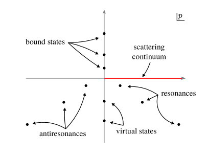
Figure 1: The analytic structure of the $S$ matrix indicating its poles in the $p$ plane corresponding to bound states, virtual states, resonances, and antiresonances (capturing resonances). Note especially how bound states lie on the positive imaginary axis while resonances are located in the 4 quadrant.

For bound states, the $S$-matrix $s_{l}(k)$ has corresponding poles on the positive imaginary axis, and it is customary to define the binding momentum $\kappa$ by writing $k=\mathrm{i}\kappa$, with $\kappa>0$. At such poles, bound-state wave functions are uniquely defined [faldt97_2542] by $\kappa$ and we can write

$$\psi_{l,k}(r)\xrightarrow[r\rightarrow\infty]{}N\,\hat{h}^{+}_{l}(\mathrm{i}\kappa r)\,,$$ (10)

which for an $S$-wave bound state reduces to

$$\psi_{0,k}(r)\xrightarrow[r\rightarrow\infty]{}N\,\exp({-}\kappa r)\,.$$ (11)

For all $l$ it is apparent from the behavior of the Riccati-Hankel functions for positive imaginary arguments that bound-state wave functions tend to zero exponentially for large $r$. If a bound state exists close to the scattering threshold, $k=0$, it follows from the analyticity of the partial-wave $S$ matrix as a function of $E\sim k^{2}$ that the scattering cross section gets enhanced at small $k$.

Resonances are another phenomenon that can cause enhancement of the scattering cross section. While the physically intuitive interpretation of resonances describes them as short-lived “metastable” states, formal scattering theory associates resonances with complex $S$-matrix poles, leading to an enhancement of the scattering cross section if they are located near the positive real axis (in either momentum or energy representation). These poles are known as “Gamow” or “Gamow-Siegert” states. It is clear that they are not ordinary eigenstates of the Hamiltonian $H=H_{0}+V$, which, as a Hermitian operator, can only have real eigenvalues. There is, however, a well-defined extension of scattering theory to incorporate resonances as eigenstates in a generalized sense by introducing the concept of so-called “rigged Hilbert spaces (RHSs).” In fact, already scattering states are not normalizable in the sense of possessing square-integrable wave functions, and therefore they do not reside within the ordinary Hilbert space. From this perspective, they should strictly be considered within the RHS framework. For practical applications, however, the mathematical complexity associated with this is rarely necessary and can be avoided by, for example, restricting the discussion to the radial Schrödinger equation and the properties of wave functions that solve this ordinary differential equation. In the same spirit, we can characterize decaying Gamow states as solutions of Eq. (6) that satisfy the asymptotic boundary condition specified in Eq. (9), albeit with a complex $k$ satisfying $\mathrm{Re}(k)>0$ and $\mathrm{Im}(k)<0$, i.e., located in the 4 quadrant of the complex-momentum plane.

II.2 $S$-matrix pole trajectories

If the potential supports a bound state, it is possible, as a theoretical exercise, to gradually weaken its strength to move the associated pole into the complex-momentum plane. The trajectory of the pole depends on the angular momentum of the state and the details of the potential. For example, the pole associated with an $S$-wave bound state generated by a purely attractive potential will simply move down the imaginary axis in the complex-momentum plane and become a virtual state after crossing through the $k=0$ threshold. In the complex-energy plane, the bound-state pole, located on the negative real axis, first moves towards the origin at $E=0$ and then moves backward as a virtual state on the second Riemann sheet of the $S$ matrix. The two sheets of the $S$ matrix as a function of $E$ are determined by the double-branched nature of the square-root function, $k=\pm\sqrt{2\mu E}$. The standard convention, which we also adopt here, is to attach the two sheets along the positive real axis, the so-called “unitarity cut.”

If instead the potential has a barrier, either from the actual shape of $V(r)$ or effectively due to the nonzero centrifugal term in Eq. (6) for $l>0$, the pole may also move through the threshold into the 4 quadrant (in both the momentum and the energy planes) so that the state becomes a (decaying) resonance. This is the scenario that is of primary interest to us in this work. In particular, in Sec. III.2 we develop a strategy to extrapolate along such a trajectory, as illustrated in Fig. 2.

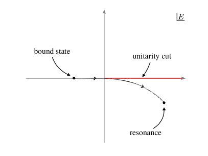
Figure 2: An illustration of a bound state moving through the complex-energy plane as the potential is made gradually weaker. In this case, it crosses the threshold and moves into the second Riemann sheet to become a resonance (Gamow state) with a complex energy.

II.3 Complex-scaling method (CSM)

As described above, bound states have associated imaginary momenta $k=\mathrm{i}\kappa$ with real $\kappa>0$, whereas resonances are described by complex $k$ with $\mathrm{Im}(k)<0$. This means that asymptotically, resonance wave functions grow exponentially with $r$ and are therefore—like scattering states but in some sense even more so—not square-integrable; i.e., they do not correspond to normalizable states in the ordinary Hilbert space. While the rigged Hilbert space construction offers a rigorous mathematical formalism to deal with this difficulty (see, for example, Ref. [delaMadrid:2012aa] for an introduction), for practical calculations there exists a much simpler alternative. The so-called (uniform) complex-scaling method [reinhardt82_708, Moiseyev:1998aa] enables a description of resonances with, essentially, bound-state techniques. This is achieved by expressing the wave function not as usual along the real $r$ axis, but on a contour rotated into the complex-$r$ plane. This can be achieved by applying the transformation

$$r\to re^{\mathrm{i}\phi}$$ (12)

to Eq. (6), with some angle $\phi$. The proper choice of $\phi$ in general depends on the position of the resonance one wishes to study. If the state of interest has a complex energy $E$, then it is necessary to ensure that $\phi>{-}\frac{\arg{E_{r}}}{2}$. As $E$ is usually not known beforehand, one might repeat the calculation while increasing $\phi$ until a resonance is found.

With the convention in Eq. (12), $r$ is still a real parameter but no longer describes the physical radial coordinate of the system. The overall argument $kre^{\mathrm{i}\phi}$ of the Riccati-Hankel function in Eq. (9) satisfies $\mathrm{Im}(kre^{\mathrm{i}\phi})>0$, and therefore square-integrability of the wave function as a function of $r$ is recovered. An example of such a scaled wave function is illustrated in Fig. 3.

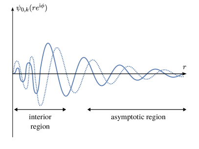
Figure 3: Illustration of the reduced radial wave function of a typical $S$-wave resonance (Gamow state), on a complex-scaled $r$ contour. The solid (dotted) line corresponds to the real (imaginary) part. It asymptotically converges to the Riccati-Hankel function $\hat{h}^{+}_{0}(kre^{\mathrm{i}\phi})=\hat{h}^{+}_{0}(\tilde{k}r)=\exp(\mathrm{i}\tilde{k}r)$, where we define $\tilde{k}=ke^{\mathrm{i}\phi}$, the effective wave number with $\mathrm{Im}(\tilde{k})>0$, so that it is normalizable just like bound-state wave functions.

It was shown in Ref. [Afnan:1991kb] that the scaling of the radial coordinate $r$ is equivalent to a rotation in momentum representation that goes in the opposite (clockwise) direction with the same angle $\phi$. That is, if we consider the wave function of the state as a function of a momentum coordinate $q$, then complex scaling is implemented via

$$q\to qe^{{-}\mathrm{i}\phi}\,.$$ (13)

This procedure then makes it possible to alternatively calculate resonance wave functions in momentum space. Note furthermore that scaling in momentum space can also be understood as a rotation of the branch cut in the complex-energy plane by an angle $2\phi$ clockwise, thereby exposing a section of the second Riemann sheet where resonances are located.

After this transformation, we can absorb the $e^{\mathrm{i}\phi}$ phase into the wave number $k$ and define the effective wave number as $\tilde{k}=ke^{\mathrm{i}\phi}$, so that the asymptotic form in Eq. (9) is preserved as

$$\psi_{l,k}(re^{\mathrm{i}\phi})\xrightarrow[r\rightarrow\infty]{}N\,\hat{h}^{+}_{l}(\tilde{k}r)\,.$$ (14)

The scaling technique can thus be interpreted as mapping resonances from the 4 quadrant in the complex-$k$ plane to the 1 quadrant in the $\tilde{k}$ plane (see Fig. 4). For future reference, we note that, at the same time, it will effectively map bound states from the positive imaginary $k$ axis to the 2 quadrant in the complex $\tilde{k}$ plane.

\begin{overpic}[width=212.47617pt]{rotation_a} \put(6.0,4.0){(a)} \end{overpic}

\begin{overpic}[width=212.47617pt]{rotation_b} \put(6.0,4.0){(b)} \end{overpic}

Figure 4: Trajectory of an $S$-matrix pole in the $k$ plane before (a) and after (b) complex scaling. Thanks to the CSM, resonance solutions have $\mathrm{Im}(\tilde{k})>0$ and thus are square-integrable. Also note how complex-scaled bound states come with “negative” wave numbers [$\mathrm{Re}(\tilde{k})<0$] while resonances come with “positive” wave numbers [$\mathrm{Re}(\tilde{k})>0$]. Indicated by asterisks are the CA-EC vectors discussed in Sec. III.2. They are obtained by complex conjugation of bound-state wave functions and will have asymptotic wave numbers ${-}\tilde{k}^{*}=\tilde{k}e^{{-}2\mathrm{i}\phi}$, placing them in the 1st quadrant and closer to the resonance regime.

II.4 Non-Hermiticity and the c-product

In traditional quantum mechanics, one requires the Hamiltonian $H$ to be Hermitian ($H^{\dagger}=H$) to ensure that the energy spectrum, being a physical observable, is real and that time evolution is strictly unitary, i.e., the norm of quantum states are preserved under the time evolution operator $\mathrm{e}^{{-}\mathrm{i}Ht/\hbar}$. However, when considering decay, an inherently time-dependent phenomenon, in a time-independent framework such as the complex-scaling method, the Hamiltonian is no longer Hermitian. Instead, in the present case, it becomes complex symmetric ($H^{T}=H$) [Moiseyev:1998aa]. This permits the energy spectrum to include complex eigenvalues, which, as discussed in Sec. II.1, is precisely what is needed to describe resonances. In fact, the non-Hermiticity and the corresponding nonunitary time evolution of Gamow states are well aligned with the physical interpretation of resonances as metastable systems that ultimately decay.

Similarly to how nondegenerate eigenvectors of a Hermitian operator are orthogonal under the inner product defined on the Hilbert space, the nondegenerate eigenvectors of a complex symmetric operator are orthogonal under the so-called “c-product” [Moiseyev:1978aa, Moiseyev:2011]. For eigenstates $\ket{\psi_{1}}$ and $\ket{\psi_{2}}$ with equal angular-momentum quantum numbers $(l,m)$, we define the c-product in coordinate representation as

$$\braket{\psi_{1}}{\psi_{2}}=\int\mathrm{d}r\,\psi_{1}(r)\psi_{2}(r)\,,$$ (15)

and similarly in momentum space. Note that $\psi_{1}(r)$ appears without complex conjugation under the integral. This is precisely the c-product introduced in Ref. [Moiseyev:1978aa] with the notation $(\psi_{1}|\psi_{2})$. In this paper, we use the standard notation $\braket{\psi_{1}}{\psi_{2}}$ with the implicit understanding that for complex-scaled systems this is meant to denote the c-product.

Equivalently, one can change the definition of bra states so that no complex conjugation is involved when they are associated with a complex-scaled system. This is so even for bound states calculated with complex scaling. Although the energies of such states remain real, wave functions become complex when defined along the rotated contour and the orthogonality of states with different binding energies is ensured only if no complex conjugation is performed for bras, leading again to the c-product [Moiseyev:2011]. Ultimately, these concepts can be understood by properly distinguishing bra and ket states as, respectively, left and right eigenvectors of the non-Hermitian complex-scaled Hamiltonian [Afnan:1991kb]. Even more rigorously, a comprehensive theory for Gamow bras and kets can be developed within the RHS formalism mentioned previously [delaMadrid:2012aa]. However, in practice we find it convenient and sufficient to employ complex scaling along with the c-product.

III Resonance continuation

We now discuss the extension of eigenvector continuation to resonance states. Generally, EC works by obtaining eigenstates of a Hamiltonian $H(c)$ with a parametric dependence on a parameter $c$ for several values of that parameter. The set of parameters $\{c_{i}\}$ used for this step is referred to as “training points,” and the corresponding “training vectors” $\ket{\psi(c_{i})}$ are used to construct an effective basis within which the problem is subsequently solved for one or more target values of the parameter $c$. For typical applications of EC, this procedure reduces the dimension of the problem from a large Hilbert space to the small subspace spanned by the training vectors, thereby leading to a vast reduction of the computational cost for each target evaluation. Specifically, if we denote the target point as $c_{*}$, EC involves solving the generalized eigenvalue problem

$$H_{\text{EC}}\ket{\psi(c_{*})}_{\text{EC}}=E(c_{*})_{\text{EC}}\,N_{\text{EC}}\ket{\psi(c_{*})}_{\text{EC}}\,,$$ (16)

with the following Hamiltonian and norm matrices:

$$\big{(}H_{\text{EC}}\big{)}_{ij} =\braket{\psi(c_{i})}{H(c_{*})}{\psi(c_{j})}\,,$$ (17)

$$\big{(}N_{\text{EC}}\big{)}_{ij} =\braket{\psi(c_{i})}{\psi(c_{j})}\,.$$ (18)

The key to making this remarkably simple prescription useful is that typically EC is able to construct highly effective variational bases, with rapid convergence as the number of training data is increased [Sarkar:2020mad].

Eigenvector continuation involving resonance states can be defined by prescribing that the matrix elements in Eqs. (17) and (18) are to be evaluated using the c-product. Importantly, this is to be used in connection with the complex-scaling technique described in Sec. II.3, so that for evaluating the c-product one integrates along the rotated contour in either $r$ space or $q$ space. This procedure ensures in particular that all matrix elements remain well defined and finite, which would not be the case without complex scaling because, as previously mentioned, Gamow states would then not be normalizable and their wave functions would exhibit, in coordinate representation, an exponentially growing amplitude. The Hamiltonian and norm matrices, $H_{\text{EC}}$ and $N_{\text{EC}}$, obtained with the c-product will not be Hermitian but complex symmetric, and therefore they may have complex eigenvalues, as is required to describe resonances.

Numerical tests.

We can show with explicit examples that indeed this procedure works nicely in practice. All of the calculations shown in the following sections were performed using a discrete momentum basis with a cutoff of $\Lambda=8.0$ (in the dimensionless units explained above) and consisting of $N=256$ mesh points distributed according to a 256-point Gauss–Legendre quadrature to ensure convergence. In general, the proper choice of $\Lambda$ and $N$ depends on the properties of $V$, and we have checked that the above is sufficient to ensure numerical convergence for the particular examples we describe below. Furthermore, the momentum basis is complex-scaled as discussed previously, by an angle $\phi=\pi/6$. As a crude way to estimate the uncertainty of the EC extrapolations, we repeat every calculation $128$ times while randomizing the training points within the given interval. Finally, the distributions of the extrapolation results are indicated in figures by their $68.2\%$ and $95.4\%$ percentile intervals, the approximate intervals corresponding to 1 and 2 standard deviations, respectively.

All of the potentials we use for numerical tests are based on a local Gaussian form, which in configuration space reads

$$F(\alpha,r)=\exp\left(-\alpha r^{2}\right)\,.$$ (19)

For momentum-space calculations, we take the Hankel transform of the above. This is given by

$$F_{l}(\alpha,q,q^{\prime})=\frac{2}{\pi}\int_{0}^{\infty}\mathrm{d}r\,\hat{j}_{l}(qr)\exp\left(-\alpha r^{2}\right)\hat{j}_{l}(q^{\prime}r)\,,$$ (20)

where $\hat{j}_{l}(z)$ are the Riccati-Bessel functions (see Ref. [Taylor:1972pty, p. 182]). For $l=0$, this reduces to

$$F_{0}(\alpha,q,q^{\prime})=\frac{1}{\sqrt{\alpha\pi}}\exp\left(-\frac{q^{2}+q^{\prime 2}}{4\alpha}\right)\sinh\left(\frac{qq^{\prime}}{2\alpha}\right)\,.$$ (21)

For $l=1$, we have F_1(α,q,q’)=α4π [ (1α+2q q’) exp(-(q+q’)24α)
+ (1α-2q q’) exp(-(q-q’)24α) ]  . Because there is no centrifugal term in the $S$-wave radial equation, we include in the $l=0$ potential a repulsive barrier to support resonances:

$$V(c,q,q^{\prime})=c\left[-5F_{0}\left(\nicefrac{{1}}{{3}},q,q^{\prime}\right)+2F_{0}\left(\nicefrac{{1}}{{10}},q,q^{\prime}\right)\right]\,.$$ (22)

For a $P$-wave example, the following simple Gaussian potential is considered:

$$V(c,q,q^{\prime})=-cF_{1}\left(\nicefrac{{1}}{{4}},q,q^{\prime}\right)\,.$$ (23)

Although not exploited here, we note that Hamiltonians $H(c)$ with a simple linear dependence on $c$ (like the ones we consider), or more generally, an affine dependence on a vector of parameters $\mathbf{c}$, permit further optimization of the EC calculation via decomposition into off-line and on-line tasks, see for example Ref. [Drischler:2022ipa].

As Supplemental Material, we provide the code for our calculations as downloadable files [supp]. The setup is split into a python library, twobodyEC.py, that implements the basic numerical techniques discussed above, and a jupyter notebook, calculations.ipynb, that reproduces the exact numerical examples presented in the following.

III.1 Resonance-to-resonance extrapolation

We now consider a Hamiltonian $H(c)$ that supports a resonance for some range of $c$ and we implement the standard EC prescription by first constructing $H(c_{i})$ on a complex-scaled basis for several training points $\{c_{i}\}$. In our calculation, this amounts to calculating the matrix elements $\braket{q_{n}e^{{-}\mathrm{i}\phi}}{H(c_{i})}{q_{m}e^{{-}\mathrm{i}\phi}}$ using a $q$ momentum mesh as described previously (with $\phi>{-}\frac{\arg{E_{r}}}{2}$, where $E_{r}$ is the complex energy associated with the resonance for all $c$ within the region of interest). Then we proceed to solve the system to obtain the exact eigenvectors $\ket{\psi(c_{i})}$ for each $c_{i}$. This is the part that takes the bulk of the computational time.

We now want to determine $E(c_{*})$ at some target point $c=c_{*}$ via extrapolation. To that end, we construct $H(c_{*})$, but instead of determining its eigenvalues directly, we project $H(c_{*})$ onto the “EC subspace” spanned by $\{\ket{\psi(c_{i})}\}$. In practice, this is done by calculating the projected matrix elements $(H_{\text{EC}})_{i,j}=\braket{\psi(c_{i})}{H(c_{*})}{\psi(c_{j})}$ and the norm matrix elements $(N_{\text{EC}})_{i,j}=\braket{\psi(c_{i})}{\psi(c_{j})}$. The latter accounts for the nonorthogonality of the basis vectors. The c-product prescription has to be followed in this step. Finally, we diagonalize the much smaller projected matrix $H_{\text{EC}}$ by solving the generalized eigenvalue problem

$$H_{\text{EC}}\,\ket{\psi(c_{*})}_{\text{EC}}=E(c_{*})_{\text{EC}}\,N_{\text{EC}}\,\ket{\psi(c_{*})}_{\text{EC}}\,.$$ (24)

Equation (24) yields a spectrum of complex eigenvalues that includes the approximation $E(c_{*})_{\text{EC}}$ corresponding to the exact energy eigenvalue $E(c_{*})$ of the particular state we are interested in. Identification of the relevant $E(c_{*})_{\text{EC}}$ for non-Hermitian systems cannot be based on the variational principle, and so, unlike EC applied to bound states, it is not sufficient here to simply pick extremal eigenvalues from the EC spectrum. Because for the benchmark presented here the exact value $E(c_{*})$ is calculated alongside the extrapolated spectrum, we employ the criterion $\min|E(c_{*})_{\text{EC}}-E(c_{*})|$ to identify the proper state within the complex spectrum. For practical applications of the technique, the exact $E(c_{*})$ will typically be unknown. To deal with this situation, one might manually follow the extrapolated pole as it gradually crosses the threshold from being a bound state (for which the identification is straightforward) to becoming a resonance. More generally, one may employ a systematic overlap-based technique as is common practice in the calculation of resonances within the Berggren basis [michel03_10].

To exemplify resonance-to-resonance continuation, the system described by Eq. (22) is considered. Results are shown in Fig. 5.

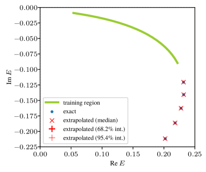
Figure 5: Application of EC for resonance-to-resonance extrapolation. Five training points were randomly drawn from the region $c\in(0.45,0.78)$ per dataset. Apart from using the c-product formalism, the calculation proceeds similar to ordinary EC, yielding accurate approximations for the complex-energy eigenvalues of resonances (Gamow states). See text for details.

III.2 Bound-state-to-resonance extrapolation

While applying EC solely within the resonant regime is interesting and certainly useful in practice (e.g. to produce EC-based emulators for uncertainty quantification [Konig:2019adq]), it is a more fascinating question whether we can set up an extrapolation scheme that uses training vectors at $c$ values corresponding only to bound states, but which then extrapolates to $c_{*}$ where the state is a resonance. In other words, we would like to use EC to extrapolate along the $S$-matrix pole trajectories described in Sec. II.2 from the regime of bound states into the resonance domain. We note that, in general, not all bound states transition into resonances as illustrated in Sec. II.2, but in order to illustrate the method we consider here only cases where it is known a priori that this is the case.

Clearly, a naive approach without appropriate complex scaling of the basis will not be successful in predicting resonance energies because $H_{\text{EC}}$ and $N_{\text{EC}}$ will be trivially Hermitian with that prescription. However, even with complex scaling and the matrix elements defined in terms of the c-product, it is not possible to obtain complex energies via EC because $H_{\text{EC}}$ and $N_{\text{EC}}$ will, in fact, be real and symmetric. This can be seen as follows. If we use the notation $\psi(c_{i};r)$ for the (reduced) radial wave function corresponding to the state $\ket{\psi(c_{i})}$, then for the norm matrix it holds that (N_EC)_ij &=⟨ψ(c_i) — ψ(c_j)⟩
=∫_C dr   ψ(c_i;r) ψ(c_j;r)
=∫_0^∞dr   ψ(c_i;r) ψ(c_j;r) ∈R , where $\int_{C}$ denotes integration along the complex-scaled contour. We have used the fact that the contour can be rotated back to the real axis without changing the value of the integral because no singularities are swept over and for bound states the contribution of the arc at infinity that closes the curve between the real axis and the rotated contour vanishes. Then, we have made use of the fact that “c-normalized” bound-state wave functions are real along the real axis. This is so because any bound-state wave function $\varphi(r)$ can be chosen to be real and any arbitrary global factor $N$ will be constrained to $N\in\mathbb{R}$ by the c-normalization condition

$$\int_{0}^{\infty}\mathrm{d}r\,\left[N\varphi(r)\right]^{2}=1\,,$$ (25)

resulting in a real normalized wave function $\psi(r)=N\varphi(r)$. $N_{\text{EC}}$ is also trivially symmetric due to the properties of the c-product.

By the same token, for the projected Hamiltonian matrix, we see that (H_EC)_ij &=⟨ψ(c_i) —H(c_*) — ψ(c_j)⟩
=∫_C dr ∫_C dr’   ψ(c_i;r) H(c_*;r,r’) ψ(c_j;r’)
=∫_0^∞dr ∫_0^∞dr’   ψ(c_i;r) H(c_*;r,r’) ψ(c_j;r’)
∈R , noting that everything under the final integral is real. This shows that $H_{\text{EC}}$ has only real entries. Because $H(c_{*})$ is complex only due to the contour rotation, by the “turn over rule” [Moiseyev:1998aa] it follows moreover that $H_{\text{EC}}$ is symmetric, which concludes the proof.

The same $S$-wave potential given in Eq. (22) is considered for demonstrating the failure of a naive bound-state-to-resonance extrapolation. As shown in Fig. 6, the extrapolated energies do not extend beyond the real axis, as one would expect for resonance states.

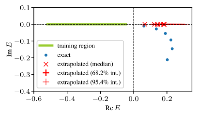
Figure 6: Attempt to extrapolate from bound states to resonances using ordinary EC without augmentation. Five training points were randomly drawn from the region $c\in(0.9,1.3)$ per dataset. See text for details.

Conjugate-augmented EC.

Fortunately, it turns out that there is a way to accomplish bound-state-to-resonance extrapolations with an extension of the EC prescription. The appropriate strategy, which we refer to as “conjugate-augmented eigenvector continuation (CA-EC)” and which we elucidate further below, is to enlarge the subspace spanned by the bound-state training vectors by including, in addition, complex-conjugate versions of the existing wave functions. This can be easily implemented numerically (in any concrete representation of the wave functions) by duplicating training vectors stored in memory with elementwise complex conjugation.

As we show with concrete examples below, CA-EC works nicely in practice. To understand why that is so, note that after complex scaling the asymptotic wave functions (as functions of $r$ along the rotated contour) will have decaying wave numbers for both bound states and resonances, i.e., $\mathrm{Im}(\tilde{k})>0$, as illustrated in Fig. 4. However, $\mathrm{Re}(\tilde{k})$ is negative for bound states and positive for resonances. EC is ineffective at extrapolating complex “plane waves” of the form $\hat{h}^{+}_{l}(\tilde{k}r)$ with rapidly changing wave numbers, especially when the sign of the real part is supposed to change upon extrapolating from the training regime to the target point. This systematic deficiency of the basis can be remedied by including additional vectors that have “positive” asymptotic wave numbers, i.e., $\mathrm{Re}(\tilde{k})>0$. Exactly this is achieved with CA-EC because the complex-conjugated wave functions have such asymptotic wave numbers. Specifically, the asymptotic wave number of a complex-conjugated bound state will be ${-}\tilde{k}^{*}=\tilde{k}e^{{-}2\mathrm{i}\phi}$ if $\tilde{k}$ denotes the wave number of the bound state (cf. Fig. 4).

The systems described by Eqs. (22) and (23) are considered to illustrate the CA-EC bound-state-to-resonance extrapolation method. As shown in Figs. 7 and 8, CA-EC can reproduce resonance states, and the extrapolated energies agree nicely with exact calculations performed for comparison.

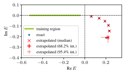
Figure 7: Bound-state-to-resonance extrapolation performed with CA-EC for the system given by Eq. (22). Five training points were randomly drawn from the region $c\in(0.9,1.3)$ per dataset. See text for details.

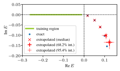
Figure 8: Bound-state-to-resonance extrapolation with CA-EC for the Gaussian potential shown in Eq. (23) in the $P$ wave. Five training points were randomly drawn from the region $c\in(3.1,4.0)$ per dataset. See text for details.

The key to understanding why CA-EC works is the insight that in the interior region (i.e., $r$ sufficiently small), resonance wave functions look similar to those of bound states. As shown in Fig. 3, the oscillating and exponentially growing behavior only sets in at larger $r$. Therefore, in the interior region, an EC basis comprised of bound states can properly express the behavior of the resonance wave function at the target point, and it is only the asymptotic behavior that needs an enlarged basis to be properly represented. To further elucidate this explanation, we can consider an alternative approach where we augment the original EC basis not with complex-conjugated versions of the training bound-state wave functions, but with Riccati-Hankel functions $\hat{h}^{+}_{l}(\tilde{k}r)$ that have the same wave numbers $\tilde{k}$ that are otherwise provided by the complex-conjugated bound states with CA-EC (i.e. asterisks in Fig. 4). This approach is somewhat similar to the construction of the so-called Berggren basis [Berggren:1968zz, Berggren:1993zz].

This basis augmentation with Riccati-Hankel functions can be performed in configuration space as well as in momentum space. In configuration space, we can use the explicit representation [DLMF, Eq. 10.49.6]

$$\hat{h}^{+}_{l}(kr)=\exp(\mathrm{i}kr)\sum_{n=0}^{l}{\frac{\mathrm{i}^{n-l-1}}{2^{n}}\frac{(l+n)!}{n!(l-n)!}\frac{1}{(kr)^{n}}}\,,$$ (26)

for a state with angular momentum $l$. In momentum space, we need the Hankel transform of $\hat{h}^{+}_{l}(kr)$, which is given by

$$\phi_{k}(q)=\sqrt{\frac{2}{\pi}}\frac{k\left(q/k\right)^{l}}{q^{2}-k^{2}}\,.$$ (27)

This can be verified by explicitly carrying out the inverse Hankel transform as follows: 2π∫_0^∞dq   ^j_l(qr)