Full State Estimation of Continuum Robots From Tip Velocities: A Cosserat-Theoretic Boundary Observer

Abstract

State estimation of robotic systems is essential to implementing feedback controllers which usually provide better robustness to modeling uncertainties than open-loop controllers. However, state estimation of soft robots is very challenging because soft robots have theoretically infinite degrees of freedom while existing sensors only provide a limited number of discrete measurements. In this paper, we design an observer for soft continuum robotic arms based on the well-known Cosserat rod theory which models continuum robotic arms by nonlinear partial differential equations (PDEs). The observer is able to estimate all the continuum (infinite-dimensional) robot states (poses, strains, and velocities) by only sensing the tip velocity of the continuum robot (and hence it is called a “boundary” observer). More importantly, the estimation error dynamics is formally proven to be locally input-to-state stable. The key idea is to inject sequential tip velocity measurements into the observer in a way that dissipates the energy of the estimation errors through the boundary. Furthermore, this boundary observer can be implemented by simply changing a boundary condition in any numerical solvers of Cosserat rod models. Extensive numerical studies are included and suggest that the domain of attraction is large and the observer is robust to uncertainties of tip velocity measurements and model parameters.

Continuum robots, soft robots, boundary estimation, Cosserat rod theory, PDE systems

1 Introduction

Soft robotics is a rapidly growing research area [1]. Thanks to their compliant property, soft robots are safer when interacting with humans and are adaptable in constrained environments. As a result, soft robots have found many applications such as medical surgeries and underwater maneuvers [2].

Despite the empirical success, the theoretical study of soft robots has been considered a challenging problem. In May 2023, the IEEE Control Systems Magazine published a special issue that highlights the control challenges for soft robotics [3]. Over the past years, theoretical and experimental studies have suggested that feedback schemes are more robust to modeling uncertainties of soft robots [4]. Nevertheless, perception of soft robots is also a challenging task because theoretically, soft robots have infinite degrees of freedom, while existing sensors can only provide a limited number of discrete measurements of the continuum states. Moreover, some robot states (like strains) are more difficult to measure than others (like positions). This work is thus devoted to designing algorithms to estimate the unknown states from sensor measurements.

The majority of existing work has focused on static estimation (or shape estimation), which assumes that the robot is in a quasi-static state and aims to estimate the configuration of the entire continuum robot from discrete measurements of certain variables, such as position and orientation. The common strategy is to fit a parametrized static (time-independent) spatial curve to the discrete measurements [5, 6]. The accuracy of this approach depends on the complexity of the assumed curve model and the number of discrete measurements. Physically more plausible solutions are those that fit a mechanical equilibrium (represented by ordinary differential equations of the arc parameter) to the discrete measurements along the arc length, such as a static Kirchhoff rod [7] or a static Cosserat rod [8].

Due to the quasi-static assumption, the above-mentioned static estimation methods have server limitations, such as the restriction to slow-speed motions. Hence, the recent trend is to design a dynamic state estimator. Dynamic estimation (or state estimation) is an iterative process that uses a dynamic system model and its inputs to predict new states and uses sequential sensor measurements to correct the prediction. The most widely adopted dynamic models of continuum robots include geometrical models and continuum mechanics models [9, 4]. Geometrical models (especially the piecewise constant curvature models) represent the continuum robot using a finite number of basis functions [10, 11]. Continuum mechanics models (especially the Cosserat rod models) benefit from a physically rigorous definition of the kinetic and potential energy of the system and usually take forms of nonlinear PDEs [12, 13, 14, 15] which are very difficult to study. Therefore the majority of existing work on dynamic estimation relies on some form of finite-dimensional approximation, such as finite-dimensional Lagrangian [16, 17] or port-Hamiltonian representations [18]. Relying on some of these discretized dynamic models, extended Kalman filters (EKFs) have been applied for state estimation of continuum robots [19, 20]. Nevertheless, state estimation based on the original continuum mechanics PDEs has rarely been explored. To the best of our knowledge, the only existing work is our previous work [21] where a PDE-based EKF is reported.

In summary, existing work has revealed several limitations. First, existing work has mainly relied on finite-dimensional approximations, which may introduce extra modeling uncertainty. Second, existing work typically requires a large number of sensors for good accuracy, which can be expensive and also damage the compliant property of soft robots. Third, no result is available concerning the convergence of estimation errors. This work is motivated to address these limitations.

In this work, we design a boundary observer for continuum robotic arms based on the well-known Cosserat rod theory [12, 13, 14, 15] and prove its (local) stability. This boundary observer is able to estimate all the infinite-dimensional robot states, e.g., poses, strains, and velocities, using the PDE model, inputs, and only tip velocity measurements (which explains the name “boundary” observer). The key idea is to inject sequential tip velocity measurements into the observer in a way that dissipates the energy of state estimation errors through the boundary. It has three major advantages over the existing work.

1. It only requires sensing the tip velocity.

2. It can be implemented by changing a boundary condition in existing numerical solvers for Cosserat rod models.

3. The state estimation error is proven to be locally input-to-state stable.

This is the first work that is able to construct a (locally) stable PDE-based observer for continuum robots. To highlight its contribution, we point out that stability guarantees for nonlinear state estimation are difficult even for finite-dimensional systems. Boundary estimation of PDEs is even harder because one needs to estimate infinite-dimensional continuum states from only point measurements at the boundary. The Cosserat rod PDE studied in this work is a semilinear hyperbolic system formulated on the Lie algebra of the Lie group $SE(3)$ [22]. While boundary estimation of certain general classes of hyperbolic PDEs has been studied before [23, 24], their assumptions (of linearity or global Lipschitz continuity of the nonlinear terms) are not satisfied by the Cosserat rod PDE. The Lie group structure also poses additional difficulties to state estimation because the system states of the Cosserat rod PDE are defined in the local body frames while the effect of certain inputs (like gravity) is expressed in the global world frame. In this regard, the (local) stability guarantee provided in this work is also a novel contribution in the context of boundary estimation of PDE systems. Numerical studies using SoRoSim [25], a MATLAB toolbox for soft robots, suggest that the domain of attraction is large and the observer is robust to uncertainties of tip measurements and model parameters. The results in this work suggest the promising role of PDE control theory in the theoretical study of soft robots.

The rest of the paper is organized as follows. In Section 2, we introduce the Cosserat rod model and the state estimation problem. In Section 3, we design a boundary observer and prove its stability. In Section 4, we conduct a series of numerical experiments to validate the performance and robustness of the boundary observer. Section 5 summarizes the contribution and points out future direction.

2 Modeling and Problem Formulation

2.1 Notations and Preliminaries

We will make use of some Lie group notations from [22]. Denote by $SO(3)$ the special orthogonal group (the group consisting of 3D rotations) and by $so(3)$ its associated Lie algebra. Denote by $SE(3)=SO(3)\times\mathbb{R}^{3}$ the special Euclidean group (the group consisting of 3D poses) and by $se(3)$ its associated Lie algebra. A hat $\wedge$ at the superscript of a vector $\eta$ defines a matrix $\eta^{\wedge}$ whose definition depends on the dimension of $\eta$. Specifically, if $\eta\in\mathbb{R}^{3}$, then $\eta^{\wedge}\in so(3)$ is such that $\eta^{\wedge}\xi=\eta\times\xi$ for any $\xi\in\mathbb{R}^{3}$ where $\times$ is the cross product. If $\eta=[w^{T},v^{T}]^{T}\in\mathbb{R}^{6}$ with $w,v\in\mathbb{R}^{3}$, then $\eta^{\wedge}\in se(3)$ is defined by

$$\eta^{\wedge}=\begin{bmatrix}w^{\wedge}&v\\ 0&0\end{bmatrix}\in\mathbb{R}^{4\times 4}.$$

Let the superscript $\vee$ be the inverse operator of $\wedge$, i.e., $(\eta^{\wedge})^{\vee}=\eta$. The adjoint operator $ad$ of $\eta=[w^{T}~{}v^{T}]^{T}\in\mathbb{R}^{6}$ with $w,v\in\mathbb{R}^{3}$ is defined by

$$ad_{\eta}=\begin{bmatrix}w^{\wedge}&0\\ v^{\wedge}&w^{\wedge}\end{bmatrix}\in\mathbb{R}^{6\times 6}.$$

By definition, $ad$ is a linear operator and satisfies $ad_{\eta}\xi=-ad_{\xi}\eta$ for $\xi,\eta\in\mathbb{R}^{6}$. The Adjoint operator of any element $g=(R,p)\in SE(3)$ with $R\in SO(3),p\in\mathbb{R}^{3}$ is defined by

$$Ad_{g}=\begin{bmatrix}R&0\\ p^{\wedge}R&R\end{bmatrix}\in\mathbb{R}^{6\times 6}.$$

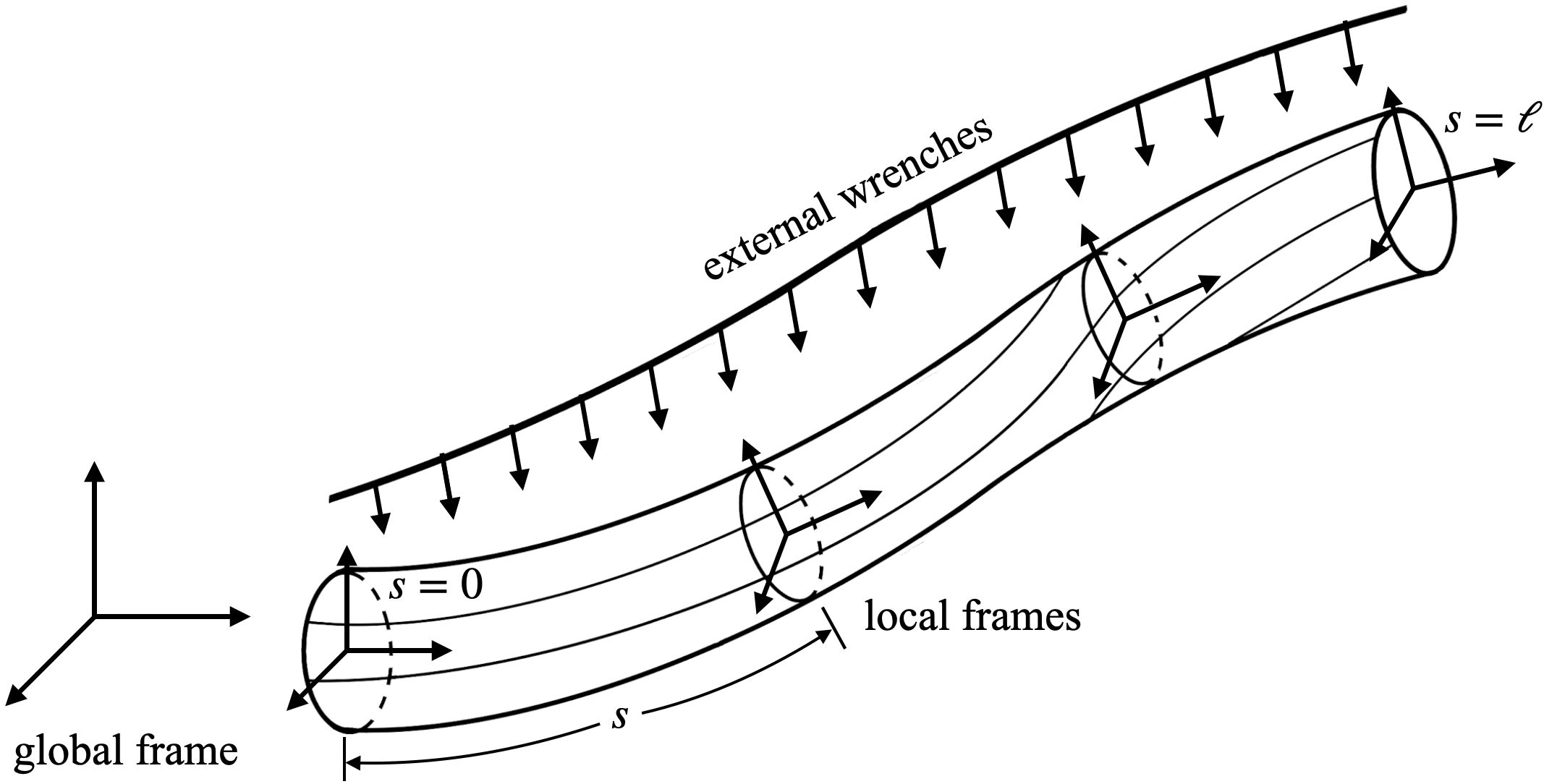
Figure 1: A Cosserat rod.

2.2 Cosserat Rod Models For Continuum Robots

Cosserat rod models are continuum mechanics models that describe the dynamic response of long and thin deformable rods undergoing external wrenches and have been widely used to model continuum robots [13, 14, 15, 26].

2.2.1 Configuration

A Cosserat rod is idealized as a continuous set of rigid cross-sections stacked along a centerline parameterized by the arc parameter $s\in[0,\ell]$; see Fig. 1. Let $t\in[0,T]$ be time. The pose of the entire rod is uniquely defined by a function $g(s,t)\in SE(3)$ given by

$$g=\begin{bmatrix}R&p\\ 0&1\end{bmatrix},$$

where $p(s,t)\in\mathbb{R}^{3}$ is the position vector of the centerline and $R(s,t)\in SO(3)$ is the rotation matrix of the cross-sections. Note that there is a unique global world frame while each cross-section also defines a local body frame.

2.2.2 Kinematics

Let $w(s,t),v(s,t),u(s,t),q(s,t)\in\mathbb{R}^{3}$ be the fields of the angular velocity, linear velocity, angular strain, and linear strain, respectively, of the cross-sections in their local frames. Let $\eta=[w^{T}~{}v^{T}]^{T}$ and $\xi=[u^{T}~{}q^{T}]^{T}$ be the fields of velocity twists and strain twists, respectively. The kinematics of the Cosserat rod is given by

$$\partial_{t}g=g\eta^{\wedge},$$ (1)

$$\partial_{s}g=g\xi^{\wedge},$$ (2)

where $\partial_{t}:=\frac{\partial}{\partial t}$ and $\partial_{s}:=\frac{\partial}{\partial s}$ are partial derivatives. The equality of mixed partial derivatives $\partial_{st}g=\partial_{ts}g$ yields the compatibility equation between the strain and the velocity

$$\partial_{t}\xi=\partial_{s}\eta+ad_{\xi}\eta.$$ (3)

2.2.3 Dynamics

Let $m(s,t),n(s,t),l(s,t),f(s,t)\in\mathbb{R}^{3}$ be the fields of the internal moment, internal force, external moment, and external force, respectively, of the cross-sections in their local frames. Let $\Phi=[m^{T}~{}n^{T}]^{T}$ and $\Psi=[l^{T}~{}f^{T}]^{T}$ be the fields of internal and external wrenches, respectively. Applying Hamilton’s principle in the context of Lie groups yields the following dynamics of the Cosserat rod in the form of nonlinear PDEs

$$J\partial_{t}\eta-ad_{\eta}^{T}J\eta=\partial_{s}\Phi-ad_{\xi}^{T}\Phi+\Psi,$$ (4)

where $J(s)\in\mathbb{R}^{6\times 6}$ is the cross-sectional inertial matrix. We allow $J(s)$ to be a function of $s$ to account for, e.g., nonuniform cross-sectional areas. Since this work is primarily interested in continuum robotic arms, the following boundary conditions at $s=0$ and $s=\ell$ are adopted

$$\eta(0,t)=\eta_{-}(t),\quad\Phi(\ell,t)=\Psi_{+}(t),$$ (5)

where $\eta_{-}(t)$ is the velocity of the station to which the continuum robot is attached and $\Psi_{+}(t)$ is the point wrench applied at the tip.

2.2.4 Inputs

The inputs of continuum robots can arise in various forms. For generality, we assume

$$\Phi(s,t) =\phi(s,t)+\phi_{\text{loc}}(s,t),$$ (6)

$$\Psi(s,t) =\psi_{\text{loc}}(s,t)+Ad_{g(s,t)}^{-1}\psi_{\text{glb}}(s,t),$$ (7)

$$\Psi_{+}(t) =\psi_{\text{loc}}^{+}(t)+Ad_{g(\ell,t)}^{-1}\psi_{\text{glb}}^{+}(t).$$ (8)

In (6), $\phi_{\text{loc}}$ represents the distributed wrench (force and moment) applied internally with respect to the local frames (like pneumatic or tendon actuation [27]) and $\phi$ is the field of wrench due to elastic deformation and is assumed to satisfy the following linear constitutive law

$$\phi=K(\xi-\xi_{*}),$$ (9)

where $K(s)\in\mathbb{R}^{6\times 6}$ is the cross-sectional stiffness matrix and $\xi_{*}(s)$ is the strain field of the (undeformed) reference configuration. Again, $K(s)$ is allowed to be a function of $s$ to account for nonuniform material properties. In (7), $\psi_{\text{loc}}$ represents the distributed wrench applied externally whose value is specified in the local frames, and $Ad_{g}^{-1}\psi_{\text{glb}}$ represents the distributed wrench applied externally whose value is specified by $\psi_{\text{glb}}$ in the global world frame (like gravity and loads) and converted into the local frames through the coordinate transformation $Ad_{g}^{-1}$. It is important to distinguish between $\psi_{\text{loc}}$ and $Ad_{g}^{-1}\psi_{\text{glb}}$ for state estimation problems because the pose $g$ is also an unknown robot state. For simplicity, we assume $\psi_{\text{glb}}$ only consists of distributed forces, which holds true in most cases of manipulation problems. Thus, we have

$$\psi_{\text{glb}}=\begin{bmatrix}0\\ f_{\text{glb}}\end{bmatrix},\quad Ad_{g}^{-1}\psi_{\text{glb}}=\begin{bmatrix}0\\ R^{T}f_{\text{glb}}\end{bmatrix},$$ (10)

where $f_{\text{glb}}\in\mathbb{R}^{3}$ is the externally applied distributed force in the global world frame (like gravity). Similarly, in (8), $\psi_{\text{loc}}^{+}(t)$ represents the point wrench applied at the tip whose value is specified in the local frame and $Ad_{g(\ell,t)}^{-1}\psi_{\text{glb}}^{+}(t)$ represents the point wrench applied at the tip whose value is specified in the global world frame by $\psi_{\text{glb}}^{+}(t)$ (like a load attached at the tip).

Remark 1

A linear constitutive law with damping may be used to replace (9) by

$$\phi=K(\xi-\xi_{*})+D\partial_{t}\xi,$$ (11)

where $D\in\mathbb{R}^{6\times 6}$ is the damping matrix that models the viscoelastic property of the material. Our numerical study shows that the boundary observer to be presented later performs well in this case. From a theoretical perspective, however, (11) introduces mixed partial derivatives into the final PDE system, which makes it much harder to study its stability. More generally, nonlinear constitutive laws may also be used to replace (9), which will make the final PDE system quasilinear instead of semilinear. The extension to these general constitutive laws is left as future work. All the theoretical results in this work are based on assuming the linear constitutive law (9) which is known to be a good agreement for small strains, i.e., lower than 50% [28].

2.3 Formulation of the Estimation Problem

A minimum representation of the Cosserat rod model only requires two variables from the collection $\{g,\eta,\xi,\phi\}$ since the others can be correspondingly determined using (2) and (9) (or (11)). In our previous work [21], we chose $\{g,\eta\}$ and reported a PDE-based EKF. In this work, we mainly work with $\{\xi,\eta\}$ which satisfy the following semilinear hyperbolic system

$$\left\{\begin{aligned} &\partial_{t}\xi=\partial_{s}\eta+ad_{\xi}\eta,\\ &J\partial_{t}\eta=\partial_{s}(\phi+\phi_{\text{loc}})-ad_{\xi}^{T}(\phi+\phi_{\text{loc}})\\ &\qquad\quad+ad_{\eta}^{T}J\eta+\psi_{\text{loc}}+Ad_{g}^{-1}\psi_{\text{glb}},\\ &\begin{aligned} &(\phi+\phi_{\text{loc}})(\ell,t)=\psi_{\text{loc}}^{+}(t)+Ad_{g(\ell,t)}^{-1}\psi_{\text{glb}}^{+}(t),\\ &\eta(0,t)=\eta_{-}(t),\\ &\phi(s,0)=\phi_{0}(s),\\ &\eta(s,0)=\eta_{0}(s),\end{aligned}\end{aligned}\right.$$ (12)

where $g$ and $\phi$ are determined by (2) and (9) (or (11)) respectively at every $t$, and $\{\eta_{0},\phi_{0}\}$ are the initial conditions.

Assume the robot model (12), its left-boundary condition $\eta_{-}$, all the distributed inputs $\{\phi_{\text{loc}},\psi_{\text{loc}},\psi_{\text{glb}}\}$, and all the right-boundary inputs $\{\psi_{\text{loc}}^{+},\psi_{\text{glb}}^{+}\}$ are known. (The initial conditions are unknown.) Also assume that we can measure the tip velocity $\eta(\ell,t)$. This is called a boundary output/measurement and can be obtained by installing an initial measure unit (IMU) sensor at the tip. Note that once the tip velocity $\eta(\ell,t)$ is known, one can actually compute the tip pose $g(\ell,t)$. This is the classical pose estimation problem that has been extensively studied especially in the community of quadrotors and there exist efficient algorithms for this purpose, such as the complementary filter given in [29]. Thus, we will assume the tip pose $g(\ell,t)$ is also provided for simplicity. (In fact, this assumption is needed only when $\psi_{\text{glb}}^{+}$ is nonzero.) As a result, we essentially assume that the right-boundary condition $\Psi^{+}$ is known. Our objective is to estimate the continuum robot states $\{\xi,\eta\}$ based on the assumed information. Once this is done, one can compute estimates of other robot states $\{g,\phi\}$ using (2) and (9) (or (11)) at every $t$. The state estimation problem of continuum robots is stated as follows.

Problem 1 (Boundary Estimation)

Given the continuum robot model (12), its boundary conditions $\{\eta_{-},\Psi_{+}\}$, distributed inputs $\{\phi_{\text{loc}},\psi_{\text{loc}},\psi_{\text{glb}}\}$, and tip velocity measurements $\eta(\ell,t)$, design an algorithm to estimate the robot states $\{\xi,\eta\}$.

Remark 2

Boundary estimation of certain general classes of hyperbolic PDEs has been studied in the literature [23, 24]. However, their results are not directly applicable to our case because our hyperbolic PDE (12) is semilinear and the nonlinear terms are not globally Lipschitz continuous. Another difficulty is due to the Lie group structure. Notice that the system states $\{\xi,\eta\}$ are defined in the local frames of the cross sections. However, their dynamics depend on the global frame through the term $Ad_{g}^{-1}\psi_{\text{glb}}$ and $g$ is related to the system state $\xi$ through spatial integration (2). This adds additional difficulty to the stability analysis. Finally, one may relax the assumption of knowing the tip pose $g(\ell,t)$ and instead study the state estimation of a hyperbolic PDE-ODE cascade system. This is left as future work.

3 Design and Stability of Boundary Observers

For an unknown state variable, say $\eta$, we use a hat $\wedge$ over the variable, i.e., $\hat{\eta}$, to denote its estimate. (We distinguish between $\hat{(\cdot)}$ and $(\cdot)^{\wedge}$ where the former is a state estimate while the latter is the hat operator defined in Section 2.1.) Our estimation algorithm is called a boundary observer. The key idea is to inject the tip velocity measurement $\eta(\ell,t)$ into the observer in a way that dissipates the energy of state estimation errors through the boundary. The boundary observer is designed as the following

$$\left\{\begin{aligned} &\partial_{t}\hat{\xi}=\partial_{s}\hat{\eta}+ad_{\hat{\xi}}\hat{\eta},\\ &J\partial_{t}\hat{\eta}=\partial_{s}(\hat{\phi}+\phi_{\text{loc}})-ad_{\hat{\xi}}^{T}(\hat{\phi}+\phi_{\text{loc}})\\ &\qquad\quad+ad_{\hat{\eta}}^{T}J\hat{\eta}+\psi_{\text{loc}}+Ad_{\hat{g}}^{-1}\psi_{\text{glb}},\\ &\begin{aligned} &(\hat{\phi}+\phi_{\text{loc}})(\ell,t)=\Psi_{+}(t)-\Gamma(\hat{\eta}-\eta)(\ell,t),\\ &\hat{\eta}(0,t)=\eta_{-}(t),\\ &\hat{\phi}(s,0)=\hat{\phi}_{0}(s),\\ &\hat{\eta}(s,0)=\hat{\eta}_{0}(s),\end{aligned}\end{aligned}\right.$$ (13)

where $\Gamma\in\mathbb{R}^{6\times 6}$ is a positive definite matrix representing the observer gain which can be used to adjust the performance of the observer, $\hat{\phi}$ is computed at every $t$ using either

$$\hat{\phi}=K(\hat{\xi}-\xi_{*})$$ (14)

according to (9), or

$$\hat{\phi}=K(\hat{\xi}-\xi_{*})+D\partial_{t}\hat{\xi}$$ (15)

according to (11), $\hat{g}$ is computed at every $t$ using

$$\partial_{s}\hat{g}=\hat{g}\hat{\xi}^{\wedge},$$ (16)

according to (2), and $\{\hat{\phi}_{0},\hat{\eta}_{0}\}$ are initial estimates.

This boundary observer has the classic observer structure in that it consists of a copy of the system plant plus injection of $(\hat{\eta}-\eta)(\ell,t)$, the prediction error of the tip velocity, through the boundary condition of $\hat{\phi}$. The injected term is designed in such a way that it dissipates the energy of the estimation errors, which will be more clearly observed when we arrive at the system of estimation errors (19). As a result, such a boundary condition is also called a dissipative boundary condition [30]. This boundary observer has three major advantages.

1. It only requires sensing the velocity of the tip.

2. It can be implemented by changing a boundary condition in existing numerical solvers for Cosserat rod models. In particular, the term $-\Gamma(\hat{\eta}-\eta)(\ell,t)$ can be implemented as a virtual point wrench at the tip.

3. The estimation error can be proven to be locally input-to-state stable (in the case of a linear constitutive law), which will be given in Theorem 1 shortly.

Remark 3

Existing numerical solvers for Cosserat rod models include SimSOFT which is based on finite element methods [16] and SoRoSim which is based on strain parametrization [17], to name a few. We refer to [4] for a complete list of existing numerical solvers. Since our boundary observer eventually also needs to be numerically implemented based on discretization, one may wonder about the advantage of a PDE-based design as opposed to those directly based on discretized models. The answer is that PDE models are more compact and physically more interpretable. In fact, if one discretizes the PDE to obtain a large-scale ODE system, it will be very difficult (if not impossible) to observe that a simple technique of boundary dissipation can produce a stable nonlinear observer. Our recent work on PDE-based control of continuum robots [26] uses energy dissipation to design stable controllers as well, which is also difficult to conceive if one discretizes the PDE in the first place.

From now on, we always assume the linear constitutive law (9). To study the stability of the observer, define

$$\tilde{\phi}=\hat{\phi}-\phi,\quad\tilde{\eta}=\hat{\eta}-\eta,\quad\tilde{\xi}=\hat{\xi}-\xi,\quad\tilde{R}=\hat{R}-R,$$

$$y=\begin{bmatrix}\phi\\ \eta\end{bmatrix},\quad\hat{y}=\begin{bmatrix}\hat{\phi}\\ \hat{\eta}\end{bmatrix},\quad\tilde{y}=\begin{bmatrix}\tilde{\phi}\\ \tilde{\eta}\end{bmatrix},\quad d=\begin{bmatrix}\phi_{\text{loc}}\\ \psi_{\text{glb}}\end{bmatrix},$$

$$y_{0}=\begin{bmatrix}\phi_{0}\\ \eta_{0}\end{bmatrix},\quad\hat{y}_{0}=\begin{bmatrix}\hat{\phi}_{0}\\ \hat{\eta}_{0}\end{bmatrix},\quad\tilde{y}_{0}=\hat{y}_{0}-y_{0}.$$

By (9) and (14),

$$\tilde{\phi}=K\tilde{\xi}.$$ (17)

$$\begin{split}&\underbrace{\begin{bmatrix}K^{-1}&0\\ 0&J\end{bmatrix}}_{\Lambda}\partial_{t}\begin{bmatrix}\tilde{\phi}\\ \tilde{\eta}\end{bmatrix}+\underbrace{\begin{bmatrix}0&-I\\ -I&0\end{bmatrix}}_{\bar{A}}\partial_{s}\begin{bmatrix}\tilde{\phi}\\ \tilde{\eta}\end{bmatrix}+\underbrace{\begin{bmatrix}0&-ad_{\xi_{*}}\\ ad_{\xi_{*}}^{T}&0\end{bmatrix}}_{\bar{B}}\begin{bmatrix}\tilde{\phi}\\ \tilde{\eta}\end{bmatrix}\\ =&\underbrace{\begin{bmatrix}ad_{K^{-1}\tilde{\phi}}\tilde{\eta}\\ ad_{\tilde{\eta}}^{T}J\tilde{\eta}-ad_{K^{-1}\tilde{\phi}}^{T}\tilde{\phi}\end{bmatrix}}_{\bar{F}(\tilde{y})}+\underbrace{\begin{bmatrix}ad_{K^{-1}\phi}\tilde{\eta}+ad_{K^{-1}\tilde{\phi}}\eta\\ -ad_{K^{-1}\phi}^{T}\tilde{\phi}-ad_{K^{-1}\tilde{\phi}}\phi+ad_{\eta}^{T}J\tilde{\eta}+ad_{\tilde{\eta}}^{T}J\eta\end{bmatrix}}_{\bar{G}(y,\tilde{y})}+\underbrace{\begin{bmatrix}0\\ -ad_{K^{-1}\tilde{\phi}}\phi_{\text{loc}}+\begin{bmatrix}0\\ \tilde{R}^{T}f_{\text{glb}}\end{bmatrix}\end{bmatrix}}_{\bar{H}(d,\tilde{R},\tilde{y})}\end{split}$$ (18)

Subtracting (13) from (12), and by the linearity of $ad$ and (17), we obtain that $\tilde{\phi}$ satisfies

$$K^{-1}\partial_{t}\tilde{\phi} =\partial_{t}\tilde{\xi}$$

$$=\partial_{s}\tilde{\eta}+ad_{\hat{\xi}}\hat{\eta}-ad_{\xi}\eta$$

$$=\partial_{s}\tilde{\eta}+ad_{\hat{\xi}}\hat{\eta}-ad_{\hat{\xi}}\eta-ad_{\xi}\tilde{\eta}$$

$$\quad+ad_{\xi}\tilde{\eta}+ad_{\hat{\xi}}\eta-ad_{\xi}\eta$$

$$=\partial_{s}\tilde{\eta}+ad_{\tilde{\xi}}\tilde{\eta}+ad_{\xi}\tilde{\eta}+ad_{\tilde{\xi}}\eta$$

$$=\partial_{s}\tilde{\eta}+ad_{K^{-1}\tilde{\phi}}\tilde{\eta}+ad_{(K^{-1}\phi+\xi_{*})}\tilde{\eta}+ad_{\tilde{\xi}}\eta,$$

and by a similar derivation, $\tilde{\eta}$ satisfies

$$J\partial_{t}\tilde{\eta} =\partial_{s}\tilde{\phi}-ad_{\tilde{\xi}}^{T}\tilde{\phi}-ad_{\xi}^{T}\tilde{\phi}-ad_{\tilde{\xi}}^{T}(\phi+\phi_{\text{loc}})$$

$$\quad+ad_{\tilde{\eta}}^{T}J\tilde{\eta}+ad_{\eta}^{T}J\tilde{\eta}+ad_{\tilde{\eta}}^{T}J\eta+(\hat{R}-R)^{T}\psi_{\text{glb}}$$

$$=\partial_{s}\tilde{\phi}-ad_{K^{-1}\tilde{\phi}}^{T}\tilde{\phi}+ad_{\tilde{\eta}}^{T}J\tilde{\eta}-ad_{(K^{-1}\phi+\xi_{*})}^{T}\tilde{\phi}$$

$$\quad-ad_{K^{-1}\tilde{\phi}}^{T}(\phi+\phi_{\text{loc}})+ad_{\eta}^{T}J\tilde{\eta}+ad_{\tilde{\eta}}^{T}J\eta$$

$$\quad+Ad_{\hat{g}}^{-1}\psi_{\text{glb}}-Ad_{g}^{-1}\psi_{\text{glb}},$$

with boundary conditions

$$\tilde{\eta}(0,t)=0,\quad\tilde{\phi}(\ell,t)=-\Gamma\tilde{\eta}(\ell,t).$$

According to our assumption (10), we have the following simplification for the Adjoint terms

$$Ad_{\hat{g}}^{-1}\psi_{\text{glb}}-Ad_{g}^{-1}\psi_{\text{glb}}=\begin{bmatrix}0\\ (\hat{R}^{T}-R^{T})f_{\text{glb}}\end{bmatrix}=\begin{bmatrix}0\\ \tilde{R}^{T}f_{\text{glb}}\end{bmatrix}.$$

The complete system of estimation errors can be written as a semilinear hyperbolic system given in (18). One may observe that the estimation error does not depend on the boundary conditions $\{\eta_{-},\Psi_{+}\}$ and the externally applied external wrench $\psi_{\text{loc}}$ in the local frames because they are completely compensated by the observer. By left-multiplying (18) with $\Lambda^{-1}(s)$ (defined in (18)), we rewrite it in the following compact form

$$\left\{\begin{aligned} &\partial_{t}\tilde{y}+A\partial_{s}\tilde{y}+B\tilde{y}=F(\tilde{y})+G(y,\tilde{y})+H(d,\tilde{R},\tilde{y}),\\ &\begin{aligned} &\tilde{\phi}(\ell,t)=-\Gamma\tilde{\eta}(\ell,t),\\ &\tilde{\eta}(0,t)=0,\\ &\tilde{y}(s,0)=\tilde{y}_{0}(s),\end{aligned}\end{aligned}\right.$$ (19)

where $A=\Lambda^{-1}\bar{A}$, $B=\Lambda^{-1}\bar{B}$, $F=\Lambda^{-1}\bar{F}$, $G=\Lambda^{-1}\bar{G}$, and $H=\Lambda^{-1}\bar{H}$. We observe that the boundary condition of $\tilde{\phi}$ behaves like a damping term that dissipates energy from the system (19) [30], which is the key to rendering stability.

In the following theorem, the notion of input-to-state stability is used to study the stability of (19). Unfamiliar readers are referred to [31, 32] for a detailed introduction. Roughly speaking, a system is input-to-state stable if its solution is bounded by a positive function of external inputs and if it converges asymptotically in the absence of inputs. In our case, we will treat $y$ and $d$ as external inputs/disturbances and establish that $\|\tilde{y}(\cdot,t)\|_{H^{1}}$ locally converges to a neighborhood bounded by a positive function of $\|y(\cdot,t)\|_{H^{1}}$ (the true robot states) and $\|d(\cdot,t)\|_{H}$ (the inputs including gravity). The well-posedness of the PDE systems in this work has been studied in [33, 34]. In the following theorem, we assume that its solution uniquely exists in the functional space $C^{0}([0,T];H^{1}(0,\ell))$ which is consistent with the results in [34].

Theorem 1

Consider (19). If $\Gamma$ is positive-definite, then the estimation error $\|\tilde{y}(\cdot,t)\|_{H^{1}}$ is locally input-to-state stable in the sense that there exist constants $\beta,\lambda,\delta,\kappa_{1},\kappa_{2},\gamma_{1},\gamma_{2}>0$ such that for all $\|\tilde{y}(\cdot,t)\|_{H^{1}}<\delta$, $\|y(\cdot,t)\|_{H^{1}}<\gamma_{1}$, $\|d(\cdot,t)\|_{H}<\gamma_{2}$, and $t\geq 0$, the following holds:

$$\|\tilde{y}(\cdot,t)\|_{H^{1}} \leq\beta\|\tilde{y}(\cdot,0)\|_{H^{1}}e^{-\lambda t}+\kappa_{1}\sup_{0\leq\tau\leq t}\|y(\cdot,\tau)\|_{H^{1}}$$

$$\quad+\kappa_{2}\sup_{0\leq\tau\leq t}\|d(\cdot,\tau)\|_{H}.$$ (20)

Proof 3.2.

The proof is included in the Appendix.

On the right-hand side of (1), the first term is due to the initial estimation error and decays exponentially. The last two terms are proportional to certain norms of the true states and the inputs and therefore are always bounded in practice. Even though the theoretical convergence is only local, numerical studies suggest that the domain of attraction is quite large.

In practice, the performance of this boundary observer may depend on the accuracy of three pieces of information: the robot model, the tip velocity measurements, and the inputs. While no model is perfectly correct, continuum mechanics models have been recognized to be very promising for continuum robots. The measurement of tip velocity using, e.g., IMUs, can be noisy and pre-filtering is very likely needed. Knowing the wrench inputs requires establishing the relationship between the generated wrench and the direct actuation reading (like chamber pressure or tendon strength) using experiments and identification in advance. The theoretical study on the robustness with respect to uncertainties of these three pieces of information is left as future work. Nevertheless, extensive numerical studies on the robustness will be conducted in the next section.

4 Numerical study

To validate the performance of the presented boundary observer, we conduct numerical experiments on SoRoSim [25], a MATLAB simulator for soft robots of the Cosserat rod theory. It implements the discretization algorithm based on strain parametrization in [17] and therefore can be used as a numerical implementation of our boundary observer by simply modifying one boundary condition. In particular, the observer is implemented by adding a virtual point wrench $-\Gamma(\hat{\eta}-\eta)(\ell,t)$ at the tip $s=\ell$.

Length	$1\mathrm{m}$
Cross-section radius	$0.06\mathrm{m}$
Density	$10^{3}\mathrm{kg/m^{3}}$
Young’s modulus	$10^{6}\mathrm{N/m^{2}}$
Poisson’s ratio	$0.5$
Material damping	$0$ (default) or $1.125\times 10^{4}\mathrm{Pa.s}$

Table 1: Robot parameters.

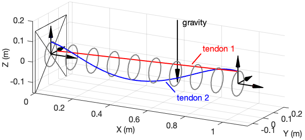
Figure 2: A continuum robot subject to gravity and tendon actuation.

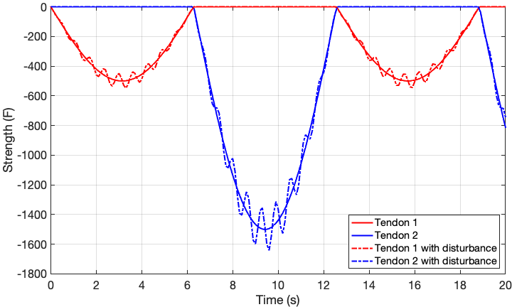
Figure 3: Strengths of the tendons.

The robot parameters are given in Table 1. The material damping is assumed to be 0 by default unless otherwise specified. The robot is subject to gravity and the actuation of two tendons; see Fig. 2. Tendon 1 is obliquely routed starting from $(x,y,z)=(0,0.06,0)$ to $(0,0,0.06)$. Tendon 2 is helically routed starting from $(x,y,z)=(0,0,0.06)$ and rotates with pitch $=0.16\mathrm{m/rad}$ in a clockwise direction. The robot is initially at equilibrium which is a bending configuration due to gravity. The two tendons are alternatively actuated to cause complicated 3D deformation of the robot. Their strengths are specified according to

$$T_{1}=-[500\sin(t/2)]_{+},$$

$$T_{2}=[1500\sin(t/2)]_{-},$$

respectively, where $f_{+}$ and $f_{-}$ represent the positive and negative parts of the function $f$; see Fig. 3. In SoRoSim, all the strains are set to be active and approximated by polynomials of order 0. The order of the Gauss quadrature for numerical spatial integration is set to be 10. The MATLAB ODE solver ‘ode45’ is chosen for numerical temporal integration.

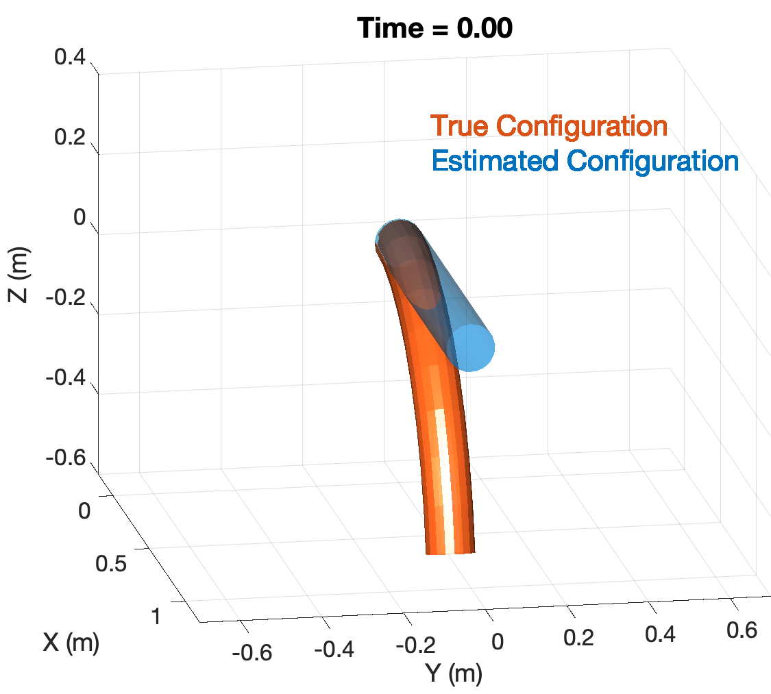
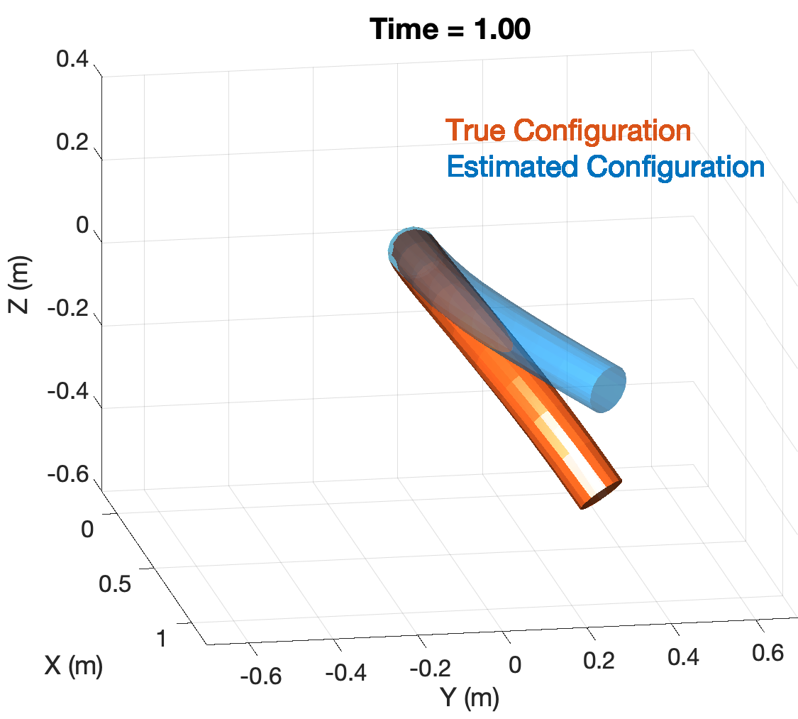
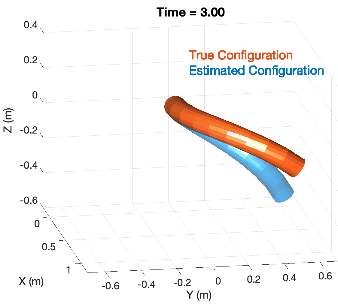
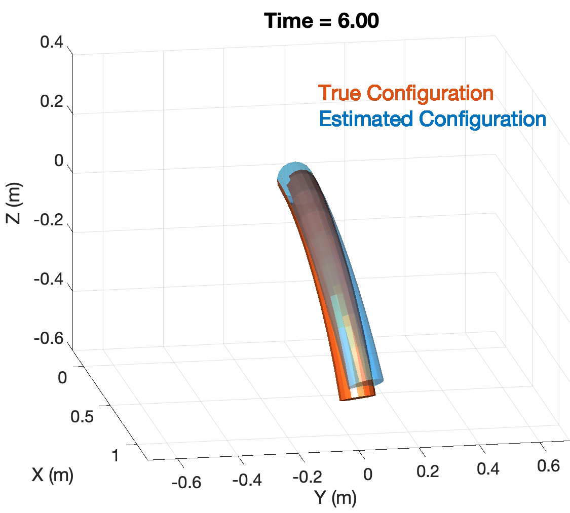
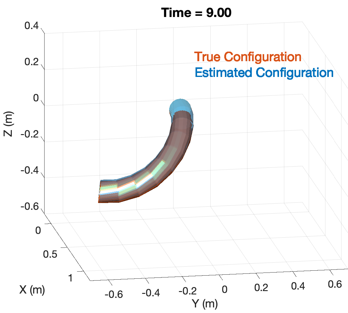
Figure 4: Comparison of the true configuration (red) and estimated configuration (blue). ($\Gamma=0.3I$.)

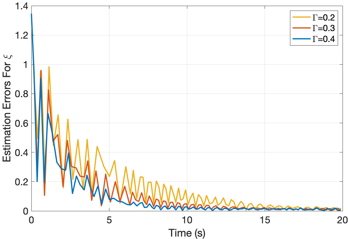
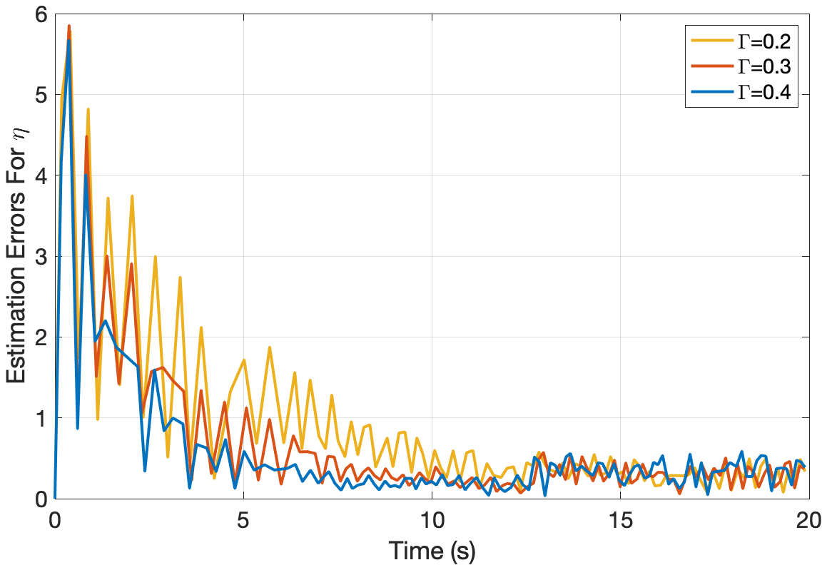
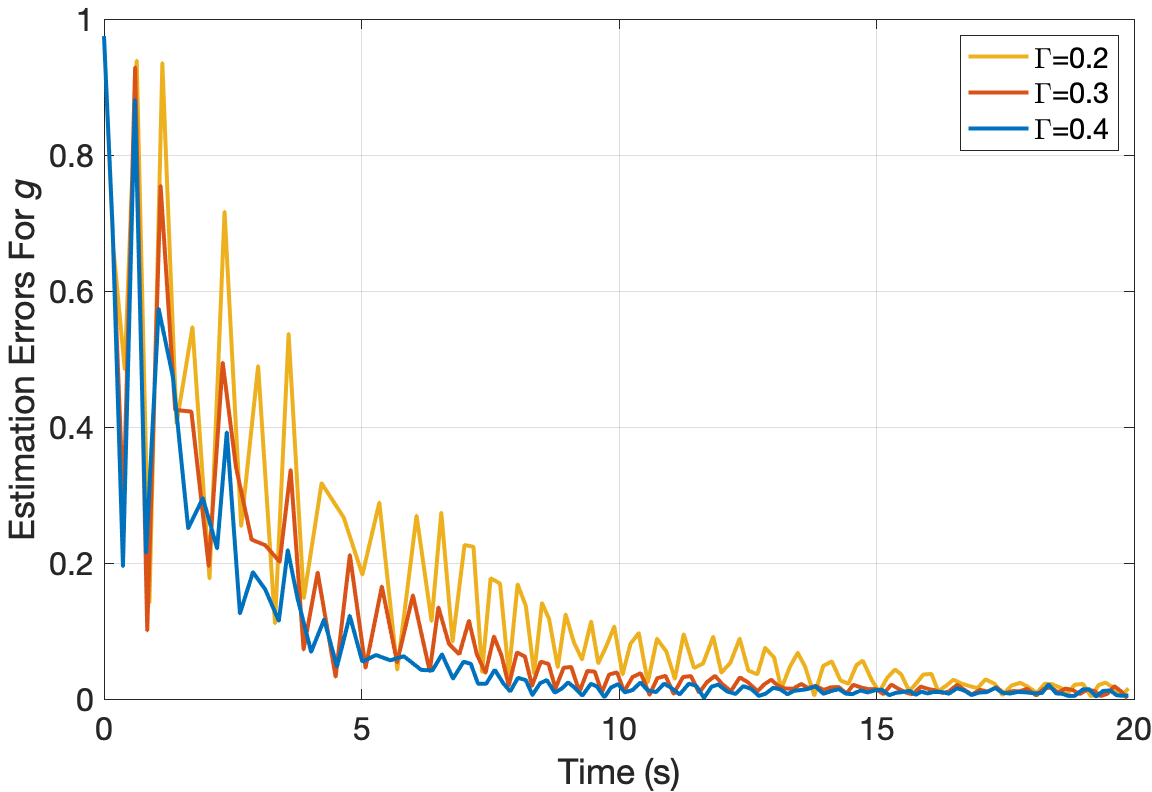
Figure 5: Estimation errors (from left to right) $\|\tilde{\xi}(\cdot,t)\|_{L^{\infty}}$, $\|\tilde{\eta}(\cdot,t)\|_{L^{\infty}}$, and $\|\tilde{g}(\cdot,t)\|_{L^{\infty}}$ for Experiment 1 – Impact of Observer Gains. No uncertainty is added.

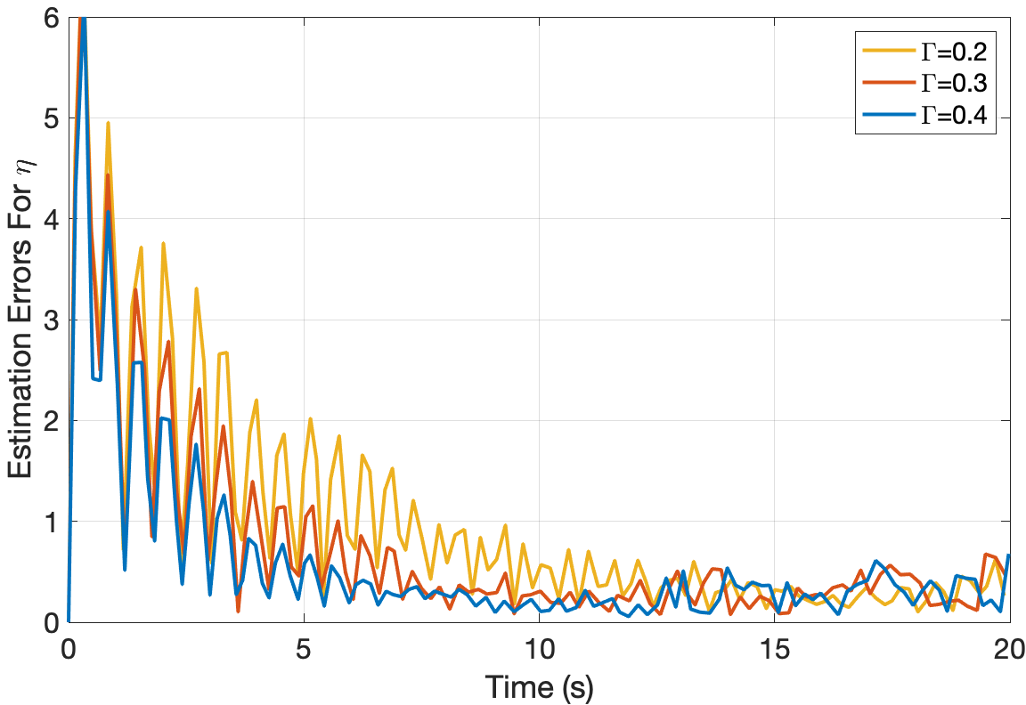
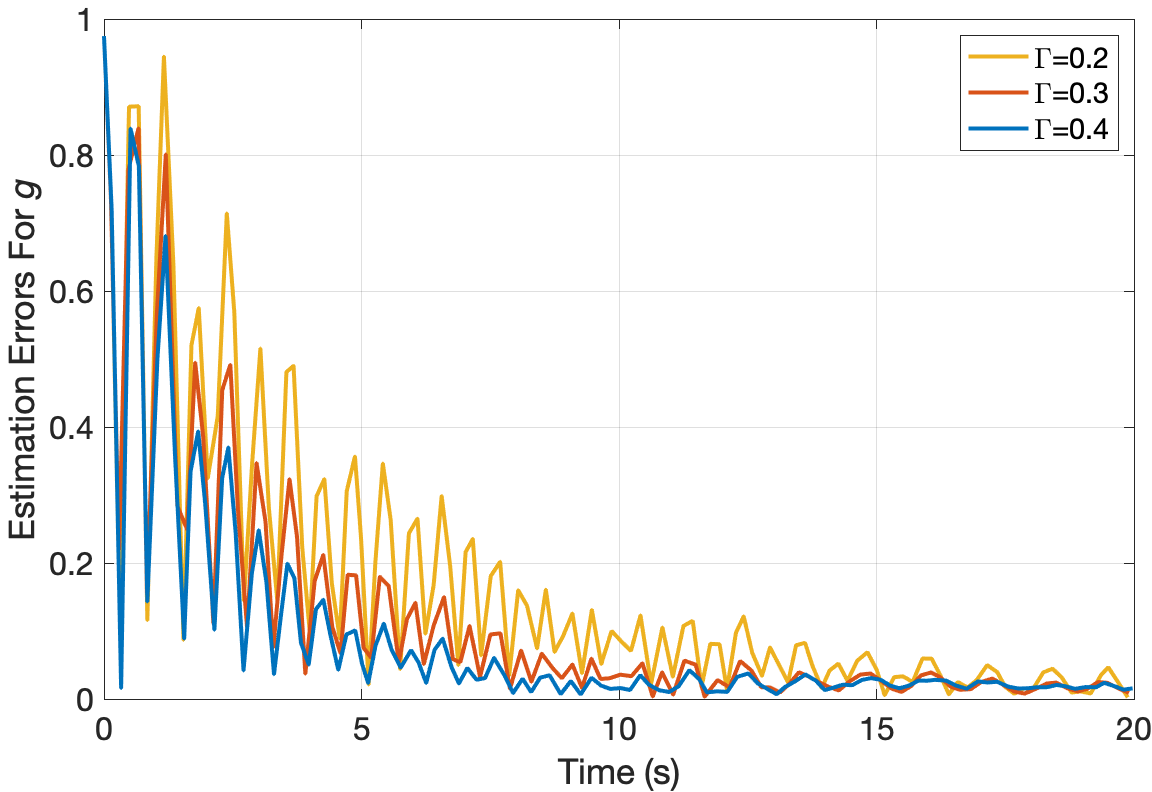
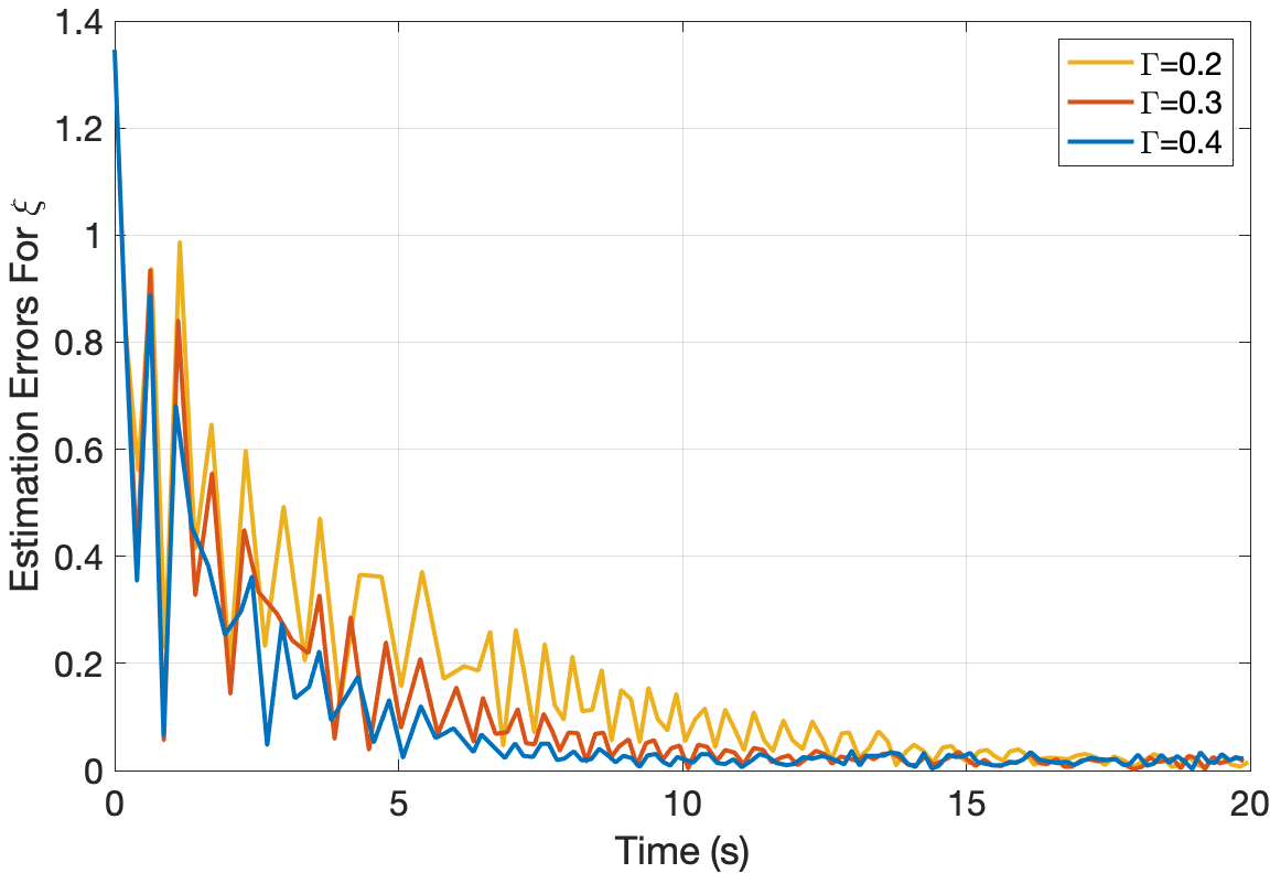
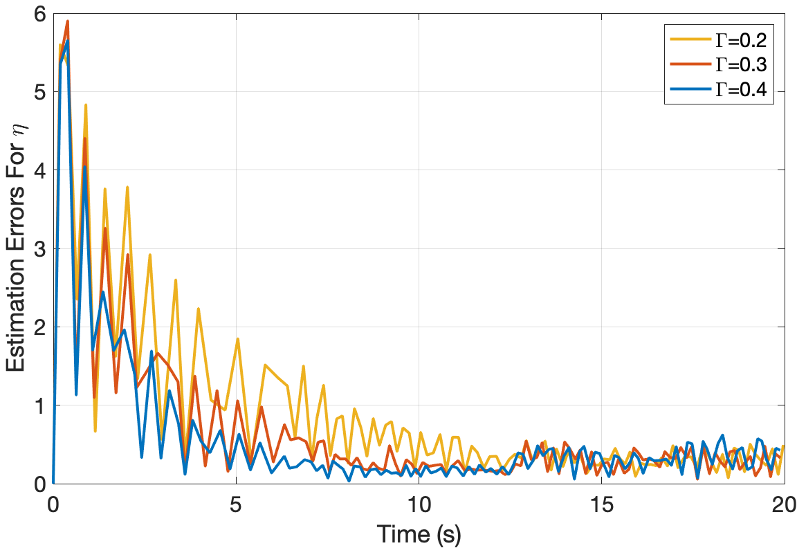
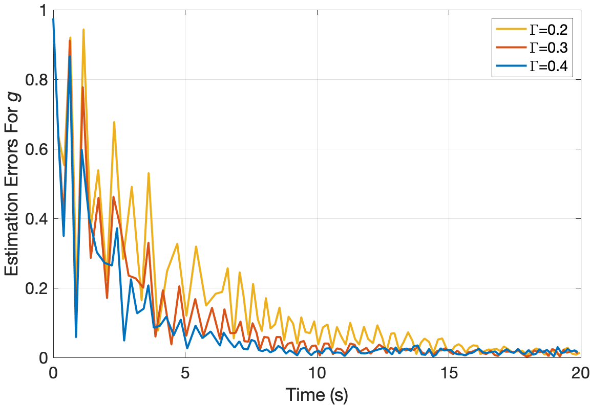
Figure 6: Estimation errors (from left to right) $\|\tilde{\xi}(\cdot,t)\|_{L^{\infty}}$, $\|\tilde{\eta}(\cdot,t)\|_{L^{\infty}}$, and $\|\tilde{g}(\cdot,t)\|_{L^{\infty}}$ for Experiment 2 – Impact of Tip Measurement Uncertainty. Temporally independent measurement noise and a temporally constant measurement bias are added to the top and the bottom, respectively.

The sampling rate of the tip velocity is set to be $200\mathrm{Hz}$. A boundary observer (13) is used to estimate the robot states. The initial estimate is set to be a straight configuration, which has a large initial estimation error. A series of independent experiments are performed to study the impact of different factors, such as observer gains, velocity measurement uncertainty, model parameter uncertainty, actuation input uncertainty, and material damping.

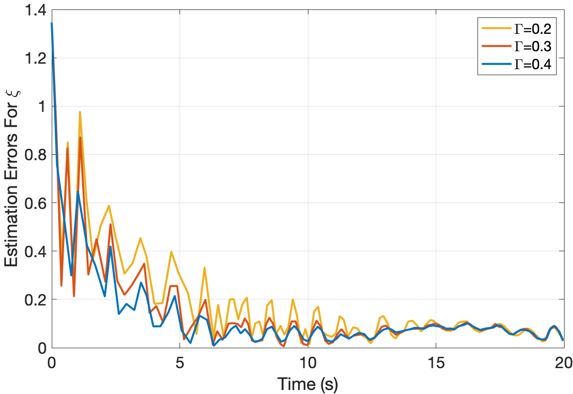
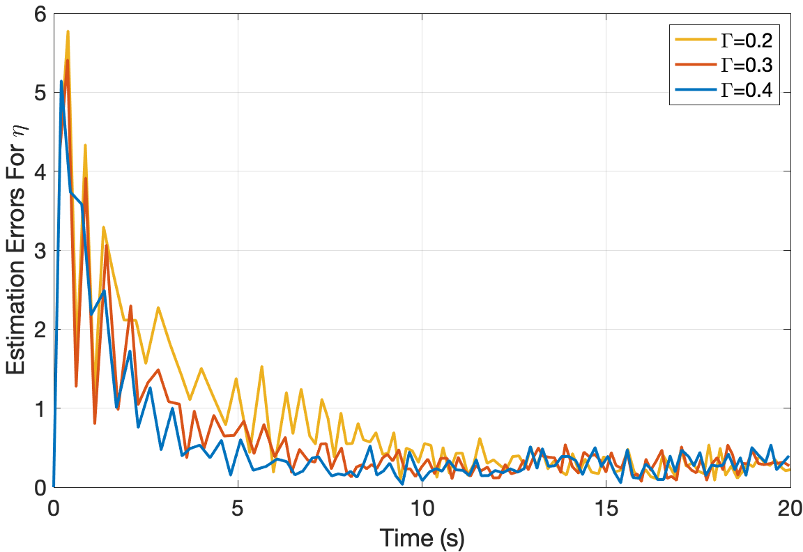
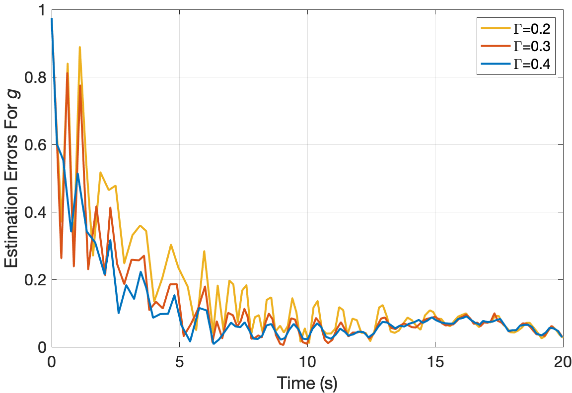
Figure 7: Estimation errors (from left to right) $\|\tilde{\xi}(\cdot,t)\|_{L^{\infty}}$, $\|\tilde{\eta}(\cdot,t)\|_{L^{\infty}}$, and $\|\tilde{g}(\cdot,t)\|_{L^{\infty}}$ for Experiment 3 – Impact of Model Uncertainty. A spatially varying but temporally constant bias is added to the stiffness and inertial matrices.

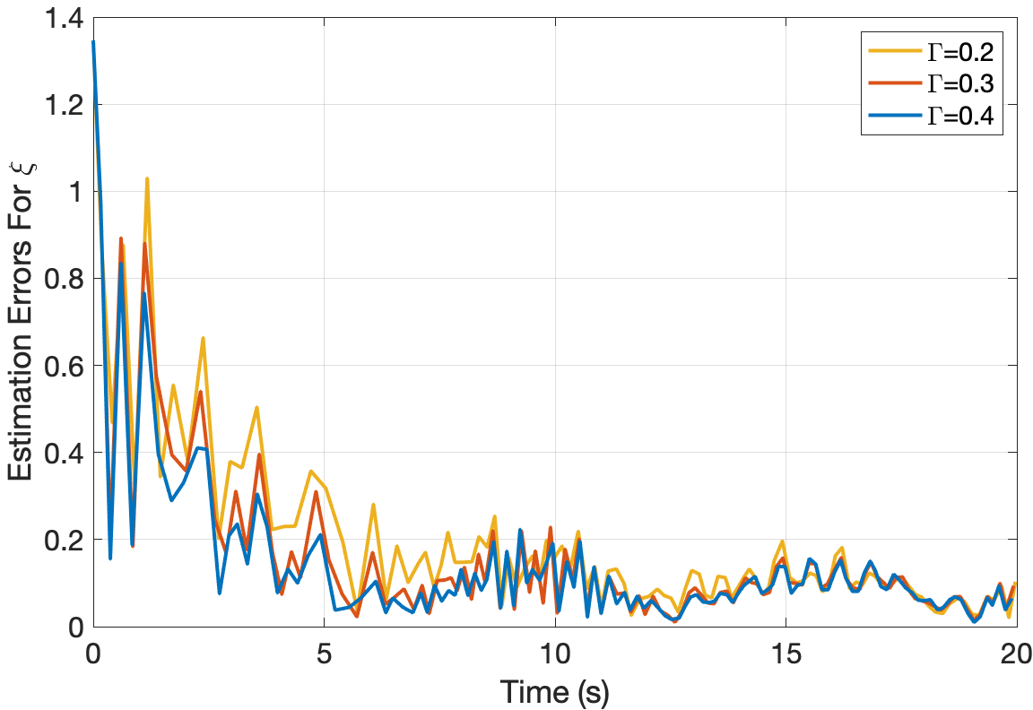
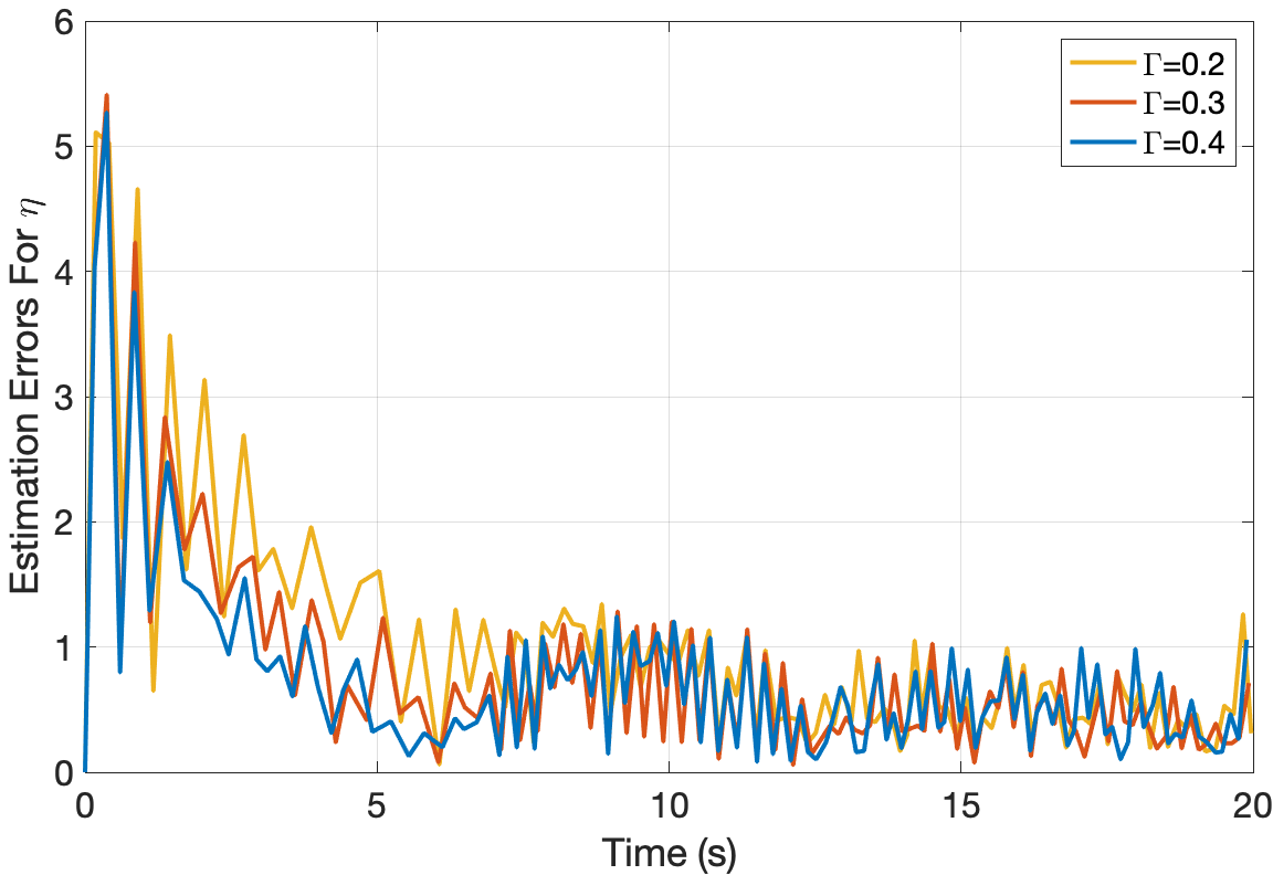
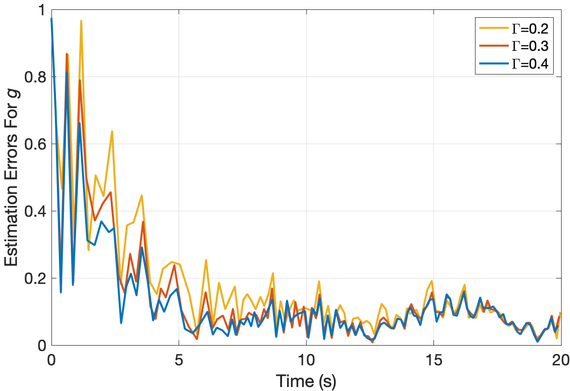
Figure 8: Estimation errors (from left to right) $\|\tilde{\xi}(\cdot,t)\|_{L^{\infty}}$, $\|\tilde{\eta}(\cdot,t)\|_{L^{\infty}}$, and $\|\tilde{g}(\cdot,t)\|_{L^{\infty}}$ for Experiment 4 – Impact of Input Uncertainty. Disturbance is added to the wrench generated by the tendons.

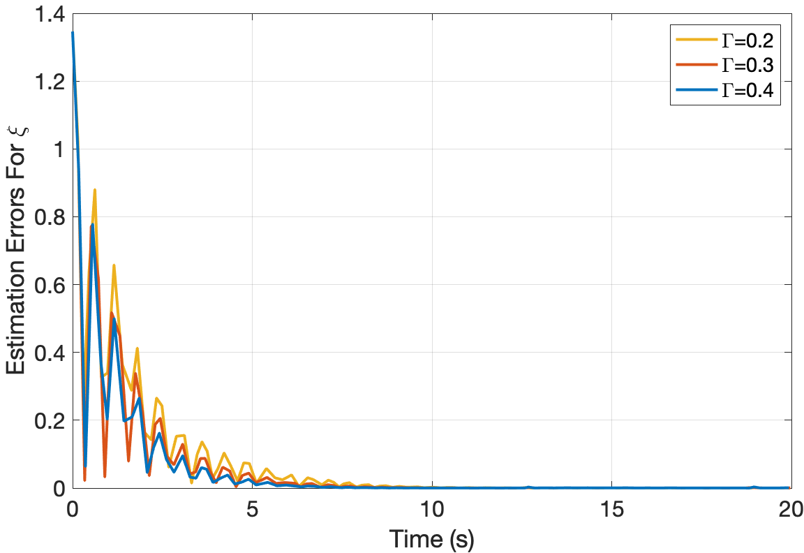
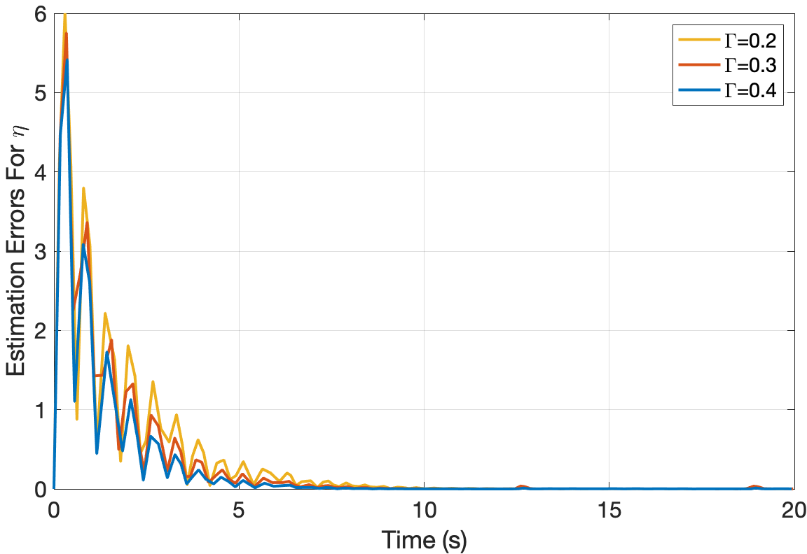
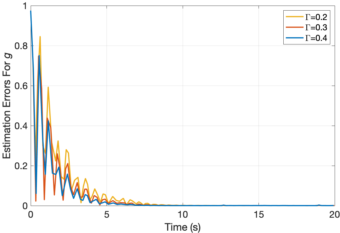
Figure 9: Estimation errors (from left to right) $\|\tilde{\xi}(\cdot,t)\|_{L^{\infty}}$, $\|\tilde{\eta}(\cdot,t)\|_{L^{\infty}}$, and $\|\tilde{g}(\cdot,t)\|_{L^{\infty}}$ for Experiment 5 – Impact of Material Damping. A constitutive law with damping is adopted for both the robot and the observer.

4.1 Experiment 1: Impact of Observer Gains

This experiment is to validate the theoretical results and hence no uncertainty is added. To study the impact of different observer gains, we set $\Gamma=0.2I,0.3I,0.4I$ where $I$ is the identity matrix.

Result. An illustration of the estimation process is given in Fig. 4. We observe that the estimated configuration gradually converges to the true configuration. The $L^{\infty}$ norms of estimation errors of all robot states are plotted in Fig. 5, which exhibit exponential convergence toward a small neighborhood of 0. This verifies the input-to-state stable property of the boundary observer. Moreover, larger observer gains always result in faster convergence. Although the theoretical results are only local, the large initial estimation errors suggest that the domain of attraction is large. The velocity estimates tend to have larger estimation errors than the strains and poses especially when the actuation switches to a different tendon. This is possibly because velocities are directly affected by the actuation and exhibit more sensitivity.

4.2 Experiment 2: Impact of Tip Measurement Uncertainty

The tip velocity measurements using, e.g., IMUs, usually contain disturbances. To study the robustness to measurement uncertainty of the tip velocities, we add two kinds of disturbance to the tip velocity measurements: noise and bias.

4.2.1 Experiment 2.1

At every $t$, temporally independent noise is drawn from a uniform distribution on the interval $[-20\%,20\%]$ of the average magnitude of the tip linear (angular) velocity and then added to each component of the tip linear (angular) velocity measurements.

4.2.2 Experiment 2.2

For all $t$, a temporally constant bias of $20\%$ of the average magnitude of the tip linear (angular) velocity is added to each component of the tip linear (angular) velocity measurements.

Result. The $L^{\infty}$ norms of estimation errors of all robot states are plotted in Fig. 6. Comparing it with Fig. 5, we observe that disturbances on tip velocity measurements only induce a very small amount of extra steady-state errors, which suggests that the boundary observer is very robust to tip measurement uncertainty.

4.3 Experiment 3: Impact of Model Uncertainty

In practice, the robot parameters may not be known exactly. To study the robustness to model uncertainty, spatially independent noise is drawn from a uniform distribution on the interval $[-20\%,20\%]$ once and then added to the stiffness and inertial matrices $K(s)$ and $J(s)$ as a temporally constant bias.

Result. The $L^{\infty}$ norms of estimation errors of all robot states are plotted in Fig. 7. Comparing it with Fig. 5, we observe that model uncertainty induces a small amount of extra steady-state errors, especially on the strains and poses. Nevertheless, the boundary observer exhibits reasonable robustness to model uncertainty.

4.4 Experiment 4: Impact of Input Uncertainty

In practice, it may be difficult to determine the exact amount of wrench generated by the actuators. To study the robustness to input uncertainty, we use the following perturbed input signals for the boundary observer; see Fig. 3 for illustration.

$$T_{1}=-[500\sin(t/2)(1+0.1\sin(10t))]_{+},$$

$$T_{2}=[1500\sin(t/2)(1+0.1\sin(10t))]_{-}.$$

Result. The $L^{\infty}$ norms of estimation errors of all robot states are plotted in Fig. 8. Comparing it with Fig. 5, we observe that uncertainty of input signals induces a moderate amount of extra steady-state errors on all robot states. This is not surprising because the central idea of the boundary observer is to dissipate energy from estimation errors while inaccurate input signals may induce extra energy into the estimation errors. Future work will study how to use additional sensing (like position measurements) to compensate for the input uncertainty.

4.5 Experiment 5: Impact of Material Damping

All the theoretical results in this work are based on assuming the linear constitutive law (9). This experiment is to validate that the presented boundary observer also works for the constitutive law with damping (11). We set the material damping to be $1.125\times 10^{4}\mathrm{Pa.s}$ and assume it is known. Correspondingly, we use (15) to compute $\hat{\phi}$ for the boundary observer.

Result. The $L^{\infty}$ norms of estimation errors of all robot states are plotted in Fig. 9. Comparing it with Fig. 5, we observe that the boundary observer exhibits better performance in terms of faster convergence rates and smaller steady-state errors. This is possibly because material damping results in slower motions, reduces oscillations, and helps dissipating energy.

Remark 4.3.

One can repeat Experiments 2-4 in the case when material damping is present and will find that similar robustness results also hold in this case.

4.6 Summary

In summary, although the theoretical stability is only local and requires a linear constitutive law, numerical studies suggest that the domain of attraction is large and the observer works well even with material damping. The observer turns out the be very robust to the tip measurement uncertainty, followed by the model uncertainty, and is most sensitive to the uncertainty of input signals.

5 Conclusion

In this work, we designed a boundary observer for continuum robotic arms based on Cosserat rod PDEs. This observer was able to estimate all infinite-dimensional continuum robot states from only tip velocity measurements, could be easily implemented in both the hardware and numerical aspects, and was proven to be locally input-to-state stable. Extensive numerical experiments were conducted which suggested that the domain of attraction was large and the observer was robust to uncertainties of tip velocity measurements and model parameters. These results suggested the promising role of PDE control theory for soft robots. Our future work includes theoretical studies on the robustness of the observer, using additional sensing data to improve the robustness, and testing it on physical platforms.

Appendix

5.1 Preliminaries for proving Theorem 1

The proof of Theorem 1 relies on some preliminary results from the work [34] which studies boundary stabilization of Cosserat rods. The main results are summarized here. Consider the following system with boundary control:

$$\left\{\begin{aligned} &\partial_{t}\xi=\partial_{s}\eta+ad_{\xi}\eta,\\ &J\partial_{t}\eta=\partial_{s}\phi-ad_{\xi}^{T}\phi+ad_{\eta}^{T}J\eta,\\ &\begin{aligned} &\phi(\ell,t)=-\Gamma\eta(\ell,t),\\ &\eta(0,t)=0,\\ &\phi(s,0)=\phi_{0}(s),\\ &\eta(s,0)=\eta_{0}(s),\end{aligned}\end{aligned}\right.$$ (21)

where $\Gamma\in\mathbb{R}^{6\times 6}$ is the feedback gain. The system (21) is related to (12) by (i) setting all the distributed inputs $\{\phi_{\text{loc}},\psi_{\text{loc}},\psi_{\text{glb}}\}$ (including gravity) to be 0, (ii) setting the boundary condition $\eta(0,t)$ to be 0, and (iii) setting the boundary condition $\phi(\ell,t)$ to be $-\Gamma\eta(\ell,t)$, which is the boundary controller in [34].

The total energy of (21), consisting of kinetic energy and (elastic) potential energy, is defined by

$$\mathcal{E}(t)=\int_{0}^{\ell}\eta^{T}J\eta+\phi^{T}K^{-1}\phi ds.$$

If $\Gamma=0$, it is well-known that the total energy is conserved, i.e., $\frac{d}{dt}\mathcal{E}(t)=0$. If $\Gamma>0$, one can show that

$$\frac{d}{dt}\mathcal{E}(t)=-2\eta^{T}(\ell,t)\Gamma\eta(\ell,t)\leq 0,$$

which implies the total energy is non-increasing, i.e., (21) is stable. However, it is not necessarily decreasing, or asymptotically stable. The authors of [34] then managed to prove that (21) is locally exponentially stable by finding a modulated quadratic Lyapunov functional. In particular, (21) can be rewritten as

$$\left\{\begin{aligned} &\partial_{t}y+A\partial_{s}y+By=F(y)\\ &\begin{aligned} &\phi(\ell,t)=-\Gamma\eta(\ell,t),\\ &\eta(0,t)=0,\\ &y(s,0)=y_{0}(s),\end{aligned}\end{aligned}\right.$$ (22)

where $A$, $B$, and $F$ are defined in the same way as in (19). The following theorems summarize the main results from [34].

Theorem 5.4 (Well-posedness).

For any $T>0$, there exists $\delta>0$ such that if $y_{0}$ satisfies $\|y_{0}\|_{H^{1}}\leq\delta$ and the compatibility conditions, then there exists a unique solution $y\in C^{0}([0,T),H^{1})$ to (22). Moreover, if $\|y(\cdot,t)\|_{H^{1}}\leq\delta$ for all $t\in[0,T)$, then $T=+\infty$.

Theorem 5.5 (Local exponential stability).

If $\Gamma$ is positive-definite, then (22) is locally exponentially stable in $H^{1}$. Moreover, a Lyapunov certificate is given by

$$\mathcal{V}(t)=\int_{0}^{\ell}y^{T}Py+\partial_{t}y^{T}P\partial_{t}yds$$

where $P\in C^{1}([0,\ell];\mathbb{R}^{12\times 12})$ satisfies

1. $P(s)$ is positive-definite for all $s\in[0,\ell]$,

2. $(PA)(s)$ is symmetric for all $s\in[0,\ell]$,

3. $Q:=-\frac{d}{ds}(PA)+PB+B^{T}P$ is positive-definite for all $s\in[0,\ell]$,

4. $(y^{T}PAy)(\ell,t)-(y^{T}PAy)(0,t)\geq 0$ for all $t$.

5.2 Proof of Theorem 1

Proof 5.6.

By suitably renaming the variables, (19) can be seen as a perturbation of (22) with the injection of the nonlinear terms $G$ and $H$. The main idea of our proof is to extend the original proof (in [34]) of Theorem 5.5 to accommodate the terms $G$ and $H$ and establish local input-to-state stability. Throughout the proof, all norms are defined only on the $s$ variable and we also omit the dependence on $t$ for brevity.

Let $P$ satisfy all the properties in Theorem 5.5. Define Lyapunov functionals

$$\mathcal{V}_{0}(t) =\int_{0}^{\ell}\tilde{y}^{T}P\tilde{y}ds,$$

$$\mathcal{V}_{1}(t) =\int_{0}^{\ell}\partial_{t}\tilde{y}^{T}P\partial_{t}\tilde{y}ds.$$

Let $\mathcal{V}=\mathcal{V}_{0}+\mathcal{V}_{1}$. We will show that $\mathcal{V}$ is equivalent to $\|\tilde{y}\|_{H^{1}}$ later in (28). Differentiating $\mathcal{V}_{0}$, substituting (19), and then using integration by parts and the properties of $P$, we have

$$\dot{\mathcal{V}}_{0} =\int_{0}^{\ell}2\tilde{y}^{T}P\big{[}-A\partial_{s}\tilde{y}-B\tilde{y}$$

$$\quad+F(\tilde{y})+G(y,\tilde{y})+H(d,\tilde{R},\tilde{y})\big{]}ds$$

$$=-\tilde{y}^{T}PA\tilde{y}\mid_{0}^{\ell}+\int_{0}^{\ell}\tilde{y}^{T}\partial_{s}(PA)\tilde{y}+\partial_{s}\tilde{y}^{T}PA\tilde{y}$$

$$\quad-\tilde{y}^{T}PA\partial_{s}\tilde{y}-\tilde{y}^{T}PB\tilde{y}-\tilde{y}^{T}B^{T}P\tilde{y}$$

$$\quad+\tilde{y}^{T}P\big{[}F(\tilde{y})+G(y,\tilde{y})+H(d,\tilde{R},\tilde{y})\big{]}ds$$

$$\leq\int_{0}^{\ell}-\tilde{y}^{T}Q\tilde{y}+\tilde{y}^{T}P\big{[}F(\tilde{y})+G(y,\tilde{y})+H(d,\tilde{R},\tilde{y})\big{]}ds,$$

where the term $\tilde{y}^{T}PA\tilde{y}\mid_{0}^{\ell}\geq 0$ by the forth property of $P$ and $Q:=-\partial_{s}(PA)+PB+B^{T}P$ is positive-definite by the third property of $P$ in Theorem 5.5. By a similar derivation,

$$\dot{\mathcal{V}}_{1} \leq\int_{0}^{\ell}-\partial_{t}\tilde{y}^{T}Q\partial_{t}\tilde{y}$$

$$\quad+\partial_{t}\tilde{y}^{T}P\partial_{t}\big{[}F(\tilde{y})+G(y,\tilde{y})+H(d,\tilde{R},\tilde{y})\big{]}ds.$$

Thus, there exist a constant $C_{0}>0$ such that

$$\begin{split}\dot{\mathcal{V}}&\leq-C_{0}\mathcal{V}+\sum_{i=0}^{1}\int_{0}^{\ell}\partial_{t}^{i}\tilde{y}^{T}P\partial_{t}^{i}\big{[}F(\tilde{y})\\ &\quad+G(y,\tilde{y})+H(d,\tilde{R},\tilde{y})\big{]}ds.\end{split}$$ (23)

Now we need to derive some estimates for the nonlinear terms $F$, $G$, and $H$. From now on, we assume there exist constants $\delta$, $\gamma_{1}$, $\gamma_{2}>0$ such that $\|\tilde{y}\|_{H^{1}}<\delta$, $\|y\|_{H^{1}}<\gamma_{1}$, and $\|d\|_{H}<\gamma_{2}$ for all $t$. By the Sobolev inequality [35], we correspondingly have $\|\tilde{y}\|_{L^{\infty}}<c_{0}\delta$, $\|y\|_{L^{\infty}}<c_{1}\gamma_{1}$, and $\|d\|_{L^{\infty}}<c_{2}\gamma_{2}$ for some constants $c_{0},c_{1},c_{2}>0$.

By definition, $F(y)$ is a matrix-valued quadratic function consisting of only square terms. By Hölder’s inequality [35], there exist constants $c_{3},c_{4}>0$ such that

$$\int_{0}^{\ell}\tilde{y}^{T}PF(\tilde{y})ds\leq c_{3}\|\tilde{y}\|_{L^{\infty}}\|\tilde{y}\|_{L^{2}}^{2}\leq c_{0}c_{3}\delta\|\tilde{y}\|_{L^{2}}^{2},$$

$$\int_{0}^{\ell}\partial_{t}\tilde{y}^{T}P\partial_{t}F(\tilde{y})ds\leq c_{4}\|\tilde{y}\|_{L^{\infty}}\|\partial_{t}\tilde{y}\|_{L^{2}}^{2}\leq c_{0}c_{4}\delta\|\partial_{t}\tilde{y}\|_{L^{2}}^{2}.$$

The above estimates imply that there exists a constant $C_{1}>0$ such that

$$\sum_{i=0}^{1}\int_{0}^{\ell}\partial_{t}^{i}\tilde{y}^{T}P\partial_{t}^{i}F(\tilde{y})ds\leq C_{1}\delta\mathcal{V}.$$ (24)

By definition, $G(y,\tilde{y})$ is a matrix-valued bilinear function. By Hölder’s inequality, there exist constants $c_{5},c_{6},c_{7}>0$ such that

$$\int_{0}^{\ell} \tilde{y}^{T}PG(y,\tilde{y})ds$$

$$\leq c_{5}\|\tilde{y}\|_{L^{\infty}}\|\tilde{y}\|_{L^{2}}\|y\|_{L^{2}}\leq c_{1}c_{5}\delta\|\tilde{y}\|_{L^{2}}\|y\|_{L^{2}},$$

$$\int_{0}^{\ell} \partial_{t}\tilde{y}^{T}P\partial_{t}G(y,\tilde{y})ds$$

$$\leq c_{6}\|\tilde{y}\|_{L^{\infty}}\|\partial_{t}\tilde{y}\|_{L^{2}}\|\partial_{t}y\|_{L^{2}}+c_{7}\|y\|_{L^{\infty}}\|\partial_{t}\tilde{y}\|_{L^{2}}^{2}$$

$$\leq c_{0}c_{6}\delta\|\partial_{t}\tilde{y}\|_{L^{2}}\|\partial_{t}y\|_{L^{2}}+c_{1}c_{7}\gamma_{1}\|\partial_{t}\tilde{y}\|_{L^{2}}^{2}.$$

The above estimates, together with the fact that $\sum_{i=0}^{1}\|\partial_{t}^{i}y\|_{L^{2}}$ is locally equivalent to $\|y\|_{H^{1}}$ ([34], p.p. 23), imply that there exist constants $C_{2},C_{3}>0$ such that

$$\begin{split}\sum_{i=0}^{1}\int_{0}^{\ell}&\partial_{t}^{i}\tilde{y}^{T}P\partial_{t}^{i}G(y,\tilde{y})ds\\ &\leq C_{2}\delta\sqrt{\mathcal{V}}\|y\|_{H^{1}}+C_{3}\gamma_{1}\mathcal{V}.\end{split}$$ (25)

According to the definition of $\bar{H}$ in (18), we can denote $H(d,\tilde{R},\tilde{y})=H_{1}(d,\tilde{y})+H_{2}(d,\tilde{R})$ where $H_{1}$ is the portion involving $ad_{K^{-1}\tilde{\phi}}\phi_{\text{loc}}$ and $H_{2}$ is the portion involving $\tilde{R}^{T}\psi_{\text{glb}}$. By definition, $H_{1}(d,\tilde{y})$ and $H_{2}(d,\tilde{R})$ are both matrix-valued bilinear functions. $H_{1}(d,\tilde{y})$ can be easily tackled in a similar way as $G(y,\tilde{y})$. In particular, we can deduce that there exist constants $C_{4},C_{5}>0$ such that

$$\begin{split}\sum_{i=0}^{1}\int_{0}^{\ell}&\partial_{t}^{i}\tilde{y}^{T}P\partial_{t}^{i}H_{1}(d,\tilde{y})ds\\ &\leq C_{4}\delta\sqrt{\mathcal{V}}\|d\|_{H}+C_{5}\gamma_{2}\mathcal{V}.\end{split}$$ (26)

Now we focus on $H_{2}(d,\tilde{R})$. According to (2), $\partial_{s}R=Ru^{\wedge}$ where $u$ is the angular component of the strain $\xi$ and therefore part of $y$. Since $\tilde{R}(0,t)=0$ for all $t$, by the fundamental theorem of calculus, there exists a constant $c_{8}>0$ depending on $\ell$ such that

$$\|\tilde{R}\|_{L^{\infty}} \leq c_{8}\|\partial_{s}\tilde{R}\|_{L^{\infty}}$$

$$=c_{8}\|\hat{R}\hat{u}^{\wedge}-\hat{R}u^{\wedge}+\hat{R}u^{\wedge}-Ru^{\wedge}\|_{L^{\infty}}$$

$$\leq c_{8}\|\hat{R}\tilde{u}^{\wedge}\|_{L^{\infty}}+c_{8}\|\tilde{R}\|_{L^{\infty}}\|u\|_{L^{\infty}}$$

$$\leq c_{9}\|\tilde{u}\|_{L^{\infty}}+c_{1}c_{8}\gamma_{1}\|\tilde{R}\|_{L^{\infty}},$$

for some constant $c_{9}>0$, where we have used the fact that a rotation matrix $\hat{R}$ has a bounded matrix norm. Thus, by choosing $\gamma_{1}$ to be sufficiently small, we have

$$\|\tilde{R}\|_{L^{\infty}}\leq\frac{c_{9}}{1-c_{1}c_{8}\gamma_{1}}\|\tilde{y}\|_{L^{\infty}}=:c_{10}\|\tilde{y}\|_{L^{\infty}},$$

for some constant $c_{10}>0$. By a similar argument as $\partial_{s}\tilde{R}$ and the fact that $\partial_{t}R=Rw^{\wedge}$ where $w$ is the angular component of the velocity $\eta$ and therefore part of $y$, there exists a constant $c_{11}>0$ such that

$$\|\partial_{t}\tilde{R}\|_{L^{\infty}} \leq c_{11}\|\tilde{w}\|_{L^{\infty}}+c_{1}\gamma_{1}\|\tilde{R}\|_{L^{\infty}}$$

$$\leq c_{11}\|\tilde{y}\|_{L^{\infty}}+c_{1}c_{10}\gamma_{1}\|\tilde{y}\|_{L^{\infty}}=:c_{12}\|\tilde{y}\|_{L^{\infty}},$$

for some constant $c_{12}>0$. Now, by Hölder’s inequality, there exist constants $c_{13},c_{14}>0$ such that

$$\int_{0}^{\ell} \tilde{y}^{T}PH_{2}(d,\tilde{R})ds$$

$$\leq c_{13}\|\tilde{y}\|_{L^{2}}\|\tilde{R}\|_{L^{\infty}}\|\psi_{\text{glb}}\|_{L^{2}}\leq c_{0}c_{10}c_{13}\delta\|\tilde{y}\|_{L^{2}}\|\psi_{\text{glb}}\|_{L^{2}},$$

$$\int_{0}^{\ell} \partial_{t}\tilde{y}^{T}P\partial_{t}H_{2}(d,\tilde{R})ds$$

$$\leq\int_{0}^{\ell}\partial_{t}\tilde{y}^{T}P\big{[}(\partial_{t}\tilde{R}^{T})\psi_{\text{glb}}+\tilde{R}^{T}\partial_{t}\psi_{\text{glb}}\big{]}ds$$

$$\leq c_{14}\|\partial_{t}\tilde{y}\|_{L^{2}}(\|\partial_{t}\tilde{R}\|_{L^{\infty}}\|\psi_{\text{glb}}\|_{L^{2}}+\|\tilde{R}\|_{L^{\infty}}\|\partial_{t}\psi_{\text{glb}}\|_{L^{2}})$$

$$\leq c_{0}c_{14}\delta\|\partial_{t}\tilde{y}\|_{L^{2}}(c_{12}\|\psi_{\text{glb}}\|_{L^{2}}+c_{10}\|\partial_{t}\psi_{\text{glb}}\|_{L^{2}}).$$

The above estimates imply that there exists a constant $C_{6}>0$ such that

$$\begin{split}\sum_{i=0}^{1}\int_{0}^{\ell}\partial_{t}^{i}\tilde{y}^{T}P\partial_{t}^{i}H_{2}(d,\tilde{R})ds\leq C_{6}\delta\sqrt{\mathcal{V}}\|d\|_{H}.\end{split}$$ (27)

We also need to show that $\mathcal{V}$ is equivalent to $\|\tilde{y}\|_{H^{1}}$. Since the governing system of (19) is of first order in space and time, it yields a relationship between $\partial_{t}\tilde{y}$ and $\partial_{s}\tilde{y}$. In particular, using

$$\partial_{t}\tilde{y} =-A\partial_{s}\tilde{y}-B\tilde{y}+F(\tilde{y})+G(y,\tilde{y})+H(d,\tilde{R},\tilde{y}),$$

$$\partial_{s}\tilde{y} =A^{-1}\big{(}-\partial_{t}\tilde{y}-B\tilde{y}+F(\tilde{y})+G(y,\tilde{y})+H(d,\tilde{R},\tilde{y})\big{)},$$

we can deduce that there exists a constant $\epsilon$, depending on $A$, $B$, $\delta$, $\gamma_{1}$, $\gamma_{2}$, such that

$$\frac{1}{\epsilon}\sum_{i=0}^{1}|\partial_{s}^{i}\tilde{y}|^{2}\leq\sum_{i=0}^{1}|\partial_{t}^{i}\tilde{y}|^{2}\leq\epsilon\sum_{i=0}^{1}|\partial_{s}^{i}\tilde{y}|^{2},$$ (28)

which implies that $\mathcal{V}$ and $\|\tilde{y}\|_{H^{1}}$ are equivalent. Thus, any stability results for $\mathcal{V}$ implies similar results for $\|\tilde{y}\|_{H^{1}}$.

Now, using (23)-(27), we have

$$\dot{\mathcal{V}} \leq-(C_{0}-C_{1}\delta-C_{3}\gamma_{1}-C_{5}\gamma_{2})\mathcal{V}$$

$$\quad+\delta\sqrt{\mathcal{V}}\big{(}C_{2}\|y\|_{H^{1}}+(C_{4}+C_{6})\|d\|_{H}\big{)}$$

$$=:-C\mathcal{V}+\sqrt{\mathcal{V}}\mathcal{X},$$

where $C=C_{0}-C_{1}\delta-C_{3}\gamma_{1}-C_{5}\gamma_{2}$ and $\mathcal{X}=\delta\big{(}C_{2}\|y\|_{H^{1}}+(C_{4}+C_{6})\|d\|_{H}\big{)}$. We can let $\delta,\gamma_{1},\gamma_{2}$ be sufficiently small such that $C>0$. Let $\theta\in(0,1)$ be a constant. Then whenever $\sqrt{\mathcal{V}}\geq\frac{1}{C\theta}\mathcal{X}$, we have

$$\dot{\mathcal{V}} \leq-C(1-\theta)\mathcal{V}-C\theta\mathcal{V}+\sqrt{\mathcal{V}}\mathcal{X}$$

$$\leq-C(1-\theta)\mathcal{V}.$$

By invoking the Lyapunov function theorem for input-to-state stability [32, 36] and the equivalence of $\mathcal{V}$ and $\|\tilde{y}\|_{H^{1}}$, we obtain the desired results.

References

- [1] C. Laschi, B. Mazzolai, and M. Cianchetti, “Soft robotics: Technologies and systems pushing the boundaries of robot abilities,” Science robotics, vol. 1, no. 1, p. eaah3690, 2016.
- [2] M. L. Castaño and X. Tan, “Model predictive control-based path-following for tail-actuated robotic fish,” Journal of Dynamic Systems, Measurement, and Control, vol. 141, no. 7, 2019.
- [3] R. Sepulchre, “Control challenges for soft robotics [about this issue],” IEEE Control Systems Magazine, vol. 43, no. 3, pp. 5–7, 2023.
- [4] C. Della Santina, C. Duriez, and D. Rus, “Model-based control of soft robots: A survey of the state of the art and open challenges,” IEEE Control Systems Magazine, vol. 43, no. 3, pp. 30–65, 2023.
- [5] S. Song, Z. Li, H. Yu, and H. Ren, “Electromagnetic positioning for tip tracking and shape sensing of flexible robots,” IEEE Sensors Journal, vol. 15, no. 8, pp. 4565–4575, 2015.
- [6] H. Bezawada, C. Woods, and V. Vikas, “Shape estimation of soft manipulators using piecewise continuous pythagorean-hodograph curves,” in 2022 American Control Conference (ACC). IEEE, 2022, pp. 2905–2910.
- [7] P. L. Anderson, A. W. Mahoney, and R. J. Webster, “Continuum reconfigurable parallel robots for surgery: Shape sensing and state estimation with uncertainty,” IEEE robotics and automation letters, vol. 2, no. 3, pp. 1617–1624, 2017.
- [8] S. Lilge, T. D. Barfoot, and J. Burgner-Kahrs, “Continuum robot state estimation using gaussian process regression on se (3),” The International Journal of Robotics Research, vol. 41, no. 13-14, pp. 1099–1120, 2022.
- [9] C. Armanini, F. Boyer, A. T. Mathew, C. Duriez, and F. Renda, “Soft robots modeling: A structured overview,” IEEE Transactions on Robotics, 2023.
- [10] G. S. Chirikjian, “Hyper-redundant manipulator dynamics: A continuum approximation,” Advanced Robotics, vol. 9, no. 3, pp. 217–243, 1994.
- [11] C. Della Santina, R. K. Katzschmann, A. Bicchi, and D. Rus, “Model-based dynamic feedback control of a planar soft robot: trajectory tracking and interaction with the environment,” The International Journal of Robotics Research, vol. 39, no. 4, pp. 490–513, 2020.
- [12] J. C. Simo and L. Vu-Quoc, “On the dynamics in space of rods undergoing large motions—a geometrically exact approach,” Computer methods in applied mechanics and engineering, vol. 66, no. 2, pp. 125–161, 1988.
- [13] A. Macchelli, C. Melchiorri, and S. Stramigioli, “Port-based modeling of a flexible link,” IEEE transactions on robotics, vol. 23, no. 4, pp. 650–660, 2007.
- [14] D. C. Rucker and R. J. Webster III, “Statics and dynamics of continuum robots with general tendon routing and external loading,” IEEE Transactions on Robotics, vol. 27, no. 6, pp. 1033–1044, 2011.
- [15] F. Renda, M. Giorelli, M. Calisti, M. Cianchetti, and C. Laschi, “Dynamic model of a multibending soft robot arm driven by cables,” IEEE Transactions on Robotics, vol. 30, no. 5, pp. 1109–1122, 2014.
- [16] S. Grazioso, G. Di Gironimo, and B. Siciliano, “A geometrically exact model for soft continuum robots: The finite element deformation space formulation,” Soft robotics, vol. 6, no. 6, pp. 790–811, 2019.
- [17] F. Boyer, V. Lebastard, F. Candelier, and F. Renda, “Dynamics of continuum and soft robots: A strain parameterization based approach,” IEEE Transactions on Robotics, vol. 37, no. 3, pp. 847–863, 2020.
- [18] A. Mattioni, Y. Wu, H. Ramirez, Y. Le Gorrec, and A. Macchelli, “Modelling and control of an ipmc actuated flexible structure: A lumped port hamiltonian approach,” Control Engineering Practice, vol. 101, p. 104498, 2020.
- [19] J. Y. Loo, C. P. Tan, and S. G. Nurzaman, “H-infinity based extended kalman filter for state estimation in highly non-linear soft robotic system,” in 2019 American Control Conference (ACC). IEEE, 2019, pp. 5154–5160.
- [20] K. Stewart, Z. Qiao, and W. Zhang, “State estimation and control with a robust extended kalman filter for a fabric soft robot,” IFAC-PapersOnLine, vol. 55, no. 37, pp. 25–30, 2022.
- [21] T. Zheng and H. Lin, “Pde-based dynamic control and estimation of soft robotic arms,” in 2022 IEEE 61st Conference on Decision and Control (CDC). IEEE, 2022, pp. 2702–2707.
- [22] R. M. Murray, Z. Li, and S. S. Sastry, A mathematical introduction to robotic manipulation. CRC press, 2017.
- [23] R. Vazquez, M. Krstic, and J.-M. Coron, “Backstepping boundary stabilization and state estimation of a linear hyperbolic system,” in 2011 50th IEEE conference on decision and control and european control conference. IEEE, 2011, pp. 4937–4942.
- [24] F. Castillo, E. Witrant, C. Prieur, and L. Dugard, “Boundary observers for linear and quasi-linear hyperbolic systems with application to flow control,” Automatica, vol. 49, no. 11, pp. 3180–3188, 2013.
- [25] A. T. Mathew, I. M. B. Hmida, C. Armanini, F. Boyer, and F. Renda, “Sorosim: A matlab toolbox for hybrid rigid-soft robots based on the geometric variable-strain approach,” IEEE Robotics & Automation Magazine, 2022.
- [26] T. Zheng, Q. Han, and H. Lin, “Task space tracking of soft manipulators: Inner-outer loop control based on cosserat-rod models,” in 2023 American Control Conference (ACC), 2023.
- [27] F. Renda, C. Armanini, V. Lebastard, F. Candelier, and F. Boyer, “A geometric variable-strain approach for static modeling of soft manipulators with tendon and fluidic actuation,” IEEE Robotics and Automation Letters, vol. 5, no. 3, pp. 4006–4013, 2020.
- [28] M. S. Xavier, A. J. Fleming, and Y. K. Yong, “Finite element modeling of soft fluidic actuators: Overview and recent developments,” Advanced Intelligent Systems, vol. 3, no. 2, p. 2000187, 2021.
- [29] R. Mahony, T. Hamel, and J.-M. Pflimlin, “Nonlinear complementary filters on the special orthogonal group,” IEEE Transactions on automatic control, vol. 53, no. 5, pp. 1203–1218, 2008.
- [30] G. Bastin and J.-M. Coron, Stability and boundary stabilization of 1-d hyperbolic systems. Springer, 2016, vol. 88.
- [31] H. K. Khalil and J. W. Grizzle, Nonlinear systems. Prentice hall Upper Saddle River, NJ, 2002, vol. 3.
- [32] S. Dashkovskiy and A. Mironchenko, “Input-to-state stability of infinite-dimensional control systems,” Mathematics of Control, Signals, and Systems, vol. 25, no. 1, pp. 1–35, 2013.
- [33] T.-T. Li and Y. Jin, “Semi-global c1 solution to the mixed initial-boundary value problem for quasilinear hyperbolic systems,” Chinese Annals of Mathematics, vol. 22, no. 03, pp. 325–336, 2001.
- [34] C. Rodriguez, “Networks of geometrically exact beams: Well-posedness and stabilization,” Mathematical Control and Related Fields, vol. 12, no. 1, pp. 49–80, 2022.
- [35] L. C. Evans, Partial differential equations, ser. Graduate Studies in Mathematics. Providence, RI: American Mathematical Society, 1998.
- [36] T. Zheng, Q. Han, and H. Lin, “Transporting robotic swarms via mean-field feedback control,” IEEE Transactions on Automatic Control, vol. 67, no. 8, pp. 4170–4177, 2021.