The University of Michigan, Ann Arbor, MI 48109-1040, USAbbinstitutetext: Department of Physics, Pennsylvania State University, University Park, PA 16802, USAccinstitutetext: Kavli Institute for Theoretical Physics, University of California, Santa Barbara, CA 93106, USA
The Sub-Leading Scattering Waveform from Amplitudes
Abstract
We compute the next-to-leading order term in the scattering waveform of uncharged black holes in classical general relativity and of half-BPS black holes in supergravity. We propose criteria, generalizing explicit calculations at next-to-leading order, for determining the terms in amplitudes that contribute to local observables. For general relativity, we construct the relevant classical integrand through generalized unitarity in two distinct ways, (1) in a heavy-particle effective theory and (2) in general relativity minimally-coupled to scalar fields. With a suitable prescription for the matter propagator in the former, we find agreement between the two methods, thus demonstrating the absence of interference of quantum and classically-singular contributions. The classical integrand for massive scalar fields is constructed through dimensional reduction of the known five-point one-loop integrand. Our calculation exhibits novel features compared to conservative calculations and inclusive observables, such as the appearance of master integrals with intersecting matter lines and the appearance of a classical infrared divergence whose absence from classical observables requires a suitable definition of the retarded time.
1 Introduction
Much like accelerated charges in Maxwell’s theory emit electromagnetic radiation, accelerated masses in gravitational theories emit gravitational radiation. Increasingly more precise waveform models, yielding the asymptotic space-time metric, play a critical role in the detection and analysis of gravitational wave signals from compact binaries LIGOScientific:2021djp . Current waveform computations for binaries in bound orbits use effective-one-body methods Buonanno:1998gg ; Damour:2000we ; Buonanno:2000ef ; Damour:2001tu ; Damour:2014sva and numerical-relativity approaches Pretorius:2005gq ; Pretorius:2007nq , in addition to direct solutions of Einstein’s equations sourced by the motion of the bodies in the post-Newtonian approximation Blanchet:2013haa ; Schafer:2018kuf , and computations in the effective-field theory approach pioneered by Goldberger and Rothstein Ref. Goldberger:2004jt ; Goldberger:2006bd ; Goldberger:2009qd ; Porto:2012as ; Blanchet:1994ez , see Porto:2016pyg ; Levi:2018nxp for reviews.
The post-Minkowskian (PM) approximation, keeping exact velocity dependence for each power of Newton’s constant, is natural for bound binary systems on eccentric orbits and for unbound binaries Khalil:2022ylj . Inclusive dissipative observables through and waveforms to leading order in Newton’s constant have been discussed with traditional methods in e.g. Kovacs:1stInSeries ; Crowley:1977us ; Kovacs:1977uw ; Kovacs:1978eu ; Amati:1990xe ; Ciafaloni:2018uwe ; Damour:2020tta and amplitude and worldline methods in Ref. Kalin:2020mvi ; Kalin:2020fhe ; Dlapa:2021npj ; Herrmann:2021tct ; Riva:2021vnj ; Mougiakakos:2022sic ; Riva:2022fru ; Manohar:2022dea ; Jakobsen:2022psy ; Jakobsen:2021smu ; Jakobsen:2021lvp and at in Kalin:2022hph . The properties of scattering waveforms – such as the absence of periodicity, short duration, and low amplitude – pose a challenge for current gravitational-wave detectors. They may, however, be interesting goals for future terrestrial and space-based detectors. From a theoretical standpoint, scattering waveforms are an important part of the program to leverage scattering amplitudes and quantum field theory methods for precision predictions of gravitational wave physics, complementing the effort to determine the conservative motion and inclusive dissipative observables. It is an important challenge for the future to identify the analytic continuation that connects them to bound-state waveforms, as it is the case for certain (parts of) inclusive observables such as the scattering angle vs. the periastron advance and the energy loss Kalin:2019rwq ; Kalin:2019inp ; Bini:2020hmy ; Cho:2021arx .
The observable-based formalism of Kosower, Maybee and O’Connell (KMOC) Kosower:2018adc establishes a direct link between scattering amplitudes and scattering waveforms Cristofoli:2021vyo . Having only scattering amplitudes as input, it builds on the vast technical advances used to construct them, such as the generalized unitarity UnitarityMethod ; BernMorgan ; Fusing ; Bern:1997sc ; Britto:2004nc ; Bern:2007ct and the double copy BCJ ; BCJLoop ; KLT , as well modern techniques for the evaluation of the relevant Feynman and phase space integrals, such as differential equations Kotikov:1990kg ; Bern:1993kr ; Remiddi:1997ny ; Gehrmann:1999as and integration-by-parts identities Chetyrkin:1981qh ; Smirnov:2008iw ; Smirnov:2019qkx . This link has been used to evaluate the classical energy loss Herrmann:2021tct and angular momentum loss Manohar:2022dea at . Modeling compact spinless bodies as scalar fields, waveforms are determined by certain parts of the five-point amplitude Cristofoli:2021vyo .
A lesson from the calculations of conservative effects is that amplitudes exhibit vast simplifications when expanded in the classical limit. An important feature of this expansion is that the leading term is not always the classical one. The first terms at loops are classically singular, or super-classical, and can be interpreted as iterations of lower-loop terms. Since the KMOC formalism contains terms bilinear in amplitudes, one may naively expect to find classical contributions that arise from the interference between superclassical terms in one factor and classically subleading (quantum) contributions from the other. Intuitively however such terms should not contribute at least to the classical amplitude and we demonstrate explicitly that at one-loop order this is indeed the case. This property however does not extend to the cut contribution to the gravitational waveform, whose importance was emphasized in Caron-Huot:2023vxl . Assuming the exponential representation of the scattering matrix proposed in Refs. Bern:2021dqo ; Damgaard:2021ipf we derive a necessary condition for a given term to be included in the classical amplitude.
The heavy-particle effective theory (HEFT) of Refs. Brandhuber:2021kpo ; Brandhuber:2021eyq provides a strategy to isolate the classical amplitude, discarding the super-classical and quantum operators from the outset. It has been demonstrated in Ref. Brandhuber:2021eyq that this approach indeed gives the correct four-point classical amplitudes through two-loop order. The use of this framework for the construction of the one-loop five-point amplitude with outgoing radiation requires that the prescription of the uncut linearized matter propagators be clearly stated. For four-point amplitudes specifying a presciption is not required through two loops because the uncut matter propagators are always off-shell due to kinematic constraints. This is no longer the case in the presence of an outgoing graviton; sewing a one-loop five-point amplitude into a four-point higher-loop one suggests that a similar feature may appear at three loops for this multiplicity. In this paper, we find, by comparing the HEFT and direct calculation of the classical one-loop five-point amplitude in GR coupled to scalars, that the correct prescription at this order for these uncut matter propagators is that they are principal-valued. With this prescription, the HEFT construction reproduces the classical expansion of the full theory amplitude once the super-classical terms are subtracted from the latter.
We also compute the classical amplitude and scattering waveform for half-BPS black holes in supergravity Arkani-Hamed:2008owk ; Caron-Huot:2018ape . We use the existing dimensional one-loop five-point amplitude of maximally supersymmetric Yang-Mills theory Mafra:2014gja ; He:2017spx , the double copy BCJLoop and dimensional reduction to construct the relevant parts of the four-massive-scalar-one-graviton amplitude in four dimensions. Their remarkable simplicity leads to a (relatively) compact integral representation for the waveform.
We encounter several interesting features, not present in the amplitudes-based approach to inclusive observables such as the impulse and the energy and angular momentum loss. One of the requirements of the classical limit is that the matter particles are always separated. In the four-point classical amplitudes relevant for inclussive observables, this requirement leads to the absence of diagrams with intersecting matter lines. As we will see in section 4, the five-point amplitude relevant for the scattering waveform does receive contributions from certain graphs with this topology. We will understand how their presence is consistent with the separation of the matter particles. Furthermore, we find that the presence of the outgoing graviton introduces a certain asymmetry between matter lines in contributing diagrams and enhances the importance of the prescription. Last, but not least, the classical five-point amplitudes in both GR and supergravity are infrared divergent. The structure of infrared divergences in quantum gravitational amplitudes was understood long ago in Ref. Weinberg:1965nx . We remarkably find that the IR divergence of the classical amplitude is a pure phase that can be absorbed into the definition of the retarded time. This indicates that the asymptotic waveform contains no information about the lapsed time between the scattering event and observation.
We directly integrate the resulting master integrals and find the complete classical amplitude. It was pointed out in Caron-Huot:2023vxl that an additional (cut) contribution is needed to obtain the asymptotic waveform; we comment on these terms in Sec. 9. The construction of the asymptotic spectral waveform also requires a further Fourier transform to impact parameter space while that of the time-domain waveform requires a Fourier transform of the outgoing graviton frequency.
The late-time properties of the waveform can be inferred directly from its integral representation. We find that, while the classical amplitude contributes to the correction to the gravitational wave memory in GR, such a correction is absent in supergravity. As we will see, these contributions to the memory are proportional to the scattering angle at . Thus, we trace the absence of the classical amplitude contribution to the memory in supergravity to the absence of an correction to the scattering angle or, equivalently, to the absence of one-loop triangle integrals in this theory. The cut contribution however contributes to the gravitational wave memory in both GR and supergravity. For both supergravity and GR, we analytically evaluate the frequency integral and all but one of the integral transforms to impact-parameter space. The integral was evaluated numerically. We leave a complete analytic evaluation of the spectral and time-domain waveform to future work.
Our paper is organized as follows. In section 2 we review the classical limit of amplitudes and the HEFT of Refs. Brandhuber:2021kpo ; Brandhuber:2021eyq . In section 3 we review observable-based formalism for waveforms, demonstrate the cancellation of two-matter-particle-reducible (2MPR) contributions, and spell out the relation between the two-matter-particle-irreducible part of the amplitude and the waveform. We postpone to section 9 a brief discussion of certain two-matter-particle-reducible contributions originating in the cut part of the observable-based formalism and pointed out in Caron-Huot:2023vxl . In section 4, we obtain the HEFT prediction for the classical one-loop five-point amplitude and compare it with the result of direct calculation in GR coupled to massive scalar fields. In section 5, we construct the classical one-loop five-point amplitude in supergravity using the double copy. In section 6 we discuss aspects of the integration of the relevant one-loop master integrals while leaving further details to appendix B. In section 8 we numerically compute the classical amplitude contribution to the waveform for supergravity and discuss our results. In section 9 we summarize the cut contribution to the gravitational waveform in GR and supegravity. In section 10, we discuss our conclusions. Appendix A contains an argument that if a term in the classical HEFT integrand factorizes on a two-matter-particle into the product of lower point HEFT integrands, then it requires quantum information about the HEFT tree amplitudes used in the unitarity construction
Note added:
While this paper was in preparation, we became aware of Refs. Brandhuber:2023hhy and Elkhidir:2023dco , which partly overlap with aspects of our analysis. We thank the authors for communicating and for sharing copies of their drafts prior to publication.
2 The classical limit and HEFT amplitudes
Integrands of scattering amplitudes simplify considerably in the classical limit Cheung:2018wkq ; Bern:2019nnu ; Bern:2019crd . It is therefore advantageous to take this limit as early as possible and weed out terms that do not contribute to classical observables from the outset.
One approach to this limit uses the correspondence principle, according to which classical physics emerges in the limit of large charges. Thus, considering the scattering of two massive spinless bodies, the classical regime emerges for masses much larger than the Planck mass and for orbital angular momenta much larger than unity (in natural units). This limit also corresponds to the inter-particle separation being much larger than the de Broglie wavelength. As the separation of particles is Fourier-conjugate to the change in the momentum of each particle, it follows that the momentum transfer is much smaller than the momenta of the two particles. If there is any massless radiation in the initial or final state, its momentum should be much smaller than the massive particles. This is implemented by the rescaling
| (1) |
where and are, respectively, the momenta of external and internal gravitons, and expanding at small . This process is later called the soft expansion. Accounting for the classical nature of Newton’s potential, classical -loop four-scalar amplitudes depend on Newton’s constant and as , where is the number of external gravitons.
Another perspective on the classical limit was taken in Ref. Kosower:2018adc and involves a suitable restoration of the dependence on Planck’s constant and an expansion at small . From this perspective, external momenta and masses pick up a factor of , which is equivalent to messenger momenta picking up a factor of through a change of variables. Thus, Planck’s constant effectively plays the role of the momentum transfer and its restoration in four dimensions,
| (2) |
realizes the classical limit as a limit of small messenger momenta. With this scaling, the classical four-point amplitudes scale as , which can also be recovered from the correspondence principle perspective by identifying and and further rescaling , so that the contributions to the classical amplitude have the same scaling at all loop orders.
The generalization to amplitudes with four scalars and any number of gravitons is straightforward based on the observation that the emission of arbitrarily-many low-energy messengers is a classical process, so it should not involve additional quantum suppression. Thus, allowing for an arbitrary (even) number of scalars and messengers , the amplitude scales as
| (3) |
in four dimensions. Indeed, eq. (3) can be verified for the tree-level five-point amplitude of Ref. Luna:2017dtq and we will use it to extract the classical limit of the one-loop four-scalar-one-graviton amplitude. As for the four-point amplitude, the method of regions provides a systematic way of isolating the relevant contributions to the amplitude Beneke:1997zp . Interestingly, unlike the one-loop four-scalar amplitude, not all internal messengers need to be in the potential region. However, this fact is unsurprising as, through the unitarity method, the one-loop five-point amplitude is part of the three-loop four-point amplitude, which receives contributions from messenger momenta in the radiation region.
The identification of the classical limit as a large-mass expansion accompanied by small messenger momenta establishes a connection with heavy-quark effective theory Georgi:1990um ; Luke:1992cs ; Neubert:1993mb ; Manohar:2000dt , first utilized for classical gravitational scattering in Ref. Damgaard:2019lfh and further developed in Ref. Aoude:2020onz ; Haddad:2020tvs . One approach to constructing the heavy-particle effective theory starts with the action of a scalar field coupled to gravity,
| (4) |
Building on the assumption that the messenger momenta are soft, one considers a process in which scalar fields exchange some gravitons. Decomposing the soft part of the scalar momenta and redefining the fields so that they only depend on the soft momenta,
| (5) |
leads to the new action
| (6) |
where we have neglected the terms with a highly oscillatory phase . Denoting the momentum of as , the propagator is111This is equivalent to taking a Taylor series expansion of the quadratic propagator at the level of the amplitude.
| (7) |
As one might expect from the propagator of a massive field, the leading term is , the next to leading term is , etc. Upon constructing scattering amplitudes from the Lagrangian in eq. (6) extended with the Einstein-Hilbert action, all vertices on a matter line must be symmetrized as a consequence of Bose symmetry. Therefore, all leading-order propagators are replaced by Dirac delta functions through the identity
| (8) |
and its multi-propagator generalization Akhoury:2013yua . This phenomenon can be visualized as
| (9) |
where the red vertical line represents the cut massive propagator, and the two blobs connected by the cut commute
| (10) |
To leading order in the classical expansion, the exposed propagators of heavy scalar states can be treated as on-shell in the gravitational heavy-particle effective theory. At loop level, we also encounter propagators that form a principal value combination,
| (11) |
As we will see later, they often show up in classical amplitudes.
We take a classical expansion of the full tree amplitudes to compute the HEFT tree amplitudes. The HEFT amplitudes are naturally organized as a sum of terms manifesting the factorization properties of Feynman diagrams with the on-shell matter propagator being linearized. Doubled (and perhaps higher powers of) linearized propagators, arising from the expansion in eq. (7), are also present. This is analogous to the structure obtained by directly expanding in the soft region. A more systematic way to construct the classical parts of tree-level HEFT two-scalar-graviton amplitudes without reference to a Lagrangian (though probably equivalent to one) that also exhibits double-copy properties was proposed in Ref. Brandhuber:2021kpo . For example, the three and four-point gravitational Compton amplitudes, expanded up to the classical order, are given by
| (12) | ||||
| (13) |
where is the momentum space linearized field strength. The three-point amplitude scales classically under eq. 2 as . The first term in the four-point amplitude exhibits super-classical scaling, which contains the characteristic delta function that localizes it on a special momentum configuration, while the second term scales classically as . The classical part of the amplitude is referred to as the “HEFT amplitude”.
At loop level, we will focus on amplitudes with four scalars (two distinct massive scalar lines). The classical expansion naturally decomposes amplitudes into two matter-particle reducible (2MPR) and two matter-particle irreducible (2MPI) contributions. We define the 2MPR contribution as follows:
-
•
The diagram becomes disconnected by cutting two matter propagators.
-
•
The two cut matter propagators are both represented by , and the residue on the cut follows from the factorization of the amplitude’s integrand.
Being complementary to 2MPR, the 2MPI contributions include the following two classes of diagrams:
-
1.
The diagram remains connected after cutting any two matter propagators.
-
2.
If the diagram becomes disconnected after cutting two matter propagators, then at least one of the matter lines exhibits a principal-value propagator. Consequently, this cut has zero residue.
Therefore, by construction, the 2MPR diagrams are given by the product of their 2MPI components on the support of the explicit delta functions that enforce the two-matter cuts. Some simple examples of 2MPR and 2MPI diagrams are given in figure 1.
It was further demonstrated in Ref. Brandhuber:2021eyq that, together with a suitable application of generalized unitarity, the classical HEFT tree amplitudes, such as eq. 12 and the second term of eq. 13, yield the classical part of the two-loop four-scalar amplitude, which can be identified with the radial action. As expected, the classical contributions are all 2MPI. More generally, the prescription of Ref. Brandhuber:2021eyq manifests the 2MPR versus 2MPI classification by construction, such that the 2MPI contributions have the correct classical scaling while the 2MPR parts are super-classical. The only way to make the 2MPR diagrams have a classical contribution is to include local quantum contributions in the HEFT tree amplitudes. Such terms are, however, discarded from the outset; since they can appear in a complete calculation, one may wonder whether such contributions can appear in classical scattering observables. By comparing the HEFT calculation of the five-point amplitude with the analogous result GR coupled with scalar fields we will see that such contributions are in fact absent. We postpone for appendix A a more general discussion of these points.
Finally, an essential aspect of using the HEFT tree amplitudes in a unitarity-based construction of loop-level amplitudes is fixing the prescription for the uncut linearized matter propagators. We find that for the one-loop five-point amplitude considered in this work, we can treat all the uncut linearized matter propagators as principal-valued. We justify this approach by showing that, with this prescription, the HEFT result agrees with the classical part of the full quantum amplitude. It is beyond the scope of this work to identify a general prescription for the uncut matter propagators when applying the HEFT construction at loop levels.
3 Waveforms in the observable-based formalism
We begin this section by briefly reviewing the observable-based approach of Kosower, Maybee, and O’Connell Kosower:2018adc (KMOC) to inclusive and local scattering observables. We then discuss certain cancellations present in this formalism, which can be made manifest through the use of the HEFT organization of amplitudes.
The KMOC formalism constructs quantum scattering observables, described by some operator , by comparing the expectation value of in the final and initial states of the scattering process:
| (14) |
where and are the outgoing and incoming state respectively. Further using that the incoming and outgoing states are connected by the time-evolution operator whose matrix elements form the scattering matrix, ,
| (15) |
and is the transition matrix, eq. 14 becomes Kosower:2018adc
| (16) |
Thus, using eq. (16), scattering observables are expressed in terms of (i.e. phase space integrals of) scattering amplitudes (i.e. matrix elements of ) and their cuts, dressed with . The operators may correspond to global (inclusive) observables such as the impulse of the matter particles or the radiated momentum Kosower:2018adc , to local (exclusive) observables of the waveform of the outgoing radiation Cristofoli:2021vyo , or to a combination of both. The corresponding classical observables can be obtained in the appropriate classical limit.
Impact parameter space provides one convenient means to taking this limit. The classical limit corresponds to an impact parameter significantly larger than the de Broglie wavelengths of the scattered particles and the horizon radii of black holes of masses equal to their masses; these, in turn, imply that the orbital angular momentum is large, making contact with Bohr’s correspondence principle. To make use of this, and assuming that the initial state contains no incoming radiation, the initial two-particle state is built in terms of wave packets over the tensor product of a single-particle phase-space of measure :
| (17) | ||||
The combination is the impact parameter (i.e. the separation between the incoming particles), while is the conjugate of the momentum of the center of mass. The wave packets are sufficiently localized not to interfere with the classical limit conditions Kosower:2018adc , i.e. their widths obey , namely, it is much greater than the horizon size of the black holes but much smaller than their separation.
3.1 A brief review of the waveform in the observable-based formalism
The waveform in the infinite future, obtained by measuring the linearized Riemann curvature tensor Cristofoli:2021vyo for , is the focus of this paper. The relevant operator, written in terms of graviton creation and annihilation operators, is
| (18) | ||||
where the antisymmetrization has strength 2 (i.e. it does not include a division by the number of terms), and is given by eq. 17 at zero mass, are polarization vectors normalized as
| (19) |
In the second relation, we choose to represent the helicity state. The operator annihilates a graviton with polarization . We note that, even though this operator superficially depends on an arbitrary space-time point, , the formulation of the measurement process through scattering theory in eq. 14 implicitly assumes that this point is both in the far future and at spatial infinity.
Assuming temporarily that the observable is measured at finite distance and there is no gravitational radiation in the infinite past, the waveform is given by Cristofoli:2021vyo ; Kosower:2022yvp
| (20) | ||||
| (21) | ||||
| (22) |
At large distances, and , the integral over the angular directions of the on-shell graviton momentum,
| (23) |
can be evaluated through various methods Cristofoli:2021vyo ; Kosower:2022yvp and each of the exponentials in eq. 20 leads to a linear combination of advanced and retarded propagators while is localized to the spatial unit vector at the observation point ,
| (24) |
In the infinite future, only the terms depending on the retarded time are relevant. We thus drop the second line of section 3.1. The waveform for the curvature tensor and the spectral waveform, , is given by
| (25a) | ||||
| (25b) | ||||
A convenient presentation of the curvature tensor (and consequently of the gravitational waveform) is in terms of Newman-Penrose scalars Newman:1961qr . They are constructed as projections of the curvature tensor on a complex basis of null vectors. Following Ref. Cristofoli:2021vyo we choose these vectors to be
| (26) |
where following eq. 19, and is a gauge choice such that and . The independence of on the frequency of the outgoing graviton makes eq. (26) a suitable basis both for the waveform and the spectral waveform. The Newman-Penrose scalars are defined by the independent contractions of the Weyl tensor with the vectors in eq. (26). The one with the slowest decay at large distances, typically denoted by , describes the transverse radiation propagating along Newman:1961qr ,
| (27) |
where the ellipsis stands for terms suppressed at large distance. Using the transversality and null property of and section 3.1, we can write the spectral representation of as
| (28) | ||||
| (29) |
For an asymptotically flat spacetime, outgoing radiation at large distances is described by linearized general relativity in transverse traceless gauge. Using that , the Newman-Penrose scalar takes the form
| (30) |
For , the negative-helicity polarization vector is and the and graviton polarizations are
| (31) |
In general, the and polarization are defined with respect to the vector pointing along the graviton momentum. They are related to the real and imaginary parts of the outgoing negative helicity polarization tensor, see section 8. The metric perturbation is in transverse traceless gauge and is normalized in such a way that, at spatial infinity, it falls off as
| (32) |
Therefore, we may directly identify the Fourier transform of the metric at infinity in terms of the frequency-space Newman-Penrose scalar:
| (33) | ||||
| (34) |
Thus, in frequency space, the standard gravitational-wave polarizations, , are given directly in terms of scattering amplitudes.
Let us now discuss the matrix elements and , which define and in Eq. (25b). We will focus on the former and obtain the latter by complex conjugation. We first go to momentum space and consider the matrix element with an initial state with momenta and ,
| (35) |
We then expand in terms of the transition matrix , which leads to
| (36) |
The first term is simply the 2-to-3 scattering amplitude
| (37) |
where contains implicitly the momentum-conserving delta function, and is the reduced amplitude with this delta function stripped off. The second term gives the -channel unitarity cuts of this virtual amplitude,
| (38) | ||||
where we have judiciously inserted a complete set of states between and , and stands for graviton exchanges. This term can be graphically represented by
| (39) |
We note that implicitly contains both the integration over the graviton phase spaces and the sum over polarizations, together with symmetry factors for identical particles.
The phase factor in section 3.1 can be reorganized using the momentum-conserving delta functions. We introduce , which are related to the momentum of the outgoing graviton as . The phase factor thus becomes . The second term can be absorbed into the factor in eq. 20 by redefining the position . Since the are finite, this redefinition is irrelevant at large distances. We can thus choose the impact parameter to be , which is the Fourier-conjugate of .222Other choices are possible, but differ only by a phase whose argument is linear in . Consequently, it is equivalent to performing the Fourier transform in section 3.1 as
| (40) |
Finally, the soft expansion in the classical limit, , introduces substantial simplifications. After introducing , we can rewrite the measure as
| (41) |
where , and we have used the fact that external physical particles always have positive energy. We further identify the initial and final momentum space wave packets in this limit, and . Accounting for these features of the classical limit, section 3.1 now takes its final form,
| (42) | ||||
where the matrix element should also be evaluated in the classical limit. The matrix element follows by complex conjugation. The reason we included an explicit factor of is to make be given by amplitudes directly, which are defined as matrix elements of , see eqs. 36 and 3.1. We will now discuss some important properties of these matrix elements.
3.2 On the structure of local (inclusive) observables
The matrix element determining the spectral waveform is written out explicitly in terms of scattering amplitudes in eq. 36. As discussed in Refs. Herrmann:2021lqe ; Herrmann:2021tct the two different prescriptions that appear in the last term in eq. 36 pose no difficulty to the evaluation of inclusive observables. For example, in the related KMOC calculation of inclusive observables Herrmann:2021lqe ; Herrmann:2021tct , the terms bilinear in amplitudes were evaluated through reverse unitarity Anastasiou:2002yz ; Anastasiou:2002qz ; Anastasiou:2003yy . In the full quantum theory, we may simply construct the five-point virtual amplitude and then take an s-channel cut to find the second term in eq. 36.333We note that here the term bilinear in amplitudes are literally the -channel cut of the term linear in amplitudes without any additional dressing factors. This is a consequence of the structure of the observable, which only “measures” properties of outgoing particles and thus does not actively participate in the phase space integration. As another side note, we allow disconnected matrix elements to apppear across the -channel cuts. However, such direct calculations can obscure additional simplifications as propagators with opposite conventions can exhibit nontrivial cancellations. In particular, we argue that the cancellation of superclassical terms is a consequence of such cancellations to all loop orders.
At one-loop, one can directly show, with a little effort, from eq. 36 that the superclassical contributions cancel in the classical waveform. The second term in eq. 36, , evaluates to the 2MPR contributions plus one-loop 3-particle cuts,
| (43) |
while the first diagram, being 2MPR and superclassical, manifestly cancels the corresponding contribution in , the first term of eq. 36. The diagrams in the bracket only have zero energy support, and they further subtract out certain -channel cuts. We now demonstrate this feature at all loop. Namely, the classical waveform does not contain super-classical contributions.
To see this, it is convenient to use the exponential representation of the classical -matrix found in Refs. Bern:2021dqo ; Damgaard:2021ipf , which we now briefly review. Ref. Bern:2021dqo argued that, in the classical limit, the conservative 2-to-2 -matrix has an exponential representation,
| (44) |
where the exponential is defined via its series expansion with the product being the integral over the two-matter-particle phase space. It was further argued in Ref. Damgaard:2021ipf that this exponential structure continues to hold as the exponent is promoted to an operator that has matrix elements, where and are initial and final state graviton emission. That is,
| (45) |
where is a Hermitian operator and the product of operators is defined by inserting the identity operator in the complete Hilbert space of states,
| (46) |
where is the identity operators in the -particle Hilbert space. We can perturbatively expand in ,
| (47) |
where the subscript denotes the loop order, and the superscript signals the presence of graviton emission. We note that graviton emission also contributes to even orders of , which we suppress here for simplicity. We can perform a similar expansion for and solve , the matrix element of , order by order. For example, when restricted to two-particle initial and final states, we have Damgaard:2021ipf ,
| (48) |
where the blobs represent virtual amplitudes, which are matrix elements of , and the cut propagator is integrated with measure .
We now substitute eq. 45 into eq. 14, finding a sum of nested commutators,
| (49) |
The projectors introduced in eq. (46) contain the complete on-shell condition for the two matter fields. We consider first the leading order in the soft expansion of the cut matter propagator,
| (50) |
Here is a momentum of the same order as the momentum transfer and it is usually a loop momentum. We denote by the projectors in eq. 46 but with only this linear constraint. All the super-classical terms come from such linearized projectors inserted into eq. 49. Further restricting ourselves to the waveform operator, or more generally those that only measure properties of particular external states, we find additional identities among the matrix elements in the classical limit when is inserted,
| (51) |
This relation follows from reformulating eq. 10 in operator language, which states that the difference between the two matrix elements in eq. 51 is subleading in the momentum transfer . It is crucial that we are considering an operator that does not participate in the integrals implied by the phase-space projector and from the linearity of the on-shell condition. Therefore, all insertions of , which corresponds to the super-classical terms, cancel in eq. 49. As a direct consequence of this result, only 2MPI diagrams and possibly 2MPR diagrams with derivatives of the linearized mass-shell conditions (subleading terms in eq. 50) contribute to the classical waveform in the KMOC formalism444The importance of the latter contributions was incorrectly overlooked in earlier versions of this paper and was pointed out in Caron-Huot:2023vxl .. This generalizes the intuitive picture that the iteration part of the scattering amplitudes (often superclassical) should not contribute. We will evaluate the 2MPI part of the classical five-point amplitude at one loop order in sections 4, 5 and 6. At this order there are nontrivial contributions from diagrams with derivatives of the linearized mass-shell conditions, as was pointed out in Caron-Huot:2023vxl . We will evaluate them in section 9.
3.3 Infrared divergences of amplitudes in the classical limit
Five-point (and in general -point) gravitational amplitudes are typically IR divergent. In cross-section calculations, some divergences exponentiate to a harmless total phase while others must be removed by summing over final state radiation Kinoshita:1962ur ; Lee:1964is or dressing the external states Dirac:1955uv ; Kulish:1970ut ; Grammer:1973db . Some of these divergences are in the super-classical contributions, and thus cancel out in observables such as the waveform. It is important to understand the IR divergences of the surviving diagrams in the classical amplitude, e.g. eqs. 25a and 42, as these are relevant for classical observables. We discuss this here in the context of the classical amplitude and find that they factorize as an overall phase that can be safely absorbed into a linear re-definition of in eq. 25. Similar treatment was first discussed in Refs. Goldberger:2009qd ; Porto:2012as in the context of PN expansion. The classical 2MPR contributions to the waveform, originating in the bilinear-in- terms in section 3.1, also exhibit IR divergences Caron-Huot:2023vxl ; we will discuss them at one-loop order in Sec. 9.
Ref. Weinberg:1965nx famously showed that the virtual IR divergences of gravitational amplitudes come from loop-momentum integration regions in which a graviton connecting the external particles with momenta and becomes soft. They factorize and exponentiate as Weinberg:1965nx
| (52) | ||||
| (53) |
where is the all-order amplitude, and is its counterpart without the virtual soft gravitons. In the exponent, the factor comes from the contraction of two stress-energy tensors with the numerator of the graviton propagator. The summation runs over all the unordered pairs of external particles and depending on whether is outgoing or incoming. We follow Ref. Ware:2013zja and dimensionally regularize by using , is the scale of dimensional regularization, and is the cutoff that defines the virtual soft momenta.555These momenta should note be confused with the momenta in the soft region as defined in eq. (1).
The IR-divergent integral has both a real and an imaginary part Weinberg:1965nx . One option to eliminate them and define IR-finite S-matrix elements is by choosing suitable asymptotic states Kulish:1970ut ; Chung:1965zza ; Ware:2013zja . While we will not pursue this approach here, it would be interesting to understand if it can be realized by judiciously choosing the wave packets in eq. 17. Instead, we will show here that, in the classical limit, the 2MPI diagrams do not contribute to the real IR divergence. The remaining IR-divergent phase can be absorbed into the definition of the time variable of the waveform.
Following Ref. Weinberg:1965nx , let us consider the scattering of two massive particles (labeled as and ) with graviton emission in the final state. In the classical limit (that is, expanding in the soft region), all the matter propagators are linearized. The counting further implies that, for a connected amplitude, there can be at most one graviton (labeled as ) in the final state which can be relevant to classical obserables Cristofoli:2021jas ; Britto:2021pud .666We note that disconnected amplitudes at higher points may still contribute to KMOC-type observables on the support of zero graviton energy. However, as we will see later, such configurations are not relevant for the waveform. In the following discussion, the “virtual soft graviton” is even softer than the soft region, namely, and . Under this setup, the IR divergence receives contributions from the following three configurations shown in figure 2:
LABEL:sub@fig:IR1 The virtual soft graviton starting and ending on the same particle:
For such a configuration, the soft expansion implies that the corresponding loop integral is either scaleless or its propagators are linearly-dependent. The former has the topology of an external bubble, which integrates to zero in dimensional regularization.777A regulator, corrresponding e.g. to an external particle being slightly off shell, may be required to prevent matter propagators from being on shell and to allow the determination of contributions from graphs with the topology of bubbles on external lines. In the complete amplitude the potentially-singular propagator cancels out and the regulator can be removed explicitly. While the bubble integral is not scaleless in the presence of the regulator, it is so – and thus vanishes in dimensional regularization – after the regulator is removed, so we may take it to vanish from the outset. The latter requires partial fractioning Herrmann:2021tct ; Bern:2021yeh and the resulting integrals are either scaleless or finite. Thus, this graviton configuration does not lead to an IR divergence in the classical limit.
LABEL:sub@fig:IR2 The virtual soft graviton connecting different massive particles:
In the classical amplitudes, the incoming and outgoing momenta of the same massive particle are actually equal. This is because, in the full amplitude, their difference is quantum, and the soft expansion homogenizes the counting in each diagram. As a result, the exponent in eq. 52 becomes
| (54) |
This term contributes a real IR divergence, but it belongs to the 2MPR part of the amplitude. Therefore, this configuration does not contribute to the IR divergence of the 2MPI amplitude. This also shows that in the scatterings, the IR divergence is real and captured by 2MPR diagrams, while the 2MPI contributions are finite.
LABEL:sub@fig:IR3 The virtual soft graviton connecting a massive and a massless particle:
For this configuration, the exponent of eq. 52 is given by
| (55) | ||||
The evaluation proceeds by first integrating over , following Weinberg:1965nx ; Ware:2013zja . For the first integral in eq. 55, we close the contour from above, picking up the pole and . For the second integral, we close the contour from below, picking up the pole . The contribution from and cancel each other, leaving only an imaginary IR divergence from the pole ,
| (56) |
where we have used the fact that for physical processes. If there are more external gravitons, then the internal soft graviton connecting two external gravitons may also contribute to the IR divergence. However, as we have discussed before, amplitudes that are relevant to classical physics can only contain at most one external graviton Cristofoli:2021jas ; Britto:2021pud .
Therefore, we have shown that for classical 2MPI amplitudes, the IR divergence is purely imaginary. For the four-scalar-one-graviton amplitude, it is a pure phase
| (57) |
To leading order in Newton’s constant is the tree-level five-point amplitude. We will indeed verify the one-loop part of this relation in section 7.
The five-point amplitude corresponds to the part of the waveform. We can now understand the fate of the IR-divergent phase in the amplitude contribution to the waveform. Indeed, after the cancellation of the super-classical part of the five-point amplitude by the bilinear-in- contribution , the remaining 2MPI part, and consequently the amplitude contribution to the spectral waveform (25b), have the same IR-divergent phase. Using the solution for the on-shell condition in eq. 23 for the outgoing graviton, we can write its argument as
| (58) |
which may be removed by defining the observation time as
| (59) |
where is the retarded time first defined in section 3.1. We thus conclude that the IR-divergent phase of the amplitude contribution can be removed by choosing a suitable origin of the observation time or, alternatively, focusing on observation-time intervals. Similar IR divergences appear in the far-zone EFT; in the PN expansion they were discussed in Refs. Goldberger:2009qd ; Porto:2012as where they were also absorbed in the definition of the retarded time.
We note that the bilinear-in- matrix element also contributes a similar IR divergence in the classical limit, which can be removed by a similar time shift Caron-Huot:2023vxl . Schematically, the full IR divergence of the matrix element is
| (60) |
where the superscript stands for the IR finiteness. The additional phase comes from the -bilinear part, and we will study it in more detail at one loop in section 9.
3.4 Waveforms from KMOC: summary and further comments
We will discuss the calculation of waveforms at leading order and next-to-leading order by applying this formalism to classical supergravity and GR in sections 8 and 9. To facilitate this application, we collect here the relevant formulae and further organize them, using the properties of amplitudes in the classical limit to streamline their connection to waveforms in the time domain.
The spectral waveform (or the frequency-space curvature tensor), the frequency-space Newman-Penrose scalar, and the frequency-space metric in a transverse-traceless gauge are given by eqs. 25b, 29 and 33. After the IR divergence is absorbed in the definition of time, they become
| (61) | ||||
| (62) | ||||
| (63) | ||||
where the superscript indicates that the IR divergences have been absorbed in the definition of the observation time , see eq. 59. The term proportional to is a gauge degree of freedom, and we will ignore it in the following. The remaining term in eq. 63 can be present due to specific contributions that only have support on zero graviton energy and will, at most, lead to a time-independent background that the initial condition will fix. Additionally, such terms are irrelevant specifically for the evaluation of the asymptotic Newman-Penrose scalar because of the additional factor of in eq. 62. The time-domain observables follow from the Fourier-transform in eq. 25a,
| (64) |
The matrix element and its conjugate are then computed using eq. 42,
| (65) | ||||
| (66) |
where, as for frequency-domain observables, the superscript indicates that the IR divergent phase has been removed from the matrix element and absorbed into the definition of the observation time. The gravitational memory of the observable is defined as the difference between its initial and final values,
| (67) |
which can be derived by integrating the derivative of between . Therefore, the memory is determined solely by the residue of at zero frequency.
To evaluate frequency-domain observables, it is necessary to evaluate the and integrals in eq. 65; only one of them is nontrivial because of the momentum-conserving constraint implicit in . The two explicit delta functions, as well as the phase factor, suggest that it is convenient to decompose the integration variable into components along , , , and a fourth vector orthogonal on these, as described in Ref. Cristofoli:2021vyo .
To evaluate classical time-domain observables, it is convenient first to evaluate the integral because it localizes parts of the remaining integrals. To expose this structure, we use properties of classical amplitudes – and thus of the matrix elements – under the soft-region rescaling in eq. (1),
| (68) | ||||
where comes from the scaling of the -loop classical amplitude, and comes from the momentum conserving delta function implicit in the matrix element. Choosing and changing integration variables we may therefore isolate the dependence of to the Fourier phase and overall factors:
| (69) | ||||
| (70) |
where . The tildes on can now be dropped as they are dummy integration variables. and are the real and imaginary parts of the matrox element with the polarization tensors stripped off. We note here that receives contributions only from the virtual five-point amplitude, while receives contributions from both the virtual five-point amplitude and the bilinear-in- (cut) terms of this matrix element. In the following, we will simply refer to and as the real and imaginary parts of the -loop matrix elements. In the conjugate matrix element, the relation between and is because localizes the integrals to the domain .
We can now explore the structure of eq. 64 given integrands of the form in sections 3.4, 62 and 63. Since all IR divergences have been removed, we may set . The relevant integral to compute the time-domain observables at -loop order is
| (71) | ||||
where the additional factor of accounts for and generalizes such factors in sections 3.4 and 62. For now we keep the exponent to be a real number. As we will see in sections 7 and 8, the amplitude contains a logarithmic dependence on ; we may find the relevant Fourier transform by simply differentiating with respect to . This logarithmic dependence on the outgoing-graviton frequency yields the so-called gravitational-wave tail first studied in Blanchet:1992br ; Blanchet:1993ec and represents the effect of the scattering of the leading-order gravitational wave off the gravitational field of the source. For the integer part of the exponent, depending on the parity of the loop order the contribution to the waveform from the real or imaginary part of the matrix element (70) localize because:
| (72) |
For example, the localization implied by the delta function occurs at tree level for the real part of the matrix element (70) ( and ), where is just the tree-level classical five-point amplitude. It also occurs at one loop for the imaginary part of the matrix element (70) ( and ), where is sum of the imaginary part of the classical one-loop five-point amplitude with subtracted IR divergences and a bilinear-in- (cut) contribution. In terms of , the time-domain Newman-Penrose scalar and waveform have very compact expressions,
| (73) |
where we have assumed that the wavepackets for the massive states are highly localized.
Let us now spell out the ingredients necessary for the evaluation of the waveform at leading order, , and next-to-leading order, . At , the matrix element determining in eq. 65 is simply the tree-level amplitude evaluated at ,
| (74) |
where we do not decorate the right-hand side with the “2MPI” designation because it is irrelevant at tree level. Thus we have and at the leading order.
At , we separate the matrix element determing in eq. 65 into three parts:
| (75) |
For the first part, we have
| (76) |
which is just the 2MPI part of the one-loop five-point amplitude in which the IR-divergent contribution due to soft virtual gravitons has been removed per eq. 59. The second part, , denotes the classical and connected part of the bilinear-in- matrix element with the IR divergence removed per eq. 59. We note that this contribution is purely imaginary, and postpone a more detailed discussion to section 9. The third part is the disconnected contribution of the bilinear-in- matrix element. It is given by
| (77) |
where here is a single graviton whose polarization is summed over. We only keep terms at order. It consists of a five-point classical amplitude , which contributes at , and the disconnected pieces of the six-point amplitude , which contributes at . Diagrammatically, these cut terms are
| (78) |
It is not difficult to see that such cuts are kinematically forbidden unless the two outgoing gravitons have zero energy. They would at most contribute to the terms in the metric (63), which corresponds to a time-independent background that can be subtracted. The factors of graviton energy in eq. 62 imply that such configurations do not contribute to the Newman-Penrose scalar and the spectral waveform. Thus, for our calculation we may neglect and write
| (79) | |||
It was pointed out in Caron-Huot:2023vxl that contributes nontrivially to the scattering waveform. As mentioned, we will summarize its evaluation in section 9. Upon the rescaling (68), it identifies and as the real and imaginary parts of evaluated at ,
| (80) |
Note that we have used the fact that . The amplitude contributes to both the real and imaginary parts, while the cut only contributes to the imaginary part.
In the next two sections, we will evaluate the integrand and then the integrals of this one-loop classical amplitude. We collect them and discuss their properties in section 7. In section 8, we proceed to discuss their contribution to waveform observables for supergravity and GR. We will then discuss the cut contribution in section 9.
4 The five-point classical integrand in minimally scalar-coupled GR
The integrand for the complete one-loop four-scalar-one-graviton amplitude in general relativity coupled to self-interacting scalars and in supergravity was constructed in Ref. Carrasco:2021bmu through double-copy methods. In this section, we construct the corresponding one-loop HEFT amplitude and compare it with the 2MPI part of the classical limit of the full theory amplitude, which we find convenient to re-derive directly from generalized unitarity considerations. We isolate from the classical field-theory amplitude the 2MPR diagrams, in which both matter lines are cut. As discussed in the previous sections, these contributions are super-classical and cancel in the waveform. The remaining diagrams, which have exactly one matter line cut, reproduce the HEFT amplitude, thus demonstrating the absence of contributions to the classical five-point amplitude.888See Ref. Brandhuber:2021eyq for the analogous result for the four-point amplitude and related observables through two loops.
4.1 Preliminaries
We begin by setting up the notation and variables for five-point kinematics. While we are ultimately interested in physical kinematics, with two incoming and three outgoing particles, it is convenient to take all momenta to be outgoing,
| (81) |
To cleanly separate different orders in the soft expansion, it is convenient to introduce variables that are respectively orthogonal on , the momentum transfer from particle and Luna:2017dtq ,
| (84) |
The external graviton momentum is related to the momentum transfers as . The on-shell conditions expressed in terms of the shifted matter momenta are
| (85) |
We define barred four-velocity and such that . It is also convenient to define . We will also use normal four-velocity and , and define . The difference between and is of the order .
The classical four-scalar-one-graviton tree-level amplitude in GR was given in Ref. Luna:2017dtq . In the notation above and for real kinematics, it can be written as
| (86) | ||||
| (87) |
where is the graviton polarization tensor, and the conjugation indicates that it is an outgoing graviton. The coupling is related to Newton’s constant through . One can easily verify that both and are gauge invariant. We will use this expression in section 7 to compare the IR divergences of the classical amplitude with the prediction of Weinberg’s analysis (3.3) and in section 8 to construct the leading-order waveform. Here is a list of tree amplitudes that will be used in unitarity cut constructions,
| (96) |
including the three-point amplitudes that are uniform in ,
| (97) |
In eq. 96, the full quantum amplitudes are given in the first entries, which we compute through the standard Feynman diagram approach. The amplitudes with a superscript “cl” are classical amplitudes, which are obtained from the full amplitudes through a soft expansion and keeping the terms with the classical scaling (3). These classical tree amplitudes will be used later to construct HEFT cuts.
The sum over the physical graviton states is a common ingredient in both HEFT and full amplitude calculations, as it enters in the evaluation of generalized unitarity cuts. Generally, it is
| (98) |
where
| (99) |
is the physical-state projector for a vector field, and is an arbitrary null reference vector that should drop out of physical expressions. This sum simplifies considerably if the amplitudes being sewn obey generalized Ward identities, i.e., they obey the Ward identity for external leg without using the transversality of the polarization vectors for any of the other external gravitons Kosmopoulos:2020pcd ; KoemansCollado:2019ggb ; Bern:2019crd . For such amplitudes, all terms proportional to the momentum of the sewn legs drop out so we can effectively use the much simplified (and manifestly covariant) graviton state sum
| (100) |
Ref. Kosmopoulos:2020pcd showed that, through simple manipulations, it is always possible to put scattering amplitudes into a form that obeys the generalized Ward identities. In fact, by being manifestly written in terms of linearized field strengths, HEFT amplitudes already obey such generalized Ward identities without any additional manipulations. We will use such amplitudes in our loop calculations.
The expressions for the 2MPI amplitudes, both in HEFT and the full theory calculation, are naturally expressed in terms of scalar integrals of pentagon topology and with two linear propagators. One of our results, which is natural in the HEFT approach, is that one matter line is always cut; thus, all integrals will be of the special cases of
| (101) |
where the delta function realized as
| (102) |
We will omit the superscript if the linearized matter propagator is absent, i.e., when . This is the generalization to the five-point case of the analogous feature present in four-point amplitudes Cheung:2018wkq ; Bern:2019nnu ; Bern:2019crd . The diagrammatic representation of the master integrals are shown in figure 3.
Unlike the four-point case, the five-point classical amplitudes depend on master integrals with contact matter vertices, namely, in eq. 101. They come from the IBP reduction of integrands with higher topologies, and their coefficients contain non-local dependence on through the Gram determinants generated by IBP. As a result, these contributions are relevant to the classical long-range interaction in the position space after a Fourier transform.999In contrast, at four points, the coefficients of such contact master integrals can only have a polynomial dependence on , while the integrals are independent of . Therefore, they can only result in delta-function interactions in position space.
4.2 The five-point 2MPI HEFT integrand
We use generalized unitarity in dimensions UnitarityMethod ; Fusing ; BernMorgan to construct the 2MPI HEFT amplitude integrand from the spanning set of generalized cuts in figure 4. Unlike generalized unitarity in the full quantum theory, the cut matter line, denoted by a red vertical line, is permanently cut and dressed by a delta function . In addition, the input tree amplitude for each blob contains only terms with classical scaling in the full tree amplitude. Such terms are free of the delta-function contributions that are super-classical, as reviewed in section 2. We can safely ignore the super-classical delta-function dependent terms because they ultimately cancel out in the KMOC formalism. We will discuss in Sec. 9 the classical terms that survive this cancellation from the bilinear-in- contributions. Finally, here we focus on integrands where matter line 2 is cut as the classical amplitude’s integrands where matter line 1 is cut can be derived from a relabelling. We note that cuts with no cut matter lines, for example,
| (103) |
exhibit quantum scaling.
In the HEFT spanning cuts in figure 4 all exposed lines are cut. The red vertical line indicates that the matter propagator remains cut in the final expression.101010This is equivalent to removing all contributions in which both matter lines are collapsed; direct counting indicates that such graviton loops do not contribute to the classical limit, in analogy with e.g. Cheung:2018wkq ; Bern:2019crd . These HEFT cuts are given by:
| (104) | ||||
As first mentioned in section 2, we make all the uncut linear propagators symmetric in and thus principal-valued in the HEFT cuts. The LABEL:sub@fig:cut2h is technically divergent due to external bubble contributions such as
| (105) |
Thus we need to construct the cut with an additional regulator, such as taking external scalars off-shell or not imposing momentum conservation. The regularization will break the generalized Ward identity. As a result, we need to use the full graviton state projector (98) to compute LABEL:sub@fig:cut2h. Since such external bubbles are scaleless after the regulator is removed, we can simply subtract them from LABEL:sub@fig:cut2h to reach a finite result.
We now merge the cuts in eq. 104 into the HEFT integrand. To this end, it is convenient to follow Ref. Bern:2004cz and simply add them together and subtract the overlap shown in figure 5 and given by
| (106) |
Thus, the resulting one-loop HEFT 2MPI integrand is
| (107) |
which we will later IBP-reduce to master integrals. The relative signs between the cut contributions, and , and the overlap contribution, , are a consequence of the factors of in the definition of matrix elements and of propagators.
4.3 The five-point classical integrand from the quantum integrand
In this section, we construct the classical limit of the four-scalar-one-graviton amplitude in GR coupled to two scalar fields. The result will verify the completeness of the HEFT amplitude and expose the fate of terms of type that naturally appear in the classical expansion of cuts of the full theory.
The spanning set of generalized unitarity cuts determines the (classical part) of the five-point amplitude in GR and is given in figure 6. The terms in the integrand determined solely by LABEL:sub@fig:cut3GR contain (1) 1PR mushroom graphs and (2) graphs with intersecting matter lines with numerators that are polynomial in external and loop momenta. The former is required by gauge invariance; the latter, while not having a Feynman vertex counterpart, may appear depending on choices made in the construction of the integrand. The integral corresponding to the latter does not depend on the momentum transfer and as such these contact terms contribute only terms to the waveform and we could ignore it. The same integral also appears in the IBP reduction of terms determined by the first three cuts; their coefficients turn out to have a rather nontrivial dependence on the momentum transfer and thus contribute nontrivially to the waveform. We will find that for the integrand we construct, the contact terms with the topology of LABEL:sub@fig:cut3GR vanish identically.
In our construction, we will ignore 2MPI contributions to the classical amplitude which are not captured by these cuts, because the corresponding (master) integrals are scaleless and thus vanish in dimensional regularization. We use -dimensional generalized unitarity UnitarityMethod ; Fusing ; BernMorgan to construct the five-point integrand. In terms of tree amplitudes, the cuts in figure 6 are
| (108) |
where the are defined according to figure 6. We use complete tree-level amplitudes of GR minimally-coupled to scalar fields that obey the generalized Ward identities Kosmopoulos:2020pcd ; KoemansCollado:2019ggb ; Bern:2019crd , so the sum over the internal graviton physical states, labeled here by , is given by eq. 100. The resulting cuts reproduce those used in the construction of the quantum five-point integrand in Ref. Carrasco:2021bmu up to the contributions of four-scalar contact terms which do not contribute in the classical limit but are natural in the double copy construction used there.111111Since we are interested in the classical limit, we do not include all cuts required to construct the complete quantum five-point amplitude which was considered in Ref. Carrasco:2021bmu .
Merging these cuts using the method of maximal cuts Bern:2007ct while maintaining quadratic propagators for the matter fields leads to the relevant part of the one-loop integrand, which includes only graphs with three, four, and five propagators with at least one matter line in the loop. The relevant topologies are shown in figure 7. Diagrams with fewer propagators either do not have internal matter lines or intersecting matter lines, neither of which contribute to the classical amplitude.
We then expand it in the soft region limit Parra-Martinez:2020dzs , , e.g.
| (109) |
In practice, we also convert to variables defined in eq. 84 at this step, which will introduce additional dependence in the above expansion.
The leading soft-region scaling of the five-point one-loop amplitude is super-classical, as expected from the existence of graphs with two-particle matter cuts. Direct inspection of contributing diagrams suggests that one of them, figure 7b, scales as while the diagrams in figures 7a, 7c, 7d and 7e scale as , and the remaining two triangle graphs exhibit classical scaling, , at leading order. After soft expanding to , in which the diagrams with topology figure 7b must be expanded to second order, all matter propagators have linear dependence in loop momenta Parra-Martinez:2020dzs and may be raised to a power higher than one. Upon soft expanding the integrand, the two matter propagators in the top matter line of figures 7b and 7d become linearly dependent because the momentum of the outgoing graviton is of the same order, , as the loop momentum. Linear dependence of propagators prevents a direct IBP reduction. These integrands are first partial-fractioned, and the resulting terms are assigned to the box diagrams in which the graviton is attached to the left and right vertex on that matter line,
| (110) |
A similar feature occurs in the calculation of radiative observables at two and higher loops Herrmann:2021tct and in the calculation of the tail effect at three loops Bern:2021yeh .
To expose cut matter propagators and make contact with the HEFT integrand we separate each diagram into its symmetric and antisymmetric parts with respect to permutations of vertices on the two matter lines. Using the identity in eq. (102), the symmetric part effectively cuts a matter propagator Akhoury:2013yua . In the analogous four-point one-loop calculation, it suffices to carry out this procedure for only one matter line in each diagram; if the diagram has a second matter line, it gets cut by changing integration variables and using the same identity. Here, because , we need to actively decompose each diagram into symmetric and antisymmetric parts with respect to both matter lines.121212We remove the prescription in the linearized matter propagators that are independent of the loop momentum. They will at most contribute terms proportional to , which are irrelevant to the waveform computation as discussed in section 3.4.
The antisymmetric part can then be reinterpreted as the principal value of the matter propagator. Interestingly, the terms in which both matter propagators are replaced by their principal values cancel out for the classical amplitude and, as one might expect, the resulting classical integrand has at least one cut matter line. This cut, which we will shortly identify with the cut present in all HEFT diagrams, implies that at least one of the gravitons present in each diagram is in the potential region.131313For example, in an integral with the topology of figure 7f, the cut matter line implies that the left graviton is in the potential region while the right graviton could be in the radiation region. As we will see in the next section, the integral described here indeed has both a real and an imaginary part. We note that the principal-valued propagators appear naturally from a first principle unitarity calculation without any assumptions.
In the quantum theory one may construct the bilinear-in- part of the waveform by simply taking the -channel cut of the five-point amplitude. The appearance of the principal-valued propagators, which have no pole or imaginary part, make this step difficult. With hindsight which we will justify in Sec. 9 and noticing that classical diagrams with one principal-valued propagator may be written as sums of two diagrams differing by either or , we may still extract (at this loop order) the bilinear-in- part of the waveform from the classical amplitude.
4.4 Integrand reduction
We have computed the integrand using generalized unitarity at the level of HEFT and the full quantum amplitude. We now reduce the integrand to a basis of master integrals with kinematic coefficients. We first expand the polarization tensor, and , in a basis of external momenta:
| (111) |
This decomposition, equivalent to Passarino-Veltman reduction Passarino:1978jh , introduces spurious poles in the form of Gram determinants, , which should cancel in the final integrated expression. The resulting separated and soft-expanded integrands are reduced to master integrals using FIRE Smirnov:2008iw ; Smirnov:2019qkx . We keep pentagon, box, triangle, and bubble integrals that do not vanish in the classical limit. While bubble integrals are independent of the momentum transfer, their coefficients, which are generated by the IBP reduction, can exhibit such a dependence and thus can contribute nontrivially in the classical limit.
Integrands with different numbers of cut propagators form distinct sectors under IBP reduction. Diagrams with two cut matter lines are the 2MPR contributions are not included (though of course computable) in the HEFT amplitude. Factorization of the one-loop amplitude of the full theory identifies these terms as the product of the classical limit of four-point and five-point tree amplitudes. Integrals with a single cut matter line, including mushroom graphs, are the same as in the reduction of the HEFT 2PMI amplitude (114) and we have verified that the coefficients are also the same. This demonstrates the complete cancellation of the terms in the full-theory calculation; such terms appear at intermediate stages, with the numerator coming from quantum terms in one tree-level factor in a cut and the denominator from superclassical terms in another.
Ultimately, the classical 2MPI part of the amplitude becomes a linear combination of the master integrals
| (112) |
and their image under exchanging the matter lines,
| (113) | ||||
| (114) |
where the integrals are defined in eq. 101. The master integral coefficients are lengthy and are included in the ancillary Mathematic-readable file. The symmetric combinations and correspond to replacing the linear matter propagators of these integrals with their principal value. We have checked with the authors of Ref. Brandhuber:2023hhy and we find full agreement on the master integral coefficients for GR. The seven master integrals in the second and third line of eq. 112 have contributions from radiation region gravitons. They are thus complex and contain the radiation reaction as discussed in Ref. Elkhidir:2023dco .
5 The classical five-point integrand in supergravity
The supergravity provides an important laboratory to explore properties of gravitational theories in a setting where amplitudes have somewhat simpler expressions. In this section, we construct the classical five-point amplitude in this theory, with the massive scalars being the lightest Kaluza-Klein modes for scalar modes of gravitons in the compact dimensions while all other particles are zero-compact-momentum modes, following Parra-Martinez:2020dzs .
We construct massless maximally-supersymmetric supergravity amplitude in generic dimensions via the double copy. The classical tree-level five-point amplitude was constructed in Ref. Luna:2017dtq . With the notation introduced in eq. 86, it is given by,
| (115) |
It differs from that of GR result in eq. (86) only by the inclusion of the dilaton exchange here.
At one loop, we start with the one-loop five-gluon BCJ numerators of maximally-supersymmetric Yang-Mills theory Mafra:2014gja ; He:2017spx , which consist of only pentagon and box topology, shown in figure 8,
| (116) | ||||
where the scalar and vector tensors are defined as
| (117) | ||||
| (118) |
The traces entering the definition of are over the Lorentz indices and the linearized one- and two-particle field strengths, and , are
| (119) |
where and are respectively the massless momentum and polarization in higher dimensions. From section 5, we can get the numerators of maximal supergravity through the double copy .
We introduce four compact dimensions and use a dimensional reduction in which the compact momenta responsible for the scalar masses are in orthogonal directions,141414We may relax this assumption and essentially rotate one of the two compact momenta by an arbitrary angle, as in Ref. Parra-Martinez:2020dzs .
| (120) | |||||
Since the masses arise from higher-dimensional momenta, they obey conservation relations, i.e., they change signs with the orientation of the corresponding momentum. The on-shell condition for higher dimensional massless momenta thus lead to the massive on-shell condition and . The kinematic configuration in section 5 gives the following reduction rules for Mandelstam variables,
| (123) |
while for , and . The massive scalars are realized as the scalar graviton modes in the compact dimensions,
| (124) |
such that dot products involving polarization vectors are reduced by
| (127) |
The diagrams that survive as these relations are plugged into the one-loop integrand are the ones that are consistent with higher-dimensional momentum conservation at each vertex. Namely, we keep the diagrams in which the two matter lines connecting and do not cross each other. They are all captured by the spanning set of cuts in figure 6.
As in the GR calculation outlined in section 4.3, we expand the resulting integrand in the soft limit. By using eq. (102), we can expose all the 2MPR diagrams. The remaining 2MPI diagrams have one cut matter propagator. Upon reduction to master integrals, the uncut linear matter propagators turn into principal-value propagators. The 2MPI part of the classical amplitude takes the same form as eq. 114, with vanishing values for the coefficients and , i.e.
| (128) | ||||
| (129) |
While the coefficients are somewhat unwieldy, it is not difficult to verify that each of them is separately gauge-invariant, as they should be. Interestingly, in the classical limit, the amplitude includes triangle and bubble integrals, unlike the quadratic-propagator counterpart Bjerrum-Bohr:2006xbk . Similar to the GR five-point amplitude, they contribute nontrivially to the waveform because their coefficients exhibit nontrivial dependence on the momentum transfer .
6 Integrating in the rest frame
In this section, we evaluate, for physical kinematic configurations, the bubble, triangle, and pentagon master integrals eq. 112 that appear in GR and supergravity one-loop five-point classical amplitudes. We also list the expressions for the box integrals and relegate the details of their evaluation to appendix B. We note that the results given in this section are in full agreement with Ref. Brandhuber:2023hhy .
For all master integrals, it is convenient to work in the rest frame of particle 2, in which , and integrate out in the numerators. This projects out the temporal component of the loop momentum such that . We are thus left with a Euclidean loop integral in dimensions, expressed in terms of non-covariant quantities. We can uplift the result back into a generic frame by using
| (130) |
where the left hand side comes from the components of , and written in the rest frame, , and . In the physical region, we have and because the outgoing graviton has positive energy.151515The reason for is that in the rest frame, . Since the graviton is outgoing, its energy is always positive. We also have for the same reason. We also have and , because the momentum transfer of particle and is spatial-like.
With these preparations, let us first discuss the bubble integral as the simplest example,
| (131) |
In the classical amplitude, the bubble integral usually comes with a divergent coefficient that encodes part of the IR divergence. We expand this combination up to the terms finite in ,
| (132) |
where we have defined for convenience,
| (133) |
and is the Euler constant. It is crucial to track the prescription to determine the analytic continuation into the physical region of external kinematics.161616To derive eq. 132, we have used the analytic continuation and with . We will mainly consider the results in only, so we will omit the terms in the following.
6.1 Triangle integrals
Next, we consider the triangle integral . We first introduce the Feynman parameterization to combine the denominator while going to the rest frame. The integral is then straightforward to work out,
| (134) |
This integral is purely real as expected because further cutting either or leads to vanishing results due to on-shell three-point kinematics. In contrast, the other triangle master integral is complex. We start with the same Feynman parameterization, and the integration proceeds as before,
| (135) |
We note that the argument of in the second line is greater than in the physical region. The analytic continuation in prescription is
| (136) |
By using section 6, we can uplift the result to a generic frame,
| (137) |
where we have also used the identity .
To compute the integrals with a linear matter propagator, we use a different parameterization to combine the denominator,
| (138) |
Applying eq. (138) to , we get
| (139) |
where and . The integration over is divergent at , which encodes the IR divergence due to the linear matter propagator . However, in the classical amplitude, the linear matter propagator only appears in the principal-valued combination . After including ,
| (140) |
we find that the range of gets truncated and we get a finite result,
| (141) |
The prescription in leads to the following analytic continuation of the function in the physical region,
| (142) |
Therefore, the final result of this triangle integral is
| (143) |
We can apply the same technique to compute
| (144) |
In particular, the principal value combination is given by
| (145) |
where .
6.2 Box and pentagon integrals
The box master integrals are all individually IR divergent. For , the IR divergence is due to the presence of a massless three-point vertex,
| (146) |
The other box integrals, , and , all have an IR divergence due to the linear matter propagator . This IR divergence cancels in the classical amplitude because the linear matter propagator always appears as a principal value,
| (147a) | ||||
| (147b) | ||||
On the other hand, remains IR divergent due to the presence of the same massless three-point vertex as in ,
| (148) | ||||
We leave the derivations of these integrals to appendix B.
Scalar pentagon integrals with quadratic propagators in dimensions can be written as a sum of box integrals and a six-dimensional pentagon integral vanNeerven:1983vr ; Bern:1992em ; Bern:1993kr . We derive here an analogous decomposition for our pentagon integral with linear matter propagators one of which is cut, . We first decompose the loop momentum into its four-dimensional and extra-dimensional component, , where can be expressed as a linear combination of external kinematic data, . The coefficients contain the dependence through scalar products with . We then plug the above relation for into the identity
| (149) |
express all the in terms of inverse propagators, and perform the standard tensor reduction. This will lead to a linear relation that expresses the pentagon integral in terms of the box integrals in and another pentagon integral in ,
| (150) |
where only depend on external Mandelstam variables. The pentagon integral comes from evaluating the term contribution by the dimension shift relation BernMorgan ,
| (151) |
In the principal value combination , this term is finite in such that it contributes at most to . The coefficients in eq. 150 are straightforward to compute. Here we just give the final result of the pentagon integral,
| (152) | ||||
where and are given by
| (153) |
7 The five-point amplitude and its infrared divergences
Having evaluated all the relevant master integrals, we can assemble the GR and classical amplitudes and carry our various consistency checks. When writing down the classical amplitude we can also remove the distinction between and , as they differ only by positive powers and , i.e. by terms with quantum scaling in the soft expansion.
By inspecting the non-rational terms in the integrals evaluated in section 6 and appendix B it is straightforward to see that they are all linear combinations of the functions
| (154) |
with rational coefficients. Here is the scale of dimensional regularization, and this -dependent logarithm is intimately related to IR divergence of amplitudes.
In both GR and supergravity, the classical two-scalar-one-graviton five-point amplitude has the general form
| (155) |
where the coefficient functions are rational combinations of momentum invariants and polarization vector . Their scaling in the soft limit is homogeneous and it is such that has classical scaling. They are gauge invariant as a consequence of the gauge invariance of the master integral coefficients in eqs. 114 and 129. The explicit expressions of the coefficient functions are included in two ancillary Mathematica-readable files, GR_Coeffs.m and Neq8_Coeffs.m, for GR and supergravity, respectively.
The first line of section 7, reproducing expectations based on Weinberg’s theorem (3.3), requires a nontrivial interplay between the and coefficients determining the GR and supergravity classical integrands, eqs. 114 and 129 respectively, is a check of our calculation. As discussed in section 3.3, the definition of the observation time in eq. 59 absorbs the IR divergence such that the part of the one-loop five-point amplitude that contributes to the (spectral) waveform and the Newman-Penrose scalar is
| (156) |
where the dependence on the dimensional regularization scale has been replaced by cutoff defining the virtual IR gravitons due to eq. 59.
We have also explored the fate of spurious singularities. The Gram determinant arising from the decomposition (111) of the graviton polarization tensor into a basis of external momenta cancels in section 7 within each coefficient with the help of four dimensional identities involving the vanishing Gram determinant . Other spurious singularities occur for kinematic configurations that set to zero denominator factors arising from the IBP reduction. They are solutions to the equations
| (157) | ||||
It is not difficult to check that when either of these relations is satisfied, the logarithmic functions in eq. 154 are no longer linearly-independent. Therefore, these singularities can cancel only in the complete expression, which they indeed do. While all four ’s appear in the GR amplitude, only and appear in the amplitude.
In the real part of the amplitude, the rational term has a very simple structure. For the GR amplitude it reads
| (158) |
where we set in the tree amplitude because the overall dependence has been pulled out. The square-root functions in eq. 154 originate only from the triangle integrals , and their up-down flip; their coefficients are more complicated in GR. Such master integrals are absent for supergravity, see eq. 129, and thus . This makes the real part of the five-point classical amplitude much simpler than section 7 implies. The complete real part is given only by and is similar to its GR counterpart,
| (159) |
We note that this is the complete amplitude contribution to that is used to compute the waveform for in eq. 71. Curiously, the -dependent factor in section 7 vanishes in the ultrarelativistic limit, , implying, according to eq. 71, that in this limit only the imaginary part of the amplitude contributes to the waveform at in supergravity. Even though the real part of the classical one-loop amplitude is proportional to the tree-level amplitude, its contribution to the real part of the spectral waveform is different from the tree-level amplitude because the -dependent distributional factor of is , see eq. 71.
Finally, we have verified that our one-loop amplitudes have the expected behavior in the soft limit . At the leading order the imaginary part vanishes, and the real part factorizes into the four-point amplitude and the Weinberg soft factor,
| (160) |
The leading soft limit for the five-point 2MPI amplitude of vanishes because the corresponding four-point classical amplitude vanishes. Meanwhile, the amplitude in GR is given by
| (161) |
where is the momentum transfer for this four-point scattering. At the leading order, we can take , such that the soft factor is given by
| (162) | ||||
The gravitational-wave memory receives contributions only from the leading soft limit of the spectral waveform. Thus, the classicial amplitude gives a vanishing contribyution at NLO. We will explicitly compute the GR amplitude contribution to gravitational-wave memory in the next section and in section 9 that of the bilinear-in- terms for both GR and supergravity.
8 Amplitude contribution to the LO and NLO waveforms
Having constructed the relevant part of the one-loop five-point amplitude, we now use the formulae summarized in section 3.4 to construct its contribution to the leading order and next-to-leading order waveform observables focusing on supergravity. The time-domain leading-order asymptotic metric was first discussed in Ref. Kovacs:1978eu and more recently from the worldline QFT perspective in Ref. Jakobsen:2021smu .
The last ingredient that we need are polarization vectors for a massless particle with momentum . We may use spinor-helicity notations for it; for numerical evaluation, however, it is more convenient to start with the special outgoing momentum
| (163) |
and obtain the general angle-dependent polarization vector through a rotation:
| (172) |
The third angle of a general rotation simply multiplies by a phase, so we will ignore it. This rotation also maps to with a general unit vector. We stress that, as discussed before, the complex nature of these polarization tensors does not change the definition of and in eq. 70, because they are stripped off before taking the real and imaginary part of the amplitude and of the bilinear-in- terms. Indeed, we may decompose the outgoing polarization tensor as
| (173) |
and use separately the real polarizations and to define the real and imaginary parts of the matrix element and subsequently the waveforms. The asymptotic metric is defined in eq. 32. We further parametrize it as
| (174) |
where is the total mass. With this notation, the asymptotic metric is
| (175) |
Here and are respectively the reduced waveform at 1PM and 2PM order. Similar to the previous section, we will not distinguish barred and unbarred variables since their difference is quantum.
We will perform explicit calculations in the center-of-mass (COM) frame in which the black holes move along the axis and is along the axis,171717Technically, and are outgoing four-velocities in our setup. However, in the classical limit, we can treat them as incoming since the difference is quantum.
| (176) |
where . We will plot amplitude contribution to the waveforms at various locations at spatial infinity for different velocities .
8.1 Gravitational memory
By plugging eqs. 63, 64 and 65 into eq. 67, we can write the gravitational-wave memory as
| (177) |
Following the decomposition (75) of the matrix element, we also decompose
| (178) |
In the soft limit, we have seen explicitly in section 7 through one loop order, that the amplitude contribution to the matrix element (75) becomes
| (179) |
where and we have used . The classical four-point one-loop amplitude for GR is given in eq. 161 while it vanishes for . The soft-graviton theorem implies this result holds at all orders. A similar calculation can be applied to the amplitude contribution to the conjugate matrix element.181818We note that in this calculation, cancelling in leads to an extra minus sign because and . This sign will be absorbed by redefining to align the exponential factor because the soft factor is odd in . The final result differs from section 8.1 only by a complex conjugation on . Therefore, the amplitude contribution to section 8.1 becomes
| (180) |
The typical integral in eq. 180 is
| (181) |
We can fix and decompose in terms of Ref. Cristofoli:2021vyo
| (182) |
We then integrate over the coefficients . It is easy to see that the two delta functions fix . The integration over vanishes because the integrand is odd in . As a result, must be proportional to . can therefore be pulled out of the integral by replacing . Recalling that, up to two loops, the constrained Fourier-transform of the real part of the 2MPI four-point amplitude is expected to be the radial action Bern:2021yeh ; Brandhuber:2021eyq , we find
| (183) |
The action of on the radial action is proportional to the scattering angle ,
| (184) |
where , and . The angular momentum is given by , and is the norm of the initial COM momentum, which is given by the prefactor in eq. 184. Therefore, the amplitude contribution to the gravitational-wave memory is also proportional to ,
| (185) | ||||
Importantly, the angular dependence of the memory is completely encoded in the soft factor. We now plug in the 1PM and 2PM scattering angles for GR Damour:2016gwp ; Damour:2017zjx and supergravity Parra-Martinez:2020dzs ,
| (186) |
where for GR and for supergravity. The final result for amplitude contribution to the gravitational-wave memory is
| (187) | ||||
| (188) |
where is defined in eq. 174. In particular, there is no amplitude contribution to the gravitational-wave memory at 2PM in supergravity.
8.2 Leading order (LO)
As discussed in eq. 74, the LO waveform is determined by the tree-level five-point amplitude. From sections 3.4 and 74, we get
| (189) |
where . After plugging in the explicit form of the tree amplitudes, eq. 86 for GR and section 5 for supergravity, we find that the contribution to the reduced LO waveform, defined in eq. 174, has the following unified form,
| (190) |
where the integrals are defined as
| (191) |
and the coefficients given by
| (192) |
In these expressions, , and for GR and supergravity, respectively.
With foresight on the integrals required by the evaluation of time-domain observables, it is convenient to follow the strategy of Ref. Cristofoli:2021vyo and compute the integrals in by decomposing the integration variable along four orthogonal fixed vectors as in eq. 182. The integrals over , , and are localized due to the three delta functions in eq. 191. This leaves the integral over as the only nontrivial integral. The first six integrals in section 8.2 have been evaluated in Ref. Cristofoli:2021vyo . Using this method, the last three integrals can be brought to a one-parameter integral over a finite range. The background at is also subtracted. To demonstrate the final result at LO, we plot the evolution of the waveform at a particular location at the spatial infinity in figure 9. The GR and waveforms have the same qualitative features. The difference is approximately an overall scale. Here and after, all the plots are made with .
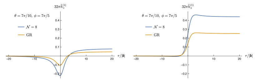
8.3 Next-to-leading order (NLO)
The NLO time-domain waveform follows from the component of section 3.4. Here we first consider the amplitude contribution. We further separate out the tail contribution from the IR finite one-loop amplitude contribution (7),
| (193) | ||||
| (194) |
We first compute which contain the contribution of . They are obtained by combining eqs. 71 and 3.4:
| (195) | ||||
| (196) |
We note that and do not correspond to the real and imaginary part of the amplitude contribution to the waveform, because the polarization vectors in these expressions are still complex. The tail contribution will be computed later in this section. We emphasize that we will only consider the amplitude contribution to the waveform, namely, the Fourier transform of in eq. 75. We will study , which is purely imaginary, in the next section.
As at leading order, we compute the integral over in by decomposing this variable in the basis of 4d vectors in eq. 182. For both GR and supergravity, it is easier to compute due to the presence of
| (197) |
Thus we can use the three delta functions in to localize the integrals over the , and variables. For fixed the integrand is now an algebraic function of . The resulting integral over is convergent and performed numerically. The background at is also subtracted at the end.
In contrast, there are only two delta functions in , which localize and . For supergravity, the integrand is a rational function in and according to section 7. Therefore, we can integrate using the residue theorem, resulting in an algebraic function of , which will be integrated numerically. For supergravity, the subtraction of background at can be done before or after the final integral since it does not affect the convergence.
However, for GR, after localizing and , the integrand contains square roots according to section 7. For this case, we still first integrate over . After some rescaling, the integral has the following generic form,
| (198) |
where is a rational function, and we have changed the variable to . Since the original integral is convergent, there are no poles at and after the change of variable. We can evaluate this integral by summing over all the residues, which leads to the final answer in eq. 198. Now if we subtract the background at , the final integral is convergent and we integrate it numerically. Unlike the previous cases, the background subtraction needs to be done before the integrals because the integral is divergent otherwise. Alternatively, if one keeps , the integration and background subtraction can be done in any order, the difference being at most some local terms in the waveform and memory.
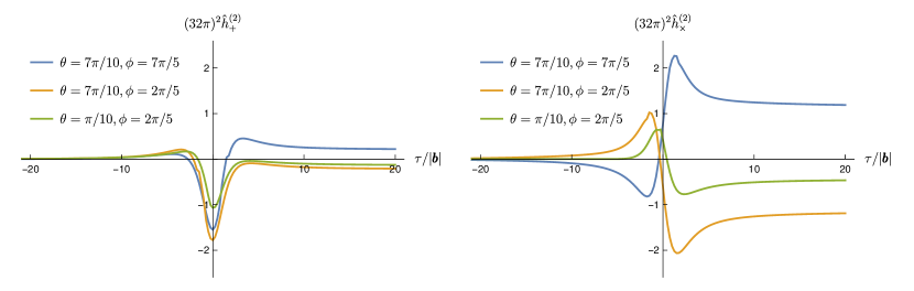
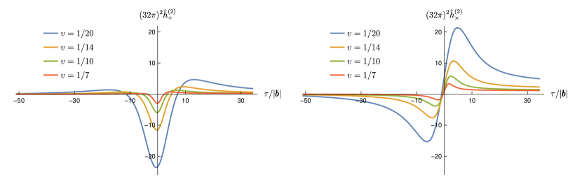
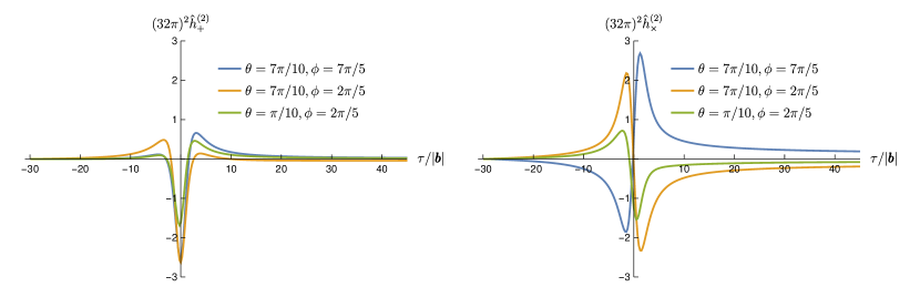
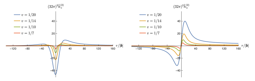
We plot the amplitude contribution to the NLO waveforms in GR observed at several angles at the spatial infinity in figure 10. In this figure, we fix the COM velocity of the two black holes to be . Then, in figure 11, we fix the observation angle to be and vary the velocities of the black holes. At low velocities, the waveforms have a much larger magnitude and are more spread out in the time domain; we may understand this intuitively by noting that at lower velocities, the two particles have a smaller minimal separation, so they experience larger accelerations and therefore radiate more. We also note that at lower velocities, we are closer to the boundary of the PM regime, which requires that be sufficiently large.
Finally, for comparison, we include in figures 12 and 13 the amplitude contribution to the NLO waveforms in supergravity. As expected, this contribution to the waveforms do not display any memory effect at NLO. At low velocities, for example, , the imaginary part exhibits a small residual at ; this is merely an artifact of our initial and final times not being infinite. We note that the profile is spread over a larger time interval and that they have a larger amplitude than the corresponding GR one. A possible explanation is that fields of the supergravity yield an additional net attractive force increasing the acceleration experienced by the two particles relative to GR.
We remark that at certain angles, the amplitude contribution displays features which, for lack of a better name, we refer to as “kinks.” For example, such kinks can be seen in figure 10 for at and . At these locations, several terms in the integrand become sharply peaked (but finite), and the resulting large values of the integral cancel over many orders of magnitude. Our numerical evaluation further suggests that more prominent kinks exist at some other angles, such as , which corresponds to an observation direction parallel to in the plane of the two incoming particles. It is unclear whether these features are merely numerical artifacts due to cancelation between large numbers, or they are physical. A definitive answer can be provided by an analytic evaluation of the waveform, which we leave for future work.
We now turn to the evaluation of the gravitational-wave tails. To this end we plug of section 8.3 into of eq. 71. As discussed in section 3.4, to evaluate the Fourier transform to the time domain in the presence of the logarithmic dependence on we simply differentiate eq. 71 with respect to . Thus,
| (199) | ||||
Since the integral is finite, we compute it directly in four dimensions. To this end we parametrize as in (182) and evaluate the integrals using the explicit -functions. Unlike eqs. (196) and (197), the logarithmic dependence on prevents the appearnce a third function. Since the integrand does not exhibit branch cuts in we evaluate this integral analytically using Cauchy’s residue theorem. The last integral, over , is evaluated numerically.
We also need to choose a value for the cutoff defining the infrared soft virtual gravitons.191919The choice of is arbitrary and the waveform is invariant under after a concurrent redefinition of the observation time, in eq. 59. Nevertheless, one needs to make a choice, which is related to the typical frequency scale at the origin of the observation time Porto:2012as . It is required to be well-inside the soft region defining the classical limit, . We may therefore set a dimensionless bound on the product of and the impact parameter , which is being the Fourier-conjugate of the momentum transfer. We will choose . Since in the classical limit and the frequency of the outgoing graviton are of the same order, we may also relate and the lowest frequency accessible to a detector. The results for GR and supergravity are plotted in figures 14, 15, 16 and 17, and we have chosen the same observation angles and velocities as before.
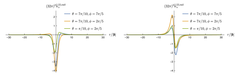
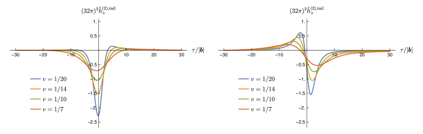
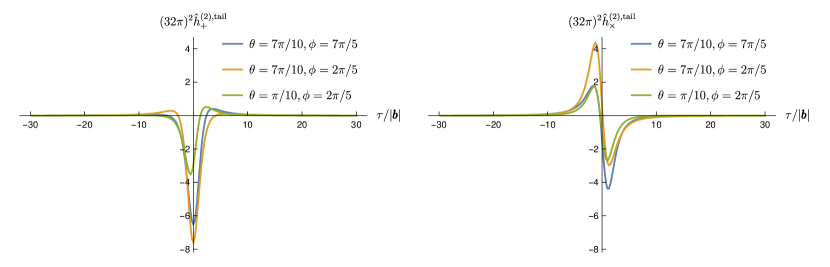
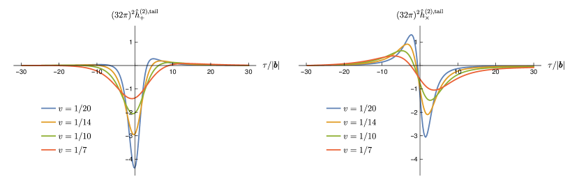
We note the absence of a memory contribution from the gravitational-wave tail, in agreement with the vanishing soft limit of the imaginary part of the one-loop five-point amplitude, as well as the close similarities of the velocity dependence of the tail and to the two gravitational-wave polarizations at fixed angle. In both contributions a higher amplitude of the wave corresponds to lower-velocity scattering, in agreement with the intuition that for fixed impact parameter lower-velocity particles experience a larger acceleration. Moreover, the angular dependence of the tail and of contributions to are also similar in shape and velocity dependence. In contrast, their contributions are quite different, cf. e.g. the right panels of figures 11 and 15. While the gravitational-wave tail contributions may be changed somewhat by varying the cutoff , a difference between and persists. It is tempting to speculate that such a difference might offer an observable signature distinguishing the gravitational-wave tail from the local-in-time effects.
9 Cut contribution
As discussed in section 3.4, the NLO waveform received two contributions: (1) from the virtual one-loop five-point amplitude and (2) from a bilinear-in- cut term shown in figure 18 whose importance was emphasized in Ref. Caron-Huot:2023vxl . In previous sections we computed the former and discussed in detail its contribution to the waveform. In this section we summarize the calculation of the latter and its contribution to the gravitational-wave memory in GR and in supergravity. We also include plots of the complete waveform.
As mentioned earlier, in the full quantum theory the cut contribution may be extracted by simply taking the cut of the virtual amplitude. In the classical limit, the matter propagators of the amplitude combine to become principal-valued (PV) propagators. Since such propagators do not exhibit a singularity, one may naively conclude that this cut vanishes. However, writing out the PV propagator as a sum two Feynman propagators reveals that the required cut is nonvanishing and the absence of the singularity of the PV propagator is due to the difference of the momenta of the two propagators being . Thus, a less naive conclusion is that the -channel cut picks out one of the two terms of the PV propagator and cancels it when subtracted from the amplitude. This cancellation was first pointed out in Ref. Caron-Huot:2023vxl .
9.1 The full waveform integrand
We computed the cut directly using the same strategy as the previous sections. Its general expression is
| (200) |
where the tree amplitudes include the momentum-conservng delta functions. Taking them to belong to the theory of interest (i.e. either GR or SG), the calculation proceeds in the standard way, by expanding in the soft limit and paying attention to the cut conditions imposed by the delta functions. As discussed in Ref. Caron-Huot:2023vxl , the classical part of the cut receives contribitions from the classical tree-level amplitudes and the second-order term in the expansion of the on-shell conditions.
To write out the result, it is convenient to introduce a new class of integrals
| (201) |
We refer the super-classical and classical part of as . After reducing the cut to a master-integral basis, the general structure of its super-classical and classical terms is
| (202) | ||||
where are superclassical contributions and and are classical. The coefficients and are related by
| (203) |
We have verified that the coefficients are such that the superclassical term cancel against those of the amplitude, in agreement with the general arguments in section 3.2. The remaining integrals cancel one of the two terms in the PV propagator, as shown in Ref. Caron-Huot:2023vxl and outlined earlier in this section.
Rather than use this cancellation, it is convenient for us to evaluate the integrals directly, for incoming and . The result for the classical part of the matrix element at one-loop order is
| (204) |
where for GR and for . The expressions of the relevant integrals are included in appendix C. The on the first line is the IR divergence, while the one on the second line has a UV origin. In both GR and , it is
| (205) |
The UV contribution is independent of the momentum transfer and corresponds to a contact interaction in impact parameter space. We will therefore discard it. The explicit expressions of the coefficients are included in two ancillary files, GR_Cut_Coeffs.m and Neq8_Cut_Coeffs.m, for GR and supergravity, respectively.
The matrix element (75) determining the waveform, which combines the virtual amplitude and the cut (bilinear-in-) contribution, is
| (206) |
where we have put back the momentum conservation delta function. Comparing with eq. 75, one can read off the expression for and . In particular, we have . Combining section 7 and the first line of eq. 204 leads to the full IR divergence of the waveform,
| (207) |
which, for the case of GR, reproduces the calculation of Ref. Caron-Huot:2023vxl .202020A possible interpretation of the IR divergence is based on the departure of the incoming trajectories from straight lines due to gravitational interactions Caron-Huot:2023vxl . However, we note that, unlike the universal Weinberg IR divergence for the amplitudes, the cut contribution is sensitive to the details of the theory through the numerical coefficient for GR and SG, respectively. In SG the IR divergence receives contributions from the other light fields of the theory. We note that this IR divergence is compatible with section 3.3 and thus can be removed by a time shift as described in section 3.3.
9.2 The complete waveform
Having computed the bilinear-in- contribution, we now proceed to complete the discussion in section 8 and assemble the NLO waveform. We first discuss the gravitational-wave memory and then the time-domain waveform.
9.2.1 Memory
As we discussed previously, the amplitude contribution to the gravitational-wave memory is given in eq. (180) and is completely determined by the real part of the virtual amplitude. The cut contributes only to the imaginary part of the matrix element and its contribution to the memory is
| (208) |
We evaluate the Fourier transforms by direct integration using the coordinate system in eq. 182 as in Cristofoli:2021vyo . The final result is
| (209) |
where and for GR and respectively. The asymptotic metric at NLO follows then from eqs. (174), (175) and (209).
We can now compare the memory contribution to the asymptotic metric with existing predictions for the GR memory Sahoo:2021ctw , which writes the universal terms in the small frequency expansion of the asymptotic metric in terms of the classical incoming and outgoing momenta. The leading soft (memory) term is
| (210) |
In this expression, the outgoing matter momenta are given in terms of the incoming momenta and the (classical) impulse; through they are
| (211) |
so becomes
| (212) |
where
| (213) | ||||
| (214) |
The tree-level and one-loop GR impulses entering section 9.2.1 were computed in Ref. Herrmann:2021tct and, in our conventions,212121The momentum transfer in Herrmann:2021tct is defined to be the opposite of ours, . This in turn implies that the impact parameter vector has the opposite orientation from ours, . are given by
| (215) |
where the transverse and longitudinal components of the impulse are
| (216) |
Upon substituting section 9.2.1 into section 9.2.1, one finds,
| (217) |
which matches the combined soft limit of the amplitude contribution (188) and the cut contribution (209) for both GR and . Therefore, we have verified that the memory given by the waveform reproduces the prediction from Ref. Sahoo:2021ctw .
9.2.2 Time-domain waveform
The evaluation of follows the same steps as those leading to the evaluation of . While the cut contribution is purely imaginary (for real polarization tensors), it contributes to both and polarizations of the gravitational wave.
Instead of plotting the cut contribution separately, we directly combine it with the amplitude contribution discussed in section 8.3 and plot the complete waveform. As in section 8.3 we will choose the scale so that . Interestingly, and as may perhaps be anticipated by comparing the scales of figures 10 and 14, for such values of the tail contribution dominates the waveform.
We assume a center-of-mass frame and equal-mass particles moving initially along the -axis. In figure 19 we show the NLO and polarizations for a selection of directions of observation specified by the polar angles and while figure 20 includes the two polarizations at fixed obervation direction but for various initial particle velocity (in units of the speed of light).
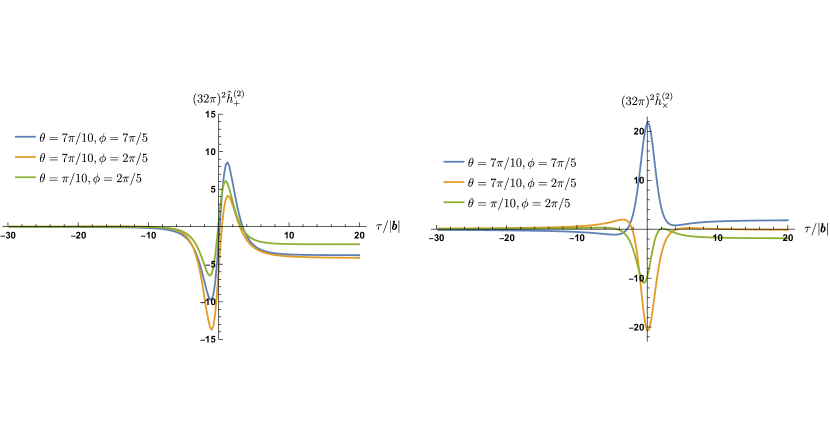
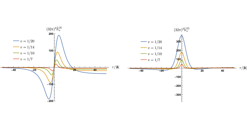
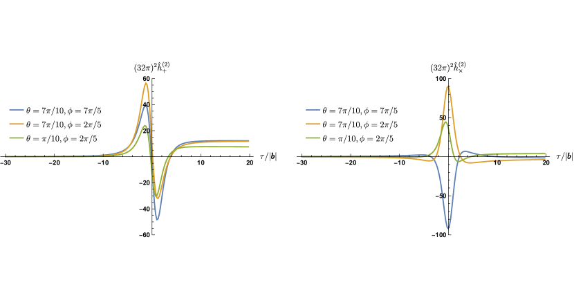
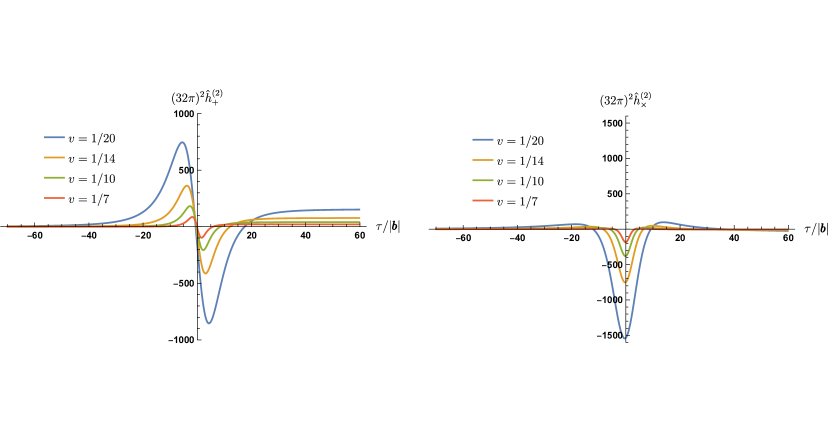
Figures 21 and 22 show the analogous plots for supergravity. We note the presence of gravitational wave memory; as discussed in section 9.2.1, it arises entirely from the cut contribution. Its analytic expression follows from section 9.2.1 upon using the SG impulses, i.e. and fixed by the on-shell condition in terms of the tree-level impulse .
10 Conclusions
The observable-based formalism Kosower:2018adc ; Cristofoli:2021vyo directly links scattering amplitudes and their cuts to observables of unbound binary systems in the classical regime. This framework naturally includes both conservative and dissipative effects, providing a means to find local observables such as the asymptotic gravitational waveform for a scattering event in addition to inclusive ones such as the impulse or the energy and angular momentum loss. With the possible exception of singular momentum configurations, they are governed by four and five-point amplitudes Cristofoli:2021jas . We examined in detail this connection for the scattering waveform and found that the exponential form of amplitudes proposed in Refs. Bern:2021dqo ; Damgaard:2021ipf implies that only (the suitably-defined) two-matter-particle-irreducible components of the amplitude can contribute to the virtual part of this observable at least through one-loop order.
We computed these parts of the four-scalar-one-graviton amplitude at one-loop order in GR with minimally-coupled scalars and in supergravity. We obtained the former using generalized unitarity, both by evaluating the classical part of the complete amplitude and by using a HEFT approach which effectively corresponds to truncating the tree amplitudes to classical order. Comparing the two results and requiring that they agree reveals that the HEFT uncut matter propagators should be interpreted as principal-valued. We obtained the integrand of the corresponding five-point one-loop amplitude in supergravity by using the double copy of the corresponding integrand in super-Yang-Mills theory and dimensional reduction. For both theories we computed directly the relevant cut contribution as well.
Upon reduction to master integrals, the five-point classical amplitudes exhibit novel features compared to their four-point counterparts. For example, the outgoing graviton momentum injects a scale in some of the scaleless (and thus vanishing) integrals in the four-point amplitude, implying that they can contribute to the five-point classical amplitude.
The one-loop master integrals are sufficiently simple so we evaluated them by direct integration for physical kinematics.222222They may also be evaluated as classical limits of the known one-loop master integrals that appear in the quantum theory. A distinguishing feature of the (2MPI part of the) classical five-point amplitude and of the cut contribution to the waveform is that they exhibit infrared-divergent phases. The structure of the amplitude’s phase divergence is governed by Weinberg’s classic result Weinberg:1965nx and the classical nature of the amplitude; we argue that at this order – and perhaps to all orders in perturbation theory – it can be absorbed as a suitable shift in the definition of the retarded time. Consequently, the observation of the gravitational waveform is sensitive only to differences of retarded times rather than the absolute time of the process. This is consistent with the basic assumption of scattering theory that observations are carried out at infinite times. We also gave a precise relation between the gravitational-wave memory and the soft limit of the corresponding scattering amplitude, along the lines of Refs. Strominger:2014pwa ; Sahoo:2021ctw , demonstrating a close relation between the amplitude’s contribution to the memory and the scattering angle to at least . Interestingly, this implies that the amplitude’s contribution to the gravitational-wave memory vanishes at for half-BPS black holes in supergravity, which is confirmed by the explicit calculation. The cut however yields a nonzero memory both in general relativity and in supergravity.
Even though our results are analytic in frequency and momentum space as well as in time-momentum space, we resorted to numerical integration to evaluate the one-dimensional integral completing the transformation to time-impact parameter space. A complete analytic evaluation of the waveform, which we leave for future work, would involve obtaining an analytic expression for this last one-dimensional integral. The result would resolve certain numerical features that we encountered at special observation angles and would open the door to the evaluation of interesting inclusive and local observables, such as the energy and angular momentum loss at and the radiated energy spectrum through traditional general relativity methods Bonga:2018gzr ; Thorne:1980ru ; DeWitt:2011nnj ; Peters:1964zz . The classical one-loop five-point amplitude constructed here allows the computation of inclusive quantities at 4PM order through the KMOC formalism, along the lines of the 3PM calculations of Refs. Herrmann:2021lqe ; Herrmann:2021tct ; Manohar:2022dea .
While the next-to-leading order is the current state of the art for relativistic scattering waveforms, it is natural to think about higher orders. The experience with -extended supergravity loop calculations Bern:2009kd ; Carrasco:2011mn ; Bern:2013uka ; Bern:2014sna ; Bern:2017ucb ; Bern:2018jmv suggests that the construction of the relevant classical integrand through double copy and generalized unitarity should scale well to higher orders and the results will provide tests of the HEFT approach to classical amplitudes beyond those already available. We expect, however, that the evaluation of the resulting master integrals will benefit from advanced techniques such as differential equations and method of regions, as was done for the full quantum two-loop five-point amplitude of supergravity in Ref. Abreu:2019rpt .
The current approach to analytic and semi-analytic binary inspiral waveforms makes use of the effective one-body formalism Buonanno:1998gg ; Buonanno:2000ef , whose input is an off-shell binary Hamiltonian and radiation reaction forces. It would be interesting to identify features of gravitational waveforms that can be analytically continued between bound and unbound systems, in analogy with inclusive observables discussed in Refs. Kalin:2019rwq ; Kalin:2019inp ; Cho:2021arx . We may expect that a detailed understanding of the analytic structure of the waveforms, both in the bound and unbound case, will be important.
Acknowledgements.
We thank A. Elkhidir, D. O’Connell, M. Sergola, I. Vazquez-Holm, and A. Brandhuber, G. Brown, G. Chen, S. De Angelis, J. Gowdy, G. Travaglini and L. Bohnenblust, H. Ita, M. Kraus and J. Schlenk for coordination on ongoing work. We also thank N. Arkani-Hamed, R. Akhoury, J. Berman, R. Britto, T. Damour, S. DeAngelis, L. Dixon, H. Elvang, S. Mizera, A. Sen, C.-H. Shen and G. Sterman for stimulating discussions. RR and FT also thank Z. Bern, E. Herrmann, J. Parra-Martinez, M. Ruf, C.-H. Shen, and M. Zeng for collaboration on related topics, and especially M. Ruf for providing valuable comments on our draft. RR and FT would like to thank the Kavli Institute for Theoretical Physics at the University of California, Santa Barbara, for hospitality during the program “High-Precision Gravitational Waves”. Their research there was supported in part by the National Science Foundation under Grant No. NSF PHY-1748958. AH is supported by a Rackham Predoctoral Fellowship from the University of Michigan. RR and FT are supported by the U.S. Department of Energy (DOE) under award number DE-SC00019066.Appendix A Self-consistency of HEFT
In this appendix, we focus on terms containing two-matter-particle cuts on which the HEFT integrand factorizes into lower point HEFT integrands. We argue such terms require quantum information about the HEFT tree amplitudes used in the unitarity construction.
We will use the counting as introduced in eq. 2. Consider a cut of a four-scalar amplitude containing HEFT tree amplitudes, each with internal gravitons external gravitons, and scalars; call and respectively the total number of internal and external gravitons, and the total number of internal scalars. Restoring the integration measure and the matter and graviton propagators, this cut scales as
| (218) |
where we have used eq. 3 and the loop number . This cut scales classically if
| (219) |
Consistency requires that if we cut any line the result should still scale classically. Let us consider cutting a pair of matter lines. The resulting eight-scalar amplitude scales as
| (220) |
Here we have isolated the classical scaling of an eight-scalar amplitude. If the graph remains connected, then we remove two matter propagators and two integral measures from eq. 218, which leads to . On the other hand, if the graph is now disconnected, then we only need to remove two matter propagators and one integral measure instead, which leads to . Thus, if – i.e. if the cut of the eight-scalar amplitude is connected – then it has classical scaling upon use of eq. 219 and the truncation to classical order is iteratively consistent. In contrast, if – i.e. if the cut of the eight-scalar amplitude is disconnected – the cut is suppressed by , which means that the disconnected components contain quantum contributions.
Repeating the calculation above for any pair of matter lines, it follows that any 2MPR contribution constructible by generalized unitarity with a classical scaling requires quantum information about some amplitude contributing to it. Since the HEFT approach prescribes that tree amplitudes be truncated to classical orders, the scaling of 2MPR diagrams and cuts with classical vertices is super-classical, with one factor of for each present two-matter-particle cut. On the other hand, if we explicitly include some quantum operators in the Lagrangian and keep higher-order terms in the HEFT tree amplitudes, we will get classical 2MPR contributions. Again, the above argument only applies to two-matter-particle cuts on which the HEFT integrand factorizes into lower point integrands.
Appendix B Evaluating box master integrals
In this appendix, we derive all the box master integrals listed in section 6.2. We will repeatedly use the bubble integral with a cut matter propagator and a generic propagator in ,
| (221) |
where is a generic vector.
B.1
We first compute the box integral with three graviton propagators,
| (222) |
where we have introduced a Feynman parameter to combine the two massless propagators and into a single propagator. We next use an IBP identity to reduce the double propagator ,
| (223) |
The integral in the last line is finite in ,232323One can show this by using for the integral. The remaining integral is convergent. such that the prefactor makes this term only contribute to order. Thus both the IR divergence and the finite part are given by the first term of section B.1,
| (224) | ||||
The prescription suggests the analytic continuation for and , which gives
| (225) |
The result agrees with eq. 146 in the main text.
B.2
We next consider the box integrals with one uncut matter propagator. We start with
| (226) |
where we have used the eq. 138 to combine and . The IBP identity can reduce the double propagator
| (227) |
The integral proportional to contributes to order, for a reason similar to the discussion below section B.1. Now using eq. 221 for the bubble integral in the second line of section B.2, we get the IR divergence and the finite part of this integral,
| (228) |
Here we can omit the prescription in because the argument is positive. To compute , we first redefine the loop momentum to flip the sign of ,
| (229) |
We can directly obtain the result of this integral by sending in section B.2 while preserving the sign of ,
| (230) |
Therefore, the combination is free of IR divergences,
| (231) |
which reproduces eq. 147a.
B.3
We apply the same strategy to compute the last set of box integrals,
| (232) |
The only difference here is that the combination is now complex, with the imaginary part given by further cutting . Starting with , we first apply eq. 138 to combine and , followed by using an IBP identity to get,
| (233) |
where and are defined as
| (234) |
Similar to eq. 229, we can rewrite as
| (235) |
where . Therefore, we have
| (236) |
such that we only need to compute the combination and .
If we use eq. 221 with to integrate out the bubble in , we will find that the resulting integral is divergent at . However, by taking the difference , we get a finite result since the range of gets truncated. Interestingly, the result is proportional to the triangle integral (143),
| (237) |
To compute , we introduce another Feynman parameter and perform the integral in . The result is finite due to the same truncation on the range of ,
| (238) |
such that in . Therefore, we have reproduced eq. 147b,
| (239) |
B.4
We first use the same Feynman parameterization as in eq. 222 to bring together the two massless propagators,
| (240) |
The resultant double propagator is then reduced by the IBP relation,
| (241) |
where is a quadratic polynomial in ,
| (242) |
Under the principal value combination , the first integral in section B.4 is doubled while the second integral is finite in , which only contributes to due to the prefactor. We can now reproduce eq. 148 through a direct integration,
| (243) | ||||
Appendix C Master integrals determining the cut contribution
In this appendix, we list all the double-cut master integrals,
| (244) |
necessary for Sec. 9.1. Due to the two delta functions, the dimension of the integral is reduced by two and the integrals are easy to evaluate directly using the same computation strategies as appendix B. Therefore, we simply summarize the results below:
| (245) |
| (246) |
| (247) |
| (250) | ||||
| (251) |
| (254) | ||||
| (255) |
Some of the integrals listed here have also been evaluated in Ref. Caron-Huot:2023vxl .
References
- (1) LIGO Scientific, Virgo, KAGRA collaboration, GWTC-3: Compact Binary Coalescences Observed by LIGO and Virgo During the Second Part of the Third Observing Run, 2111.03606.
- (2) A. Buonanno and T. Damour, Effective one-body approach to general relativistic two-body dynamics, Phys. Rev. D 59 (1999) 084006 [gr-qc/9811091].
- (3) T. Damour, P. Jaranowski and G. Schaefer, On the determination of the last stable orbit for circular general relativistic binaries at the third postNewtonian approximation, Phys. Rev. D 62 (2000) 084011 [gr-qc/0005034].
- (4) A. Buonanno and T. Damour, Transition from inspiral to plunge in binary black hole coalescences, Phys. Rev. D 62 (2000) 064015 [gr-qc/0001013].
- (5) T. Damour, Coalescence of two spinning black holes: an effective one-body approach, Phys. Rev. D 64 (2001) 124013 [gr-qc/0103018].
- (6) T. Damour and A. Nagar, New effective-one-body description of coalescing nonprecessing spinning black-hole binaries, Phys. Rev. D 90 (2014) 044018 [1406.6913].
- (7) F. Pretorius, Evolution of binary black hole spacetimes, Phys. Rev. Lett. 95 (2005) 121101 [gr-qc/0507014].
- (8) F. Pretorius, Binary Black Hole Coalescence, 0710.1338.
- (9) L. Blanchet, Gravitational Radiation from Post-Newtonian Sources and Inspiralling Compact Binaries, Living Rev. Rel. 17 (2014) 2 [1310.1528].
- (10) G. Schäfer and P. Jaranowski, Hamiltonian formulation of general relativity and post-Newtonian dynamics of compact binaries, Living Rev. Rel. 21 (2018) 7 [1805.07240].
- (11) W.D. Goldberger and I.Z. Rothstein, An Effective field theory of gravity for extended objects, Phys. Rev. D 73 (2006) 104029 [hep-th/0409156].
- (12) W.D. Goldberger and I.Z. Rothstein, Towers of Gravitational Theories, Gen. Rel. Grav. 38 (2006) 1537 [hep-th/0605238].
- (13) W.D. Goldberger and A. Ross, Gravitational radiative corrections from effective field theory, Phys. Rev. D 81 (2010) 124015 [0912.4254].
- (14) R.A. Porto, A. Ross and I.Z. Rothstein, Spin induced multipole moments for the gravitational wave amplitude from binary inspirals to 2.5 Post-Newtonian order, JCAP 09 (2012) 028 [1203.2962].
- (15) L. Blanchet and B.S. Sathyaprakash, Detecting the tail effect in gravitational wave experiments, Phys. Rev. Lett. 74 (1995) 1067.
- (16) R.A. Porto, The effective field theorist’s approach to gravitational dynamics, Phys. Rept. 633 (2016) 1 [1601.04914].
- (17) M. Levi, Effective Field Theories of Post-Newtonian Gravity: A comprehensive review, Rept. Prog. Phys. 83 (2020) 075901 [1807.01699].
- (18) M. Khalil, A. Buonanno, J. Steinhoff and J. Vines, Energetics and scattering of gravitational two-body systems at fourth post-Minkowskian order, Phys. Rev. D 106 (2022) 024042 [2204.05047].
- (19) S.J. Kovacs and K.S. Thorne, The Generation of Gravitational Waves. 1. Weak-field sources, Astrophys. J. 200 (1975) 245.
- (20) R.J. Crowley and K.S. Thorne, The Generation of Gravitational Waves. 2. The Postlinear Formalism Revisited, Astrophys. J. 215 (1977) 624.
- (21) S.J. Kovacs and K.S. Thorne, The Generation of Gravitational Waves. 3. Derivation of Bremsstrahlung Formulas, Astrophys. J. 217 (1977) 252.
- (22) S.J. Kovacs and K.S. Thorne, The Generation of Gravitational Waves. 4. Bremsstrahlung, Astrophys. J. 224 (1978) 62.
- (23) D. Amati, M. Ciafaloni and G. Veneziano, Higher Order Gravitational Deflection and Soft Bremsstrahlung in Planckian Energy Superstring Collisions, Nucl. Phys. B 347 (1990) 550.
- (24) M. Ciafaloni, D. Colferai and G. Veneziano, Infrared features of gravitational scattering and radiation in the eikonal approach, Phys. Rev. D 99 (2019) 066008 [1812.08137].
- (25) T. Damour, Radiative contribution to classical gravitational scattering at the third order in , Phys. Rev. D 102 (2020) 124008 [2010.01641].
- (26) G. Kälin and R.A. Porto, Post-Minkowskian Effective Field Theory for Conservative Binary Dynamics, JHEP 11 (2020) 106 [2006.01184].
- (27) G. Kälin, Z. Liu and R.A. Porto, Conservative Dynamics of Binary Systems to Third Post-Minkowskian Order from the Effective Field Theory Approach, Phys. Rev. Lett. 125 (2020) 261103 [2007.04977].
- (28) C. Dlapa, G. Kälin, Z. Liu and R.A. Porto, Dynamics of binary systems to fourth Post-Minkowskian order from the effective field theory approach, Phys. Lett. B 831 (2022) 137203 [2106.08276].
- (29) E. Herrmann, J. Parra-Martinez, M.S. Ruf and M. Zeng, Radiative classical gravitational observables at (G3) from scattering amplitudes, JHEP 10 (2021) 148 [2104.03957].
- (30) M.M. Riva and F. Vernizzi, Radiated momentum in the post-Minkowskian worldline approach via reverse unitarity, JHEP 11 (2021) 228 [2110.10140].
- (31) S. Mougiakakos, M.M. Riva and F. Vernizzi, Gravitational Bremsstrahlung with Tidal Effects in the Post-Minkowskian Expansion, Phys. Rev. Lett. 129 (2022) 121101 [2204.06556].
- (32) M.M. Riva, F. Vernizzi and L.K. Wong, Gravitational bremsstrahlung from spinning binaries in the post-Minkowskian expansion, Phys. Rev. D 106 (2022) 044013 [2205.15295].
- (33) A.V. Manohar, A.K. Ridgway and C.-H. Shen, Radiated Angular Momentum and Dissipative Effects in Classical Scattering, Phys. Rev. Lett. 129 (2022) 121601 [2203.04283].
- (34) G.U. Jakobsen, G. Mogull, J. Plefka and B. Sauer, All things retarded: radiation-reaction in worldline quantum field theory, JHEP 10 (2022) 128 [2207.00569].
- (35) G.U. Jakobsen, G. Mogull, J. Plefka and J. Steinhoff, Classical Gravitational Bremsstrahlung from a Worldline Quantum Field Theory, Phys. Rev. Lett. 126 (2021) 201103 [2101.12688].
- (36) G.U. Jakobsen, G. Mogull, J. Plefka and J. Steinhoff, Gravitational Bremsstrahlung and Hidden Supersymmetry of Spinning Bodies, Phys. Rev. Lett. 128 (2022) 011101 [2106.10256].
- (37) G. Kälin, J. Neef and R.A. Porto, Radiation-reaction in the Effective Field Theory approach to Post-Minkowskian dynamics, JHEP 01 (2023) 140 [2207.00580].
- (38) G. Kälin and R.A. Porto, From Boundary Data to Bound States, JHEP 01 (2020) 072 [1910.03008].
- (39) G. Kälin and R.A. Porto, From boundary data to bound states. Part II. Scattering angle to dynamical invariants (with twist), JHEP 02 (2020) 120 [1911.09130].
- (40) D. Bini, T. Damour and A. Geralico, Sixth post-Newtonian nonlocal-in-time dynamics of binary systems, Phys. Rev. D 102 (2020) 084047 [2007.11239].
- (41) G. Cho, G. Kälin and R.A. Porto, From boundary data to bound states. Part III. Radiative effects, JHEP 04 (2022) 154 [2112.03976].
- (42) D.A. Kosower, B. Maybee and D. O’Connell, Amplitudes, Observables, and Classical Scattering, JHEP 02 (2019) 137 [1811.10950].
- (43) A. Cristofoli, R. Gonzo, D.A. Kosower and D. O’Connell, Waveforms from amplitudes, Phys. Rev. D 106 (2022) 056007 [2107.10193].
- (44) Z. Bern, L.J. Dixon, D.C. Dunbar and D.A. Kosower, One loop -point gauge theory amplitudes, unitarity and collinear limits, Nucl. Phys. B425 (1994) 217 [hep-ph/9403226].
- (45) Z. Bern and A.G. Morgan, Massive loop amplitudes from unitarity, Nucl. Phys. B467 (1996) 479 [hep-ph/9511336].
- (46) Z. Bern, L.J. Dixon, D.C. Dunbar and D.A. Kosower, Fusing gauge theory tree amplitudes into loop amplitudes, Nucl. Phys. B435 (1995) 59 [hep-ph/9409265].
- (47) Z. Bern, L.J. Dixon and D.A. Kosower, One loop amplitudes for e+ e- to four partons, Nucl. Phys. B 513 (1998) 3 [hep-ph/9708239].
- (48) R. Britto, F. Cachazo and B. Feng, Generalized unitarity and one-loop amplitudes in N=4 super-Yang-Mills, Nucl. Phys. B 725 (2005) 275 [hep-th/0412103].
- (49) Z. Bern, J.J.M. Carrasco, H. Johansson and D.A. Kosower, Maximally supersymmetric planar Yang-Mills amplitudes at five loops, Phys. Rev. D 76 (2007) 125020 [0705.1864].
- (50) Z. Bern, J.J.M. Carrasco and H. Johansson, New relations for gauge-theory amplitudes, Phys. Rev. D78 (2008) 085011 [0805.3993].
- (51) Z. Bern, J.J.M. Carrasco and H. Johansson, Perturbative quantum gravity as a double copy of gauge theory, Phys. Rev. Lett. 105 (2010) 061602 [1004.0476].
- (52) H. Kawai, D.C. Lewellen and S.H.H. Tye, A relation between tree amplitudes of closed and open strings, Nucl. Phys. B269 (1986) 1.
- (53) A.V. Kotikov, Differential equations method: New technique for massive Feynman diagrams calculation, Phys. Lett. B 254 (1991) 158.
- (54) Z. Bern, L.J. Dixon and D.A. Kosower, Dimensionally regulated pentagon integrals, Nucl. Phys. B 412 (1994) 751 [hep-ph/9306240].
- (55) E. Remiddi, Differential equations for Feynman graph amplitudes, Nuovo Cim. A 110 (1997) 1435 [hep-th/9711188].
- (56) T. Gehrmann and E. Remiddi, Differential equations for two loop four point functions, Nucl. Phys. B 580 (2000) 485 [hep-ph/9912329].
- (57) K.G. Chetyrkin and F.V. Tkachov, Integration by Parts: The Algorithm to Calculate beta Functions in 4 Loops, Nucl. Phys. B 192 (1981) 159.
- (58) A.V. Smirnov, Algorithm FIRE – Feynman Integral REduction, JHEP 10 (2008) 107 [0807.3243].
- (59) A.V. Smirnov and F.S. Chuharev, FIRE6: Feynman Integral REduction with Modular Arithmetic, Comput. Phys. Commun. 247 (2020) 106877 [1901.07808].
- (60) S. Caron-Huot, M. Giroux, H.S. Hannesdottir and S. Mizera, What can be measured asymptotically?, 2308.02125.
- (61) Z. Bern, J. Parra-Martinez, R. Roiban, M.S. Ruf, C.-H. Shen, M.P. Solon et al., Scattering Amplitudes and Conservative Binary Dynamics at , Phys. Rev. Lett. 126 (2021) 171601 [2101.07254].
- (62) P.H. Damgaard, L. Plante and P. Vanhove, On an exponential representation of the gravitational S-matrix, JHEP 11 (2021) 213 [2107.12891].
- (63) A. Brandhuber, G. Chen, G. Travaglini and C. Wen, A new gauge-invariant double copy for heavy-mass effective theory, JHEP 07 (2021) 047 [2104.11206].
- (64) A. Brandhuber, G. Chen, G. Travaglini and C. Wen, Classical gravitational scattering from a gauge-invariant double copy, JHEP 10 (2021) 118 [2108.04216].
- (65) N. Arkani-Hamed, F. Cachazo and J. Kaplan, What is the Simplest Quantum Field Theory?, JHEP 09 (2010) 016 [0808.1446].
- (66) S. Caron-Huot and Z. Zahraee, Integrability of Black Hole Orbits in Maximal Supergravity, JHEP 07 (2019) 179 [1810.04694].
- (67) C.R. Mafra and O. Schlotterer, Towards one-loop SYM amplitudes from the pure spinor BRST cohomology, Fortsch. Phys. 63 (2015) 105 [1410.0668].
- (68) S. He, O. Schlotterer and Y. Zhang, New BCJ representations for one-loop amplitudes in gauge theories and gravity, Nucl. Phys. B 930 (2018) 328 [1706.00640].
- (69) S. Weinberg, Infrared photons and gravitons, Phys. Rev. 140 (1965) B516.
- (70) A. Brandhuber, G.R. Brown, G. Chen, S. De Angelis, J. Gowdy and G. Travaglini, One-loop Gravitational Bremsstrahlung and Waveforms from a Heavy-Mass Effective Field Theory, 2303.06111.
- (71) A. Elkhidir, D. O’Connell, M. Sergola and I.A. Vazquez-Holm, Radiation and Reaction at One Loop, 2303.06211.
- (72) C. Cheung, I.Z. Rothstein and M.P. Solon, From Scattering Amplitudes to Classical Potentials in the Post-Minkowskian Expansion, Phys. Rev. Lett. 121 (2018) 251101 [1808.02489].
- (73) Z. Bern, C. Cheung, R. Roiban, C.-H. Shen, M.P. Solon and M. Zeng, Scattering Amplitudes and the Conservative Hamiltonian for Binary Systems at Third Post-Minkowskian Order, Phys. Rev. Lett. 122 (2019) 201603 [1901.04424].
- (74) Z. Bern, C. Cheung, R. Roiban, C.-H. Shen, M.P. Solon and M. Zeng, Black Hole Binary Dynamics from the Double Copy and Effective Theory, JHEP 10 (2019) 206 [1908.01493].
- (75) A. Luna, I. Nicholson, D. O’Connell and C.D. White, Inelastic Black Hole Scattering from Charged Scalar Amplitudes, JHEP 03 (2018) 044 [1711.03901].
- (76) M. Beneke and V.A. Smirnov, Asymptotic expansion of Feynman integrals near threshold, Nucl. Phys. B 522 (1998) 321 [hep-ph/9711391].
- (77) H. Georgi, An Effective Field Theory for Heavy Quarks at Low-energies, Phys. Lett. B 240 (1990) 447.
- (78) M.E. Luke and A.V. Manohar, Reparametrization invariance constraints on heavy particle effective field theories, Phys. Lett. B 286 (1992) 348 [hep-ph/9205228].
- (79) M. Neubert, Heavy quark symmetry, Phys. Rept. 245 (1994) 259 [hep-ph/9306320].
- (80) A.V. Manohar and M.B. Wise, Heavy quark physics, vol. 10 (2000).
- (81) P.H. Damgaard, K. Haddad and A. Helset, Heavy Black Hole Effective Theory, JHEP 11 (2019) 070 [1908.10308].
- (82) R. Aoude, K. Haddad and A. Helset, On-shell heavy particle effective theories, JHEP 05 (2020) 051 [2001.09164].
- (83) K. Haddad and A. Helset, The double copy for heavy particles, Phys. Rev. Lett. 125 (2020) 181603 [2005.13897].
- (84) R. Akhoury, R. Saotome and G. Sterman, High Energy Scattering in Perturbative Quantum Gravity at Next to Leading Power, Phys. Rev. D 103 (2021) 064036 [1308.5204].
- (85) D.A. Kosower, R. Monteiro and D. O’Connell, The SAGEX Review on Scattering Amplitudes, Chapter 14: Classical Gravity from Scattering Amplitudes, 2203.13025.
- (86) E. Newman and R. Penrose, An Approach to gravitational radiation by a method of spin coefficients, J. Math. Phys. 3 (1962) 566.
- (87) E. Herrmann, J. Parra-Martinez, M.S. Ruf and M. Zeng, Gravitational Bremsstrahlung from Reverse Unitarity, Phys. Rev. Lett. 126 (2021) 201602 [2101.07255].
- (88) C. Anastasiou and K. Melnikov, Higgs boson production at hadron colliders in NNLO QCD, Nucl. Phys. B 646 (2002) 220 [hep-ph/0207004].
- (89) C. Anastasiou, L.J. Dixon and K. Melnikov, NLO Higgs boson rapidity distributions at hadron colliders, Nucl. Phys. B Proc. Suppl. 116 (2003) 193 [hep-ph/0211141].
- (90) C. Anastasiou, L.J. Dixon, K. Melnikov and F. Petriello, Dilepton rapidity distribution in the Drell-Yan process at NNLO in QCD, Phys. Rev. Lett. 91 (2003) 182002 [hep-ph/0306192].
- (91) T. Kinoshita, Mass singularities of Feynman amplitudes, J. Math. Phys. 3 (1962) 650.
- (92) T.D. Lee and M. Nauenberg, Degenerate Systems and Mass Singularities, Phys. Rev. 133 (1964) B1549.
- (93) P.A.M. Dirac, Gauge invariant formulation of quantum electrodynamics, Can. J. Phys. 33 (1955) 650.
- (94) P.P. Kulish and L.D. Faddeev, Asymptotic conditions and infrared divergences in quantum electrodynamics, Theor. Math. Phys. 4 (1970) 745.
- (95) G. Grammer, Jr. and D.R. Yennie, Improved treatment for the infrared divergence problem in quantum electrodynamics, Phys. Rev. D 8 (1973) 4332.
- (96) J. Ware, R. Saotome and R. Akhoury, Construction of an asymptotic S matrix for perturbative quantum gravity, JHEP 10 (2013) 159 [1308.6285].
- (97) V. Chung, Infrared Divergence in Quantum Electrodynamics, Phys. Rev. 140 (1965) B1110.
- (98) A. Cristofoli, R. Gonzo, N. Moynihan, D. O’Connell, A. Ross, M. Sergola et al., The Uncertainty Principle and Classical Amplitudes, 2112.07556.
- (99) R. Britto, R. Gonzo and G.R. Jehu, Graviton particle statistics and coherent states from classical scattering amplitudes, JHEP 03 (2022) 214 [2112.07036].
- (100) Z. Bern, J. Parra-Martinez, R. Roiban, M.S. Ruf, C.-H. Shen, M.P. Solon et al., Scattering Amplitudes, the Tail Effect, and Conservative Binary Dynamics at O(G4), Phys. Rev. Lett. 128 (2022) 161103 [2112.10750].
- (101) L. Blanchet and T. Damour, Hereditary effects in gravitational radiation, Phys. Rev. D 46 (1992) 4304.
- (102) L. Blanchet and G. Schaefer, Gravitational wave tails and binary star systems, Class. Quant. Grav. 10 (1993) 2699.
- (103) J.J.M. Carrasco and I.A. Vazquez-Holm, Extracting Einstein from the loop-level double-copy, JHEP 11 (2021) 088 [2108.06798].
- (104) D. Kosmopoulos, Simplifying D-dimensional physical-state sums in gauge theory and gravity, Phys. Rev. D 105 (2022) 056025 [2009.00141].
- (105) A. Koemans Collado, P. Di Vecchia and R. Russo, Revisiting the second post-Minkowskian eikonal and the dynamics of binary black holes, Phys. Rev. D 100 (2019) 066028 [1904.02667].
- (106) Z. Bern, L.J. Dixon and D.A. Kosower, Two-loop g — gg splitting amplitudes in QCD, JHEP 08 (2004) 012 [hep-ph/0404293].
- (107) J. Parra-Martinez, M.S. Ruf and M. Zeng, Extremal black hole scattering at : graviton dominance, eikonal exponentiation, and differential equations, JHEP 11 (2020) 023 [2005.04236].
- (108) G. Passarino and M.J.G. Veltman, One Loop Corrections for e+ e- Annihilation Into mu+ mu- in the Weinberg Model, Nucl. Phys. B 160 (1979) 151.
- (109) N.E.J. Bjerrum-Bohr, D.C. Dunbar, H. Ita, W.B. Perkins and K. Risager, The No-Triangle Hypothesis for N=8 Supergravity, JHEP 12 (2006) 072 [hep-th/0610043].
- (110) W.L. van Neerven and J.A.M. Vermaseren, LARGE LOOP INTEGRALS, Phys. Lett. B 137 (1984) 241.
- (111) Z. Bern, L.J. Dixon and D.A. Kosower, Dimensionally regulated one loop integrals, Phys. Lett. B 302 (1993) 299 [hep-ph/9212308].
- (112) T. Damour, Gravitational scattering, post-Minkowskian approximation and Effective One-Body theory, Phys. Rev. D 94 (2016) 104015 [1609.00354].
- (113) T. Damour, High-energy gravitational scattering and the general relativistic two-body problem, Phys. Rev. D 97 (2018) 044038 [1710.10599].
- (114) B. Sahoo and A. Sen, Classical soft graviton theorem rewritten, JHEP 01 (2022) 077 [2105.08739].
- (115) A. Strominger and A. Zhiboedov, Gravitational Memory, BMS Supertranslations and Soft Theorems, JHEP 01 (2016) 086 [1411.5745].
- (116) B. Bonga and E. Poisson, Coulombic contribution to angular momentum flux in general relativity, Phys. Rev. D 99 (2019) 064024 [1808.01288].
- (117) K.S. Thorne, Multipole Expansions of Gravitational Radiation, Rev. Mod. Phys. 52 (1980) 299.
- (118) B. DeWitt, Bryce DeWitt’s Lectures on Gravitation, vol. 826, Springer (2011), 10.1007/978-3-540-36911-0.
- (119) P.C. Peters, Gravitational Radiation and the Motion of Two Point Masses, Phys. Rev. 136 (1964) B1224.
- (120) Z. Bern, J.J. Carrasco, L.J. Dixon, H. Johansson and R. Roiban, The Ultraviolet Behavior of N=8 Supergravity at Four Loops, Phys. Rev. Lett. 103 (2009) 081301 [0905.2326].
- (121) J.J.M. Carrasco and H. Johansson, Five-Point Amplitudes in N=4 Super-Yang-Mills Theory and N=8 Supergravity, Phys. Rev. D 85 (2012) 025006 [1106.4711].
- (122) Z. Bern, S. Davies, T. Dennen, A.V. Smirnov and V.A. Smirnov, Ultraviolet Properties of N=4 Supergravity at Four Loops, Phys. Rev. Lett. 111 (2013) 231302 [1309.2498].
- (123) Z. Bern, S. Davies and T. Dennen, Enhanced ultraviolet cancellations in supergravity at four loops, Phys. Rev. D 90 (2014) 105011 [1409.3089].
- (124) Z. Bern, J.J.M. Carrasco, W.-M. Chen, H. Johansson, R. Roiban and M. Zeng, Five-loop four-point integrand of supergravity as a generalized double copy, Phys. Rev. D 96 (2017) 126012 [1708.06807].
- (125) Z. Bern, J.J. Carrasco, W.-M. Chen, A. Edison, H. Johansson, J. Parra-Martinez et al., Ultraviolet Properties of Supergravity at Five Loops, Phys. Rev. D 98 (2018) 086021 [1804.09311].
- (126) S. Abreu, L.J. Dixon, E. Herrmann, B. Page and M. Zeng, The two-loop five-point amplitude in = 8 supergravity, JHEP 03 (2019) 123 [1901.08563].