First Observation of Chromospheric Waves in a Sunspot by DKIST/ViSP: The Anatomy of an Umbral Flash

Abstract

The Visible Spectro-Polarimeter (ViSP) of the NSF Daniel K. Inouye Solar Telescope (DKIST) collected its Science Verification data on May 7-8, 2021. The instrument observed multiple layers of a sunspot atmosphere simultaneously, in passbands of Ca II 397 nm (H-line), Fe I 630 nm, and Ca II 854 nm, scanning the region with a spatial sampling of 0.041″ and average temporal cadence of 7.76 seconds, for an 38.8 minute duration. The slit moves southward across the plane-of-the-sky at 3.83 km/s. The spectropolarimetric scans exhibit prominent oscillatory ‘ridge’ structures which lie nearly perpendicular to the direction of slit motion (north to south). These ridges are visible in maps of line intensity, central wavelength, line width, and both linear and circular polarizations. Contemporaneous Atmospheric Imaging Assembly observations indicate these ridges are purely temporal in character and likely attributed to the familiar chromospheric 3-minute umbral oscillations.

We observe in detail a steady umbral flash near the center of the sunspot umbra. Although bad seeing limited the spatial resolution, the unique high signal-to-noise data enable us to estimate the shock Mach numbers (${\approx}\,2$), propagation speeds (${\approx}\,9$ km/s), and their impact on the longitudinal magnetic field ($\Delta B\approx 50$ G), gas pressure, and temperature ($\Delta T/T\approx 0.1$) of the subshocks over 30 seconds. We also find evidence for rarefaction waves situated between neighboring wave-train shocks. The Ca II 854 nm line width is fairly steady throughout the umbral flash except for a sharp 1.5 km/s dip immediately before, and comparable spike immediately after, the passage of the shock front. This zig-zag in line width is centered on the subshock and extends over 0.4″.

1 Introduction

Well over half a century since their discovery by Beckers & Tallant (1969), Schultz & White (1974), our interest in umbral flashes continues unabated. They remain one of the most striking dynamical chromospheric phenomena with roots that extend deep into the umbral photosphere and possibly as far as the subsurface magnetoconvection. They span numerous density scale heights and couple distinct atmospheric layers. They provide a means to deliver mechanical energy to the optically-thin chromosphere, transition region, and lower corona. The extensive monographs and reviews by Thomas & Weiss (2012), Weiss & Proctor (2014), and Khomenko & Collados (2015) provide an exhaustive summary and analysis of the research on umbral flashes through the first decade of the 21st Century. For more recent efforts, from both observational and theoretical perspectives, one should consult, e.g., Madsen et al. (2015), Löhner-Böttcher (2016), Song et al. (2017), Kuźma et al. (2017a), Kuźma et al. (2017b), Felipe et al. (2018), Houston et al. (2018), Stangalini et al. (2018), Joshi & de la Cruz Rodríguez (2018), Anan et al. (2019a), Bose et al. (2019), Henriques et al. (2020), Houston et al. (2020), Yurchyshyn et al. (2020), Stangalini et al. (2021a), Stangalini et al. (2021b), Felipe et al. (2021), Sadykov et al. (2021), Snow & Hillier (2021), and Molnar et al. (2021). The following earlier papers are valuable and particularly germane to what follows: Lites (1992), Centeno et al. (2006), Pietarila et al. (2006), Pietarila et al. (2007), Centeno et al. (2009), Bard & Carlsson (2010), and Felipe et al. (2014).

The present contribution to the subject adds to this body of knowledge by providing a unique high-spatial, spectral, and temporal resolution glimpse of ten minutes in the hour or two lifetime of a mature umbral flash. This is achieved by employing the inaugural Science Verification (SV) data from the Visible Spectro-Polarimeter (ViSP, De Wijn et al., 2022) attached to the NSF Daniel K. Inouye Solar Telescope (DKIST, Rimmele et al., 2020).

The ViSP is one of the first-light instruments of the DKIST. Here, we analyze spectropolarimetric data that were obtained by the ViSP during its SV campaign on May 8, 2021. The ViSP uses three spectral arms and cameras to measure the full state of polarization (Stokes $I$, $Q$, $U$, $V$) simultaneously over three different spectral windows. For SV, the instrument was configured to observe simultaneously in the passbands of the photospheric lines of Fe I around 630 nm, and the two chromospheric resonance lines of Ca II at 397 nm (the H-line) and 854 nm (2nd line of the IR triplet). The telescope was pointed to the northernmost sunspot of AR 12822 (the only active region on the solar disk at the time), near the NE limb of the Sun. The line-of-sight (LOS) is inclined 63^∘ ($\mu\approx 0.45$) from sunspot’s zenith, and is tilted 23^∘ off the E-W direction.

2 Observations

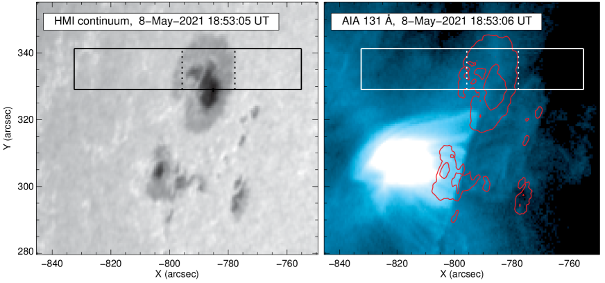
Figure 1: Left: HMI continuum showing AR 12822. The solid black rectangle marks the ViSP FOV. The inset dashed box shows the cropped FOV employed in Figure 3. Right: AIA 131 Å observations showing the solar flare in progress. As in the left panel, the white/dashed rectangles show the full/cropped ViSP FOV. Red contours mark the sunspot location, as seen in HMI continuum (left panel). The bright feature in the right panel shows the flare loops of a C-class flare peaking prior to the beginning of the ViSP observations.

The ViSP polarimetric scan ran from 18:52:39 to 19:31:19 UT 8 May 2021. It consists of 300 contiguous slit positions, separated by the slit width of 0.041″. It covers an angular extent of 12.3″ in the N-to-S direction. The field-of-view (FOV) covered by the lowest-magnification spectral arm of the ViSP (vcc1) is shown in Figure 1. The extent of the FOV along the slit, and the corresponding spatial sampling by the detector, are different for the three spectral arms: 75.9″ with 0.030″/px for camera vcc1 (Fe I), 62.3″ with 0.024″/px for camera vcc2 (Ca II H-line), and 49.4″  with 0.019″/px for camera vcc3 (Ca II 854 nm).

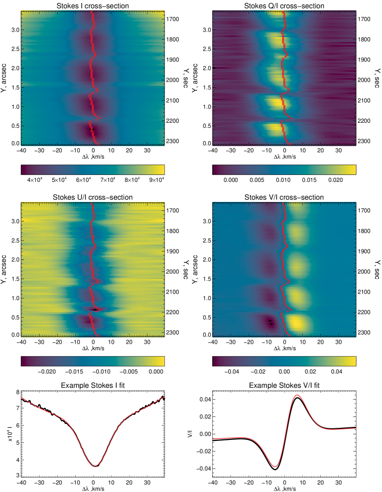
Figure 2: Full Ca II 854.2 nm spectral data of the fractional stokes parameters observed at the $X$ position and along the $Y$ range corresponding to the magenta dashed line in Figure 3. The red line tracks the center-of-gravity of Stokes $I$. The bottom panels show an example fit (red) to Stokes I and V/I data (black), for the spectra at Y=2150 sec in the top panels.

The dwell time for one slit position was 7.58 sec, consisting of 25 modulation cycles of 10 states each at a camera frame rate of 33 Hz. Because of the different intensity levels and instrument throughput values of the three spectral channels, the duty cycles of the three cameras were dramatically different, with the Fe I spectral window being integrated only 20% of the time with 6 ms exposures. The two Ca II spectral lines were observed with 66% duty cycle (20 ms exposures), to build sufficient signal-to-noise in the chromospheric Stokes $Q$, $U$, and $V$ signals. After integration, the slit was advanced by one full slit width (0.041″) for a new integration. Each of the 300 steps take 0.18 s, resulting in a time interval between slit positions of 7.76 s, for a total raster duration of 38.8 minutes. For the observations we analyze here, the ViSP FOV was rastered over 300 steps, with a total scan time of 38.8 min. This corresponds to an average slit speed projected onto the plane-of-the-sky (POS) of $v_{s}=3.83~{}\mathrm{km}/\mathrm{s}$.

The FOV covered by the ViSP scan is marked in Figure 1 relative to the Helioseismic and Magnetic Imager (HMI, Schou et al., 2012) white-light continuum and the Atmospheric Imaging Assembly (AIA, Lemen et al., 2012) extreme-ultraviolet 131 Å images. Shortly before the start of the ViSP data acquisition, a C8.6-class solar flare occurred to the SE of the active region. The location of the flare loops, which peaked in emission at 18:45 UT, are the bright feature in the right panel of Figure 1. The northern-most foot point of the flare loops intersects the penumbra of the larger sunspot observed by ViSP. Unfortunately, the short temporal duration and spatial coverage of the scan make it impossible to distinguish between flare-induced sunquakes and ubiquitous sub-photospheric umbral wave sources in AR 12822—e.g., Kosovichev & Sekii (2007), Besliu-Ionescu et al. (2017), Millar et al. (2021). A cursory examination of the HMI and AIA contemporaneous data also fails to identify any obvious oscillatory variations that can be unequivocally attributed to the flare.

For the analysis that follows, we restrict our attention to the cropped portion of the FOV that lies above the sunspot where strong magnetic fields and sensible polarization signal should be present. The two vertical dashed lines near $X=-795$ and $X=-775$ mark the E-W boundaries of this region-of-interest (ROI).

2.1 Data Reduction

Figure 2 displays a typical spectropolarimetric data cross-section obtained with the vcc3 camera. A robust oscillatory signal is present in all four Stokes parameters. The intensity profile consists of a narrow Gaussian core ($\Delta\lambda\approx 20$ km/s) and broad Lorentzian wings.

During the 8 May 2021 SV observations, a slight defocus of the ViSP collimator caused the appearance of considerable astigmatism for spectral configurations significantly away from Littrow. While vcc1 practically did not suffer any spectral defocus because of its proximity to the Littrow configuration ($3.31^{\circ}$), the spectral resolution of cameras vcc2 and vcc3 (respectively $7.52^{\circ}$ and $20.07^{\circ}$ from Littrow) was significantly impacted. Therefore, we did not attempt a full inversion of the Ca II 854 nm Stokes profiles. Instead, we simply applied a single Gaussian fit to the core and near wings of the intensity and $I\pm V$ profiles to estimate the line core intensity, central wavelength, line width, and Zeeman splitting. A representative Gaussian fit is presented in Figure 2. Assuming the line centers of Stokes $I$, $Q$ and $U$ occur close to the same wavelength position, the Gaussian fit also provides the position and value of the peak Stokes $Q$ and $U$ emissions. This assumption holds for the majority of the FOV, but has limitations discussed in section 2.2. From these linear polarization measurements, we calculate the linear polarization degree and azimuth,

$$P = \frac{\sqrt{Q^{2}+U^{2}}}{I}\;,$$ (1)

$$\Phi = \frac{1}{2}\arctan{\frac{U}{Q}}\;.$$ (2)

When the linear polarization is dominated by the Zeeman effect, the azimuth $\Phi$ also gives the direction of the magnetic field projected onto the POS (with a $180^{\circ}$ ambiguity). The circularly polarized Stokes $V$ signals yield the longitudinal magnetic field strength $B_{\rm LOS}\equiv B\cos\Theta$, where $\Theta$ is the angle between the magnetic field vector and the LOS. A simple application of the weak-field approximation (e.g., Landi Degl’Innocenti & Landolfi, 2004; Centeno, 2018) appears to be adequate to provide good profile fits down to the noise level of the polarized signal (about $0.2$% of Stokes $I$, in these observations), and was therefore used to estimate $B_{\rm LOS}$.

A proper description of the atmospheric dynamics at the time of the ViSP observations requires an adequate wavelength calibration of the spectral data. Because of the visibility of many telluric (i.e., Earth atmosphere’s) molecular lines in the Fe I 630 nm spectral range, this is rather easily achieved for the vcc1 data. In contrast, the lack of strong telluric lines in the Ca II 854 nm spectrum makes a precise wavelength calibration of the vcc3 data more difficult. The significant spectral smearing of these data due to the ViSP astigmatism further complicates the matter. In order to arrive at a meaningful estimation of the chromospheric dynamics in the ViSP data, we followed the following procedure:

1. We identified a small ($\sim 3$″$\times$4″) QS region to the E of the sunspot, where the photospheric dynamics is dominated by the granulation, resulting in highly symmetric distributions of positive and negative Doppler shift amplitudes for the lines of Fe I at 629.8 nm and 630.1 nm, with practically zero mean LOS velocity over the region. Referencing both lines to the O2 telluric line at 629.8 nm, we estimated a photospheric blue-shift of 1.65 km/s, consistent with the solar rotational velocity expected at the heliocentric coordinates of the observations;

2. We determined the center-of-gravity of the Fe I 853.8 nm line in the vcc3 data, and assumed it to be at rest with the photosphere probed by the Fe I lines in vcc1;

3. Finally, we referenced the center-of-gravity of the chromospheric Ca II 854.2 nm line to the photospheric reference of the Fe I 853.8 nm line.

The result of this wavelength calibration is that the zero-velocity reference of the Ca II 854.2 nm Doppler map in Fig. 3, averaged over the entire map, is red-shifted by about 1.53 km/s with respect to the QS photosphere.

Recent work by Felipe et al. (2021), suggests that magnetic field oscillations should not easily be detected with the Ca II 854 nm line. However, because of the sunspot’s location close to the limb, the $B_{\rm LOS}$ measurements derived from Stokes $V$ need not necessarily relate to changes in $|\bm{B}|$, but may well contain fluctuations in field orientation.

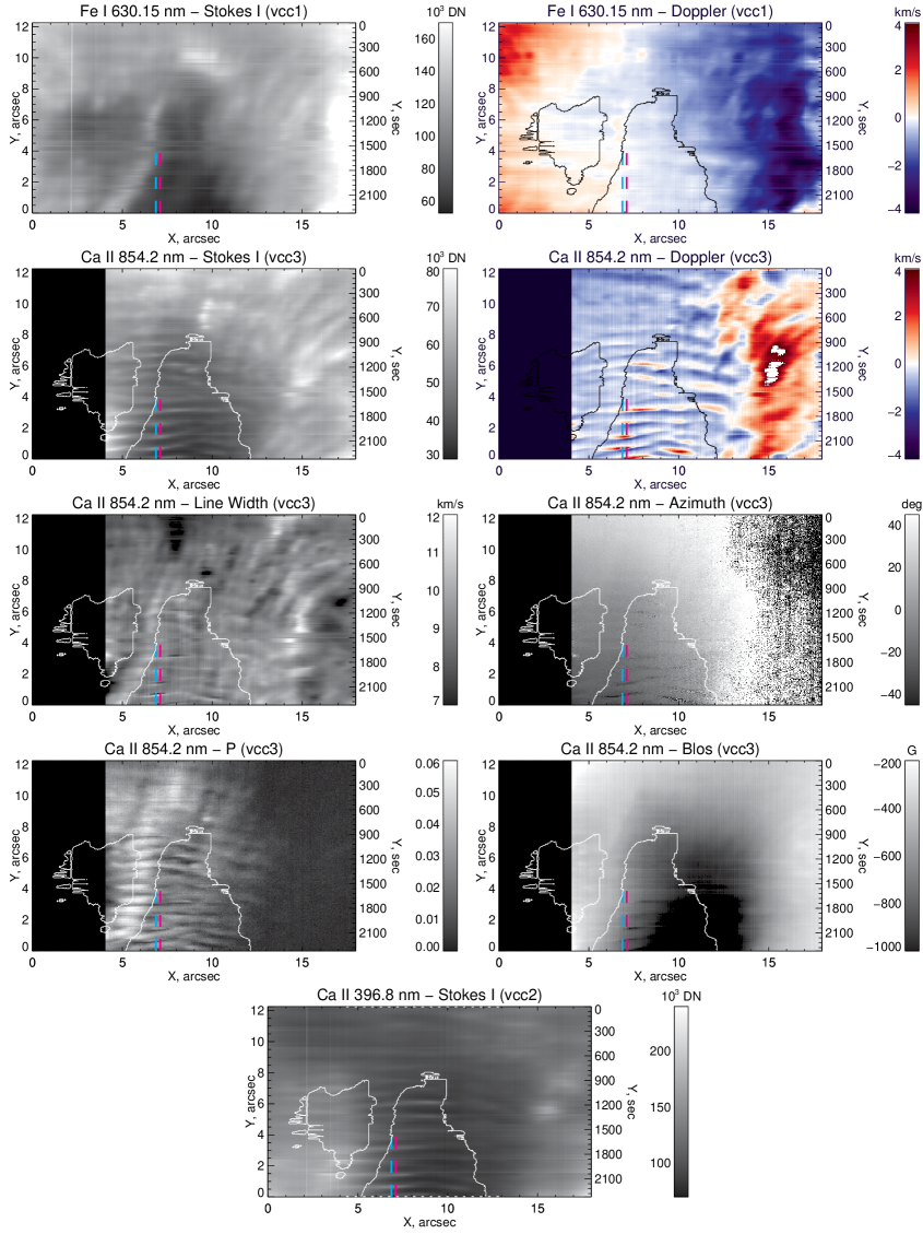
Figure 3: Active region scans from the ViSP SV campaign. The plots show a cropped subset of the full FOV, as shown in Figure 1. Each image is labeled with the spectral line and observed parameter. The cyan and magenta dashed lines shows the location of the umbral flash cross-sections examined in Figure 4. The solid white/black contour indicates the location of the sunspot umbra as determined from Fe I 630 nm intensity (top-left panel). We omit Ca II 854.2 data below 4″ due to artifacts of poor fits in this region.

Figure 3 shows data from the ViSP polarization scan over the sunspot ROI indicated in Figure 1. The top row displays intensity in the core of the photospheric Fe I 630 nm line and its LOS Doppler velocity. The second row provides the same for the chromospheric Ca II 854 nm line; derived magnetic parameters are presented in rows two to four. Finally, Ca II H 397 nm intensity is presented in the bottom panel.

The thin black/white contours indicate the approximate location of the umbra-penumbra boundary determined from the Fe I 630 nm line intensity. This is the boundary between the umbra and the penumbra at the photosphere. The Ca II resonance lines are expected to form 700 - 1400 km above this line. Owing to the large inclination of the LOS, the projection on the POS will shift the position of the Ca II signal directly above the Fe I signal some one-half to one arcsecond to the ENE. Wavelength-dependent atmospheric refraction will also shift the chromospheric and photospheric signals on the POS. A light bridge separates the E satellite umbra from the larger central umbra. Present in the E (left) umbra is the vertical ViSP hairline - used for calibration between the instrument cameras.

In Figure 3, the rastered ViSP data obtained at each value of $X$ are plotted in $Y$ against both slit position (left axis) and the time of the data acquisition (right axis). Convenient origins in time and N-S slit position have been selected to facilitate the analysis and display. We use both coordinates interchangeably in what follows to emphasize that the ViSP scan via a stepped slit necessarily mixes N-S spatial and temporal variations.

2.2 Summary of the Scans

The sunspot structure is readily apparent in the photospheric Fe I 630 nm intensity plot, showing the larger central and smaller E satellite (left) umbrae (also seen in HMI, Figure 1), separated by a thin light bridge. The surrounding penumbra is visible to the N and W (right) of these regions. There is no quiet sun in our ROI. The Doppler velocity scans exhibit the expected Evershed flow in the photosphere and the reverse chromospheric inflow from above (e.g., Teriaca et al., 2008).

Prominent in the Ca II scans are a series of nested ridges, running almost parallel to the horizontal E-W direction across the image. These ridges are striking in the Doppler velocity and $P$ scans. They are also present in line width, azimuth, $B_{\rm LOS}$, and intensity. We see these same ridges in the H-line intensity. The average N-S separation of these ridges in $Y$ is on the order of $0.5\arcsec$. A second more widely-separated set of horizontal ridges is also discernible in the Fe I scans. Their N-S spacing is slightly in excess of $1\arcsec$. Both sets of ridges are not strictly horizontal, but they are well-resolved over 300 pixels from N to S, and highly-structured—exhibiting both curvature and variation in brightness/thickness from E to W.

Observations of similar oscillatory ridge-like structures, sometimes referred to as ’herringbone’ patterns, were first observed in the photosphere by works including Thomas et al. (1984) and Lites et al. (1998), and later in the chromosphere with the Dunn Solar Telescope / Horizontal Grading Spectrograph by (Balasubramaniam et al., 2008).

The moving slit yields an image scan that may be neither purely temporal nor spatial, but could be a mixture of the two. It is not possible to determine from these observations alone whether the ridges originate from a large-scale coherent temporal pulsation of the entire umbra, or from the moving slit passing over a static spatial undulation, or from a sinusoidal disturbance progressing northward or southward across the sunspot. Previous observations of ’herringbone’ ridges are captured by sit-and-stare measurements, which produce images of x against t. Because ViSP’s moving slit creates images convolving spatial and temporal information in the vertical axis (creating an image of x against y and t), we lay out an argument in this section that the ridges observed by ViSP are not spatially-resolved structures, but are temporally-resolved, similar to the previous sit-and-stare observations.

Consider a progressive oscillatory disturbance moving northward across the POS at a speed $c$ with a spatial wavelength $\lambda_{c}$, and a temporal period $T_{c}$. The relative velocity between the average southward speed of the stepped moving slit and the progressive disturbance determines the resulting separation of ridges in $Y$. The relationship between the true (subscript “$c$”) and observed (no subscript) wavelengths and periods ($\lambda_{c}$, $\lambda$ and $T_{c}$, $T$ respectively), are

$$\frac{v_{s}+c}{c}=\frac{T_{c}}{T}=\frac{\lambda_{c}}{\lambda}\frac{v_{s}}{c},\$$ (3)

$$c=\frac{v_{s}}{T_{c}/T-1}=v_{s}\biggl{(}\frac{\lambda_{c}}{\lambda}-1\biggr{)}\;.$$ (4)

The observed period $T$ and wavelength $\lambda$ are related by $\lambda=Tv_{s}$, where $\lambda$ is the physical distance between ridges on the ViSP scans, and $T$ is the time between observations of the ridges. For oscillatory disturbances progressing southward, one simply replaces $c$ by $-c$ in these expressions.

Notice that in the extreme case of a coherent spatial pulsation of the entire sunspot ($\lambda_{c},c\to\infty$) the moving slit records the true period $T=T_{c}$. Likewise for a static spatial undulation ($T_{c}=\infty$), the moving slit returns the true wavelength $\lambda=\lambda_{c}$. Between these two extremes neither the recorded wavelength nor period will match their true POS values.

To distinguish spatial from temporal behavior we compare the ViSP observations with contextual (contemporaneous) observations of the photosphere/chromosphere obtained by HMI (intensity and Doppler measurements) and AIA (304 Å, 1600 Å and 1700 Å). These data have poorer spatial and temporal (per slit-position) resolution, however they have the advantages that they do not mix the spatial and temporal information and they extend (in both space and time) well beyond the ViSP scan. These data indicate fixed, spatially-coherent, patches of brightness oscillations in the sunspot umbra. This is entirely consistent with the usual behavior of chromospheric 3-minute umbral oscillations (Khomenko & Collados, 2015). Because the period of the AIA brightness oscillations match the period of the oscillations observed by ViSP, the ViSP ridges are not Doppler shifted by the moving slit. This reveals that the ridges do not arise from spatially-resolved waves traveling across the POS, but are instead purely temporal in character as the ViSP slit moves over the pulsating region.

Because of their spatially-coherent temporal and periodic nature, the ridges observed by ViSP cannot be a result of fine spatial structures within the umbra, such as intermixing hot and cool plasma elements (Socas-Navarro et al., 2000, 2009), filamentary structure (Socas-Navarro et al., 2009), two-component umbral structure (Centeno et al., 2005; de la Cruz Rodríguez et al., 2013), small-scale dynamic fibrils (Rouppe van der Voort & de la Cruz Rodríguez, 2013), cool jet-like structures (Yurchyshyn et al., 2014), etc.

In the penumbra to the NW of the umbra, the ridges are much broader and have a significant tilt relative to the $X$ and $Y$ directions. Here our slit is probably sampling some combination of temporal and spatial variability appropriate to running penumbral waves.

3 The Umbral Flash

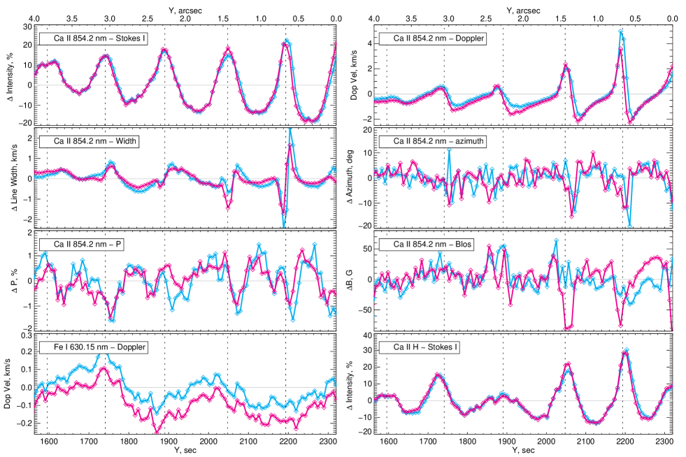
Figure 4: Detrended intensity, line width, azimuth, P and B LOS cross-sections, and raw Doppler cross-sections, along the cyan and magenta dashed lines in Figure 3. Vertical dashed lines show the approximate locations of the Ca II 854 nm intensity peaks.

Figure 4 provides a closer look at a portion of the chromospheric ridge structure. Here we plot a N-S cross-section through the Ca II parameters along the dashed cyan and magenta line segments plotted in Figure 3. The spectropolarimetric cross-section for the magenta line segment appear in Figure 2. The lower axis of Figure 4 uses the temporal $Y$ coordinate for the data acquisition and the upper axis uses the N-S spatial position of the slit at the time the data were obtained. With the exception of Doppler velocity, the parameters have all been detrended by a polynomial fit to suppress gradual variations across the ROI and to highlight the oscillatory signal. We also note that within this region, the line center of Stokes $Q$ differs from Stokes $I$ by about 3 km/s, as shown in Figure 2. Line centroids of Stokes $U$ and $V$ still follow $I$.

These data show a particularly revealing example of a chromospheric umbral flash, with the wave-train of shocks and rarefactions present in most of the Ca II parameters. For the chromospheric intensities, the extended shock compressions and intervening rarefaction cross-sections are broad, well-resolved, and symmetric about peaks and valleys. The dashed vertical lines in Figure 4 show the approximate locations of the shocks as identified by eye. The Ca II 854  nm Doppler and line-width time series differ significantly from the intensity profiles. Instead of symmetric rise and fall profiles, we see a steep rise and precipitous fall characteristic of a thin embedded subshock. Indeed the largest excursion near $Y=2200$ seconds occurs across just 4 $Y$-pixels/timesteps. The line width shows a somewhat broader zig-zag about the subshock.

In the magenta cross-section, the line-of-sight magnetic field (i.e., Stokes $V$) oscillates 180 degrees out of phase with the intensity parameters. The azimuth and linear polarization are also well-correlated with the subshock but have lower signal-to-noise ratios. There is a hint that they exhibit a negative spike at the greatest positive excursion of the Doppler width (equivalently, negative excursion of the Doppler velocity).

A careful examination of the contemporaneous AIA and HMI data indicates the umbral flash is confined to $Y$ values less than 3 to 4 arcseconds, and it has been oscillating there with a slowly varying temporal frequency throughout the duration of the ViSP data acquisition. The increase in the amplitude of the oscillation from left to right in Figure 4 is consistent with the slit moving southward into the stronger core of this stationary, steady, umbral flash. The temporal oscillation frequency present in Figure 4 is the same as that obtained from the AIA data during this epoch, meaning it has not been Doppler shifted by the moving ViSP slit (Equation 4). This is consistent with the umbral flash oscillating in place over a fixed spatial region near the center of the umbra. In other words, the motion of the slit does not shift the observed frequency from the true oscillation frequency. The spatial wavelength (bottom abscissa scale), however, is purely an artifact of the sit-stare-step method, and is given by $T_{c}/v_{s}$.

It is possible to estimate the parameters for these shocks. For example, let us consider the blue curve in the neighborhood of $Y=2200$. We find the peak POS pre-shock down-flow velocity at $Y=2190$ to be 5.22 km/s. The post-shock up-flow velocity is 1.70 km/s. Dividing by the cosine of the inclination angle (0.443) and assuming the motions are along a vertical magnetic flux tube near the center of the umbra we obtain a preshock downflow velocity of $u_{+}=$ 11.8 km/s and a postshock upflow velocity of $u_{-}=$ 3.83 km/s.

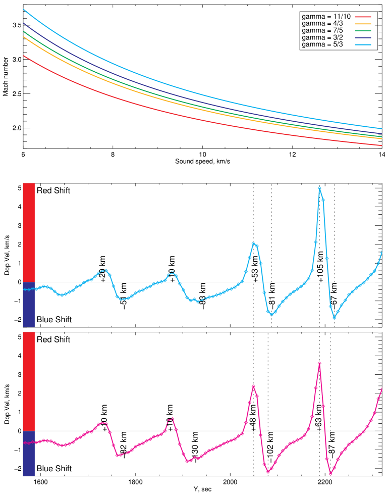
Figure 5: Top: Mach number of the largest shock in our observations (at Y$\approx 2200$ seconds in the cyan cross-section), for a reasonable range of sound speed and $\gamma$ values. Middle/Bottom: Cross-sections of Ca II 854.2 nm Doppler velocity along the cyan (middle) and magenta (bottom) cross-sections in Figure 3 Dashed lines indicate the shock locations. Following time, one sees a near-constant deceleration from blueshift to redshift behind the nonlinear pulses. As the shock forms, we see increased deceleration into red shift, followed by a rapid acceleration into blueshift, before repeating into the following shock.

Suppose the shock is moving upward along the vertical magnetic flux tube with a speed of $v$ km/s. In the rest frame of the shock, the ratio of the upstream to downstream velocities (and downstream to upstream densities) is given by the usual gas-dynamic Rankine-Hugoniot relations,

$${v+u_{+}\over v-u_{-}}={(\gamma+1)M^{2}\over 2+(\gamma-1)M^{2}}={\rho_{-}\over\rho_{+}}\;,$$ (5)

where $M=(v+u_{+})/c_{s}$ is the upstream Mach number, $c_{s}$ is the adiabatic sound speed, and $\gamma$ is the ratio of specific heats. Setting $v+u_{+}=c_{s}M$, and defining $\alpha$ as $\alpha=c_{s}/(u_{+}+u_{-})$, we obtain the following expression for the Mach number:

$$M={(\gamma+1)\over 4\alpha}+\sqrt{1+{(\gamma+1)^{2}\over 16\alpha^{2}}}\;.$$ (6)

Once $M$ is obtained, the shock velocity $v$ is readily computed, as well as the ratio of the downstream to upstream gas pressure

$${p_{-}\over p_{+}}={2\gamma M^{2}-(\gamma-1)\over\gamma+1}\;,$$ (7)

and the analogous temperature ratio.

The ViSP observations give $u_{+}+u_{-}=$ 15.6 km/s for the strongest blue shock shown in Figure 4. Taking, for example, $\gamma=1.1$ to account for Hydrogen ionization, and $c=10~{}\mathrm{km}\,\mathrm{s}^{-1}$, one obtains: $M=2.11$, $v=9.3$ km/s, $\rho_{-}/\rho_{+}=3.82$, $p_{-}/p_{+}=4.62$, and $T_{-}/T_{+}=1.21$. Larger sound speeds produce weaker shocks which propagate faster; larger ratios of specific heats produce stronger shocks which also propagate faster. The top panel of Figure 5 displays the Mach number (ordinate) for this strongest observed blue shock ($u_{+}+u_{-}=$ 15.6 km/s) for a range of upstream sound speeds ($c$, abscissa) and several adiabatic indices (colored curves). We note that these parameters are estimates, given that the Rankine-Hugoniot relation assumes an idealized infinite planar shock propagating along a constant uniform magnetic field. The fact we see a molderate decrease in magnetic field strength behind the shock does not invalidate these estimates.

The Stokes $V$ and linear polarization $P$ signals are broadly consistent with a modest expansion of the cross-sectional area of the magnetic flux tube (decrease in magnetic field strength) expected from the gas pressure increase behind the shock. The nominal magnetic field strength is of order 500-600 G, so $\Delta B/B\approx 0.1$. As would be expected from such an interpretation, the magnetic fluctuations are detected only for the strongest shocks.

The variation in the line-width zig-zag across the shock is interesting and robust. It too is most pronounced for the strong shocks, and is largely absent in the nonlinear pulses. We are presently unable to identify a compelling physical explanation for it. The dramatic change in slope of the Doppler velocity in passing from blue-shifted (negative values) to red-shifted (positive values) suggests a quasi-free-fall rarefaction front may lie in between shocks. The attendant rapid expansion of the material could lead to cooling and might also tend to stretch out, or elongate turbulent motions set up in the post-shock flow. Both of these effects could contribute to a reduced line width. Likewise the enhancement of the line-width downstream of the shock could arise from a combination of compressive heating and post-shock turbulence. On the other hand, one must acknowledge that the line source function may encompass non-equilibrium and dynamical complications, including, for example, analogous K2V and K2R emission processes observed in the K-line. A definitive explanation of this line width zig-zag will require a careful spectral synthesis.

The lack of asymmetry in Stokes $I$ indicates the radiative transfer in the line core is optically-thick around the shock compression. The ratio of the maximum to minimum values of Stokes $I$ is close to 3/2—the fourth root of this number is 1.10, which is comparable to, but comfortably below our estimate of $T_{-}/T_{+}$ of 1.21 given above.

One can compute the integral under the undetrended Doppler velocity to determine if there is a net flow of material along the magnetic flux tube over one cycle of oscillation. The areas (expressed in km) between the zero-crossings of the blue and magenta curve POS Doppler velocities are provided in the bottom panels of Figure 5. We have not divided by the cosine of the inclination angle to the LOS (0.443). Taking into account this factor of 2.25 one observes that the range of upward and downward displacements per oscillation cycle are no more than a density scale height. For the weaker nonlinear pulses there is a net upward motion of the material per cycle. However, for the strongest shock the net motion is downward. The former behavior is consistent with the general notion that nonlinear waves contribute an upward-directed pressure gradient and tend to elevate material in a flux tube relative to its neutral hydrostatic altitude. In the latter case, where strong localized shocks are present, the precipitous quasi-free-fall redshift of the material in front of the shock may carry the material farther than the subsequent upflow behind the shock. Indeed, it is tempting to speculate that the over time, the nonlinear pulses eventually raise too much plasma above its neutral level and the subsequent formation of strong shocks in the quasi-free-fall downflow is how the mature umbral flash addresses this untenable situation.

The complex projection and atmospheric refractive POS offsets between the chromospheric and photospheric oscillations make it difficult to investigate any potential photospheric roots of the umbral flash. Never-the-less the Fe I Doppler velocity appears to attain its maximal blue shifts and red shifts close to the time of passage of the chromospheric shocks. Equivalently, the underlying photospheric oscillation has a period close to 5 minutes, or nearly twice that of the 150 second separation of shocks in the chromosphere. This is reminiscent of the period/frequency doubling often seen in highly nonlinear systems.

4 Conclusion

In this paper we examined DKIST/ViSP Science Verification (SV) observations to assess high-spatial and temporal spectropolarimetric observations of chromospheric and photospheric oscillations in a sunspot. We detected the ubiquitous running penumbral waves, chromospheric 3-min oscillations, and an umbral flash, with the detected periods affected by the motion of the moving ViSP slit. All of these phenomena have been observed and studied for decades. However, included in these oscillations data are the Stokes $V$ and linear polarization ($P=\sqrt{U^{2}+Q^{2}}/I$) of the chromospheric Ca II 854.2 nm line, which provide rich spectropolarimetric signatures of the umbral flash.

Owing to residual spectrograph astigmatism at the time of the SV campaign, the data did not achieve sufficient spectral resolution to justify a detailed Stokes inversion of Ca II 854 nm. Despite these drawbacks, the SV observations provide tantalizing hints of previously unknown spatial, temporal and spectral behaviors associated with dynamical processes associated with a sunspot umbra. In particular, we find polarimetric evidence of a wave-train of shocks and rarefactions over time scales of 0.16 seconds, the likes of which, to the authors’ best knowledge, have not been detected before. Across the shock train, we find values of $M=1.88$, $v=10.6~{}\mathrm{km}\,\mathrm{s}^{-1}$, $\rho_{-}/\rho_{+}=3.15$, $p_{-}/p_{+}=3.66$, and $T_{-}/T_{+}=1.16$. These parameters are consist with the ranges of shock parameters calculated in other work, e.g. Anan et al. (2019b).

As ViSP has begun science commissioning and normal operations in 2022, new observations will further push the spatial and spectral limitations of the data reported here, providing further clarity to the dynamic oscillations found within the chromosphere and photosphere.

References

- Anan et al. (2019a) Anan, T., Schad, T. A., Jaeggli, S. A., & Tarr, L. A. 2019a, ApJ, 882, 161, doi: 10.3847/1538-4357/ab357f
- Anan et al. (2019b) —. 2019b, ApJ, 882, 161, doi: 10.3847/1538-4357/ab357f
- Balasubramaniam et al. (2008) Balasubramaniam, K. S., Pevtsov, A. A., & Olmschenk, S. 2008, in Astronomical Society of the Pacific Conference Series, Vol. 383, Subsurface and Atmospheric Influences on Solar Activity, ed. R. Howe, R. W. Komm, K. S. Balasubramaniam, & G. J. D. Petrie, 279
- Bard & Carlsson (2010) Bard, S., & Carlsson, M. 2010, ApJ, 722, 888, doi: 10.1088/0004-637X/722/1/888
- Beckers & Tallant (1969) Beckers, J. M., & Tallant, P. E. 1969, Sol. Phys., 7, 351, doi: 10.1007/BF00146140
- Besliu-Ionescu et al. (2017) Besliu-Ionescu, D., Donea, A., & Cally, P. 2017, Sun and Geosphere, 12, 59
- Bose et al. (2019) Bose, S., Henriques, V. M. J., Rouppe van der Voort, L., & Pereira, T. M. D. 2019, A&A, 627, A46, doi: 10.1051/0004-6361/201935289
- Centeno (2018) Centeno, R. 2018, ApJ, 866, 89, doi: 10.3847/1538-4357/aae087
- Centeno et al. (2006) Centeno, R., Collados, M., & Trujillo Bueno, J. 2006, ApJ, 640, 1153, doi: 10.1086/500185
- Centeno et al. (2009) —. 2009, ApJ, 692, 1211, doi: 10.1088/0004-637X/692/2/1211
- Centeno et al. (2005) Centeno, R., Socas-Navarro, H., Collados, M., & Trujillo Bueno, J. 2005, ApJ, 635, 670, doi: 10.1086/497393
- de la Cruz Rodríguez et al. (2013) de la Cruz Rodríguez, J., Rouppe van der Voort, L., Socas-Navarro, H., & van Noort, M. 2013, A&A, 556, A115, doi: 10.1051/0004-6361/201321629
- De Wijn et al. (2022) De Wijn, A. G., Casini, R., Carlile, A., & etal. 2022, Solar Physics, 297, 22
- Felipe et al. (2014) Felipe, T., Socas-Navarro, H., & Khomenko, E. 2014, ApJ, 795, 9, doi: 10.1088/0004-637X/795/1/9
- Felipe et al. (2018) Felipe, T., Socas-Navarro, H., & Przybylski, D. 2018, A&A, 614, A73, doi: 10.1051/0004-6361/201732169
- Felipe et al. (2021) Felipe, T., Socas Navarro, H., Sangeetha, C. R., & Milic, I. 2021, ApJ, 918, 47, doi: 10.3847/1538-4357/ac111c
- Henriques et al. (2020) Henriques, V. M. J., Nelson, C. J., Rouppe van der Voort, L. H. M., & Mathioudakis, M. 2020, A&A, 642, A215, doi: 10.1051/0004-6361/202038538
- Houston et al. (2018) Houston, S. J., Jess, D. B., Asensio Ramos, A., et al. 2018, ApJ, 860, 28, doi: 10.3847/1538-4357/aab366
- Houston et al. (2020) Houston, S. J., Jess, D. B., Keppens, R., et al. 2020, ApJ, 892, 49, doi: 10.3847/1538-4357/ab7a90
- Joshi & de la Cruz Rodríguez (2018) Joshi, J., & de la Cruz Rodríguez, J. 2018, A&A, 619, A63, doi: 10.1051/0004-6361/201832955
- Khomenko & Collados (2015) Khomenko, E., & Collados, M. 2015, Living Reviews in Solar Physics, 12, 6
- Kosovichev & Sekii (2007) Kosovichev, A. G., & Sekii, T. 2007, ApJ, 670, L147, doi: 10.1086/524298
- Kuźma et al. (2017a) Kuźma, B., Murawski, K., Kayshap, P., et al. 2017a, ApJ, 849, 78, doi: 10.3847/1538-4357/aa8ea1
- Kuźma et al. (2017b) Kuźma, B., Murawski, K., Zaqarashvili, T. V., Konkol, P., & Mignone, A. 2017b, A&A, 597, A133, doi: 10.1051/0004-6361/201628747
- Landi Degl’Innocenti & Landolfi (2004) Landi Degl’Innocenti, E., & Landolfi, M. 2004, Polarization in Spectral Lines, Vol. 307, doi: 10.1007/978-1-4020-2415-3
- Lemen et al. (2012) Lemen, J. R., Title, A. M., Akin, D. J., et al. 2012, Sol. Phys., 275, 17, doi: 10.1007/s11207-011-9776-8
- Lites (1992) Lites, B. W. 1992, in NATO Advanced Study Institute (ASI) Series C, Vol. 375, Sunspots. Theory and Observations, ed. J. H. Thomas & N. O. Weiss, 261
- Lites et al. (1998) Lites, B. W., Thomas, J. H., Bogdan, T. J., & Cally, P. S. 1998, ApJ, 497, 464, doi: 10.1086/305451
- Löhner-Böttcher (2016) Löhner-Böttcher, J. 2016, PhD thesis, Albert Ludwigs University of Freiburg, Germany
- Madsen et al. (2015) Madsen, C. A., Tian, H., & DeLuca, E. E. 2015, ApJ, 800, 129, doi: 10.1088/0004-637X/800/2/129
- Millar et al. (2021) Millar, D. C. L., Fletcher, L., & Milligan, R. O. 2021, MNRAS, 503, 2444, doi: 10.1093/mnras/stab642
- Molnar et al. (2021) Molnar, M. E., Reardon, K. P., Cranmer, S. R., et al. 2021, ApJ, 920, 125, doi: 10.3847/1538-4357/ac1515
- Pietarila et al. (2007) Pietarila, A., Socas-Navarro, H., & Bogdan, T. 2007, ApJ, 663, 1386, doi: 10.1086/518714
- Pietarila et al. (2006) Pietarila, A., Socas-Navarro, H., Bogdan, T., Carlsson, M., & Stein, R. F. 2006, ApJ, 640, 1142, doi: 10.1086/500240
- Rimmele et al. (2020) Rimmele, T. R., Warner, M., Keil, S. L., et al. 2020, Sol. Phys., 295, 172, doi: 10.1007/s11207-020-01736-7
- Rouppe van der Voort & de la Cruz Rodríguez (2013) Rouppe van der Voort, L., & de la Cruz Rodríguez, J. 2013, ApJ, 776, 56, doi: 10.1088/0004-637X/776/1/56
- Sadykov et al. (2021) Sadykov, V. M., Kitiashvili, I. N., Kosovichev, A. G., & Wray, A. A. 2021, ApJ, 909, 35, doi: 10.3847/1538-4357/abd9c7
- Schou et al. (2012) Schou, J., Scherrer, P. H., Bush, R. I., et al. 2012, Sol. Phys., 275, 229, doi: 10.1007/s11207-011-9842-2
- Schultz & White (1974) Schultz, R. B., & White, O. R. 1974, Sol. Phys., 35, 309, doi: 10.1007/BF00151951
- Snow & Hillier (2021) Snow, B., & Hillier, A. 2021, MNRAS, 506, 1334, doi: 10.1093/mnras/stab1672
- Socas-Navarro et al. (2009) Socas-Navarro, H., McIntosh, S. W., Centeno, R., de Wijn, A. G., & Lites, B. W. 2009, ApJ, 696, 1683, doi: 10.1088/0004-637X/696/2/1683
- Socas-Navarro et al. (2000) Socas-Navarro, H., Trujillo Bueno, J., & Ruiz Cobo, B. 2000, Science, 288, 1396, doi: 10.1126/science.288.5470.1396
- Song et al. (2017) Song, D., Chae, J., Yurchyshyn, V., et al. 2017, ApJ, 835, 240, doi: 10.3847/1538-4357/835/2/240
- Stangalini et al. (2018) Stangalini, M., Jafarzadeh, S., Ermolli, I., et al. 2018, ApJ, 869, 110, doi: 10.3847/1538-4357/aaec7b
- Stangalini et al. (2021a) Stangalini, M., Baker, D., Valori, G., et al. 2021a, Philosophical Transactions of the Royal Society of London Series A, 379, 20200216, doi: 10.1098/rsta.2020.0216
- Stangalini et al. (2021b) Stangalini, M., Jess, D. B., Verth, G., et al. 2021b, A&A, 649, A169, doi: 10.1051/0004-6361/202140429
- Teriaca et al. (2008) Teriaca, L., Curdt, W., & Solanki, S. K. 2008, A&A, 491, L5, doi: 10.1051/0004-6361:200810209
- Thomas et al. (1984) Thomas, J. H., Cram, L. E., & Nye, A. H. 1984, ApJ, 285, 368, doi: 10.1086/162514
- Thomas & Weiss (2012) Thomas, J. H., & Weiss, N. O. 2012, Sunspots and Starspots (Cambridge, UK: Cambridge Univ. Press), doi: 10.1017/CBO9780511536342
- Weiss & Proctor (2014) Weiss, N. O., & Proctor, M. R. E. 2014, Magnetoconvection (Cambridge, UK: Cambridge Univ. Press), doi: 10.1017/CBO9780511667459
- Yurchyshyn et al. (2014) Yurchyshyn, V., Abramenko, V., Kosovichev, A., & Goode, P. 2014, ApJ, 787, 58, doi: 10.1088/0004-637X/787/1/58
- Yurchyshyn et al. (2020) Yurchyshyn, V., Kilcik, A., Şahin, S., Abramenko, V., & Lim, E.-K. 2020, ApJ, 896, 150, doi: 10.3847/1538-4357/ab91b8