Simple and efficient four-cycle counting on sparse graphs

Abstract

We consider the problem of counting 4-cycles ($C_{4}$) in an undirected graph $G$ of $n$ vertices and $m$ edges (in bipartite graphs, 4-cycles are also often referred to as butterflies). There have been a number of previous algorithms for this problem based on sorting the graph by degree and using randomized hash tables. These are appealing in theory due to compact storage and fast access on average. But, the performance of hash tables can degrade unpredictably and are also vulnerable to adversarial input.

We develop a new simpler algorithm for counting $C_{4}$ requiring $O(m\bar{\delta}(G))$ time and $O(n)$ space, where $\bar{\delta}(G)\leq O(\sqrt{m})$ is the average degeneracy parameter introduced by Burkhardt, Faber & Harris (2020). It has several practical improvements over previous algorithms; for example, it is fully deterministic, does not require any sorting of the input graph, and uses only addition and array access in its inner loops. To the best of our knowledge, all previous efficient algorithms for $C_{4}$ counting have required $\Omega(m)$ space in addition to storing the input graph.

Our algorithm is very simple and easily adapted to count 4-cycles incident to each vertex and edge. Empirical tests demonstrate that our array-based approach is $4\times$ – $7\times$ faster on average compared to popular hash table implementations.

Keywords: graph, 4-cycle, four-cycle, counting, butterfly

1 Introduction

Let $G=(V,E)$ be an undirected graph, with $n=|V|$ vertices and $m=|E|$ edges. A $k$-cycle in $G$, denoted $C_{k}$, is a sequence of $k$ distinct adjacent edges that begins and ends with the same vertex without repeating vertices. Cycles are fundamental building blocks to larger graph structures and often denote important properties. The $C_{3}$ (i.e. triangle) in particular has been well-studied for its role in connectivity, clustering, and centrality [30, 13, 16, 10]. Today there is interest in analyzing fundamental 4-node subgraph patterns in large, sparse graphs.

The runtime of graph algorithms is often measured in terms of $m$ and $n$. For example, a straightforward triangle-counting algorithm may run in $O(m^{3/2})$ time. Such super-linear runtimes are impractical on large-scale, sparse graphs. More carefully designed algorithms take greater advantage of the graph structure and thereby require a finer measure of the runtime, often in terms of “sparsity” parameters. One such parameter is the core number $\kappa(G)$, which is the largest minimum degree of any subgraph. This is closely related to the arboricity $a(G)$, which is the minimum number of forests into which the edges can be partitioned. This allows for a tighter analysis of the performance. An alternative measure related to the arboricity is a new parameter called the average degeneracy, introduced in 2020 by Burkhardt, Faber & Harris [11]. It is particularly powerful and defined as

$$\bar{\delta}(G)=\frac{1}{m}\sum_{uv\in E}\min\{d(u),d(v)\},$$

where $d(x)$ is the degree of any vertex $x$. It is known that $\bar{\delta}(G)\leq 2a(G)$ and $a(G)\leq\kappa(G)<2a(G)\leq O(\sqrt{m})$, and $\bar{\delta}(G)$ can be much smaller than $a(G)$ or $\kappa(G)$. In our experiments on real-world graphs we have found that on average $\bar{\delta}(G)$ is about $3\times$ smaller than $\kappa(G)$, and on some graphs it was $6\times$ smaller.

There has been interest in counting 4-cycles in bipartite graphs as these can suggest similarity or closeness between vertices [27, 28, 32, 29]. In this context, a $C_{4}$ is often called a butterfly. For example, a $C_{4}$ in a user-item bipartite graph represents groups of users that select the same subset of items, and may therefore have similar interests. Recently, Wang et al. [28, 29] developed an algorithm with $O(m\bar{\delta}(G))$ expected runtime and $O(m)$ space based on sorting vertices. Their algorithm and many of the other previous algorithms have used hash tables freely; as a result, they are actually randomized algorithms.

The algorithm of [28, 29] was designed for bipartite graphs, but it works for general sparse graphs. This is the current state of the art for efficient $C_{4}$ counting. Although this algorithm is relatively straightforward on its own, it suffers from a few shortcomings which can make it less practical for large-scale computations. As we have mentioned, it uses randomized hash tables. It also requires computing binomial coefficients in its inner loop, which may be slow. There are a number of optimizations which can reduce these costs; for example, [29] suggests using a bin-sort pass to re-order the input graph by vertex degree. Adding in these optimizations can then make the implementation significantly more complex.

In this paper, we develop algorithms for $C_{4}$-counting that are simple, direct, and efficient. Our main improvements to the state-of-the-art are: (i) asymptotically less space (ii) deterministic runtime (iii) avoidance of binomial coefficients. Moreover, our experiments show that using an array is $4\times$ – $7\times$ faster than using popular hash tables. We summarize our results as follows.

Theorem 1.

Counting 4-cycles in $G$ takes $O(m\bar{\delta}(G))$ time and $O(n)$ space.

Theorem 2.

Counting 4-cycles incident to each vertex in $G$ takes $O(m\bar{\delta}(G))$ time and $O(n)$ space.

Theorem 3.

Counting 4-cycles incident to each edge in $G$ takes $O(m\bar{\delta}(G))$ time and $O(m+n)$ space.

Theorem 4.

Enumerating 4-cycles in $G$ takes $O(m\bar{\delta}(G)+\#C_{4})$ time and $O(n)$ space.

We emphasize that $G$ can be provided with an arbitrary ordering of the neighbors of each vertex. These asymptotic bounds are similar to the previous algorithms but there are two main differences. First, they are completely deterministic; in particular, the algorithms avoid the use of hash tables. Second, the space complexity is just linear in the vertex count (ignoring the cost of storing the input graph). To the best of our knowledge, all previous efficient algorithms for $C_{4}$ counting have required $\Omega(m)$ additional space.

These differences may seem minor but have important practical consequences. Let us summarize some other key reasons these differences can be significant.

Determinism vs. randomness:

The hash table is a powerful, versatile data structure which is ubiquitous in algorithm design. It has essentially optimal memory usage, linear in the size of its data, as well as constant-time access on average. However, in addition to theoretical issues about the role of randomness, it has its downsides in practice. First, it is relatively costly to implement, requiring a good hash function and code to handle collisions. Hash tables using chaining are not cache friendly, and those based on probing require careful maintenance of the load factor. Many programming languages provide hash table implementations for convenience but are of varying quality. We discuss this issue further in Section 5, where we demonstrate empirically that hash tables may be an order of magnitude slower than direct table access.

In addition, like all randomized algorithms, hash table operations can have unpredictable or unreproducible behavior. More seriously, it can open the door to catastrophically bad performance on adversarial inputs [14]. This can be partially mitigated by using stronger hash functions, e.g. [7]. By using a deterministic algorithm with worst-case guarantees, we eliminate all such issues at a stroke.

Cost of graph storage:

In some applications, we may wish to run our algorithm on very large inputs using a single machine [25, 24, 23, 19, 20]. Here, the graph may require hundreds of gigabytes to store, and we can afford to keep at most one copy in memory at a time. (By contrast, the number of vertices is typically more modest, requiring only megabytes of storage.) Any storage overhead of $\omega(m)$ is out of the question. Storage overheads of $\Omega(m)$ are painful and best avoided as much as possible. Note that many previous $C_{4}$-counting algorithms may have hidden $\Omega(m)$ costs for scratch-space to sort the input graph by vertex degree.

Read-only graph access:

Furthermore, because of the large size of the input graph, it is often desired to use “graph packages,” which are responsible for maintaining and updating the graph and communicating it across a network; for example, see [15]. It may be running multiple graph algorithms simultaneously (e.g. 4-cycle counting, $k$-core extraction, 3-cycle counting). In these cases, the individual graph algorithms should not modify the graph storage itself.

There is one other algorithmic improvement worth mentioning. In our algorithms, we do not explicitly compute binomial coefficients. Instead, we update the counts in a specific order leading to a direct sum equating to the binomial coefficient. In our experiments we found this slightly improved the running time. This also eliminates numerical complications from multiplication, which could potentially overflow or lose precision. Notably, this technique would also simplify and improve the current hash-based methods [27, 28, 32, 29] by eliminating the second pass over the graph.

We have found that other $C_{4}$-counting algorithms presented in prior works such as [28, 29], although conceptually simple, are broken up into multiple sub-algorithms with unclear data structures and control flow. This can make it hard for users to implement. We have tried to present our algorithm in a single listing, with only basic and explicit data structures.

1.1 Related algorithms

When considering 4-cycles, one must be careful to distinguish between algorithms that detect 4-cycles, count 4-cycles, and enumerate 4-cycles. A classical combinatorial result [8] is that graphs with many edges are guaranteed to contain many 4-cycles. Hence, 4-cycle detection is an inherently simpler problem and algorithms for it can focus only on highly sparse graphs. For instance, there is a combinatorial algorithm of [4] to detect $C_{4}$ in $O(m^{4/3})$ time. Note that this is completely different from the situation for 3-cycles, where there exist triangle-free graphs with $\Theta(n^{2})$ edges.

For the problem of enumerating 4-cycles, the runtime typically should be linear in $\#C_{4}$ (the number of copies of $C_{4}$ in the graph). Again, such algorithms can focus on sparse graphs, as otherwise $\#C_{4}$ is guaranteed to be large. Recently, Abboud et al. [2] proposed an algorithm to enumerate 4-cycles with runtime $\tilde{O}(\min\{n^{2},m^{4/3}\}+\#C_{4})$ time and $\tilde{O}(\min\{n^{2},m^{4/3}\})$ space (where $\tilde{O}(\cdot)$ hides logarithmic terms). The algorithm of [29] can also enumerate 4-cycles with $O(m\bar{\delta}(G)+\#C_{4})\leq O(m^{3/2}+\#C_{4})$ time and $O(m)$ space. There is also evidence that runtime $\Omega(\min\{n^{2},m^{4/3}\}+\#C_{4})$ is necessary for 4-cycle enumeration [18, 1].

For the harder problem of 4-cycle counting, there are two main approaches. The first of which are algorithms based on fast matrix multiplication [4, 5, 6]. The best result in general for 4-cycle counting takes $n^{\omega+o(1)}$ time [6], where $\omega$ is the matrix power exponent. For sparse graphs, Williams et al. described a randomized algorithm with $m^{\frac{4\omega-1}{2\omega+1}+o(1)}$ runtime [31], which is $O(m^{1.48})$ given current bounds $\omega\leq 2.37286$ [3]. We emphasize that such algorithms are not practical for three distinct reasons: (i) For large sparse graphs, we desire runtimes that are nearly linear in $m$, which may depend on graph sparsity parameters such as $\bar{\delta}$; (ii) fast matrix multiplications inherently requires super-linear storage to carry out recursive matrix subdivisions; (iii) fast matrix multiplications, with the possible exception of Strassen’s algorithm, have very high constant factors and are generally considered impractical.

A second approach is to use combinatorial algorithms to count 4-cycles. This is the approach we adopt. These algorithms can take advantage of various types of graph sparsity; in addition, since they are based on simple practical data structures, the hidden constants are small and reasonable. For example, the algorithm of [27] runs in $O\left(\min\{\sum_{u\in L}d(u)^{2},\sum_{v\in R}d(v)^{2}\}\right)$ time and $O(n)$ space for a bipartite graph $G=(L\cup R,E)$. See also [17, 26] for similar algorithms.

We also note that there are many related algorithms for the simpler task of counting a 3-cycle (i.e. triangle). Note that, in contrast to the situation with four-cyles, there exist triangle-free graphs with $\Theta(m^{2})$ edges; for this reason, triangle-counting, triangle-enumeration, and triangle-detection tend to have similar algorithmic behavior. In particular, a sparse graph can have $\Theta(m^{3/2})$ triangles, and so an optimal triangle-enumeration algorithm should take $O(m^{3/2})$ time. Tighter bounds were given in 1985 by Chiba and Nishizeki [12] using arboricity $a(G)$; they gave an efficient, deterministic algorithm to enumerate triangles in $G$ with $O(ma(G))$ runtime They also provided a deterministic algorithm to count 4-cycles with $O(ma(G))$ runtime and $O(m)$ space. There are also algorithms based on fast matrix multiplication to count 3-cycles in $m^{\frac{2\omega}{\omega+1}+o(1)}\leq O(m^{1.41})$ time.

1.2 Notation

The vertices of the graph are assumed to have labels in $[n]=\{1,\dots,n\}$. We use $uv$ as shorthand for an edge $\{u,v\}$ when convenient. The neighborhood of a vertex $v$ is given by $N(v)=\{u:uv\in E\}$ and $d(v)=\lvert N(v)\rvert$ is its degree. We define a total order of $V$ by setting $u\prec v$ if $d(u)<d(v)$; if $d(u)=d(v)$, we break ties arbitrarily (e.g. by vertex ID).

A simple cycle of length $k$ is denoted by $C_{k}$. Note that any 4-cycle $x,y,z,w$ has eight related 4-cycles, which can be obtained by shifting the sequence (e.g. $y,z,w,x$), or by reversing the sequence (e.g. $x,w,z,y$). In counting distinct 4-cycles, we would count all eight such cycles as just a single $C_{4}$. We use $\lozenge(G)$ for the total number of distinct 4-cycles in $G$ and likewise $\lozenge(v)$ and $\lozenge(e)$, respectively, for the number of distinct 4-cycles involving a vertex $v$ and an edge $e$.

2 Principal algorithm

Our principal solution for counting all 4-cycles is given in Algorithm 1. We emphasize that the algorithm does not require explicit ordering of vertices in the graph data structure. We can determine $u\prec v$ during the runtime in constant-time (by looking up the degrees of $u$ and $v$). In Section 4 we describe how this algorithm can be optimized if the data structure were allowed to be pre-sorted by degree order, which eliminates many conditional checks.

Algorithm 1 4-cycle counting

1:zero-initialized array $L$ of size $n$ indexed by $V$

2:for $v\in V$ do

3:     for $u\in N(v)$ do

4:         if $u\prec v$ then

5:              for $y\in N(u)$ do

6:                  if $y\prec v$ then

7:                       set $\lozenge(G)\coloneqq\lozenge(G)+L(y)$

8:                       set $L(y)\coloneqq L(y)+1$                                                

9:     for $u\in N(v)$ do

10:         if $u\prec v$ then

11:              for $y\in N(u)$ do

12:                  set $L(y)\coloneqq 0$                             

To ensure that each $C_{4}$ is counted exactly once, we require $v$ to have higher degree (or label in the case of tie) than $u,w$, and $y$. The array $L$ is used to count the number of vertices $u\in N(v)$ where $u\prec v$ and $u$ itself has a neighbor $y\prec v$. There are $\binom{L(y)}{2}$ unique combinations of neighbor pairs $u,u^{\prime}$ that give a $C_{4}$ of the form $\{v,u,y,u^{\prime}\}$. To avoid spurious counting from subsequent starting vertices, the second pass at Lines 9 – 12 clears the $L$ table. These steps are repeated for every vertex in $G$.

Note that Algorithm 1 does not explicitly compute the binomial coefficient; instead it is implicitly computed via the identity $\sum_{i}^{L(y)-1}i=\binom{L(y)}{2}$. This observation can be used to obtain a particularly elegant variant of Algorithm 1 using hash tables in place of the $L$ array, which eliminates the second pass (Lines 9 – 12). See Appendix A for further details.

Before the formal analysis, let us consider a few simple cases for illustration. Consider a $C_{4}$ as shown in Figure 1, where we suppose that $1\prec 2\prec 3\prec 4$.

Figure 1: A simple cycle of length 4 ($C_{4}$).

We begin in order from vertex $1$ in sequence to vertex $4$. Vertex $1$ is skipped because its neighbors do not precede it in degree or label. From vertex $2$ we get its neighbor $1$ but no updates can be made to $L$ because $4$ does not precede $2$. At vertex $3$ only the $L(1)$ value can be incremented, due to vertex $2$, but since the update to $L(1)$ is after the update to $\lozenge(G)$, then no 4-cycle can be detected. The $L(1)$ value is reset to zero before proceeding to vertex $4$ to avoid spurious counting. Finally, from $4$ we find $L(2)$ is incremented by $1$ and $3$ leading to the detection of the anticipated cycle.

It should be noted that Algorithm 1 reports the count only and not the explicit $C_{4}$. But, for the purpose of this discussion, we uniquely label a $C_{4}$ by the ordering $(v,u,y,u^{\prime})$ where $v$ is the vertex from which the cycle was detected, $u,u^{\prime}$ are neighbors of $v$ where $u<u^{\prime}$, and $y$ is the common neighbor of $u$ and $u^{\prime}$. We remark that the order $u<u^{\prime}$ is arbitrary as there are two directed walks starting and ending from any vertex on a 4-cycle; choosing $u^{\prime}<u$ gives the counter-oriented walk. Tracing our algorithm on the $C_{4}$ in Figure 1 implies $(4,1,2,3)$, which denotes the walk $4\rightarrow 1\rightarrow 2\rightarrow 3\rightarrow 4$. The counter-oriented walk is simply an exchange in order between $1$ and $3$. Let’s consider the 4-clique and its corresponding $C_{4}$’s given in Figure 2.

Figure 2: A 4-clique and its unique $C_{4}$’s.

There are three distinct copies of $C_{4}$ in a 4-clique. We’ll proceed again sequentially from vertex $1$ to $4$. As before, vertex $1$ is skipped due to degree/label ordering. From $2$ there can be no updates to $L$ because neighbors of $1$ do not precede $2$. At $3$ the value $L(2)$ is updated from $1$ and $L(1)$ is updated from $2$, but neither meet the minimum count of two for a cycle. After zeroing out $L(1)$ and $L(2)$ we continue to vertex $4$. At vertex $4$ we find $L(1)$, $L(2)$, $L(3)$, all have value $2$ corresponding, using our previous labeling scheme, to the 4-cycles $(4,2,1,3)$, $(4,1,2,3)$, $(4,1,3,2)$ respectively.

Let us now formally prove the algorithm properties asserted by Theorem 1.

Proposition 1.

Algorithm 1 takes $O(m\bar{\delta}(G))$ work and $O(n)$ space.

Proof.

The space usage is due to storing the array $L$.

The work for Lines 2 – 4 is at most $\sum_{v\in V}\sum_{u\in N(v)}O(1)=O(m)$.

Lines 6 – 8 take $O(1)$ time. So, the total work for Lines 6 – 8 over all iterations is given by

$$\sum_{v\in V}\sum_{\begin{subarray}{c}u\in N(v)\\ u\prec v\end{subarray}}\sum_{\begin{subarray}{c}y\in N(u)\end{subarray}}O(1)=\sum_{\begin{subarray}{c}uv\in E\\ u\prec v\end{subarray}}O(d(u))$$

Note that if $u\prec v$ then $d(u)\leq d(v)$. So this is at most $\sum_{uv\in E}\min\{d(u),d(v)\}=m\bar{\delta}(G)$ by definition. The analysis of Lines 9 – 12 is completely analogous. ∎

Proposition 2.

Algorithm 1 gives the correct count of $\lozenge(G)$.

Proof.

Each distinct $C_{4}$ can be uniquely written by the tuple $(v,u,y,u^{\prime})$ where $u\prec u^{\prime}\prec v$ and $y\prec v$. We claim that the algorithm counts each such 4-tuple exactly once, namely, in the loop on $v$. For fixed $v,y$, note that, at the end of the iteration, the final value $\ell=L(y)$ counts the number of common neighbors in $N(v)\cap N(y)$ which precede $v$. In particular there are $\binom{\ell}{2}$ unique combinations of neighbor pairs $u,u^{\prime}\in N(v)\cap N(y)$ with $u\prec u^{\prime}\prec v$. Furthermore, the algorithm will increment $\lozenge(G)$ by $\sum_{i=0}^{\ell-1}i=\binom{\ell}{2}$. ∎

A straightforward modification of Algorithm 1 can be used to list all copies of $C_{4}$. We modify $L$ to hold a linked-list, instead of just a count, for each $y$ in the path $(v,u,y)$ satisfying $u\prec v$ and $y\prec v$. Algorithm 2 describes the process.

Algorithm 2 4-cycle enumeration

1:linked-list $L(v)$ for each vertex $v\in V$, all initialized to be empty

2:for $v\in V$ do

3:     for $u\in N(v)$ do

4:         if $u\prec v$ then

5:              for $y\in N(u)$ do

6:                  if $y\prec v$ then

7:                       for each vertex $x\in L(y)$ do

8:                           output $(v,u,y,x)$                        

9:                       add $u$ to end of list $L(y)$                                               

10:     for $u\in N(v)$ do

11:         if $u\prec v$ then

12:              for $y\in N(u)$ do

13:                  set $L(y)\coloneqq\emptyset$                             

The loop at Lines 7–8 clearly takes $O(\lozenge(G))$ time (as each iteration outputs a new $C_{4}$). The other steps are as in Algorithm 1. This proves Theorem 4.

3 Local 4-cycle counts

Formally, the local 4-cycle count $\lozenge(v)$ and $\lozenge(e)$ respectively denote the number of $C_{4}$’s containing vertex $v$ and edge $e$. Note that, given the $\lozenge(v)$ counts, we can recover $\lozenge(G)$ from the simple identity:

$$\lozenge(G)=\frac{1}{4}\sum_{v\in V}\lozenge(v)$$

and likewise given the $\lozenge(e)$ counts, we can recover $\lozenge(G)$ and $\lozenge(v)$ from the identities

$$\lozenge(v)=\frac{1}{2}\sum_{u\in N(v)}\lozenge(uv),\qquad\lozenge(G)=\frac{1}{4}\sum_{e\in E}\lozenge(e).$$

Algorithm 1 can be modified to output the local count for each vertex, as shown in Algorithm 3:

Algorithm 3 Vertex-local 4-cycle counting

1:zero-initialized arrays $L$ and $\lozenge$ of size $n$ indexed by $V$, where $L$ holds 2-tuples.

2:for $v\in V$ do

3:     for $u\in N(v)$ do

4:         if $u\prec v$ then

5:              for $y\in N(u)$ do

6:                  if $y\prec v$ then

7:                       set $\lozenge(v):=\lozenge(v)+L(y).\text{orig}$

8:                       set $\lozenge(y):=\lozenge(y)+L(y).\text{orig}$

9:                       set $L(y).\text{copy}\coloneqq L(y).\text{orig}$ $\triangleright$ save original $L(y)$ value

10:                       set $L(y).\text{orig}\coloneqq L(y).\text{orig}+1$                                               

11:     for $u\in N(v)$ do

12:         if $u\prec v$ then

13:              for $y\in N(u)$ do

14:                  if $y\prec v$ then

15:                       set $\lozenge(u)\coloneqq\lozenge(u)+L(y).\text{copy}$

16:                       set $L(y).\text{orig}\coloneqq 0$                                               

Recall in our main algorithm that a unique 4-cycle starting from $v$ is detected on updates to $L(y)$. Thus we increment $\lozenge(v),\lozenge(y)$ in this same pass in Algorithm 3. The local 4-cycle count for any $u$ vertex adjacent to $v,y$ is simply $L(y)-1$ because it is in a 4-cycle with all other neighbors of $v,y$. Therefore $\lozenge(u)$ is updated in the second pass because the final $L(y)$ count is needed. In Algorithm 3, we modify $L$ to be an array of 2-tuples to double buffer the counts of $L(y)$. This retains the final count for each $u$ while simultaneously allowing the $L(y)$ counts to be reset to zero for the next $v$.

This clearly has the same complexity as Algorithm 1; in particular, Algorithm 3 still uses just two passes over the graph. Then by the following we have Theorem 2.

Proposition 3.

Algorithm 3 gives the correct count of all unique 4-cycles incident to each vertex.

Proof.

For any pair of vertices $v,y$ with $y\prec v$, let $S(v,y)$ denote the set of vertices $u\in N(v)\cap N(y)$ where $u\prec v$.

Consider a given vertex $x$ and a 4-cycle $C$ containing $x$. Let $v$ denote the $\prec$-largest vertex in $C$. There are a number of cases to consider.

First, suppose $x$ is $v$. In this case, we can write $C$ uniquely as $C=(x,u,y,u^{\prime})$ where $u\prec u^{\prime}$. The total number of such cycles is then $\sum_{y}\binom{|S(x,y)|}{2}$. At Line 10 the value $L(y).\text{orig}$ is incremented for all vertices $y\prec v$ with $u\in S(x,y)$. At Line 7 the running value of $L(y).\text{orig}$ gets added to $\lozenge(x)$. Overall, Line 7 accumulates a total value of $\sum_{y}\sum_{i=0}^{|S(x,y)|-1}i=\sum_{y}\binom{|S(x,y)|}{2}$.

Second, suppose $x$ is antipodal to $v$ in the cycle, that is, we have $C=(v,u,x,u^{\prime})$ where $u\prec u^{\prime}$. This is very similar to the first case; the total number of such cycles gets counted by Line 8.

Finally, suppose $x$ is adjacent to $v$ in the cycle. In this case, we can write $C=(v,u,y,x)$. Here, for a given $v,y$, we can choose $u$ to be any vertex other than $x$ in $S(v,y)$. So the total number of such cycles is the sum of $(|S(v,y)|-1)$ over all pairs $v,y$ with $x\in S(v,y)$. At the beginning of the loop at Line 11, the value $L(y).\text{copy}$ is equal to $|S(v,y)|-1$; so this is precisely what is accumulated to $\lozenge(x)$ at Line 15. ∎

Our next algorithm computes the 4-cycle counts on each edge and is given in Algorithm 4. To avoid hash tables we take advantage of the data layout of the adjacency list representation. We use an offset array $T$ to map the start of an edge list in $M$ for each vertex. This array is simply a prefix-sum array over the degrees of each vertex so a $T(v)$ element points to the start of edges for $v$; note that $T$ can be assumed to be part of the adjacency-list representation of $G$. This is similar to an approach in [10] for identifying triangle neighbors, but comes at the cost of greater algorithmic complexity.

Algorithm 4 Edge-local 4-cycle counting

1:zero-initialized array $L$ of size $n$ indexed by $V$, where $L$ holds 2-tuples.

2:zero-initialized array $\lozenge$ of size $m$

3:zero-initialized array $M$ of size $2m$

4:array $T$ of size $n$ defined by $T(v)=\sum_{v^{\prime}<v}d(v^{\prime})$ $\triangleright$ prefix sum array

5:for $v\in V$ do

6:     for $i=0$ to $d(v)-1$ do

7:         set $u\coloneqq i^{th}$ neighbor of $v$

8:         if $u\prec v$ then

9:              for $j=0$ to $d(u)-1$ do

10:                  set $y\coloneqq j^{th}$ neighbor of $u$

11:                  if $y\prec v$ then

12:                       set $L(y).\text{copy}\coloneqq L(y).\text{orig}$ $\triangleright$ save original $L(y)$ value

13:                       set $L(y).\text{orig}\coloneqq L(y).\text{orig}+1$                                               

14:     for $i=0$ to $d(v)-1$ do

15:         set $u\coloneqq i^{th}$ neighbor of $v$

16:         if $u\prec v$ then

17:              for $j=0$ to $d(u)-1$ do

18:                  set $y\coloneqq j^{th}$ neighbor of $u$

19:                  if $y\prec v$ then

20:                       set $M(T(v)+i)\coloneqq M(T(v)+i)$ + $L(y).\text{copy}$

21:                       set $M(T(u)+j)\coloneqq M(T(u)+j)$ + $L(y).\text{copy}$

22:                       set $L(y).\text{orig}\coloneqq 0$                                               

23:for $v\in V$ do

24:     for $i=0$ to $d(v)-1$ do

25:         set $u\coloneqq i^{th}$ neighbor of $v$

26:         if $u\prec v$ then

27:              scan $N(u)$ to find index $j$ such that $v$ is the $j^{th}$ neighbor of $u$.

28:              set $\lozenge(e)\coloneqq M(T(v)+i)+M(T(u)+j)$ $\triangleright$ $e=\{v,u\}$               

We use an array $M$ to keep $C_{4}$ counts per edge, where $M$ is indexed in the same ordering as the adjacency list representation. That is, the value $M(T(v)+i)$ stores the corresponding value for the edge $vu$ where $u$ is the $i^{th}$ neighbor of $v$. To see the correctness of Algorithm 4, note that $\lozenge(e)$ for edge $e=\{v,u\}$ is the sum of the counts stored in $M$ for $(v,u)$ and $(u,v)$. These counts are added together in the final pass over the edges.

The correctness and runtime of Algorithm 4 are given next by Propositions 4 and 5, and subsequently Theorem 3 holds.

Proposition 4.

Algorithm 4 gives the correct count of all unique 4-cycles incident to each edge.

Proof.

For any pair of vertices $v,y$ with $y\prec v$, let $S(v,y)$ denote the set of vertices $u\in N(v)\cap N(y)$ where $u\prec v$.

Consider an edge $e$ and a 4-cycle $C$ containing $e$. Let $v$ denote the $\prec$-largest vertex in $C$. There are two cases to consider.

First, suppose $v$ is an endpoint of $e$. We can write $e=(v,u)$ and we can write $C$ uniquely as $(v,u,y,u^{\prime})$. In this case, the total number of such cycles is the sum of $|S(v,y)-1|$ over all pairs $v,y$ with $u\in S(v,y)$, since for a given $y$ we can choose $u^{\prime}$ to be any element of $S(v,y)$ other than $u$. At the beginning of the loop at Line 14, the value $L(y).\text{copy}$ is equal to $|S(v,y)|-1$; so this is precisely what is accumulated to the counter $M(T(v)+i)$ at Line 20.

Otherwise, suppose $v$ is not an endpoint of $e$. We can write $e=(u,y)$ and $C=(v,u,y,u^{\prime})$. This is very similar to the first case; the total number of such cycles is accumulated to the counter $M(T(u)+j)$ at Line 21.

Overall, every $C_{4}$ involving $e$ will be either counted at Line 20 or Line 21. Later, at Line 28, these will get added together to count $\lozenge(e)$. ∎

Proposition 5.

Algorithm 4 runs in $O(m\bar{\delta}(G))$ time.

Proof.

Clearly Lines 5 – 22 take $O(m\bar{\delta}(G))$ time as in the previous algorithms. For the remaining steps, we implement Line 27 by a linear search over all neighbors of $u$ to find the index $j$. Summed over all edges, the complexity of these lines is given by

$$\sum_{vu\in E,u\prec v}d(u)\leq\sum_{vu\in E}\min\{d(v),d(u)\}=m\bar{\delta}(G).\qed$$

Note that Algorithm 4 maintains the $M$ counter for all $2m$ bidirectional edges. By contrast, a hash-table approach would only need to maintain $m$ counters (c.f. Algorithm 8). This may seem wasteful, but we need to bear two issues in mind. First, the hash-table data structure itself would require $O(m)$ additional memory to keep the probing time in check. Second, the duplication of edges allows us to avoid the cost of looking up edge indices.

In Appendix A we give a simpler version of Algorithm 4 based on hash tables, which may aid the exposition of Algorithm 4, but is significantly slower as demonstrated in Section 5.

4 Saving constant factors in runtime via sorting

In our algorithm descriptions, we have focused on algorithms which do not require any rearrangement or sorting of the input data. If we are willing to partially sort the adjacency lists, we can improve the runtime by some constant factors.

For each vertex $v$, let us define $N^{+}(v)=\{u\in N(v):u\succ v\}$ and likewise $N^{-}(v)=\{u\in N(v):u\prec v\}$. We propose the following preprocessing step for all our algorithms:

Preprocessing Step: Sort the adjacency list $N^{+}(v)$ of each vertex $v$, such that the neighborhood begins with $N^{-}(v)$ (in arbitrary order), and then is followed by $N^{+}(v)$ (sorted in order of $\prec$).

Afterwards, many other steps in the algorithm can be implemented more efficiently. To illustrate, consider the basic 4-cycle counting algorithm, listed below as Algorithm 5.

Algorithm 5 4-cycle counting, with preprocessing

1:zero-initialized array $L$ of size $n$ indexed by $V$

2:Preprocess the adjacency lists of all vertices.

3:for $v\in V$ do

4:     for $u\in N^{-}(v)$ do

5:         set $y$ to be the first neighbor of $u$ (in its ordered adjacency list)

6:         while $y\neq v$ do

7:              set $\lozenge(G)\coloneqq\lozenge(G)+L(y)$

8:              set $L(y)\coloneqq L(y)+1$

9:              set $y$ to be the next neighbor of $u$               

10:     for $u\in N^{-}(v)$ do

11:         set $y$ to be the first neighbor of $u$

12:         while $y\neq v$ do

13:              set $L(y)\coloneqq 0$

14:              set $y$ to be the next neighbor of $u$               

Compare Lines 4 – 9 of Algorithm 5 to the corresponding steps in Algorithm 1: instead of looping over all neighbors $y\in N(u)$, and then checking explicitly if $y\prec v$, we only loop over the vertices $y\in N(u)$ with $y\prec v$ without actually checking the $\prec$ condition. Because of the sorted order of the neighborhood $N(u)$, the vertices $y\in N^{-}(u)$ will come at the beginning; since $u\prec v$, these will automatically satisfy $y\prec v$. Then, the vertices $y\in N^{+}(u)$ come in sorted order, where we observe that $v\in N^{+}(u)$.

Thus, these loops should be faster by constant factors. We plan to verify this in future experiments. We also observe that the preprocessing step itself should be asymptotically faster than the other steps of the algorithm.

Proposition 6.

The preprocessing step can be implemented in $O(m\log\bar{\delta}(G))$ time and $O(n)$ space.

Proof.

For each vertex $v$, we sort the neighborhood $N^{+}(v)$. If we write $d^{+}(x)=|N^{+}(x)|$ for brevity, then this takes $O(d^{+}(v)\log d^{+}(v))$ time and clearly takes $O(n)$ space. Summing over all vertices, the runtime is given by

$$\sum_{v\in V}d^{+}(v)\log d^{+}(v) =\sum_{v}\log d^{+}(v)\sum_{u\in N^{+}(v)}1=\sum_{vu\in E:v\prec u}\log d^{+}(v)$$

$$\leq\sum_{vu\in E:v\prec u}\log d(v)\leq\sum_{vu\in E}\log\min\{d(v),d(u)\}.$$

At this point, we can apply Jensen’s inequality to the concave-down function $x\mapsto\log x$. We have

$$\frac{1}{m}\sum_{vu\in E}\log\min\{d(v),d(u)\}\leq\log\Bigl{(}\frac{1}{m}\sum_{vu\in E}\min\{d(v),d(u)\}\Bigr{)}=\log\bar{\delta}(G).\qed$$

A similar preprocessing step can be used in Algorithm 3 and Algorithm 4. For the latter algorithm, we can save even more time by using binary search to find the index $j$ at Line 27, instead of linear search.

5 Experiments: array vs hash table

We ran experiments to investigate the running time of our algorithms using arrays as opposed to using hash tables. In all tests, our array-based implementations were at least $2\times$ faster, and on average $4\times$ – $7\times$ faster, than the corresponding hash-based implementation. We benchmarked the runtimes on both synthetic grid graphs and real-world graphs. The graph sizes ranged from about half a million to over 250 million vertices, with the largest graph having over 3 billion edges and nearly 500 billion 4-cycles. The graphs were simple, undirected and unweighted graphs with vertices labeled from $0..n-1$ without gaps. The count of edges reported in our experiments includes both directions of an edge.

We used hash table implementations available from the C++ standard library and the Boost library [9, version 1.82]; specifically, “std::unordered_map” from C++, and from Boost the “boost::unordered_map” and “boost::unordered_flat_map”. The standard hash table in C++ and Boost, both called “unordered map”, use a chaining strategy (linked lists) for collisions. The Boost “unordered flat map” hash table uses open-addressing (probing) and is considered a very fast hash table implementation. See also [21] for some more extensive benchmarks on various hash table implementations.

We ran the experiments on a workstation with 28 Intel Xeon E5-2680 cores and 256 GB of RAM. The algorithm implementations were written in C++ and compiled with “-std=C++11” and “-O3” options enabled. The integer type for vertex labels were 32-bit unsigned int (uint32).

All wallclock running times are given in Appendix B. Table 1 summarizes the average speedup of our array method compared to using hash tables.

Table 1: Average speed-up using arrays versus hash tables over Grid graphs (grid) and Real-world graphs (real) from Table 2 for 4-cycle counts in total ($\lozenge(G)$) and per vertex ($\lozenge(v)$) and edge ($\lozenge(e)$).

Hash table		Array speedup			Overall Average Speedup
		$\lozenge(G)$	$\lozenge(v)$	$\lozenge(e)$
Boost flat	(grid)	$4.4\times$	$4.1\times$	$5.6\times$	$3.7\times$
	(real)	$2.4\times$	$2.6\times$	$3.3\times$
Boost	(grid)	$6.4\times$	$6.4\times$	$5.7\times$	$5.5\times$
	(real)	$4.6\times$	$4.9\times$	$5.2\times$
C++	(grid)	$7.5\times$	$8.1\times$	$6.8\times$	$7.3\times$
	(real)	$6.6\times$	$6.7\times$	$8.0\times$

The graphs used in the benchmarks are tabulated in Table 2. Note that the average degeneracy $\bar{\delta}(G)$ is significantly smaller than the core number $\kappa(G)$ on the real-world graphs. The first four are grid graphs we constructed. The remaining graphs are real-world datasets from the Stanford Network Analysis Project (SNAP) [22].

Table 2: Test Graphs

Graph	$n$ (vertices)	$m$ (edges)	max degree	$\bar{\delta}(G)$	$\kappa(G)$	$\#C_{4}$
grid-$2^{18}\times 2^{7}$	33,554,432	133,693,184	4	3.98	2	33,292,161
grid-$2^{19}\times 2^{7}$	67,108,864	267,386,624	4	3.98	2	66,584,449
grid-$2^{20}\times 2^{7}$	134,217,728	534,773,504	4	3.98	2	133,169,025
grid-$2^{21}\times 2^{7}$	268,435,456	1,069,547,264	4	3.98	2	266,338,177
web-BerkStan	685,230	13,298,940	84,230	38.6	201	127,118,333,411
com-Youtube	1,134,890	5,975,248	28,754	27.3	51	468,774,021
as-Skitter	1,696,415	22,190,596	35,455	36.5	111	62,769,198,018
com-LiveJournal	3,997,962	69,362,378	14,815	54.0	360	26,382,794,168
com-Orkut	3,072,441	234,370,166	33,313	143.2	253	127,533,170,575
com-Friendster	65,608,366	3,612,134,270	5,214	204.1	304	465,803,364,346

As the name suggests, the grid graphs are grids of $R$ rows by $C$ columns of vertices linked together. Thus, a $3\times 3$ grid has a total of $9$ vertices and $4$ four-cycles. These graphs are regular with a fixed max degree of $4$, which serves as a useful validation. We chose $R=2^{j}$ (with $j=18,19,20,21$) and $C=2^{7}$ for the number of rows and columns, respectively. The number of vertices, edges, and four-cycles are given by the formulas:

$$RC$$ (vertex count)

$$(R-1)C+R(C-1)$$ (edge count)

$$(R-1)(C-1)$$ (four-cycle count)

Figure 3 compares Algorithm 1 to the hash table version given by Algorithm 6. We emphasize Algorithm 6 requires only a single pass over the graph data, as opposed to the two passes for Algorithm 1. Despite this, the array-based method of Algorithm 1 outperforms Algorithm 6 across all of the graphs on each of the library hash tables in our study. A log-plot of the wallclock running time in seconds on grid and real-world graphs is illustrated Figure 3(a) and Figure 3(c), respectively. Let $T_{\text{hash}}$ and $T_{\text{array}}$ respectively denote the running time for hash table and array-based implementations. If the array method is faster then $T_{\text{hash}}/T_{\text{array}}$ is greater than one. These ratios are plotted in Figures 3(b), 3(d). It is clear that Algorithm 1 using the array is faster on all counts than using a hash table.

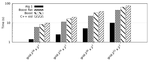
(a) Log-plot runtime on grid graphs.

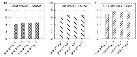
(b) Runtime ratio ($T_{\text{hash}}/T_{\text{array}}$) on grid graphs.

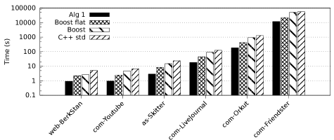
(c) Log-plot runtime on real-world graphs.

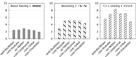
(d) Runtime ratio ($T_{\text{hash}}/T_{\text{array}}$) on real-world graphs.

Figure 3: Array (Algorithm 1) versus hash table (Algorithm 6) for counting $\lozenge(G)$.

Next we show in Figure 4 that our array-based Algorithm 3 for computing 4-cycle counts on each vertex also outperforms the corresponding hash table implementation given in Algorithm 7. Unlike our hash-based Algorithm 6, we cannot skip the second pass over the graph in Algorithm 7. We remind the reader that the current methods [27, 28, 32, 29] also take more than one pass. For Algorithm 3 we implemented the array $L$ to hold pairs of integers in order to double buffer the counts of $y$ in the degree-oriented path $(v,u,y)$. This is more cache-friendly than allocating two separate arrays. We also tested using pairs holding an integer and Boolean, where the Boolean value was used to flag when to reset the counts in the first pass. But we did not observe significant performance gain despite this approach being more space-efficient.

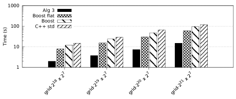
(a) Log-plot runtime on grid graphs.

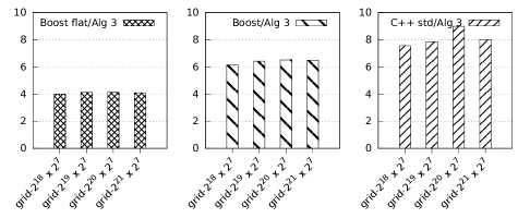
(b) Runtime ratio ($T_{\text{hash}}/T_{\text{array}}$) on grid graphs.

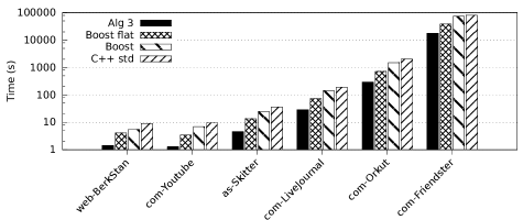
(c) Log-plot runtime on real-world graphs.

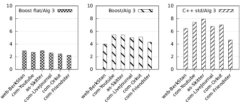
(d) Runtime ratio ($T_{\text{hash}}/T_{\text{array}}$) on real-world graphs.

Figure 4: Array (Algorithm 3) versus hash table (Algorithm 7) for counting $\lozenge(v)$.

Finally, Figure 5 gives a comparison of runtime performance for edge-local 4-cycle counting, showing that our array-based Algorithm 4 is faster than the corresponding hash table implementation given in Algorithm 8. The timing for Algorithm 4 includes the set-up time to construct the prefix-sum array $T$. The hash table on edges uses a 64-bit integer key, and for each edge $\{u,v\}$ we stored the endpoint that sorted first in the higher-order 32 bits of the key and the other endpoint in the lower remaining bits.

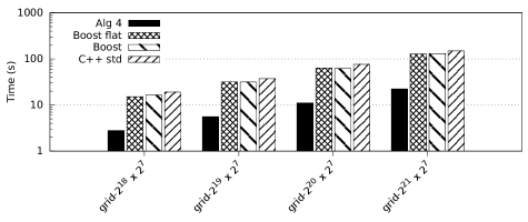
(a) Log-plot runtime on grid graphs.

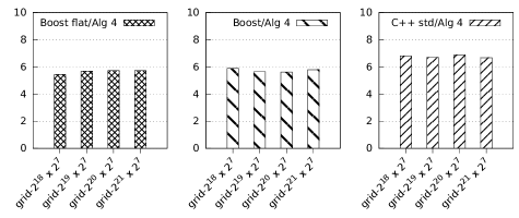
(b) Runtime ratio ($T_{\text{hash}}/T_{\text{array}}$) on grid graphs.

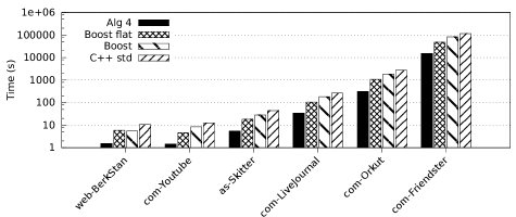
(c) Log-plot runtime on real-world graphs.

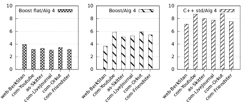
(d) Runtime ratio ($T_{\text{hash}}/T_{\text{array}}$) on real-world graphs.

Figure 5: Array (Algorithm 4) versus hash table (Algorithm 8) for counting $\lozenge(e)$.

There are many optimizations that could potentially improve the performance of either the array or hash table based implementations. Our motivation here is to provide supporting evidence that our simple array-based approach is an appealing alternative to the current hash-based methods.

Appendix A Hash table derivatives of Algorithm 1

In our Algorithm 1, the $L$ table is a flat array of integers in order to ensure deterministic performance. In other approaches, e.g. [28, 29], a hash table is used instead. On one hand, a hash table may use less memory on average (depending on the actual number of vertices indexed); on the other hand, a hash table has higher overhead due to collisions, etc.

There is a particularly clean variant of Algorithm 1 using hash tables, which we describe as follows:

Algorithm 6 4-cycle counting with hash tables

1:for $v\in V$ do

2:     Initialize a zero-filled hash-table $H$ indexed by $V$

3:     for $u\in N(v)$ do

4:         if $u\prec v$ then

5:              for $y\in N(u)$ do

6:                  if $y\prec v$ then

7:                       set $\lozenge(G)\coloneqq\lozenge(G)+H(y)$

8:                       set $H(y)\coloneqq H(y)+1$                                               

This requires just a single pass for each vertex $v$, in contrast to previous algorithms [27, 28, 32, 29]; instead of explicitly zeroing out the hash table $H$, we can simply discard it and re-initialize for the next vertex $v$.

Along similar lines, replacing the $L$ array with a hash table in Algorithm 3 yields the following hash-based, vertex-local 4-cycle counting algorithm.

Algorithm 7 Hash-based Vertex-local 4-cycle counting

1:zero-initialized array $\lozenge$ of size $n$ indexed by $V$

2:for $v\in V$ do

3:     Initialize a zero-filled hash table $H$ indexed by $V$

4:     for $u\in N(v)$ do

5:         if $u\prec v$ then

6:              for $y\in N(u)$ do

7:                  if $y\prec v$ then

8:                       set $\lozenge(v):=\lozenge(v)+H(y)$

9:                       set $\lozenge(y):=\lozenge(y)+H(y)$

10:                       set $H(y)\coloneqq H(y)+1$                                               

11:     for $u\in N(v)$ do

12:         if $u\prec v$ then

13:              for $y\in N(u)$ do

14:                  if $y\prec v$ then

15:                       set $\lozenge(u)\coloneqq\lozenge(u)+H(y)-1$                                               

We can extend Algorithm 3 to compute the 4-cycle counts on each edge; see Algorithm 8 for details. This does not directly give Theorem 3, due to the use of a randomized data structure. We emphasize that whenever the hash table on edges $H_{e}$ is accessed we sort the edge endpoints to get the correct count for the unordered endpoint pair $\{x,y\}$.

Algorithm 8 Hash-based Edge-local 4-cycle counting

1:zero-initialized hash table $H_{v}$ of size $n$

2:zero-initialized hash table $H_{e}$ of size $m$

3:for $v\in V$ do

4:     for $u\in N(v)$ do

5:         if $u\prec v$ then

6:              for $y\in N(u)$ do

7:                  if $y\prec v$ then

8:                       set $H_{v}(y)\coloneqq H_{v}(y)+1$                                               

9:     for $u\in N(v)$ do

10:         if $u\prec v$ then

11:              for $y\in N(u)$ do

12:                  if $y\prec v$ then

13:                       set $H_{e}(\{v,u\})\coloneqq H_{e}(\{v,u\})+H_{v}(y)-1$

14:                       set $H_{e}(\{u,y\})\coloneqq H_{e}(\{u,y\})+H_{v}(y)-1$                                               

In Algorithm 8 we update $H_{e}(\{v,u\}),H_{e}(\{u,y\})$ in the second iteration for similar reasons why we updated $\lozenge(u)$ in the second iteration of Algorithm 3. Namely, since $u$ is the intersecting vertex in the $(v,u,y)$ path for a 4-cycle, then $u$ is in $H_{v}(y)-1$ cycles involving the endpoints $v,y$ and hence the final count of $H_{v}(y)$ is needed.

Appendix B Wallclock times

B.1 Algorithm 1 and hash-based Algorithm 6 for counting $\lozenge(G)$

Table 3: Wallclock time in seconds for counting $\lozenge(G)$.

		Algorithm 6
	Algorithm 1	Boost Flat	Boost	C++ std
grid-$2^{18}\times 2^{7}$	1.41	5.95	8.28	9.85
grid-$2^{19}\times 2^{7}$	2.51	11.26	16.53	19.57
grid-$2^{20}\times 2^{7}$	5.16	22.61	33.02	39.11
grid-$2^{21}\times 2^{7}$	10.00	45.21	65.36	78.07
web-BerkStan	0.92	2.23	2.61	5.13
com-Youtube	0.94	2.37	4.71	6.53
as-Skitter	2.80	8.09	14.87	23.18
com-LiveJournal	17.52	44.70	91.05	123.69
com-Orkut	181.80	430.05	932.83	1296.50
com-Friendster	11680.59	22339.08	50641.69	56099.33

B.2 Algorithm 3 and hash-based Algorithm 7 for counting $\lozenge(v)$

Table 4: Wallclock time in seconds for counting $\lozenge(v)$.

		Algorithm 7
	Algorithm 3	Boost Flat	Boost	C++ std
grid-$2^{18}\times 2^{7}$	1.97	7.90	12.11	14.93
grid-$2^{19}\times 2^{7}$	3.74	15.41	23.98	29.34
grid-$2^{20}\times 2^{7}$	7.35	30.35	47.85	66.07
grid-$2^{21}\times 2^{7}$	14.79	60.51	95.91	118.37
web-BerkStan	1.40	4.08	5.56	9.02
com-Youtube	1.27	3.43	6.96	9.45
as-Skitter	4.59	13.48	24.81	36.42
com-LiveJournal	28.34	73.62	142.10	191.51
com-Orkut	292.13	713.07	1490.45	2044.30
com-Friendster	17370.65	38427.78	74335.70	80277.22

B.3 Algorithm 4 and hash-based Algorithm 8 for counting $\lozenge(e)$

Table 5: Wallclock time in seconds for counting $\lozenge(e)$.

		Algorithm 8
	Algorithm 4	Boost Flat	Boost	C++ std
grid-$2^{18}\times 2^{7}$	2.80	15.18	16.46	19.04
grid-$2^{19}\times 2^{7}$	5.58	31.65	31.51	37.38
grid-$2^{20}\times 2^{7}$	11.08	63.48	62.23	76.16
grid-$2^{21}\times 2^{7}$	22.28	127.71	128.99	148.67
web-BerkStan	1.50	5.86	5.48	10.71
com-Youtube	1.44	4.52	8.45	12.51
as-Skitter	5.49	18.11	28.01	43.92
com-LiveJournal	34.32	104.60	181.84	265.44
com-Orkut	314.22	1078.08	1852.63	2751.60
com-Friendster	15211.27	47820.85	82507.84	114516.72

References

- [1] A. Abboud, K. Bringmann, and N. Fischer. Stronger 3-SUM lower bounds for approximate distance oracles via additive combinatorics. In Proceedings of the 55th annual ACM Symposium on Theory of Computing (STOC), pages 391–404, 2023.
- [2] A. Abboud, S. Khoury, O. Leibowitz, and R. Safier. Listing 4-cycles. arXiv 2211.10022, 2022.
- [3] J. Alman and V. V. Williams. A refined laser method and faster matrix multiplication. In Proceedings of the 2021 ACM-SIAM Symposium on Discrete Algorithms, SODA’21, pages 522–539, 2021.
- [4] N. Alon, R. Yuster, and U. Zwick. Finding and counting given length cycles. In European Symposium on Algorithms, ESA ’94, pages 354–364, 1994.
- [5] N. Alon, R. Yuster, and U. Zwick. Color-coding. Journal of the ACM, 42(4):844–856, 1995.
- [6] N. Alon, R. Yuster, and U. Zwick. Finding and counting given length cycles. Algorithmica, 17:209–223, 1997.
- [7] J.-P. Aumasson and D. J. Bernstein. SipHash: a fast short-input PRF. In International Conference on Cryptology in India, pages 489–508. Springer, 2012.
- [8] J. A. Bondy and M. Simonovits. Cycles of even length in graphs. Journal of Combinatorial Theory, Series B, 16(2):97–105, 1974.
- [9] Boost. Boost C++ Libraries. https://www.boost.org/doc/libs/1_82_0/libs/unordered/doc/html/unordered.html, April 2023.
- [10] P. Burkhardt. Triangle centrality. arXiv 2105.00110, 2021.
- [11] P. Burkhardt, V. Faber, and D. G. Harris. Bounds and algorithms for graph trusses. Journal of Graph Algorithms and Applications, 24(3):191–214, 2020.
- [12] N. Chiba and T. Nishizeki. Arboricity and subgraph listing algorithms. SIAM Journal on Computing, 14(1):210–223, 1985.
- [13] J. Cohen. Graph twiddling in a MapReduce world. Computing in Science and Engineering, 11(4):29–41, 2009.
- [14] S. A. Crosby and D. S. Wallach. Denial of service via algorithmic complexity attacks. In 12th USENIX Security Symposium (USENIX Security 03), 2003.
- [15] D. Ediger, R. McColl, J. Riedy, and D. A. Bader. STINGER: High performance data structure for streaming graphs. In 2012 IEEE Conference on High Performance Extreme Computing, pages 1–5. IEEE, 2012.
- [16] A. Friggeri, G. Chelius, and E. Fleury. Triangles to capture social cohesion. In 2011 IEEE Third International Conference on Social Computing, pages 258–265, 2011.
- [17] T. Hočevar and J. Demšar. Combinatorial algorithm for counting small induced graphs and orbits. PloS one, 12(2):e0171428, 2017.
- [18] C. Jin and Y. Xu. Removing additive structure in 3sum-based reductions. In Proceedings of the 55th annual ACM Symposium on Theory of Computing (STOC), pages 405–418, 2023.
- [19] W. Khaouid, M. Barsky, V. Srinivasan, and A. Thomo. K-core decomposition of large networks on a single PC. Proceedings of the VLDB Endowment, 9(1):13–23, 2015.
- [20] A. Kyrola, G. Blelloch, and C. Guestrin. GraphChi: Large-scale graph computation on just a PC. In Proceedings of the 10th USENIX Conference on Operating Systems Design and Implementation, OSDI’12, page 31–46, 2012.
- [21] M. Leitner-Ankerl. Hashmaps benchmarks - overview. https://martin.ankerl.com/2019/04/01/hashmap-benchmarks-01-overview/, 2019.
- [22] J. Leskovec and A. Krevl. SNAP Datasets: Stanford large network dataset collection. http://snap.stanford.edu/data, June 2014.
- [23] L. Ma, Z. Yang, H. Chen, J. Xue, and Y. Dai. Garaph: Efficient gpu-accelerated graph processing on a single machine with balanced replication. In Proceedings of the 2017 USENIX Conference on Usenix Annual Technical Conference, USENIX ATC ’17, page 195–207, 2017.
- [24] S. Maass, C. Min, S. Kashyap, W. Kang, M. Kumar, and T. Kim. Mosaic: Processing a trillion-edge graph on a single machine. In Proceedings of the 12th European Conference on Computer Systems, EuroSys ’17, page 527–543, 2017.
- [25] H. Park, J. Xiong, and M.-S. Kim. Trillion-scale graph processing simulation based on top-down graph upscaling. In 2021 IEEE 37th International Conference on Data Engineering, ICDE ’21, pages 1512–1523, 2021.
- [26] A. Pinar, C. Seshadhri, and V. Vishal. ESCAPE: Efficiently counting all 5-vertex subgraphs. In Proceedings of the 26th International Conference on World Wide Web, pages 1431–1440, 2017.
- [27] S.-V. Sanei-Mehri, A. E. Sariyüce, and S. Tirthapura. Butterfly counting in bipartite networks. In Proceedings of the 24th ACM SIGKDD International Conference on Knowledge Discovery and Data Mining, KDD ’18, pages 2150–2159, 2018.
- [28] K. Wang, X. Liu, L. Qin, W. Zhang, and Y. Zhang. Vertex priority based butterfly counting for large-scale bipartite networks. Proceedings of the VLDB Endowment, 12(10):1139–1152, 2019.
- [29] K. Wang, X. Liu, L. Qin, W. Zhang, and Y. Zhang. Accelerated butterfly counting with vertex priority on bipartite graphs. The VLDB Journal, 2022.
- [30] D. J. Watts and S. H. Strogatz. Collective dynamics of ‘small-world’ networks. Nature, 393(6684):440–442, 1998.
- [31] V. V. Williams, J. R. Wang, R. Williams, and H. Yu. Finding four-node subgraphs in triangle time. In Proc. 26th annual ACM-SIAM Symposium on Discrete Algorithms (SODA), pages 1671–1680, 2015.
- [32] A. Zhou, Y. Wang, and L. Chen. Butterfly counting on uncertain bipartite graphs. Proceedings of the VLDB Endowment, 15(2):211–223, 2021.