Quantum formalism for cognitive psychology

Abstract

The cognitive state of mind concerning a range of choices to be made can effectively be modelled in terms of an element of a high-dimensional Hilbert space. The dynamics of the state of mind resulting form information acquisition is characterised by the von Neumann-Lüders projection postulate of quantum theory. This is shown to give rise to an uncertainty-minimising dynamical behaviour equivalent to the Bayesian updating, hence providing an alternative approach to characterising the dynamics of cognitive state that is consistent with the free energy principle in brain science. The quantum formalism however goes beyond the range of applicability of classical reasoning in explaining cognitive behaviours, thus opens up new and intriguing possibilities.

Introduction

The present paper is concerned with the use of Hilbert space techniques, so successfully implemented in characterising behaviours and properties of quantum systems Isham , to model cognitive ‘psychology’ in the sense to be defined below. The paper, on the other, is not concerned with whether quantum effects, such as interference, violation of the Bell inequality, or the use of complex numbers, might play a role in psychology or in brain activities. There are differing opinions on the matter Penrose ; Vitiello ; Tegmark ; Plotnitsky ; Ozawa , but these will not be addressed here, for, the use of Hilbert space techniques in modelling cognitive behaviour, in themselves, do not necessarily require functioning of brain neurophysiology to be quantum mechanical. What does concern us will include the tensor product structure of the Hilbert space, entanglements, the superposition principle, the projection postulate, and decoherence. While some may view these to be intrinsically quantum-mechanical effects, I will show that they are in fact intrinsic to any probabilistic system modelled on a Hilbert space — an idea that dates back to the pioneering work of Rao Rao . At any rate, my purpose here is to illustrate how it is both natural and effective to implement Hilbert space techniques in modelling cognitive human behaviours. Such a proposal, in itself, is not new (see, e.g., Busemeyer ; Busemeyer2 and references cited therein). My main contribution is to introduce a formalism that allows for a systematic treatment of the dynamics of cognitive state of mind, from which predictions can be made.

The key idea to be explored is that the state of mind of a person, to be defined more precisely, can efficiently be represented in terms of a vector in a high-dimensional Hilbert space, which in turn is a tensor product of lower-dimensional Hilbert spaces. However, before turning to technical discussion, I would like to illustrate the significance of the superposition principle in this context through simple examples. The first concerns the tossing of a fair coin. When a coin is tossed, but the outcome not yet revealed, no one will dispute the state of the coin, which is a macroscopic classical object: it is either in the ‘head’ state or in the ‘tale’ state. In fact, even before the coin is tossed, it will be known to all that the state of the coin will be either head or tail. However, a person who is in the position to guess the outcome is having a different state of mind. Until the moment when a choice is made, the person’s mind is in the state of neither head nor tail – it is in a state of a superposition. Thus there is a dissonance between the objective reality of the state of the coin and the state of the mind attempting to determine the state of the coin.

Another example is seen in children’s hand game of rock, scissors and paper. Again, until the last moment when the decision is made as to which hand to choose, the person’s mind is in the state of a superposition between the three alternatives. Of course, with any decision, a person may come with a predetermined outcome — as in Groucho Marx’s whatever it is, I’m against it! But until when that decision is made, the fact remains that the mind is in an indefinite state. Only at the moment when the decision is made, for example to declare that the outcome of the coin tossing is head, or choosing the scissors hand, the state ‘collapses’ into one of the definite states. This situation is very much analogous to the measurement process in quantum theory.

With these heuristics in mind, the present paper will be organised as follows. I begin by defining what I mean by the state of mind, which essentially will be a Hilbert-space representation of the probability assignments to the totality of choices available to the person. A given set of choices will then be modelled as an observable acting on this Hilbert space. The idea I put forward is closely related to the proposal made by Busemeyer and his collaborators Busemeyer0 , and that by Khrennikov and his collaborators Khrennikov . One difference to the latter, however, is that I model cognitive behaviours directly using the quantum formalism, rather than starting from the quantum theory and then deduce implications in behavioural modelling by reduction. As a consequence, I am able to gain certain insights into human behaviour that go beyond what is commonly understood in cognitive psychology. I examine how the state of mind changes when a person acquires noisy information that is relevant to decision making. My approach will be consistent with the cybernetics framework of Wiener as an attempt to understand the dynamics of living systems Wiener . I will use the von Neumann-Lüders projection postulate in quantum mechanics to arrive at the change in the state of mind, and show that the result agrees with the classical formulation using the Bayes formula; in agreement with related previous findings Khrennikov . Further, I show that the projection postulate gives rise to an evolution that on average minimises future ‘surprises’, and hence is consistent with the free-energy principle widely adopted in brain science Friston0 . I then consider what happens when noisy information arrives in continuous time. When the dynamical evolution of the state of mind resulting from a sequential von Neumann-Lüders projection postulate is reduced to a projective Hilbert space, the dynamical equation reveals an important feature, namely, that each state of zero uncertainty, having vanishing Shannon-Wiener entropy, acts as an attractor to the dynamics. The result provides a geometric explanation of certain characteristics of human behaviour seen in psychology literature (such as confirmation bias), which I have previously called the tenacious Bayesian behaviour Brody2 . The work presented here demonstrates the fact that if a person’s opinion is strongly skewed towards one of the false alternatives, and if all choice observables are commutative, then even if partial information about the truth is revealed and the person behaves rationally in accordance with Bayesian updating, it is very difficult for the person to escape from the initial misconception. In other words, adherences to false narratives commonly observed in today’s society is not due to irrational behaviours. Following the proposal in Busemeyer , I then consider what happens if choice observables are not commutative. This is motivated by the observation that many empirical observations concerning cognitive human behaviours cannot be fully described by use of a commuting set of observables. The existence of incompatible observables can be used to rescue a person fallen into a false attractor; a possibility that is unavailable by use of purely classical reasonings.

Decision making and the state of mind

Throughout the paper I will be concerned with the cognitive process of decision making, which will be a topic distinct from what is known as statistical decision theory, for which there are excellent treatise DeGroot ; Berger . A decision making occurs when a person is unsure from which alternative to choose; but I will be using the term ‘decision making’ in a broad sense to include a person’s uncertain point of view on a topic, for which there are multiple views, and for which there may not be a need to choose one particular alternative. At any rate, this uncertainty, which is largely due to lack of sufficient information, can be modelled in the form of a set of probabilities that represents the likelihoods of different alternatives being selected. Suppose that a decision needs to be made to choose one out of $N$ alternatives. (The number of alternatives can be infinite, or even uncountable — the formalism extends naturally to these cases, but for simplicity I will consider the finite case here.) At a given moment in time, let $p_{k}$ denote the likelihood that the $k$th alternative is selected. If $p_{k}=1$ for a value of $k$ then the mind is in a definite state in relation to this decision. Hence for a given decision, the set of numbers $(p_{1},p_{2},\ldots,p_{N})$ represents the state of mind in relation to that decision making.

Of course, at any moment in time one faces a multitude of decisions, not just one, some of which are intertwined with each other while others are independent. In probability theory, such a situation is modelled by means of a joint probability for the totality of decisions. Alternatively, though equivalent, the situation can be modelled on a Hilbert space by use of the square-root map: $p_{k}\to\psi_{k}=\sqrt{p_{k}}$. Clearly, the vector with components $\{\psi_{k}\}$, in the basis $|e_{k}\rangle=(0,0,0,\ldots,1,0,\ldots,0)$ with only the $k$th element nonzero, is an element of an $N$-dimensional real Hilbert space ${\cal H}^{N}$. Thus, in terms of the Dirac notation the state can be expressed in the form of a superposition $|\psi\rangle=\sum_{k}\psi_{k}|e_{k}\rangle$. If there is a second decision to be made out of $M$ alternatives, then the state of a person’s mind in relation to these two choices is represented by an element of the tensor product ${\cal H}^{N}\otimes{\cal H}^{M}$. This tensor product structure arises solely from statistical dependencies of two decisions, when modelled on a Hilbert space.

This construction extends for an arbitrary number of decisions to be made. With this in mind, I define the state of mind of a person facing a range of alternatives to consider, at any moment in time, to be an element of the tensor product ${\cal H}=\otimes_{l=1}^{K}{\cal H}_{l}$, where $K$ is the number of distinct decisions. If two decisions can be made independently, then the component of the state vector belonging to the corresponding subspace of ${\cal H}$ will be in a product state. Otherwise, a state is entangled. As a simple example, consider a pair of binary decisions, for example, whether to take fish or meat for the main course, and whether to take red or white wine to accompany the dinner. Writing $|F\rangle$ and $|M\rangle$ for the food choices, and similarly $|R\rangle$ and $|W\rangle$ for the wine selections, if the state of mind of a person is $|\psi\rangle=c_{1}|FW\rangle+c_{2}|MR\rangle$, then the person will choose fish with white wine with probability $c_{1}^{2}$, and meat with red wine with probability $c_{2}^{2}=1-c_{1}^{2}$; but no other option will be chosen. This is evidently an entangled state, which collapses to one or the other alternatives at the moment (or before) the waiter arrives and takes the order.

In this Hilbert space formulation, a given choice can be modelled by a real symmetric matrix, whose dimension is the number of alternatives. Such a matrix corresponds to observables in quantum mechanics. I will assume, for now, that all such ‘observables’ or ‘choices’ are compatible in the sense that the matrix representations can be diagonalised simultaneously. What this means is that at any given time, an arbitrary number of decisions can be made simultaneously. It is then evident that no state of mind, whether entangled or not, can violate laws of classical probability, and hence no state can violate, in particular, Bell’s inequalities. Later in the paper, however, I will consider the case where choice observables are incompatible.

The eigenvalues of choice observables then label different alternatives. This is analogous to quantum observables when it concerns labelling outcomes of a single measurement. However, observables in quantum theory have a second role apart from representing measurement outcomes: they generate dynamics. As a consequence, the differences of observable eigenvalues have direct physical consequences, and hence they cannot be chosen arbitrarily. It appears, in contrast, that the differences of eigenvalues of the choice observables have no significance: the results of a selection, such as choosing a hand in the game of rock, scissors and paper, can be labelled by means of any three distinct numerical values, merely as place keepers so that statistical analysis can be applied. It will be shown below, however, that when it concerns the dynamics of the state of mind, the eigenvalue differences do play an important role, and hence they cannot be chosen arbitrarily, just as in quantum theory.

Dynamics

Having established the framework for representing the cognitive state of mind, it will be of interest to explore how the state changes in time. To this end I will be working under the hypothesis that a given state $|\psi\rangle$ of a person’s mind changes only by transfer of information. It is, of course, possible that an isometric motion analogous to unitary motion of quantum theory that does not exchange information can change the state, and if so this will be given by an orthogonal transformation. However, without a clear physical or psychological evidence indicating the existence of such a symmetry, I will not consider this possibility, and focus instead on universally acknowledged empirical fact that information acquisition (or loss) changes states of minds. The question is, in which way?

To understand dynamics, I will be borrowing ideas from communication theory. Focusing on a single decision to start with, let ${\hat{X}}$ denote the decision or choice observable, with eigenvalues $\{x_{k}\}_{k=1,\ldots,N}$. These eigenvalues for now merely label different alternatives. The eigenstate $|x_{j}\rangle$ of ${\hat{X}}$, satisfying ${\hat{X}}|x_{j}\rangle=x_{j}|x_{j}\rangle$, thus represents the state of mind in which the $j$th alternative has been chosen. Prior to an alternative being chosen, the state is in a superposition $|\psi\rangle=\sum_{k}c_{k}|x_{k}\rangle$. The state will change when the person acquires information relevant to decision making. This information is rarely perfect. In communication theory, anything that obscures finding the value of the quantity of interest is modelled in terms of noise. Let ${\hat{\varepsilon}}$ denote this noise. Here, ${\hat{\varepsilon}}$ can take discrete values, or more commonly continuous values. I will consider the latter case so that ${\hat{\varepsilon}}$ acts on an infinite dimensional Hilbert space ${\cal H}^{\infty}$ distinct from the state space ${\cal H}^{N}$. The noise arises from external environments ${\cal E}$. For simplicity I will assume that the state of noise is pure, and is given by $|\eta\rangle=\eta(y)\in{\cal H}^{\infty}$, although a mixed state can equally be treated. Then initially the state of mind of a person attempting to make a decision and the state of the noise-inducing environment is disentangled, and together is given by the product state $|\psi\rangle|\eta\rangle$.

Acquisition of partial information relevant to decision making can then be modelled by observing the value of

$${\hat{\xi}}={\hat{X}}+{\hat{\varepsilon}}.$$

Here, the sum is taken in the tensor-product space ${\cal H}^{N}\otimes{\cal H}^{\infty}$. To understand the sum, consider the case in which ${\hat{\varepsilon}}$ is finite and can take three values $\varepsilon_{1},\varepsilon_{2},\varepsilon_{3}$, while the decision is binary, represented by the values $x_{0}$ and $x_{1}$. Then ${\hat{\xi}}$ is a $6\times 6$ matrix with the eigenvalues $x_{0}+\varepsilon_{1}$, $x_{0}+\varepsilon_{2}$, $x_{0}+\varepsilon_{3}$, $x_{1}+\varepsilon_{0}$, $x_{1}+\varepsilon_{1}$, $x_{1}+\varepsilon_{3}$. In general, the eigenvalues of ${\hat{\xi}}$ are highly (typically $N$-fold) degenerate. The form that ${\hat{\xi}}$ takes is of course nothing more than a signal-plus-noise decomposition in classical communication theory Wiener . The ‘signal’ term, more generally, will be a function $F({\hat{X}})$ of ${\hat{X}}$, but for simplicity I will assume the function to be linear because the choice of $F(x)$ is context dependant.

Once the value of the information-providing observable ${\hat{\xi}}$ is measured, the initially-disentangled state

$$|\psi\rangle|\eta\rangle=\sum_{k}\sqrt{p_{k}}\,\eta(y)|x_{k}\rangle$$

becomes an entangled state. In quantum mechanics, the transformation of the state after measurement is given by the von Neumann-Lüders projection postulate. That is, writing

$${\hat{\Pi}}_{\xi}=\sum_{k}\delta(y-\xi+x_{k})|x_{k}\rangle\langle x_{k}|$$

for the projection operator onto the subspace of ${\cal H}^{N}\otimes{\cal H}^{\infty}$ spanned by the eigenstates of ${\hat{\xi}}$ with the eigenvalue $\xi$, the projection postulate asserts that the state of the system after information acquisition is

$${\hat{\rho}}_{\xi}=\frac{{\hat{\Pi}}_{\xi}|\psi\rangle|\eta\rangle\langle\psi|\langle\eta|{\hat{\Pi}}_{\xi}}{{\rm tr}\left({\hat{\Pi}}_{\xi}|\psi\rangle|\eta\rangle\langle\psi|\langle\eta|{\hat{\Pi}}_{\xi}\right)}.$$

A short calculation then shows that this is given more explicitly by

$${\hat{\rho}}_{\xi}=\frac{\sum_{k,l}\sqrt{p_{k}p_{l}}\,\eta(\xi-x_{k})\eta(\xi-x_{l})\,|x_{k}\rangle\langle x_{l}|}{\sum_{m}p_{m}\eta^{2}(\xi-x_{m})}.$$

Two interesting observations that follow are in order. First, the density matrix by construction is a projection operator onto a random pure state $|\psi(\xi)\rangle$ given by

$$|\psi(\xi)\rangle=\sum_{k}\sqrt{\pi_{k}(\xi)}\,|x_{k}\rangle,$$

where $\xi$ is the random variable with the density $p(y)=\sum_{m}p_{m}\eta^{2}(y-x_{m})$ modelled by the observable ${\hat{\xi}}$ along with the initial state $|\psi\rangle|\eta\rangle$. That is, given the state $|\psi\rangle|\eta\rangle$, the probability of the measurement outcome of the observation lying in the interval $[y,y+\mbox{$\rm d$}y]$ is given by $p(y)\mbox{$\rm d$}y$. Second, the coefficients of the random pure state agrees with the conditional probability of the choice given by the Bayes formula:

$$\pi_{k}(\xi)=\frac{p_{k}\,\eta^{2}(\xi-x_{k})}{\sum_{m}p_{m}\eta^{2}(\xi-x_{m})}.$$

That is, $\pi_{k}(\xi)$ is the probability that the $k$th alternative is chosen, conditional on observing the value $\xi$ of ${\hat{\xi}}$. It follows that the von Neumann-Lüders projection postulate of quantum theory not only gives the correct classical result (as already observed in Ozawa ; Khrennikov with a different construction) but also provides a simple geometric interpretation of the Bayes formula. This follows because the Lüders state $|\psi(\xi)\rangle$ associated to a degenerate measurement outcome $\xi$ is given by the orthogonal projection of the initial state onto Hilbert subspace associated to this outcome. Hence $|\psi(\xi)\rangle$ is the closest state on the constrained subspace in terms of the Bhattachayya distance BH to the initial state $|\psi\rangle|\eta\rangle$.

It is worth remarking that an alternative interpretation of the von Neumann-Lüders projection postulate can be given in terms of the so-called free energy principle KF1 . Intuitively, this principle asserts that the change in the state of mind follows a path that on average minimises elements of surprises. In the present context, the degree of surprise can be measured in terms of the level of uncertainty. Suppose that the state of mind after information acquisition becomes ${\hat{\mu}}_{\xi}$ that is different from the Lüders state ${\hat{\rho}}_{\xi}$. Then the level of uncertainty associated with the choice observable ${\hat{X}}$ resulting from ${\hat{\mu}}_{\xi}$, conditional on the observed value $\xi$ of ${\hat{\xi}}$, is given by

$${\rm tr}\left(\left[{\hat{X}}-{\rm tr}({\hat{X}}{\hat{\mu}}_{\xi})\right]^{2}{\hat{\rho}}_{\xi}\right)={\rm tr}\left({\hat{X}}^{2}{\hat{\rho}}_{\xi}\right)-\left({\rm tr}\left({\hat{X}}{\hat{\rho}}_{\xi}\right)\right)^{2}+\left({\rm tr}\left({\hat{X}}{\hat{\delta}}_{\xi}\right)\right)^{2},$$

where I have written ${\hat{\delta}}_{\xi}={\hat{\mu}}_{\xi}-{\hat{\rho}}_{\xi}$ for the deviation. Because the first two terms on the right side is the conditional variance of ${\hat{X}}$, which is positive and is independent of ${\hat{\mu}}_{\xi}$, to minimise the expected uncertainty, and hence the surprise, for all ${\hat{X}}$ and $\xi$, it has to be that ${\hat{\delta}}_{\xi}=0$. It follows that among all the states consistent with the observation, Lüders state is unique in that it minimises the expected level of future surprise, as measured by the uncertainty.

I might add parenthetically that a psychologist wishing to predict the statistics of the behaviour of a person who has acquired information relevant to decision making will a priori not know the observed value of $\xi$. Hence in this case the density matrix ${\hat{\rho}}_{\xi}$ has to be averaged over $\xi$, but the denominator of ${\hat{\rho}}_{\xi}$ is just the density $p(y)$ for $\xi$, so the averaged density matrix is given by

$${\mathbb{E}}[{\hat{\rho}}_{\xi}]=\sum_{k,l}\sqrt{p_{k}p_{l}}\,\Lambda(\omega_{kl})\,|x_{k}\rangle\langle x_{l}|,$$

where $\omega_{kl}=x_{k}-x_{l}$ and

$$\Lambda(\omega)=\int_{-\infty}^{\infty}\eta(y)\eta(y-\omega)\mbox{$\rm d$}y.$$

Evidently, $0\leq\Lambda(\omega_{kl})\leq 1$ and $\Lambda(\omega_{kk})=1$ for all $k,l$, but because the initial state of mind $|\psi\rangle\langle\psi|$ in this basis has the matrix elements $\{\!\sqrt{p_{k}p_{l}}\}$, it follows that an external observer (e.g., a psychologist) will perceive a decoherence effect whereby the off-diagonal elements of the reduced density matrix are damped.

It is at this point that I wish to comment on the numerical values of the differences $\{\omega_{kl}\}$. While there is no reason why $\Lambda(\omega)$ should be monotonic in $\omega$ (unless $\eta(y)$ is unimodal), it will certainly be the case that the decoherence effect is more pronounced for large values of $\omega$. That is, $\Lambda(\omega)\ll 1$ for $\omega\gg 1$. For the same token, the values of $\omega_{kl}$ will directly affect the conditional probabilities $\{\pi_{k}(\xi)\}$. Therefore, while the values of $\omega_{kl}$, and hence those of $x_{k}$, can be chosen arbitrarily to describe the statistics of the initial state of mind, once dynamics is taken into account (what happens after information acquisition), it becomes evident that they cannot be chosen arbitrarily.

A better intuition behind this observation can be gained by reverting back to ideas of signal detection in communication theory. For this purpose, consider a binary decision. Supposed that the two eigenvalues of ${\hat{X}}$, labelling the two decisions, are chosen to be, say, $\pm 0.1$ and suppose that the noise distribution $\eta^{2}(y)$ is normal centred at zero, with a small standard deviation. In this case, observed outcomes of ${\hat{\xi}}$ will most likely take values close to zero. As a consequence, a single observation of ${\hat{\xi}}$ will reduce on average the initial uncertainty only by a very small amount. In contrast, suppose that the two eigenvalues of ${\hat{X}}$ are chosen to be $\pm 10$, but the noise is the same as before. Then the observation will almost certainly yield the outcome that is close to $+10$ or $-10$. Hence the uncertainty in this case has been reduced to virtually zero after a single observation. This extreme example shows how it is not possible to label different choice alternatives by arbitrary numerical numbers, while at the same time to adequately model the dynamics of the state of mind.

In the event where a model $\eta(y)$ for the state of noisy environment exists, it is possible in principle to estimate the eigenvalue differences $\{\omega_{ij}\}$ by studying how much a person’s views shifted from the acquisition of the noisy information. This is because the average reduction of uncertainty, as measured by entropy change or the decoherence rate, is determined by the eigenvalue differences $\{\omega_{ij}\}$.

Sequential updating

I have illustrated how the cognitive state of mind of a person in relation to a given choice changes after a single acquisition of information. A more interesting, as well as realistic, situation concerns a sequential updating of the state of mind as more and more noisy information is revealed. In this case the information-providing observable ${\hat{\xi}}_{t}$ is a time series. As a simple example that naturally extends the previous one I will consider the following time series

$${\hat{\xi}}_{t}={\hat{X}}t+{\hat{\varepsilon}}_{t},$$

where I will assume that the noise term ${\hat{\varepsilon}}_{t}$ is modelled by a standard Brownian motion $\{B_{t}\}$ multiplied by the identity operator of the Hilbert space ${\cal H}^{\infty}$. The ‘signal’ component, more generally, can be given by $\int_{0}^{t}F_{s}({\hat{X}})\mbox{$\rm d$}s$, but again for simplicity I will assume that the function $F_{t}(x)$ is linear for all $t$. In fact, even more generally, the range of alternatives ${\hat{X}}$ itself can also be time dependent, but I will not consider this case here.

In this example, what happens to the state of mind can be worked out by discretising the time and taking the limit. Starting from time zero, over a small time increment $\mbox{$\rm d$}t$ the initial state $|\psi\rangle|\eta\rangle$ is projected to the Lüders state ${\hat{\Pi}}_{\xi_{{\rm d}t}}|\psi\rangle|\eta\rangle$, suitably normalised, in accordance with the projection postulate. In this case, the noise is normally distributed with mean zero and variance $\mbox{$\rm d$}t$, so that $\eta(y)$ is just the square-root of the corresponding Gaussian density function. Then after another time interval $\mbox{$\rm d$}t$ we apply the projection operator again, and repeat the procedure till time $t$. Finally, taking the limit, a calculation shows that the Lüders state, after monitoring the observable ${\hat{\xi}}_{t}$ up to time $t$, is given by

$$|\psi(\xi_{t})\rangle=\frac{1}{\sqrt{\Phi_{t}}}\sum_{k}\sqrt{p_{k}}\,\mbox{$\rm e$}^{\frac{1}{2}x_{k}\xi_{t}-\frac{1}{4}x_{k}^{2}t}|x_{k}\rangle,$$

where $\xi_{t}=Xt+B_{t}$ and $X$ is the random variable represented on the Hilbert space ${\cal H}^{N}$ by the operator ${\hat{X}}$ along with the initial state $|\psi\rangle$, and $\Phi_{t}=\sum_{k}p_{k}\mbox{$\rm e$}^{\frac{1}{2}k_{k}\xi_{t}-\frac{1}{4}x_{k}^{2}t}$ gives the normalisation.

Because we have an explicit expression that monitors the change in the state of mind as information is revealed, there is a priori no reason to identify the differential equation to which $|\psi(\xi_{t})\rangle$ is the solution. Nevertheless, the exercise of working out the dynamical equation provides several new insights worth discussing. The detailed mathematical steps required here to work out the dynamics has been outlined in BH2 , so I shall not repeat this. It suffices to say that the Lüders state is a function of $t$ and $\xi_{t}$, where the latter is a Brownian motion with a random drift. Hence the relevant calculus to apply is that of Ito: one Taylor expands $|\psi(\xi_{t})\rangle$ in $t$ and $\xi_{t}$, and retain leading-order terms, bearing in mind that $(\mbox{$\rm d$}\xi_{t})^{2}=\mbox{$\rm d$}t$. Then it follows that

$$\mbox{$\rm d$}|\psi(\xi_{t})\rangle=-\frac{1}{8}({\hat{X}}-\langle{\hat{X}}\rangle_{t})^{2}|\psi(\xi_{t})\rangle\,\mbox{$\rm d$}t+\frac{1}{2}({\hat{X}}-\langle{\hat{X}}\rangle_{t})|\psi(\xi_{t})\rangle\,\mbox{$\rm d$}W_{t},$$

where $\langle{\hat{X}}\rangle_{t}=\langle\psi(\xi_{t})|{\hat{X}}|\psi(\xi_{t})\rangle/\langle\psi(\xi_{t})|\psi(\xi_{t})\rangle$ and where

$$\mbox{$\rm d$}W_{t}=\mbox{$\rm d$}\xi_{t}-\langle{\hat{X}}\rangle_{t}\,\mbox{$\rm d$}t.$$

The process $\{W_{t}\}$ defined in this way is in fact a standard Brownian motion, known as the innovations process Kailath . This process has the interpretation of revealing new information. That is, while the time series $\{{\hat{\xi}}_{t}\}$ contains new as well as previously known information about the impending choice to be made, the process $\{W_{t}\}$ merely contains information that was not known previously.

There are two important observations that follow. First, the evolution of the state of mind is not directly generated by the noise $\{B_{t}\}$, nor by the observation $\{\hat{\xi}_{t}\}$. Rather, it is the innovations process that drives the dynamics. But this is the case only if the state of mind changes in such a way to continuously minimise uncertainties. Because the expectation of the cumulative uncertainty is the entropy BH2 , it follows that according to the present framework, the tendency towards low entropy states required in biology KF1 , which forms the basis of the free energy principle, emerges naturally. In particular, the implication here based on the projection postulate is that the state of mind changes only in accordance with the arrival of new information; it will not change spontaneously of its own otherwise. Second, while the analysis presented here can be deduced as a result of standard least-square estimation theory Kailath ; Wonham , I have derived these results using the von Neumann-Lüders projection postulate of quantum theory. It follows that the informationally efficient dynamical behaviour, in the sense of minimising surprises, of a system, is applicable not only to the state of mind but also to quantum systems. An analogous point of view, based on the free energy principle, has recently been proposed elsewhere KF2 .

I might add that for the purpose of psychological modelling, the averaged reduced density matrix ${\hat{\rho}}_{t}={\mathbb{E}}[{\hat{\rho}}_{\xi_{t}}]$ can be seen to obey the dynamical equation

$$\frac{\partial{\hat{\rho}}_{t}}{\partial t}={\hat{X}}{\hat{\rho}}_{t}{\hat{X}}-\frac{1}{2}\left({\hat{X}}^{2}{\hat{\rho}}_{t}+{\hat{\rho}}_{t}{\hat{X}}^{2}\right).$$

This, of course, is just the Lindblad equation generated by the decision ${\hat{X}}$.

Projecting down the dynamics

One advantage of working with the mathematical formalism of quantum theory in modelling psychological states of minds is the deeper insights that it can uncover (cf. Busemeyer ). To this end I note that although I have defined the state of mind as a vector in Hilbert space, what I have in mind really is a projective Hilbert space consisting of rays through the origin of the Hilbert space. The idea is as follows. In probability, one can say, for instance, that the likelihood of an event happening is 0.3, or three out of ten, or 30% — all of these statements convey the same idea. The total probability being equal to one is merely a convenient convention that does not carry any significance. Putting it differently, working with the convention that the expectation of any decision ${\hat{X}}$ in a state $|\psi\rangle$ is given by the ratio $\langle{\hat{X}}\rangle=\langle\psi|{\hat{X}}|\psi\rangle/\langle\psi|\psi\rangle$, it is evident that the expectation values are independent of the overall scaling of the state $|\psi\rangle$ by a nonzero constant. Hence the Hilbert space vector $|\psi\rangle$ carries one psychologically irrelevant degree of freedom. When this degree of freedom is eliminated by the identification $|\psi\rangle\sim\lambda|\psi\rangle$ for any $\lambda\neq 0$, one arrives at a projective Hilbert space, otherwise known as the real projective space. This is a real manifold ${\mathfrak{M}}$ of dimension $N-1$, endowed with a Riemannian metric induced by the underlying probabilistic rules given by the von Neumann-Lüders projection postulate BH4 .

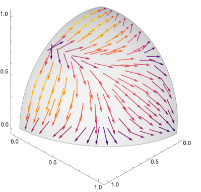
(a) Negative gradient flow of the variance

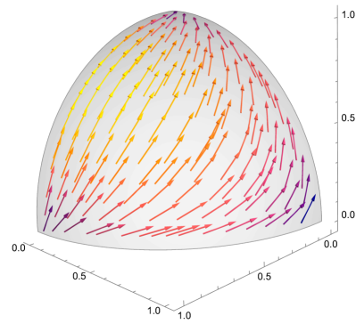
(b) Gradient flow of the mean

Figure 1: Flow of the negative gradient of the variance. In the case of a decision involving three alternatives, the corresponding state space ${\mathfrak{M}}$ is a real projective plane. This two-dimensional manifold is not orientable and cannot be embedded in three dimensions, however, it can be interpreted as a sphere with antipodal points being identified. Thus the flow on ${\mathfrak{M}}$ can be captured by examining the flow on the positive octant of the sphere. Here, a three-fold decision is modelled by a choice observable ${\hat{X}}$ with eigenvalues $x_{1}=1$, $x_{2}=2$, and $x_{3}=3$. The three axes, corresponding to the three corners of the octant, represent the three eigenstates of ${\hat{X}}$ with no uncertainty. The flow $-\nabla^{a}V$ generated by the negative gradient of the uncertainty (shown in the left panel) takes any initial state into one of the states with no uncertainty — this is the tendency towards least surprises. The gradient $\nabla^{a}X$ of the mean is shown on the right panel for comparison. This term is multiplied by the Brownian increment $\mbox{$\rm d$}W_{t}$, which is normally distributed with mean zero and variance $\mbox{$\rm d$}t$, so at any moment in time the direction of the flow generated by the Brownian fluctuation can go either way.

Let $\{\psi^{a}\}$ denote local coordinates for points on ${\mathfrak{M}}$. A point on ${\mathfrak{M}}$ thus represents a state of mind corresponding to a family of vectors $\lambda|\psi\rangle$, $\lambda\neq 0$, on Hilbert space. For any representative $|\psi\rangle$ of that family corresponding to the point $\psi\in{\mathfrak{M}}$, consider a function on ${\mathfrak{M}}$ through the expectation $X(\psi)=\langle\psi|{\hat{X}}|\psi\rangle/\langle\psi|\psi\rangle$. With this convention, and writing $\nabla^{a}$ for the gradient vector, the dynamical equation for the state of mind $|\psi(\xi_{t})\rangle$, when projected down to ${\mathfrak{M}}$, is given by

$$\mbox{$\rm d$}\psi^{a}=-\frac{1}{16}\nabla^{a}V_{X}\,\mbox{$\rm d$}t+\frac{1}{4}\nabla^{a}X\,\mbox{$\rm d$}W_{t},$$

where $V_{X}(\psi)=\langle\psi|({\hat{X}}-X(\psi))^{2}|\psi\rangle/\langle\psi|\psi\rangle$ is the function on ${\mathfrak{M}}$ that corresponds to the variance of ${\hat{X}}$ in the state $|\psi\rangle$. The mathematical analysis leading to this result have essentially been provided in Hughston ; BH3 , which will not be repeated here. The important observation is that the drift term (the coefficient of $\mbox{$\rm d$}t$) that generates a tendency flow on the state space ${\mathfrak{M}}$ is given by the negative gradient of the variance (uncertainty). Therefore, on the state space there is a tendency of driving the state of mind into one of the states with no uncertainty — this is the flow that attempts to reduce surprises. It also follows that if the state of mind is in the vicinity of one of the definite states of no uncertainty, then it will be difficult to escape from that neighbourhood — a phenomenon that I referred to as a tenacious Bayesian behaviour Brody2 . I will have more to comment on this below. In Figure 1 an example of the negative gradient flow of the uncertainty on the state space is sketched, along with the gradient flow $\nabla^{a}X$ of the mean.

It is worth remarking that in principle properties of the dynamics just outlined can be inferred from the squared amplitudes

$$\pi_{kt}=\Phi_{t}^{-1}p_{k}\,\mbox{$\rm e$}^{x_{k}\xi_{t}-\frac{1}{2}x_{k}^{2}t}$$

of the coefficients of $|\psi(\xi_{t})\rangle$, which evidently contain as much information as the state $|\psi(\xi_{t})\rangle$ itself. Indeed, starting from the expression for $\pi_{kt}$, which can be deduced by use of the Bayes formula, one can apply the Ito calculus to deduce the dynamical equation satisfied by $\pi_{kt}$, known in communication theory as the Kushner equation Kushner . However, $\pi_{kt}$ is a martingale, that is, on average a conserved process. In particular, the process has no drift (the coefficient of $\mbox{$\rm d$}t$ in the Kushner equation for $\pi_{kt}$ is zero), so by simply examining the Kushner equation for $\pi_{kt}$ it is difficult to infer key properties of the dynamics. In contrast, the surprise-minimising feature of the dynamics becomes immediately apparent once the process is projected to the state space ${\mathfrak{M}}$.

Difference between psychological and quantum states

I have thus far emphasised the similarities in the state of mind as represented by a Hilbert space vector (or a density matrix), and the physical state of a quantum system as represented by the same scheme. There are, however, some important differences. The most important one, in my view, can be described through the following example. Suppose that the state of a quantum system is very close to one of the eigenstates $|x_{k}\rangle$ of an observable ${\hat{X}}$, and that the measurement outcome yields the value $x_{l}$, $l\neq k$, for which the probability would have been very small. In this case, the interpretation of the event is the obvious one: a rare event has occurred. Now suppose instead that the state of mind is very close to one of the ‘certain’ states $|x_{k}\rangle$, in a situation where there is a correct choice to be made (for example, in deciding what had actually happened at an event in the past — as opposed to choices for which there need not be ‘correct’ outputs). In this case, if the correct choice happens to be $|x_{l}\rangle$, $l\neq k$, it does not mean that an unlikely event had occurred. Rather, it means that the initial state of mind was a misguided one. Putting the matter differently, while a state of a quantum system represents the physical reality of the system, a state of mind merely represents the person’s perception of the state of the world. This difference between objective and subjective probabilities has important implications discussed below. (There is, of course, the suggestion that the state of a quantum system itself is entirely subjective Fuchs , but this idea will not be explored here.)

The subjective nature of psychological states gives rise to the following challenge. In psychology, it is not uncommon for a group of people having varying dispositions be given some information (for example, an article to read or a video clip to watch), and their responses are examined. One such example is seen in the study of confirmation bias — a bias towards information that confirm their views Lord ; Nickerson . The idea is to investigate how people having diverging opinions respond differently to the ‘same’ information. The issue here, however, is that the information content of the given message such as an article or a video clip is different to people with different opinions, even though it is an identical information source.

To explain this more concretely, consider the simple example considered above. Suppose that the preference, or the opinion, of one person on a topic is represented by the choice observable ${\hat{X}}$. Then the information-providing observable representing an article discussing this topic is given by ${\hat{\xi}}={\hat{X}}+{\hat{\varepsilon}}$. If a second person with a different opinion represented by the choice observable ${\hat{Y}}$ were given the same article, then the information-bearing observable for the second person is given by ${\hat{\eta}}={\hat{Y}}+{\hat{\varepsilon}}$. They are different. Hence, just because two people are given, say, the same article to read, to assert that they are given the same information is factually false. One important consequence in psychology is that the various conclusions drawn from such experiments on how people’s behaviour might deviate from the rational Bayesian updating require fundamental reexamination.

The subjective nature of psychological states also gives rise to a mathematical challenge. In communication theory, one is typically concerned with well-established communication channels, where the signal transmitted is assumed to represent an objective reality. Therefore, there is no ambiguity in interpreting the information-carrying time series $\{{\hat{\xi}}_{t}\}$. However, if different receivers were to interpret the ‘same’ message differently, and if there is a need to apply statistical analysis on the behaviours of different people, then the question arises as to which information process (called ‘filtration’ in probability) one should be using for statistical analysis. To my knowledge, such a situation has hardly been examined in the vast literature of probability and stochastic analysis.

Limitation of classical reasoning

Thus far I have assumed, for definiteness, that all decisions are compatible. What this means is that the quantum formalism advocated here, while effective, can be reduced, if necessary, to a purely classical probabilistic formulation. It seems to me that this assumption does not fully reflect the reality, and that it is plausible that not all decisions can be made simultaneously by human brains. Indeed, there are empirical examples in behavioural psychology that strongly indicate that not all decisions or opinions are compatible Busemeyer ; Busemeyer3 ; Busemeyer4 . If so, the observables representing these choices will not commute.

The issue with the classical updating of likelihoods based on the Bayes formula is that it is not well suited to characterise changes of the contexts, that is, changes of sample spaces — represented, for example, by an arrival of information that reveals a previously unknown alternative. In such a scenario, the prior probability of the new alternative is zero (because it was not even known), whereas the posterior can be nonzero. Hence, in the language of probability theory, the prior and the posterior are not absolutely continuous with respect to each other, prohibiting the direct use of the Bayes formula. In contrast, such a change of context can be modelled using incompatible observables, along with the von Neumann-Lüders projection postulate.

To see this, suppose that the prior state of mind is given by $|\psi\rangle=\sum_{k}c_{k}|x_{k}\rangle$ when expanded in the eigenstates of ${\hat{X}}$, where $c_{m}=0$ for some $m$, and suppose that acquisition of information takes the form ${\hat{\eta}}={\hat{Y}}+{\hat{\varepsilon}}$, where ${\hat{Y}}$ cannot be diagonalised using the basis states $\{\!|x_{k}\rangle\!\}$. Then it is possible that the Lüders state ${\hat{\Pi}}_{\eta}|\psi\rangle/\surd{\langle\psi|{\hat{\Pi}}_{\eta}|\psi\rangle}$ resulting from information acquisition, when expanded in $\{\!|x_{k}\rangle\!\}$, is such that $c_{m}\neq 0$, thus circumventing the constraint of the classical Bayes formula. Therefore, in a situation whereby choice observables are not compatible, the quantum-mechanical formalism proposed here and elsewhere Busemeyer2 becomes a necessity, for, the modelling of the dynamical behaviour of a person cannot be achieved using the techniques of purely classical probability.

As a simple example, consider two binary (yes or no) decisions that are represented by the choice observables

$${\hat{X}}=\left(\begin{array}[]{cc}1&0\\ 0&-1\end{array}\right)\quad{\rm and}\quad{\hat{Y}}=\left(\begin{array}[]{cc}\cos\phi&\sin\phi\\ \sin\phi&-\cos\phi\end{array}\right).$$

Evidently, ${\hat{X}}$ and ${\hat{Y}}$ cannot be diagonalised simultaneously, unless $\phi=0$ (mod $2\pi$). Suppose further that the initial state of mind of a person is represented by a Hilbert space vector

$$|\psi\rangle=\left(\begin{array}[]{c}\cos\mbox{$\textstyle\frac{1}{2}$}\theta\\ \sin\mbox{$\textstyle\frac{1}{2}$}\theta\end{array}\right)$$

for some $\theta$. Then the probability that the person giving a ‘yes’ answer to question ${\hat{X}}$ is $\cos^{2}\frac{1}{2}\theta$; whereas if question ${\hat{Y}}$ were asked instead, then the likelihood of giving an affirmative answer is $\cos^{2}\frac{1}{2}(\theta-\phi)$. Note that strictly speaking, according to the scheme introduced here the state space for a pair of binary decisions is four-dimensional, if the two decisions (questions) are simultaneously considered. However, here I am interested in the effect of questions being asked sequentially, and for this purpose a two-dimensional representation suffices. Thus $|\psi\rangle$ is interpreted to represent an abstract state of mind for which a range of binary questions may be asked. In quantum theory, such a special state is known as a coherent state.

Now suppose that question ${\hat{Y}}$ is asked first, and subsequently question ${\hat{X}}$ is asked. Then from the projection postulate, the probability of giving a ‘yes’ answer to question ${\hat{X}}$, irrespective of which answer was given to the first question, is $\frac{1}{4}\left(2+\cos(\theta)+\cos(\theta-2\phi)\right)$. For $\phi\neq 0$ this is different from the a priori probability $\cos^{2}\frac{1}{2}\theta$ of answering ‘yes’ to question ${\hat{X}}$. In other words, the so-called law of total probability in the classical probability theory, that the unconditional expectation of a conditional expectation equals the unconditional expectation, is not applicable when dealing with incompatible propositions. Similarly, if question ${\hat{X}}$ is asked before question ${\hat{Y}}$, then the probability of giving a ‘yes’ answer to question ${\hat{Y}}$ is $\cos^{2}\frac{1}{2}\theta\cos^{2}\frac{1}{2}\phi+\sin^{2}\frac{1}{2}\theta\sin^{2}\frac{1}{2}\phi$, which is different from $\cos^{2}\frac{1}{2}(\theta-\phi)$ when $\phi\neq 0$.

This example is perhaps the simplest one to demonstrate that answers to questions can be dependant on the order in which questions are asked, provided that the questions are not compatible (see Mayer , Appendix 2, for a discussion on the order dependence). A more elaborate construction of this kind in higher dimension is found in Busemeyer4 . At any rate, the violation of the law of total probability shows that this empirical phenomenon of order-dependence cannot be explained using compatible observables.

For a pair of binary choices, an attempt is made in Busemeyer to explain the experiment discussed in Moore . The data presented in Moore show that when people are asked if Clinton is honest, about 50% answered ‘yes’, and if they are then asked if Gore is honest, 60% answered ‘yes’; whereas if the order of the questions are reversed, then the figures change into 68% yes for Gore followed by 60% yes for Clinton. Note however that the explanation of this effect in Busemeyer is incomplete because only conditional probabilities are considered therein, whereas the data in Moore concern total probabilities. The analysis of total probabilities considered here, on the other, shows that by setting $\theta\approx 9\pi/20$ and $\phi\approx\pi/15$, the phenomenon reported in Moore can be explained within the $\pm 10\%$ error margin.

Discussion

I have illustrated how the Hilbert-space formalism used in quantum theory is highly effective in modelling cognitive psychology, in particular, its dynamical aspects. In particular, I have shown how an important feature of the dynamics associated with Bayesian updating, or equivalently with the von Neumann-Lüders projection, namely, of the uncertainty-reducing trend, is made transparent in this formalism. This, in turn, provides an alternative information-theoretic perspective on the free energy principle, due to the close relation between entropy and variance in communication theory.

One important consequence of the foregoing analysis is that states of low uncertainty are always preferred ones, irrespective of whether they represent the correct choices. Therefore, if the state of mind happens to be close to one of the false choices, then with a rational updating it is difficult to escape from this neighbourhood because to achieve this, entropy has to increase before it can be decreased again, and this is counter to biological trends Brody1 . In such a situation, it appears that only the accidental effect of noise, which otherwise is a nuisance, can rescue the person from the false choice within a reasonable timescale, at least when all choices are compatible to each other.

The situation changes once we accept the thesis of Busemeyer that real-world decisions are never compatible, thus making it a necessity to model cognitive behaviours using the quantum formalism. To see this, consider a pair of maximally incompatible binary decisions modelled by the pair

$${\hat{X}}=\left(\begin{array}[]{cc}1&0\\ 0&-1\end{array}\right)\quad{\rm and}\quad{\hat{Y}}=\left(\begin{array}[]{cc}0&1\\ 1&0\end{array}\right),$$

and suppose that the state of mind is given by

$$|\psi\rangle=\frac{1}{\sqrt{2}}\left(\begin{array}[]{c}1\\ 1\end{array}\right),$$

or a state very close to $|\psi\rangle$. Because ${\hat{Y}}|\psi\rangle=|\psi\rangle$, this means that the state of mind in relation to decision ${\hat{Y}}$ is already fixed to the alternative labelled by the eigenvalue $+1$, and that the likelihood of choosing the other alternative labelled by the eigenvalue $-1$ is zero, or else very close to zero anyhow. Suppose further that the ‘correct’ choice is the one labelled by the eigenvalue $-1$ (in a situation where a correct alternative exists). The tenacious classical Bayesian behaviour Brody2 then implies that providing partial information ${\hat{\eta}}={\hat{Y}}+{\hat{\varepsilon}}$ about the truth will have little impact. Instead, if the person is given information, not about the choice ${\hat{Y}}$, but about ${\hat{X}}$ in the form ${\hat{\xi}}={\hat{X}}+{\hat{\varepsilon}}$, where the magnitude of noise ${\hat{\varepsilon}}$ is small, then after acquisition of this information the state will change into one of the two possible Lüders states. These two states will be close to one of the two eigenstates of ${\hat{X}}$. If subsequently partial information ${\hat{\eta}}={\hat{Y}}+{\hat{\varepsilon}}$ is provided, then irrespective of which Lüders state is chosen, the state of mind will now transform into one that is close to the truth. Thus the quantum formalism opens up a new possibility that was unavailable with the classical reasonings.

Acknowledgements. The author thanks Bernhard Meister for stimulating discussion, and acknowledges support from the EPSRC (EP/X019926) and the John Templeton Foundation (grant 62210). The opinions expressed in this publication are those of the authors and do not necessarily reflect the views of the John Templeton Foundation.

References

- (1) Isham, C. (1995) Lectures on Quantum Theory. (London: Imperial College Press).
- (2) Penrose, R. (1994) Shadows of the Mind. (Oxford: Oxford University Press).
- (3) Vitiello, G. (2001) My Double Unveiled: The dissipative quantum model of brain. (Amsterdam and Philadelphia: John Benjamin).
- (4) Tegmark, M. (2000) Importance of quantum decoherence in brain processes. Physical Review E61, 4194-4206.
- (5) Plotnitsky, A. (2014) Are quantum-mechanical-like models possible, or necessary, outside quantum physics? Physica Scripta T163, 014011.
- (6) Ozawa, M. & Khrennikov, A. (2023) Nondistributivity of human logic and violation of response replicability effect in cognitive psychology. Journal of Mathematical Psychology 112, 102739.
- (7) Rao, C. R. (1945) Information and the accuracy attainable in the estimation of statistical parameters. Bulletin of Calcutta Mathematical Society 37, 81-91.
- (8) Pothos, E. M. & Busemeyer, J. R. (2013) Can quantum probability provide a new direction for cognitive modeling? Behavioral and Brain Sciences 36, 255-327.
- (9) Pothos, E. M. & Busemeyer, J. R. (2022) Quantum cognition. Annual Reviews of Psychology 73, 749-778.
- (10) Busemeyer, J. R. & Bruza, P. D. (2012) Quantum Models of Cognition and Decision. (Cambridge: Cambridge University Press).
- (11) Haven, E. & Khrennikov, A. (2016) Statistical and subjective interpretations of probability in quantum-like models of cognition and decision making. Journal of Mathematical Psychology 74, 82-91.
- (12) Wiener, N. (1948) Cybernetics, or Control and Communication in the Animal and the Machine. (Boston: The Technology Press of the MIT).
- (13) Friston, K., Kilner, J. & Harrison, L. (2006) A free energy principle for the brain. Journal of Physiology – Pairs 100, 70-87.
- (14) Brody, D. C. (2022) Noise, fake news, and tenacious Bayesians. Frontiers in Psychology 13, 797904.
- (15) DeGroot, M. H. (1970) Optimal Statistical Decisions (New York: McGraw-Hill).
- (16) Berger, J. O. (1985) Statistical Decision Theory and Bayesian Analysis (New York: Spinger-Verlag).
- (17) Brody, D. C. & Hook, D. W. (2009) Information geometry in vapour-liquid equilibrium. Journal of Physics A42, 023001.
- (18) Friston, K. (2010) The free-energy principle: a unified brain theory? Nature Reviews Neuroscience 11, 127-138.
- (19) Brody, D. C. and Hughston, L. P. (2006) Quantum noise and stochastic reduction. Journal of Physics A39, 833-876.
- (20) Kailath, T. (1968) An innovations approach to least-squares estimation. Part I: Linear filtering in additive white noise. IEEE Transactions on Automatic Control 13, 646-655.
- (21) Wonham, W. M. (1965) Some applications of stochastic differential equations to optimal nonlinear filtering. Journal of the Society for Industrial and Applied Mathematics: Control A2, 347-369.
- (22) Fields, C., Friston, K., Glazebrook, J. F. & Levin, M. (2022) A free energy principle for generic quantum systems. Progress in Biophysics and Molecular Biology 173, 36-59.
- (23) Brody, D. C. and Hughston, L. P. (1999) Geometrisation of statistical mechanics. Proceedings of the Royal Society London A455, 1683-1715.
- (24) Hughston, L. P. (1996) Geometry of stochastic state vector reduction. Proceedings of the Royal Society London A452, 953-979.
- (25) Brody, D. C. and Hughston, L. P. (2002) Stochastic reduction in nonlinear quantum mechanics. Proceedings of the Royal Society London A458, 1117-1127.
- (26) Kushner, H. J. On the differential equations satisfied by conditional probability densities of Markov processes, with applications. Journal of the Society for Industrial and Applied Mathematics: Control A2, 106-119 (1964).
- (27) Fuchs, C. A. & Schack, R. (2014) QBism and the Greeks: why a quantum state does not represent an element of physical reality. Physica Scripta 90, 015104.
- (28) Lord, C. G., Ross, L. & Lepper, M. R. (1979) Biased assimilation and attitude polarization: The effects of prior theories on subsequently considered evidence. Journal of Personality and Social Psychology 37, 2098-2109.
- (29) Nickerson, R. S. (1998) Confirmation bias: A ubiquitous phenomenon in many guises. Review of General Psychology 2, 175-220.
- (30) Pothos, E. M. & Busemeyer, J. R. (2009) A quantum probability explanation for violations of ‘rational’ decision theory. Proceedings of the Royal Society B276, 2171-2178.
- (31) Basieva, I., Pothos, E. M., Trueblood, J., Khrennikov, A. & Busemeyer, J. (2017) Quantum probability updating from zero priors (by-passing Cromwell’s rule). Journal of Mathematical Psychology 77, 58-69.
- (32) Mayer, P. A. (1995) Quantum Probability for Probabilists. 2nd ed. (Berlin: Springer).
- (33) Moore, D. W. (2002) Measuring new types of question-order effects: Additive and subtractive. The Public Opinion Quarterly 66, 80-91.
- (34) Brody, D. C. & Trewavas, A. J. (2022) Biological efficiency in processing information. arXiv:2209.11054.