Importance of Aligning Training Strategy with Evaluation for Diffusion Models
in 3D Multiclass Segmentation

Abstract

Recently, denoising diffusion probabilistic models (DDPM) have been applied to image segmentation by generating segmentation masks conditioned on images, while the applications were mainly limited to 2D networks without exploiting potential benefits from the 3D formulation. In this work, we studied the DDPM-based segmentation model for 3D multiclass segmentation on two large multiclass data sets (prostate MR and abdominal CT). We observed that the difference between training and test methods led to inferior performance for existing DDPM methods. To mitigate the inconsistency, we proposed a recycling method which generated corrupted masks based on the model’s prediction at a previous time step instead of using ground truth. The proposed method achieved statistically significantly improved performance compared to existing DDPMs, independent of a number of other techniques for reducing train-test discrepancy, including performing mask prediction, using Dice loss, and reducing the number of diffusion time steps during training. The performance of diffusion models was also competitive and visually similar to non-diffusion-based U-net, within the same compute budget. The JAX-based diffusion framework has been released at https://github.com/mathpluscode/ImgX-DiffSeg.

Keywords Image Segmentation  $\cdot$ Diffusion Model  $\cdot$ Prostate MR  $\cdot$ Abdominal CT

1 Introduction

Multiclass segmentation is one of the most basic tasks in medical imaging, one that arguably benefited the most from deep learning. Although different model architectures (Li et al., 2021; Strudel et al., 2021) and training strategies (Fu et al., 2019; Li et al., 2022) have been proposed for specific clinical applications, U-net (Ronneberger et al., 2015) trained through supervised training remains the state-of-the-art and an important baseline for many (Ji et al., 2022). Recently, denoising diffusion probabilistic models (DDPM) have been demonstrated to be effective in a variety of image synthesis tasks (Ho et al., 2020), which can be further guided by a scoring model to generate conditioned images (Dhariwal and Nichol, 2021) or additional inputs (Ho and Salimans, 2022). These generative modelling results are followed by image segmentation, where the model generates segmentation masks by progressive denoising from random noise. During training, DDPM is provided with an image and a noise-corrupted segmentation mask, generated by a linear interpolation between the ground-truth and a sampled noise. The model is then tasked to predict the sampled noise (Amit et al., 2021; Kolbeinsson and Mikolajczyk, 2022; Wolleb et al., 2022; Wu et al., 2022) or the ground-truth mask (Chen et al., 2022).

However, existing applications have been mainly based on 2D networks and, for 3D volumetric medical images, slices are segmented before obtaining the assembled 3D segmentation. Challenges are often encountered for 3D images. First, the diffusion model requires image and noise-corrupted masks as input, leading to an increased memory footprint resulting in limited batch size and potentially excessive training time. For instance, the transformer-based architecture becomes infeasible without reducing model size or image, given clinically or academically accessible hardware with limited memory. Second, most diffusion models assume a denoising process of hundreds of time steps for training and inference, the latter of which in particular leads to prohibitive inference time (e.g., days on TPUs/GPUs).

This work addresses these issues by aligning training with evaluation processes via recycling. As discussed in multiple studies (Chen et al., 2022; Young et al., 2022; Kolbeinsson and Mikolajczyk, 2022; Lai et al., 2023), noise does not necessarily disrupt the shape of ground truth masks and morphological features may be preserved in noise-corrupted masks during training. By training with recycling (Figure 1), the prediction from the previous steps is used as input, i.e. rather than the ground truth used in existing methods, for noisy mask sampling. This proposed training process emulates the test process since the input is also from the previous predictions at inference time for diffusion models, without access to ground truth. Furthermore, this work directly predicts ground-truth masks instead of sampled noise (Wu et al., 2022). This facilitates the direct use of Dice loss in addition to cross-entropy during training, as opposed tp $L_{2}$ loss on noise. Lastly, instead of denoising with at least hundreds of steps as in most existing work, we propose a five-step denoising process for both training and inference, resorting to resampling variance scheduling (Nichol and Dhariwal, 2021).

With extensive experiments in two of the largest public multiclass segmentation applications, prostate MR (589 images) and abdominal CT images (300 images) (Li et al., 2022; Ji et al., 2022), we demonstrated a statistically significant improvement (between $0.015$ and $0.117$ in Dice score) compared to existing DDPMs. Compared to non-diffusion supervised learning, diffusion models reached a competitive performance (between $0.008$ and $0.015$ in Dice), with the same computational cost. With high transparency and reproducibility, avoiding selective results under different conditions, we conclude that the proposed recycling strategy using mask prediction setting with Dice loss should be the default configuration for 3D segmentation applications with diffusion models. We release the first unit-tested JAX-based diffusion segmentation framework at https://github.com/mathpluscode/ImgX-DiffSeg.

2 Related Work

The diffusion probabilistic model was first proposed by  Sohl-Dickstein et al. (2015) as a generative model for image sampling with a forward noising process. Ho et al. (2020) proposed a reverse denoising process that estimates the sampled error, achieving state-of-the-art performance in unconditioned image synthesis at the time. Different conditioning methods were later proposed to guide the sampling process toward a desired image class or prompt text, using gradients from an external scoring model (Dhariwal and Nichol, 2021; Radford et al., 2021). Alternatively, Ho and Salimans (2022) showed that guided sampling can be achieved by providing conditions during training. Diffusion models have been successfully applied in medical imaging applications to synthesise images of different modalities, such as unconditioned lung X-Ray and CT (Ali et al., 2023), patient-conditioned brain MR (Pinaya et al., 2022), temporal cardiac MR (Kim and Ye, 2022), and pathology/sequence-conditioned prostate MR (Saeed et al., 2023). The synthesised images have been shown to benefit pre-training self-supervised models (Khader et al., 2022; Saeed et al., 2023) or support semi-supervised learning (Young et al., 2022).

Besides image synthesis, Baranchuk et al. (2021) used pre-trained diffusion models’ intermediate feature maps to train pixel classifiers for segmentation, showing these unsupervised models capture semantics that can be extended for image segmentation especially when training data is limited. Alternatively, Amit et al. (2021) performed progressive denoising from random sampled noise to generate segmentation masks instead of images for microscopic images (Amit et al., 2021). At each step, the model takes a noise-corrupted mask and an image as input and predicts the sampled noise. Similar approaches have been also applied to thyroid lesion segmentation for ultrasound images (Wu et al., 2022) and brain tumour segmentation for MR images with different network architectures (Wolleb et al., 2022; Wu et al., 2022). Empirically, multiple studies (Chen et al., 2022; Young et al., 2022; Kolbeinsson and Mikolajczyk, 2022) found the noise-corrupted mask generation, via linear interpolation between ground-truth masks and noise, retained morphological features during training, causing potential data leakage. Chen et al. (2022) therefore added noises to mask analog bit and tuned its scaling. Young et al. (2022), on the other hand, tuned the variance and scaling of added normal noise to reduce information contained in noised masks. Furthermore, Kolbeinsson and Mikolajczyk (2022) proposed recursive denoising instead of directly using ground truth for noise-corrupted mask generation.

These works, although using different methods, are all addressing a similar concern: the diffusion model training process is different from its evaluation process, which potentially hinges the efficient learning. Moreover, most published diffusion-model-based segmentation applications have been based on 2D networks. We believe such discrepancy would be more significant when applying 3D networks to volumetric images due to the increased difficulty, resulting in longer training and larger compute cost. In this work, building on these recent developments, we focus on a consistent train-evaluate algorithm for efficient training of diffusion models in 3D medical image segmentation applications.

3 Method

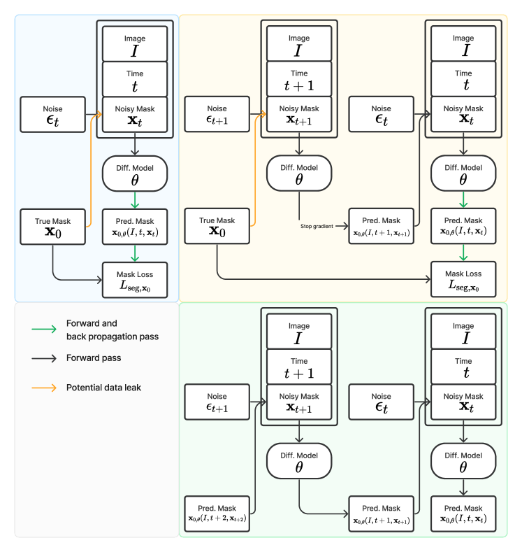
Figure 1: Illustration of training with and without recycling and inference, using mask prediction. For training without recycling (top left), the noisy mask $\mathbf{x}_{t}$ is calculated using the ground truth mask. For training with recycling (top right), $\mathbf{x}_{t}$ is calculated using prediction from the previous step, which is similar to the inference (bottom right).

3.1 DDPM for Segmentation

The denoising diffusion probabilistic models (DDPM) (Sohl-Dickstein et al., 2015; Ho et al., 2020; Nichol and Dhariwal, 2021; Kingma et al., 2021) consider a forward process: given sample $\mathbf{x}_{0}\sim q(\mathbf{x}_{0})$, noisy $\mathbf{x}_{t}$ for $t=1,\cdots,T$ follows a multivariate normal distribution, $q(\mathbf{x}_{t}\mid\mathbf{x}_{t-1})=\mathcal{N}(\mathbf{x}_{t};\sqrt{1-\beta_{t}}\mathbf{x}_{t-1},\beta_{t}\mathbf{I})$, where $\beta_{t}\in[0,1]$. Given a sufficiently large $T$, $\mathbf{x}_{T}$ approximately follows an isotropic multivariate normal distribution $\mathcal{N}(\mathbf{x}_{T};\mathbf{0},\mathbf{I})$. A reverse process is then defined to denoise $\mathbf{x}_{t}$ at each step, for $t=T,\cdots,1$, $p_{\theta}(\mathbf{x}_{t-1}\mid\mathbf{x}_{t})=\mathcal{N}(\mathbf{x}_{t-1};\bm{\mu}_{\theta}(\mathbf{x}_{t},t),\tilde{\beta}_{t}\mathbf{I})$, with a predicted mean $\bm{\mu}_{\theta}(\mathbf{x}_{t},t)$ and a variance schedule $\tilde{\beta}_{t}\mathbf{I}$. $\tilde{\beta}_{t}=\frac{1-\bar{\alpha}_{t-1}}{1-\bar{\alpha}_{t}}\beta_{t}$, where $\alpha_{t}=1-\beta_{t}$, $\bar{\alpha}_{t}=\prod_{s=0}^{t}\alpha_{s}$. $\bm{\mu}_{\theta}(\mathbf{x}_{t},t)$ can be modelled in two different ways,

$$\bm{\mu}_{\theta}(\mathbf{x}_{t},t) =\frac{\sqrt{\bar{\alpha}_{t-1}}\beta_{t}}{1-\bar{\alpha}_{t}}\mathbf{x}_{0,\theta}(\mathbf{x}_{t},t)+\frac{1-\bar{\alpha}_{t-1}}{1-\bar{\alpha}_{t}}\sqrt{\alpha_{t}}\mathbf{x}_{t},\leavevmode\nobreak\ (\text{Predict}\leavevmode\nobreak\ \mathbf{x}_{0})$$ (1)

$$\bm{\mu}_{\theta}(\mathbf{x}_{t},t) =\frac{1}{\sqrt{\alpha}_{t}}(\mathbf{x}_{t}-\frac{\beta_{t}}{\sqrt{1-\bar{\alpha}_{t}}}\bm{\epsilon}_{t,\theta}(\mathbf{x}_{t},t)),\leavevmode\nobreak\ (\text{Predict noise}\leavevmode\nobreak\ \bm{\epsilon}_{t})$$ (2)

where $\mathbf{x}_{0,\theta}(\mathbf{x}_{t},t)$ or $\bm{\epsilon}_{t,\theta}(\mathbf{x}_{t},t)$ are the learned neural network.

For segmentation, $\mathbf{x}$ represents a transformed probability with values in $[-1,1]$. Particularly, $\mathbf{x}_{0}\in\{1,-1\}$ are binary-valued, transformed from mask. $\mathbf{x}_{0,\theta}$ and $\mathbf{x}_{t}$ ($t\geq 0$) have values in $[-1,1]$. Moreover, the networks $\mathbf{x}_{0,\theta}(I,\mathbf{x}_{t},t)$ or $\bm{\epsilon}_{t,\theta}(I,\mathbf{x}_{t},t)$ takes one more input $I$, representing the image to segment.

3.2 Recycling

During training, existing methods samples $\mathbf{x}_{t}$ by interpolating noise $\bm{\epsilon}_{t}$ and ground-truth $\mathbf{x}_{0}$, which results in a certain level of data leak (Chen et al., 2022; Young et al., 2022). Kolbeinsson and Mikolajczyk (2022) proposed recursive denoising, which performed $T$ steps on each image progressively to use model’s predictions at previous steps. However, this extends the training length $T$ times. Instead, in this work, for each image, the time step $t$ is randomly sampled and the model’s prediction $\mathbf{x}_{0,\theta}$ from the previous time step $t+1$ is recycled to replace ground-truth (Fig. 1).

Similar reuses of the model’s predictions have been previously applied in 2D image segmentation (Chen et al., 2022), however $\mathbf{x}_{0,\theta}$ was fed into the network along with $\mathbf{x}_{t}$ which requires additional memories and still has data leak risks. A further difference to these previous approaches is that, rather than stochastic recycling, usually with a probability of $50\%$, it is always applied throughout the training (which was empirically found to lead to more stable and performant model training). Formally, the recycling technique at a sampled step $t$ is as follows,

$$\mathbf{x}_{t+1} =\sqrt{\bar{\alpha}_{t+1}}\mathbf{x}_{0}+\sqrt{1-\bar{\alpha}_{t+1}}\bm{\epsilon}_{t+1},\leavevmode\nobreak\ \text{(Noise mask generation for}\leavevmode\nobreak\ t+1)$$ (3)

$$\mathbf{x}_{0,\theta} =\text{StopGradient}(\mathbf{x}_{0,\theta}(I,t+1,\mathbf{x}_{t+1})),\leavevmode\nobreak\ \text{(Mask prediction)}$$ (4)

$$\mathbf{x}_{t} =\sqrt{\bar{\alpha}_{t}}\mathbf{x}_{0,\theta}+\sqrt{1-\bar{\alpha}_{t}}\bm{\epsilon}_{t},\leavevmode\nobreak\ \text{(Noise mask generation for}\leavevmode\nobreak\ t)$$ (5)

where $\mathbf{x}_{0,\theta}$ is the predicted segmentation mask from $t+1$ using ground-truth, with gradient stopping. $\bm{\epsilon}_{t}$ and $\bm{\epsilon}_{t+1}$ are two independently sampled noises. Recycling can be applied to models predicting noise (see supplementary materials Section 1 for derivation and illustration).

3.3 Loss

Given noised mask $\mathbf{x}_{t}$, time $t$, and image $I$, the loss can be,

$$L_{\text{seg},\mathbf{x}_{0}}(\theta) =\mathbb{E}_{t,\mathbf{x}_{0},\bm{\epsilon}_{t},I}\mathcal{L}_{\text{seg}}(\mathbf{x}_{0},\leavevmode\nobreak\ \mathbf{x}_{0,\theta}),$$ (6)

$$L_{\text{seg},\bm{\epsilon}_{t}}(\theta) =\mathbb{E}_{t,\mathbf{x}_{0},\bm{\epsilon}_{t},I}\|\bm{\epsilon}_{t}-\bm{\epsilon}_{t,\theta}\|_{2}^{2},$$ (7)

where model predict noise $\bm{\epsilon}_{t,\theta}$ or mask $\mathbf{x}_{0,\theta}$ and $\mathcal{L}_{\text{seg}}$ represents a segmentation-specific loss, such as Dice loss or cross-entropy loss. $t$ is sampled from $1$ to $T$, $\bm{\epsilon}_{t}\sim\mathcal{N}(\mathbf{0},\mathbf{I})$, and $\mathbf{x}_{t}(\mathbf{x}_{0},\bm{\epsilon}_{t})=\sqrt{\bar{\alpha}_{t}}\mathbf{x}_{0}+\sqrt{1-\bar{\alpha}_{t}}\bm{\epsilon}_{t}$. When model predicts noise, segmentation loss can still be used as the mask can be inferred via interpolation.

3.4 Variance resampling

During training or inference, given a variance schedule $\{\beta_{t}\}_{t=1}^{T}$ for $T=1000$, a subsequence $\{\beta_{k}\}_{k=1}^{K}$ for $K=5$ can be sampled with $\{t_{k}\}_{k=1}^{K}$, where $t_{K}=T$, $t_{1}=1$,$\beta_{k}=1-\frac{\bar{\alpha}_{t_{k}}}{\bar{\alpha}_{t_{k-1}}},\tilde{\beta}_{k}=\frac{1-\bar{\alpha}_{t_{k}-1}}{1-\bar{\alpha}_{t_{k}}}\beta_{t_{k}}$. $\alpha_{k}$ and $\bar{\alpha}_{k}$ are recalculated correspondingly.

4 Experiment Setting

Prostate MR The data set (Li et al., 2022) contains $589$ T2-weighted image-mask pairs for $8$ anatomical structures. The images were randomly split into non-overlapping training, validation, and test sets, with $411$, $14$, $164$ images in each split, respectively. All images were normalised, resampled, and centre-cropped to an image size of $256\times 256\times 48$, with a voxel dimension of $0.75\times 0.75\times 2.5$ (mm).
Abdominal CT The data set (Ji et al., 2022) provides $200$ and $100$ CT image-mask pairs for $15$ abdominal organs in training and validation sets. The validation set was randomly split into non-overlapping validation and test sets, with $10$ and $90$ images, respectively. HU values were clipped to $[-991,362]$ for all images. Images were then normalised, resampled and centre-cropped to an image size of $192\times 128\times 128$, with a voxel dimension of $1.5\times 1.5\times 5.0$ (mm).
Implementation  3D U-nets have four layers with $32$, $64$, $128$, and $256$ channels. For diffusion models, noise-corrupted masks and images were concatenated along feature channels and time was encoded using sinusoidal positional embedding (Rombach et al., 2022). Random rotation, translation and scaling were adopted for data augmentation during training. The segmentation-specific loss function is by default the sum of cross-entropy and foreground-only Dice loss. When predicting noise, the $L_{2}$ loss has a weight of $0.1$ (Wu et al., 2022). All models were trained with AdamW for $12500$ steps and a warmup cosine learning rate schedule. Hyper-parameter were configured empirically without extensive tuning. Binary Dice score and $95\%$ Hausdorff distance in mm (HD), averaged over foreground classes, were reported. Paired Student’s t-tests were performed on Dice score to test statistical significance between model performance with $\alpha=0.01$. Experiments were performed using bfloat16 mixed precision on TPU v3-8. The code is available at https://github.com/mathpluscode/ImgX-DiffSeg.

5 Results

Recycling The performance of the proposed diffusion model is summarised in Table 1. With recycling, the diffusion-based 3D models reached a Dice score of $0.830$ and $0.801$ which is statistically significantly ($p<0.001$) higher than baseline diffusion with $0.815$ and $0.753$, for prostate MR and abdominal CT respectively. Example predictions were provided in Fig. 2.
Diffusion vs Non-diffusion  The diffusion model is also compared with U-net trained via standard supervised learning in Table 2. Within the same computing budget, the diffusion-based 3D model is competitive with its non-diffusion counterpart. The results in Fig. 2 are also visually comparable. The difference, however, remains significant with $p<0.001$.
Ablation studies  Comparisons were performed on prostate MR data set for other modifications, including: 1) predicting mask instead of noise 2) using Dice loss in addition to cross-entropy, 3) using five steps denoising process during training. Improvements in Dice score between $0.09$ and $0.117$ were observed for all modifications (all p-values $<0.001$). The largest improvement was observed when the model predicted segmentation masks instead of noise. The results were found consistent with the consistency model (Song et al., 2023), which requests diffusion models’ predictions of $\mathbf{x}_{0}$ from different time steps to be similar. Such requirement is implicitly met in our applications as the segmentation loss requires the prediction to be consistent with the ground truth mask given an image. As a result, the predictions from different time steps shall be consistent.
Limitation In general, all methods tend to perform better for large regions of interest (ROI), and there is a significant correlation (Spearman $r>0.8$ and $p<0.01$) between ROI (regions of interest) area and mean Dice score per ROI/class, indicating room of future improvement by addressing small ROIs.

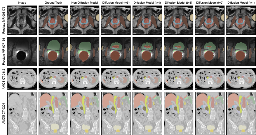
Figure 2: Example predictions from diffusion and non-diffusion U-net models.

Table 1: DDPM with recycling.

Recycling	Prostate MR		Abdominal CT
	Dice Score	Hausdorff Dist.	Dice Score	Hausdorff Dist.
N	$0.815\pm 0.095$	$5.485\pm 1.069$	$0.753\pm 0.131$	$9.526\pm 2.232$
Y	$0.830\pm 0.094$	$5.424\pm 1.176$	$0.801\pm 0.109$	$9.125\pm 2.564$

Table 2: Comparison between diffusion models and non-diffusion models.

Diffusion	Prostate MR		Abdominal CT
	Dice score	Hausdorff Dist.	Dice score	Hausdorff Dist.
N	$0.838\pm 0.088$	$5.197\pm 1.184$	$0.816\pm 0.100$	$9.091\pm 2.475$
Y	$0.830\pm 0.094$	$5.424\pm 1.176$	$0.801\pm 0.109$	$9.125\pm 2.564$

Table 3: Ablation results (prostate MR). HD stands for Hausdorff distance.

Output	Dice Score	HD
Noise	0.713	23.855
Logits	0.830	5.424

(a)

Dice Loss	Dice Score	HD
N	0.812	5.463
Y	0.830	5.424

(b)

Steps	Dice Score	HD
1000	0.821	5.223
5	0.830	5.424

(c)

6 Discussion

In this work, we developed a novel denoising diffusion probabilistic model for 3D image multiclass segmentation. By recycling the model’s predictions at previous time steps to replace ground truth during training, the method aligns diffusion training and segmentation evaluation, resulting in significant performance improvements compared to existing diffusion methods. Other techniques mitigating training and test inconsistency further improved the diffusion model’s performance. However, the diffusion model did not outperform the non-diffusion-based segmentation models, which have long been well-established. We believe it is important to report this lack of superior performance in 3D medical image segmentation, especially when experiments are limited to the same compute budget. Future work could consider other diffusion models such as discrete diffusion and more memory-efficient implementation to enable more complex architectures. Although the presented experimental results primarily demonstrated methodological development, the fact that these were obtained on two large clinical data sets represents a promising step towards real-world applications. Localising multiple anatomical structures in prostate MR images is key to MR-targeted biopsy, radiotherapy and tissue-preserving focal treatment for patients with urological diseases, while abdominal organ outlines can be directly used in planning gastroenterological procedures and hepatic surgery.

7 Acknowledgement

This work was supported by the EPSRC grant (EP/T029404/1), the Wellcome/EPSRC Centre for Interventional and Surgical Sciences (203145Z/16/Z), the International Alliance for Cancer Early Detection, an alliance between Cancer Research UK (C28070/A30912, C73666/A31378), Canary Center at Stanford University, the University of Cambridge, OHSU Knight Cancer Institute, University College London and the University of Manchester, and Cloud TPUs from Google’s TPU Research Cloud (TRC).

Appendix

Recycling can be applied to models predicting noise as below (Figure 3),

$$\mathbf{x}_{t+1} =\sqrt{\bar{\alpha}_{t+1}}\mathbf{x}_{0}+\sqrt{1-\bar{\alpha}_{t+1}}\bm{\epsilon}_{t+1},\leavevmode\nobreak\ \text{(Noise mask generation for}\leavevmode\nobreak\ t+1)$$ (8)

$$\bm{\epsilon}_{t+1,\theta} =\text{StopGradient}(\bm{\epsilon}_{t+1,\theta}(I,t+1,\mathbf{x}_{t+1})),\leavevmode\nobreak\ \text{(Noise prediction)}$$ (9)

$$\mathbf{x}_{0,\theta} =\frac{1}{\sqrt{\bar{\alpha}_{t+1}}}(\mathbf{x}_{t+1}-\sqrt{1-\bar{\alpha}_{t+1}}\bm{\epsilon}_{t+1,\theta}),\leavevmode\nobreak\ \text{(Mask prediction)}$$ (10)

$$\mathbf{x}_{t} =\sqrt{\bar{\alpha}_{t}}\mathbf{x}_{0,\theta}+\sqrt{1-\bar{\alpha}_{t}}\bm{\epsilon}_{t}.\leavevmode\nobreak\ \text{(Noise mask generation for}\leavevmode\nobreak\ t)$$ (11)

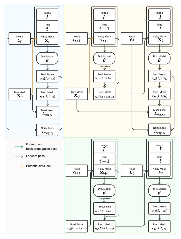
Figure 3: Illustration of training with and without recycling, and inference, using noise prediction. For training without recycling (top left), the noisy mask $\mathbf{x}_{t}$ is calculated using the ground truth mask. For training with recycling (top right), $\mathbf{x}_{t}$ is calculated using prediction from the previous step, which is similar to the inference (bottom right).

References

- Li et al. [2021] Xiaoxiao Li, Yuan Zhou, Nicha Dvornek, Muhan Zhang, Siyuan Gao, Juntang Zhuang, Dustin Scheinost, Lawrence H Staib, Pamela Ventola, and James S Duncan. Braingnn: Interpretable brain graph neural network for fmri analysis. Medical Image Analysis, 74:102233, 2021.
- Strudel et al. [2021] Robin Strudel, Ricardo Garcia, Ivan Laptev, and Cordelia Schmid. Segmenter: Transformer for semantic segmentation. In Proceedings of the IEEE/CVF international conference on computer vision, pages 7262–7272, 2021.
- Fu et al. [2019] Yunguan Fu, Maria R Robu, Bongjin Koo, Crispin Schneider, Stijn van Laarhoven, Danail Stoyanov, Brian Davidson, Matthew J Clarkson, and Yipeng Hu. More unlabelled data or label more data? a study on semi-supervised laparoscopic image segmentation. arXiv preprint arXiv:1908.08035, 2019.
- Li et al. [2022] Yiwen Li, Yunguan Fu, Iani Gayo, Qianye Yang, Zhe Min, Shaheer Saeed, Wen Yan, Yipei Wang, J Alison Noble, Mark Emberton, et al. Prototypical few-shot segmentation for cross-institution male pelvic structures with spatial registration. arXiv preprint arXiv:2209.05160, 2022.
- Ronneberger et al. [2015] Olaf Ronneberger, Philipp Fischer, and Thomas Brox. U-net: Convolutional networks for biomedical image segmentation. In Medical Image Computing and Computer-Assisted Intervention–MICCAI 2015: 18th International Conference, Munich, Germany, October 5-9, 2015, Proceedings, Part III 18, pages 234–241. Springer, 2015.
- Ji et al. [2022] Yuanfeng Ji, Haotian Bai, Jie Yang, Chongjian Ge, Ye Zhu, Ruimao Zhang, Zhen Li, Lingyan Zhang, Wanling Ma, Xiang Wan, et al. Amos: A large-scale abdominal multi-organ benchmark for versatile medical image segmentation. arXiv preprint arXiv:2206.08023, 2022.
- Ho et al. [2020] Jonathan Ho, Ajay Jain, and Pieter Abbeel. Denoising diffusion probabilistic models. Advances in Neural Information Processing Systems, 33:6840–6851, 2020.
- Dhariwal and Nichol [2021] Prafulla Dhariwal and Alexander Nichol. Diffusion models beat gans on image synthesis. Advances in Neural Information Processing Systems, 34:8780–8794, 2021.
- Ho and Salimans [2022] Jonathan Ho and Tim Salimans. Classifier-free diffusion guidance. arXiv preprint arXiv:2207.12598, 2022.
- Amit et al. [2021] Tomer Amit, Eliya Nachmani, Tal Shaharbany, and Lior Wolf. Segdiff: Image segmentation with diffusion probabilistic models. arXiv preprint arXiv:2112.00390, 2021.
- Kolbeinsson and Mikolajczyk [2022] Benedikt Kolbeinsson and Krystian Mikolajczyk. Multi-class segmentation from aerial views using recursive noise diffusion. arXiv preprint arXiv:2212.00787, 2022.
- Wolleb et al. [2022] Julia Wolleb, Robin Sandkühler, Florentin Bieder, Philippe Valmaggia, and Philippe C Cattin. Diffusion models for implicit image segmentation ensembles. In International Conference on Medical Imaging with Deep Learning, pages 1336–1348. PMLR, 2022.
- Wu et al. [2022] Junde Wu, Huihui Fang, Yu Zhang, Yehui Yang, and Yanwu Xu. Medsegdiff: Medical image segmentation with diffusion probabilistic model. arXiv preprint arXiv:2211.00611, 2022.
- Chen et al. [2022] Ting Chen, Lala Li, Saurabh Saxena, Geoffrey Hinton, and David J Fleet. A generalist framework for panoptic segmentation of images and videos. arXiv preprint arXiv:2210.06366, 2022.
- Young et al. [2022] Sean I Young, Adrian V Dalca, Enzo Ferrante, Polina Golland, Bruce Fischl, and Juan Eugenio Iglesias. Sud: Supervision by denoising for medical image segmentation. arXiv preprint arXiv:2202.02952, 2022.
- Lai et al. [2023] Zeqiang Lai, Yuchen Duan, Jifeng Dai, Ziheng Li, Ying Fu, Hongsheng Li, Yu Qiao, and Wenhai Wang. Denoising diffusion semantic segmentation with mask prior modeling. arXiv preprint arXiv:2306.01721, 2023.
- Nichol and Dhariwal [2021] Alexander Quinn Nichol and Prafulla Dhariwal. Improved denoising diffusion probabilistic models. In International Conference on Machine Learning, pages 8162–8171. PMLR, 2021.
- Sohl-Dickstein et al. [2015] Jascha Sohl-Dickstein, Eric Weiss, Niru Maheswaranathan, and Surya Ganguli. Deep unsupervised learning using nonequilibrium thermodynamics. In International Conference on Machine Learning, pages 2256–2265. PMLR, 2015.
- Radford et al. [2021] Alec Radford, Jong Wook Kim, Chris Hallacy, Aditya Ramesh, Gabriel Goh, Sandhini Agarwal, Girish Sastry, Amanda Askell, Pamela Mishkin, Jack Clark, et al. Learning transferable visual models from natural language supervision. In International conference on machine learning, pages 8748–8763. PMLR, 2021.
- Ali et al. [2023] Hazrat Ali, Shafaq Murad, and Zubair Shah. Spot the fake lungs: Generating synthetic medical images using neural diffusion models. In Artificial Intelligence and Cognitive Science: 30th Irish Conference, AICS 2022, Munster, Ireland, December 8–9, 2022, Revised Selected Papers, pages 32–39. Springer, 2023.
- Pinaya et al. [2022] Walter HL Pinaya, Petru-Daniel Tudosiu, Jessica Dafflon, Pedro F da Costa, Virginia Fernandez, Parashkev Nachev, Sebastien Ourselin, and M Jorge Cardoso. Brain imaging generation with latent diffusion models. arXiv preprint arXiv:2209.07162, 2022.
- Kim and Ye [2022] Boah Kim and Jong Chul Ye. Diffusion deformable model for 4d temporal medical image generation. In Medical Image Computing and Computer Assisted Intervention–MICCAI 2022: 25th International Conference, Singapore, September 18–22, 2022, Proceedings, Part I, pages 539–548. Springer, 2022.
- Saeed et al. [2023] Shaheer U. Saeed, Tom Syer, Wen Yan, Qianye Yang, Mark Emberton, Shonit Punwani, Matthew J. Clarkson, Dean C. Barratt, and Yipeng Hu. Bi-parametric prostate mr image synthesis using pathology and sequence-conditioned stable diffusion. arXiv preprint arXiv:2303.02094, 2023.
- Khader et al. [2022] Firas Khader, Gustav Mueller-Franzes, Soroosh Tayebi Arasteh, Tianyu Han, Christoph Haarburger, Maximilian Schulze-Hagen, Philipp Schad, Sandy Engelhardt, Bettina Baessler, Sebastian Foersch, et al. Medical diffusion–denoising diffusion probabilistic models for 3d medical image generation. arXiv preprint arXiv:2211.03364, 2022.
- Baranchuk et al. [2021] Dmitry Baranchuk, Ivan Rubachev, Andrey Voynov, Valentin Khrulkov, and Artem Babenko. Label-efficient semantic segmentation with diffusion models. arXiv preprint arXiv:2112.03126, 2021.
- Kingma et al. [2021] Diederik Kingma, Tim Salimans, Ben Poole, and Jonathan Ho. Variational diffusion models. Advances in neural information processing systems, 34:21696–21707, 2021.
- Rombach et al. [2022] Robin Rombach, Andreas Blattmann, Dominik Lorenz, Patrick Esser, and Björn Ommer. High-resolution image synthesis with latent diffusion models. In Proceedings of the IEEE/CVF Conference on Computer Vision and Pattern Recognition, pages 10684–10695, 2022.
- Song et al. [2023] Yang Song, Prafulla Dhariwal, Mark Chen, and Ilya Sutskever. Consistency models. arXiv preprint arXiv:2303.01469, 2023.