What do surveys say about the historical trend of inequality and the applicability of two table-transformation methods?

Abstract: We apply a pseudo panel analysis of survey data from the years 2010 and 2017 about Americans’ self-reported marital preferences and perform some formal tests on the sign and magnitude of the change in educational homophily from the generation of the early Boomers to the late Boomers, as well as from the early GenerationX to the late GenerationX. In the analysis, we control for changes in preferences over the course of the survey respondents’ lives. We use the test results to decide whether the popular iterative proportional fitting (IPF) algorithm, or its alternative, the NM-method is more suitable for analyzing revealed marital preferences. These two methods construct different tables representing counterfactual joint educational distributions of couples. Thereby, they disagree on the trend of revealed preferences identified from the prevalence of homogamy by counterfactual decompositions. By finding self-reported homophily to display a U-shaped pattern, our tests reject the hypothesis that the IPF is suitable for constructing counterfactuals in general, while we cannot reject the applicability of the NM. The significance of our survey-based method-selection is due to the fact that the choice between the IPF and the NM makes a difference not only to the identified historical trend of revealed homophily, but also to what future paths of social inequality are believed to be possible.

1 Introduction

In the assortative mating literature, it is a traditional approach to identify social trends by analyzing changes in the joint distributions of couples from one generation to another generation. The joint distributions reflect revealed marital/ mating preferences at the aggregate level and thereby are informative about which groups are considered to be in fit socially in each of the generations studied (see Lichter and Qian 2019).

As it is shown in the literature and also discussed in this paper, the trend of revealed homophily is sensitive to the choice of the method used for its identification. Therefore, it is insightful to compare these trends with the trend of self-reported marital preferences. In this paper, we perform a pseudo panel analysis of survey data from two waves on Americans’ self-reported preferences and test some hypotheses on the trend of homophily. These tests facilitate the choice of the method to be used for analyzing revealed preferences.

As to the revealed preferences, the challenge of identification is due to the fact that the observed matching outcome depends not only on the marital homophily (or, aggregate marital preferences, or, marital social norms, or, social barriers to marry out of ones’ group, or, social gap between different groups, or, segmentation of the marriage market, or, degree of sorting), but also on the structural availability of prospective partners with different traits (see e.g. Kalmijn 1998). Therefore, researchers aiming at documenting changes in the social divides with marriage data have to net the effect of changing aggregate preferences from that of the changing structural availability.

For instance, if the assorted trait studied is the education level then changes in the social gap among different education groups can be identified from the changes in the share of educationally homogamous couples by controlling for the effects of changing education levels of marriageable men and women.

Constructing counterfactuals is the key step of such decompositions since the following two questions cannot be answered without them. First, what would be the share of educationally homogamous couples in a certain generation provided women and men in this generation had the same education levels as their peers used to have in an earlier generation. Second, what would be the share of educationally homogamous couples in a certain generation provided this generation had the same aggregate marital preferences for spousal education as an earlier generation used to have in the past.

Up to now, the most popular method for constructing counterfactual joint distributions in the form of counterfactual contingency tables was the table-transformation method called the iterative proportional fitting algorithm (hereafter IPF algorithm). The IPF algorithm is a scaling procedure which standardizes the marginal distributions of a contingency table to a fixed value (where the marginal distributions represent the structural availability), while retaining a specific association between the row and the column variables. Its preserved association is captured by the odds-ratio.

As it is put by Aristotle, “it is impossible, or not easy, to alter by argument what has long been absorbed by habit.” Despite of Aristotle’s claim, we dare to argue that the habit of many researchers to construct counterfactuals with the IPF has a better alternative.

In this paper, we compare the IPF with the table-transformation method recently proposed by Naszodi and Mendonca (2019) and Naszodi and Mendonca (2021a) (henceforth NM-method). The transformed table obtained with the NM has the same preset marginal distributions as the transformed table obtained with the IPF. However, the NM-transformation is invariant to the ordinal indicator proposed by Liu and Lu (2006) (henceforth, LL-indicator), rather than being invariant to the cardinal odds-ratio.

The focus of this paper is on the empirical performances of the IPF-based and NM-based counterfactual decompositions at quantifying the dynamics of that dimension of inequality, which is in the center of interest of the educational assortative mating literature. This dimension of inequality is considered to increase (decrease) between different education groups if the aggregate preferences for educational homogamy or well-educated partners are found to be stronger (weaker) in a later generation relative to an earlier generation.

As to the empirical results, Naszodi and Mendonca (2021a) (as well as Naszodi 2023) get qualitatively different findings by applying the IPF and the NM for counterfactual decompositions using US census data. In particular, by studying the revealed preferences of young American adults with the IPF, the American late Boomers are found to be more “picky” about spousal education than the early Boomers. By contrast, the NM supports the opposite result.

Regarding the quantitative results, the IPF suggests that the share of educationally homogamous young couples would have increased by one percentage point (pp) if only the marital preferences had changed from the generation of the early Boomers to the generation of the late Boomers. By contrast, the NM quantifies the same ceteris paribus effect to have the opposite sign as being minus three pp (see the dark bars in Figure 1 for the period 1980–1990).

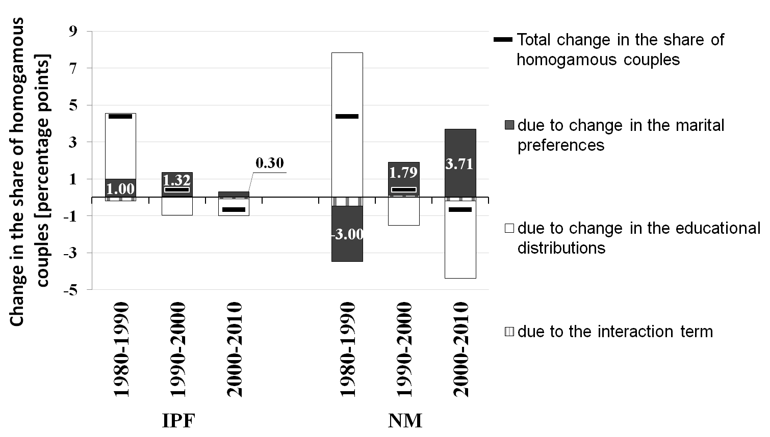
Figure 1: Decomposition of changes in the share of educationally homogamous couples between 1980 and 2010 in the US – male partners are 30–35 years old

Notes: Partial replication of Figure 1b in Naszodi and Mendonca (2021a). They use census data from IPUMS about both the education level of married couples and cohabiting couples in 1980, 1990, 2000 and 2010. The male partners aged 30–35 years in 1980, 1990, 2000 and 2010 belong to the generations of the early Boomers, the late Boomers, the early GenerationX and the late GenerationX, respectively. The educational attainment can take three different values: “Low”: no high school degree, “Medium”: high school degree without tertiary level diploma, and “High”: tertiary level diploma. Accordingly, the educationally homogamous couples are those, where both the female partner and the male partner are either “Low” educated, or both are “Medium” educated, or both are “High” educated. Changes in the prevalence of homogamy across consecutive generations are decomposed by using the so called additive decomposition scheme with interaction effects proposed by Biewen (2014), while the counterfactual tables are constructed either by the IPF, or the NM.

The two methods also disagree on whether educational homophily was much more intense in the late GenerationX than in the early GenerationX, or just slightly more intense. Quantitatively, the NM attributes almost four pp increase in the share of educationally homogamous couples to the changing homophily. Whereas the IPF quantifies the same effect to be close to zero (0.3 pp). These results can be read from the hight of the dark bars in Figure 1 corresponding to the period 2000–2010.

By exploiting the above disagreements between the methods, Naszodi and Mendonca (2021a) perform an empirical method-selection. For the selection, they present some descriptive statistics of a survey conducted by the Pew Research Center in 2010. They find that the difference between the survey responses of the early Boomers and the late Boomers, as well as the difference between the responses of the members of the early GenerationX and the late GenerationX, support the application of their method. In particular, much less late Boomers than early Boomers agreed with a statement about the importance of being well-educated by the members of the opposite sex in order to become a good spouse. And much more respondents agreed with the same statement from the late GenerationX than from the early GenerationX.

The contributions of this paper relative to the study by Naszodi and Mendonca (2021a) are three-fold. First, in this paper, we present not only some survey evidence supporting the NM in the context of assortative mating, but also some general theoretical considerations relevant for other applications as well. Second, unlike the study by Naszodi and Mendonca (2021a), this paper performs some formal hypothesis tests.

Last, but not least, we complement the preliminary survey analysis by Naszodi and Mendonca (2021a) in an important respect. Unlike Naszodi and Mendonca, we use survey data from two waves. Using a richer set of data is motivated by the following point. Although the survey data from a single wave are informative about the variations of preferences of individuals belonging to different generations, these individuals are also different in terms of their age. If the self-reported marital preferences can vary substantially over the course of individuals’ lives then the generation-effects one can identify from a single wave of a survey are not net of a potentially major confounding factor, i.e., the age-effect.

Our pseudo panel analysis of survey data from two waves allows us to identify the net generation-effects capturing what the differences between the generation-specific responses would be like if the respondents from different generations were interviewed at the same age. We study the responses of men and women survey participants separately and test the following four hypotheses:
(i) the share of “picky” men would have been lower in the population of the late Boomers than in the population of the early Boomers if every men in these two generations had been interviewed at the same age;
(ii) the share of “picky” women would have been lower in the population of the late Boomers than in the population of the early Boomers if every women in these two generations had been interviewed at the same age;
(iii) the share of “picky” men would have been much higher among the late GenerationX than among the early GenerationX if every men in these two generations had been observed at the same age;
(iv) the share of “picky” women would have been much higher among the late GenerationX than among the early GenerationX if every women in these two generations had been observed at the same age.

Depending on the results of these tests, the survey data validate either the application of the NM, or the IPF (or neither) for constructing counterfactuals.

The structure of this paper is the following. In Section 2, we present some theoretical considerations concerning the applicability of the IPF and the NM. Section 3 introduces the data and the method used for the hypothesis tests before it presents the outcome of the tests. Section 4 addresses some limitations of the tests. In Section 5, we discuss the significance of the empirical findings. Finally, Section 6 concludes the paper.

2 Some theoretical considerations concerning the applicability of the IPF and the NM

This section provides a formal definition of the table-transformation methods compared, i.e., the IPF and the NM. Also, it presents some theoretical considerations concerning their applicability.

In particular, we argue that the IPF and the NM provide solutions for two different sets of problems: while the IPF is suitable for completing a population table by using a sample from the population, the NM is fit for constructing a counterfactual population table from two population tables. Also, we make the point that the applicability of these methods for constructing counterfactuals depends on whether the association preserved by them is exactly the one we want to control for.

Finally, we illustrate with two numerical examples that the transformed tables obtained with the IPF can be sensitive to the choice of the number of trait categories. Thereby, the outcomes of certain counterfactual decompositions are also sensitive to the same choice provided the counterfactual tables are constructed by the IPF rather than the NM.

Suppose that there are two contingency tables, denoted by $P$ and $Q$, of the same size representing joint distributions of two categorical traits. E.g., $P$ and $Q$ can represent the joint distribution of husbands’ and wives’ education levels in an earlier generation and a later generation, respectively. In an alternative example, $P$ represents the joint distribution of objects in a box by material and shape, while $Q$ represents the joint distribution of objects in a random sample taken from the box.

The IPF algorithm applied to tables $P$ and $Q$ is defined by the following two steps to be iterated until convergence. First, it factors the rows of the seed table $Q$ in order to match the row totals of $P$. The table obtained after the first step (to be denoted by $Q^{{}^{\prime}}$) may not have its column totals equal to the column totals of $P$. In this case, it is necessary to perform a second step. As the second step, the IPF factors the columns of $Q^{{}^{\prime}}$ to match the corresponding column totals of $P$. The table obtained after this step (to be denoted by $Q^{{}^{\prime\prime}}$) may not have its row totals equal to the row totals of $P$. In this case, repeating the first step is necessary with $Q=Q^{{}^{\prime\prime}}$. Alternatively, we stop the iteration.

The table constructed by the IPF is the last value of $Q^{{}^{\prime\prime}}$. Let us visit some of its properties. Table $Q^{{}^{\prime\prime}}$ has row totals that match the row totals of $P$, also its column totals match the column totals of $P$ by construction. More importantly, it has the same odds-ratio as table $Q$ provided $Q$ and $P$ are 2-by-2 tables, because the odds-ratio is retained in each step of the algorithm.

The IPF was invented by Stephan and Deming (1940). It is important to note that they developed the IPF with a purpose different from constructing counterfactuals. Their purpose was to estimate a contingency table of a population from its known marginal distributions and a known contingency table of a random sample from the same population. In this exercise of “completing a population table by using a sample”, both the marginal distributions and the sample characterize the same population (e.g. the population of objects in a box); moreover, the marginal distributions and the sample are observed in the same time period.

Our first theoretical point related to the applicability of the IPF is this. The set of problems of “completing a population table” is different from the set of problems of “constructing a counterfactual table”. In contrast to the problems of “completing a population table”, in the exercises of “constructing a counterfactual table”, the marginal distributions and the seed table characterize two different populations (e.g., the populations of two generations). Accordingly, the table constructed represents a counterfactual prediction. For instance, in the context of assortative mating, it can represent a prediction on what the marriage patterns would be like in a generation if only the preferences had changed relative to an earlier generation, but not the structural availability.

Our second point is about the equivalence of the IPF and the maximum likelihood estimator and their applicability. In the “completing a population table” exercise, the maximum likelihood estimator is a natural candidate for estimating the missing values in the population table by using data in a random sample. However, nothing justifies the application of the maximum likelihood for estimating a population table from two population tables. So, nothing justifies the application of the maximum likelihood for constructing a counterfactual prediction from the observations of two populations. Actually, the IPF constructs the same table as the maximum likelihood estimator (see Meyer 1980). Therefore, there is no guarantee that the IPF would fit for estimating counterfactual tables either, even if it is perfectly suitable for the purpose it was originally developed for.

Our third theoretical point is this. Using the IPF to construct a counterfactual prediction in the context of assortative mating implicitly assumes that the aggregate marital preferences, or the degree of sorting in the two generations are characterized by the kind of association the IPF preserves, while it transforms the seed table. In other contexts, the applicability of the IPF relies on the same kind of assumption as the one in the context of assortative mating: the association preserved is assumed to be exactly the one we want to control for. Stephan and Deming recognized the crucial role of this assumption. They even warned that their algorithm is “not by itself useful for prediction” (see Stephan and Deming 1940 p.444).

Finally, we present two numerical examples for the application of the IPF with ordered assorted traits. These examples illustrate the point that the transformed tables obtained with the IPF can be sensitive to the choice of the trait categories. More precisely, the IPF does not commute with the operations of merging neighboring categories of the assorted traits. Such a sensitivity can be especially problematic if the ordered trait variables (e.g. the husbands’ and the wives’ education levels) are available at a relatively high granularity. It allows the researcher to manipulate the result of the counterfactual decompositions performed with the IPF, even unconsciously.

In our first numerical example, the assorted traits are dichotomous (e.g., both the husbands’ and the wives’ education level can take the values $L$ and $H$). Accordingly, $P$ and $Q$ are 2-by-2 contingency tables: $P^{\text{num1}}=$ $\begin{bmatrix}500&700\\ 100&700\end{bmatrix}$ and $Q^{\text{num1}}=$ $\begin{bmatrix}500&500\\ 100&900\end{bmatrix}$

As a first step of the IPF algorithm, we factor the rows of the seed table $Q^{\text{num1}}$ in order to match the row totals of $P^{\text{num1}}$. The table obtained after the first step is $Q^{{}^{\prime}\text{num1}}=$ $\begin{bmatrix}600&600\\ \;80&720\end{bmatrix}$ . As a second step, we factor the columns of $Q^{{}^{\prime}\text{num1}}$ in order to match the column totals of $P^{\text{num1}}$. We get $Q^{{}^{\prime\prime}\text{num1}}=$ $\begin{bmatrix}529.41&636.36\\ \;70.59&763.64\end{bmatrix}$ . After 4 iterations, the (rounded) IPF-transformed table is $Q^{\text{IPF},\text{num1}}=$ $\begin{bmatrix}534&665\\ \;66&735\end{bmatrix}$ . In our second numerical example, one of the assorted traits is dichotomous, while the other one is trinomial (e.g. the husbands’ trait can take the values low and high, while the wives’ ordered trait can take the values low, medium and high). Tables $P$ and $Q$ are the following two 2-by-3 tables: $P^{\text{num2}}=$ $\begin{bmatrix}500&400&300\\ 100&400&300\end{bmatrix}$ and $Q^{\text{num2}}=$ $\begin{bmatrix}500&300&200\\ 100&300&600\end{bmatrix}$ . After 4 iterations, the (rounded) IPF-transformed table is $Q^{\text{IPF},\text{num2}}=$ $\begin{bmatrix}528&475&197\\ \;72&325&403\end{bmatrix}$ . By merging its last two columns, we get $Q^{\text{IPF},\text{num2},\text{merged}}=$ $\begin{bmatrix}528&672\\ \;72&728\end{bmatrix}$ . Apparently, this table is different from $Q^{\text{IPF},\text{num1}}$ despite the fact that $P^{\text{num1}}$ and $Q^{\text{num1}}$ are equal to $P^{\text{num2}}$ and $Q^{\text{num2}}$ with merged last two columns, respectively. The difference between $Q^{\text{IPF},\text{num1}}$ and $Q^{\text{IPF},\text{num2},\text{merged}}$ does not vanish if we continue iterating after the fourth step.

If the tables in the above examples represent joint educational distributions of couples in two generations, then tables $Q^{\text{IPF},\text{num1}}$ and $Q^{\text{IPF},\text{num2},\text{merged}}$ suppose to represent the joint educational distributions of couples under a counterfactual. In particular, the counterfactual is that aggregate marital preferences are the same as in the generation represented by table $Q$, while the educational distributions of marriageable men and marriageable women are the same as in the generation represented by table $P$.

The difference between $Q^{\text{IPF},\text{num1}}$ and $Q^{\text{IPF},\text{num2},\text{merged}}$ makes a difference in the outcome of a counterfactual decomposition. Out of the $\frac{500+900}{2,000}-\frac{500+700}{2,000}=10$ pp increase in the shares of educationally homogamous couples from the generation represented by table $P^{\text{num1}}$ to the generation represented by table $Q^{\text{num1}}$, we attribute either $\frac{534+735}{2,000}-\frac{500+700}{2,000}=3.45$ pp difference, or $\frac{528+728}{2,000}-\frac{500+700}{2,000}=2.8$ pp difference to the changing aggregate preferences from one generation to the other. So, the result of our decomposition is sensitive to whether we choose not to distinguish between the last two neighboring educational categories before constructing the counterfactual table with the IPF, or after it.

We make the remark that the number of categories used varies across the empirical papers in the educational assortative mating literature. For instance, Choo and Siow (2006), as well as Naszodi and Mendonca (2021a), distinguish between three educational categories (“no high school degree”, “high school graduates”, and “college graduates”). Whereas Eika, Mogstad and Zafar (2019) divide the middle category to “high school degree with no college” and “high school degree with some college”.

None of the above points rule out that the IPF can perform well in some empirical applications at constructing certain counterfactuals. However, these points show that the choice of the IPF is not sufficiently justified theoretically. Our points call for a counterfactual table constructing method that is theoretically appealing, while it can also be validated empirically.

Recently, Naszodi and Mendonca (2021a) proposed a table-transformation method, the NM-method, as an alternative to the IPF. The NM is defined as the method that transforms table $Q$ into another table with preset row sums and column sums determined by table $P$, while retaining a specific association between the row and the column variables. Its preserved association is captured by the scalar-valued LL-indicator provided $Q$ and $P$ are 2-by-2 tables. For larger tables, the retained association is captured by the matrix-valued generalized LL-measure (see Naszodi and Mendonca 2021a for the definition of the generalized LL-measure).

Let us visit an important property of the NM. It commutes with the operations of merging neighboring categories of the ordered assorted traits by construction. So, researchers applying the NM cannot directly influence the outcome of the counterfactual decompositions by choosing the granularity of the categorical variables whose joint distribution is studied. For instance, in our numerical examples, the NM-transformed table is $Q^{\text{NM,}{\text{num1}}}=Q^{\text{NM,}{\text{num2}},\text{merged}}=$ $\begin{bmatrix}520&680\\ \;80&720\end{bmatrix}$ irrespective of first merging the last two columns of $P^{\text{num2}}$ and $Q^{\text{num2}}$ before applying the NM, or the other way around.

As to the empirical validation of the NM, Naszodi and Mendonca (2021a) present some survey evidence in favor of its application in the context of analyzing changes in assortative mating by counterfactual decompositions. In the empirical part of this paper, we refine their validation exercise.

3 Data, method and the outcomes of some tests

For the analysis, we use not only the Pew Research Center’s survey called Changing American Family Survey from 2010 (that was used by Naszodi and Mendonca 2021a), but also its American Trends Panel Wave 28 Survey conducted in 2017.

In 2017, almost the same pair of questions (coded QUALHUSB and QUALWIFE) was asked as in 2010 (coded Q.23F1 and Q.24F2). The question asked from female survey participants in 2017 was: “How important, if at all, do you feel it is for a good husband or partner to be well educated?”. The question asked from male survey participants in 2017 was: “How important, if at all, do you feel it is for a good wife or partner to be well educated?”. The potential responses offered for the participants were: (i) very important; (ii) somewhat important; (iii) not too important; (iv) not at all important; (v) don’t know/ refuse to answer.

In 2010, the question Q.23F1 (Q.24F2) asked from female (/male) participants was the following. “People have different ideas about what makes a man (/woman) a good husband (/wife) or partner. For each of the qualities that I read, please tell me if you feel it is very important for a good husband (/wife) or partner to have, somewhat important, not too important, or not at all important. First, he (/she) is well educated. Is this very important for a good husband (/wife) or partner to have, somewhat important, not too important, or not at all important?” Apparently, the formulation of the questions in 2010 and 2017 were just slightly different, while the potential responses were exactly the same.

To make our results comparable with the results in Naszodi and Mendonca (2021a), we use survey data from 2010 on the same generations as they do. In particular, the early Boomers are represented in our analysis by those who were born between 1946 and 1950; the late Boomers are represented by those who were born between 1956 and 1960; the early GenerationX is represented by those who were born between 1966 and 1970; the late GenerationX is represented by those who were born between 1976 and 1980. With this choice, we sidestep the problem of determining the exact year of birth of the last members of the generations studied and that of the first members of the next generations.

Although many of the survey participants were interviewed in both of the survey waves, our survey data is not in a panel structure. In fact, the Pew Research Center shared publicly the survey data in 2017 by using broader age categories than in 2010. In particular, while the year of birth is reported in the 2010 survey data, we know only if the survey respondents in 2017 belonged to the GenerationX (i.e., belonged to the age group populated by the 37–52 years old individuals) or belonged to the Boomer generation (i.e., belonged to the 53–71 years old cohort). This variation of the age categories across the two survey waves makes it impossible to link the survey participants and to construct a panel.

Still, we can apply a pseudo panel analysis by collecting and comparing the answers given in 2010 and 2017 of those Boomers, who where born between 1946 and 1964. Also, we can compare the answers given in 2010 and 2017 by the members of the GenerationX born between 1965 and 1980. Thereby, we can quantify and control for the age-effects: how the responses of the Boomers and those of the GenerationX have changed over seven years between 2010 and 2017.

The distributions of survey participants by gender, generation and also by the dichotomous type of respondent–non-respondent are presented in the Appendix.

Our method for analyzing the survey data is the following. First, we estimate the population-shares of those men and women, who viewed spousal education to be very important. For the estimation, we apply the approximation proposed by Agresti and Coull (1998) (see Equation 6). Our estimated population-shares are not only gender-specific, but also generation-specific and period-specific since the shares vary over one generation to another and also over the survey waves. Accordingly, we denote the estimated population-shares by $\widehat{PS}_{\text{gender},\text{generation},t}$.

Second, we calculate the generation-effects with the confounding age-effects by using data from 2010 exclusively. It is calculated as the difference between the estimated population-shares in the two generations to be compared. We denote it by ${GE}_{\text{gender},\text{generations},t}$. For the late Boomers and the early Boomers, we estimate it as

$$\widehat{GE}_{\text{gender},\text{late and early Boomers},2010}=\widehat{PS}_{\text{gender},\text{late Boomers},2010}-\widehat{PS}_{\text{gender},\text{early Boomers},2010}\;.$$ (1)

Similarly, for the late GenerationX and the early GenerationX to be compared, we estimate the generation-effect by

$$\widehat{GE}_{\text{gender},\text{late and early GenX},2010}=\widehat{PS}_{\text{gender},\text{late GenX},2010}-\widehat{PS}_{\text{gender},\text{early GenX},2010}\;.$$ (2)

Third, we calculate the age-effects, i.e., how the responses of the Boomers and those in the GenerationX have changed over seven years between 2010 and 2017. Similarly to the population-shares, the age-effects are also gender-specific, generation-specific and period-specific. Accordingly, we denote it by ${AE}_{\text{gender},\text{generation},t,\Delta t}$ and estimate it as

$$\widehat{AE}_{\text{gender},\text{generation},2010,7}=\widehat{PS}_{\text{gender},\text{generation},2017}-\widehat{PS}_{\text{gender},\text{generation},2010}\;.$$ (3)

Fourth, we calculate the net generation-effects by adjusting our biased estimates on the generation-effects obtained in step two. Since the average age difference between the early Boomers and the late Boomers, as well as between the early GenerationX and the late GenerationX, is 10 years, we have to perform the adjustments with the kind of age-effects that capture how the responses of a studied generation change over 10 years. We assume that the responses of the Boomers and those in the GenerationX would have changed over ten years as much as 10/7 times the age-effects identified in step three. Accordingly, we estimate the net generation-effect for the Boomers as

$$\widehat{NGE}_{\text{gender},\text{Boomers},2010,2020}=\widehat{GE}_{\text{gender},\text{late and early Boomers},2010}+10/7\widehat{AE}_{\text{gender},\text{Boomers},2010,7}\;.$$ (4)

Whereas for the GenerationX, the net generation-effect is estimated by

$$\widehat{NGE}_{\text{gender},\text{GenX},2010,2020}=\widehat{GE}_{\text{gender},\text{late and early GenX},2010}+10/7\widehat{AE}_{\text{gender},\text{GenX},2010,7}\;.$$ (5)

Finally, we construct the confidence intervals around the point estimates. For the population-share, we rely again on the work by Agresti and Coull (1998). Following them, we assume that the distribution of the number of survey responses “very important” (denoted by $x$) out of $n$ number of total responses is binomial with the parameter $PS$. While $q=x/n$ is the sample-share of “picky” respondents, $PS$ denotes their population-share. Agresti and Coull (1998) propose to estimate the latter as

$$\widehat{PS}=(x+z^{2}/2)/(n+z^{2})\;,$$ (6)

where $z=\Phi^{-1}(1-\alpha/2)$ is the quantile of a standard normal distribution. (For example, a 95% confidence interval requires $\alpha=0.05$, thereby producing $z=1.96$.) And they propose to approximate the population-share’s symmetric confidence interval by

$$\widehat{PS}\pm z\hat{\sigma}_{PS}\;,$$ (7)

where $\hat{\sigma}_{PS}=\sqrt{\widehat{PS}(1-\widehat{PS})/(n+z^{2})}$ is the estimates for the standard error. (For the sake of simplicity, we omitted the indices of both $\widehat{PS}$ and $\hat{\sigma}_{PS}$. However, in our empirical application, both are gender-specific, generation-specific and period-specific.)

To perform the analysis, we have to set the value of a kind of correlation that we denote by $\rho$. This correlation captures to what extent the response given in 2017 by the representative survey participant resembles the response of the same person given in 2010. We calibrate $\rho$ equal to zero in our benchmark analysis, although it is not reasonable to assume the responses to be uncorrelated. As we will see, by calibrating $\rho$ to the value zero, we get maximally conservative test results. While the point estimates of $NGE$ is independent of $\rho$, its confidence interval is not.

The symmetric confidence intervals of the generation-effects, age-effects and net generation effects are calculated similarly to the confidence interval of the population-share: the upper bound and lower bound of each interval are given by the point estimates adjusted by $z$ times the estimated standard error (see Equation 7).

The standard errors of the generation-effect, the age-effect and the net generation effect are estimated by

$$\hat{\sigma}_{\text{GE},\text{gender},\text{late and early gen},t}=\sqrt{\hat{{\sigma}^{2}}_{\text{PS},\text{gender},\text{late gen},t}+\hat{{\sigma}^{2}}_{\text{PS},\text{gender},\text{early gen},t}}\;,$$ (8)

$$\hat{\sigma}_{\text{AE},\text{gender},\text{gen},t,\Delta t}=\sqrt{\hat{{\sigma}^{2}}_{\text{PS},\text{gender},\text{gen},t}+\hat{{\sigma}^{2}}_{\text{PS},\text{gender},\text{gen},t+\Delta t}-2\rho\;{\hat{\sigma}}_{\text{PS},\text{gender},\text{gen},t}{\hat{\sigma}}_{\text{PS},\text{gender},\text{gen},t+\Delta t}}\;,$$ (9)

$$\hat{\sigma}_{\text{NGE},\text{gender},\text{late and early gen},t,\Delta t}=\sqrt{\hat{{\sigma}^{2}}_{\text{GE},\text{gender},\text{late and early gen},t}+(10/7)^{2}\hat{{\sigma}^{2}}_{\text{AE},\text{gender},\text{gen},t,\Delta t}}\;,$$ (10)

respectively.

With the above notations (simplified by omitting the time indices), our hypotheses about the Boomers can be formalized as      (i) $H^{mB}_{0}:{NGE}_{\text{male},\text{Boomers}}=0$ with the alternative of either $H^{mB-}_{1}:{NGE}_{\text{male},\text{Boomers}}<0$, or $H^{mB+}_{1}:{NGE}_{\text{male},\text{Boomers}}>0$;
(ii) $H^{fB}_{0}:{NGE}_{\text{female},\text{Boomers}}=0$ with the alternative of either $H^{fB-}_{1}:{NGE}_{\text{female},\text{Boomers}}<0$, or $H^{fB+}_{1}:{NGE}_{\text{female},\text{Boomers}}>0$.

Whereas our second set of hypotheses (about the GenerationX) are
(iii) $H^{mX}_{0}:{NGE}_{\text{male},\text{GenX}}=0$ with the alternative of $H^{mX+}_{1}:{NGE}_{\text{male},\text{GenX}}>0$;
(iv) $H^{fX}_{0}:{NGE}_{\text{female},\text{GenX}}=0$ with the alternative of $H^{fX+}_{1}:{NGE}_{\text{female},\text{GenX}}>0$.

What outcomes of the tests would provide empirical support to the application of the NM and what outcomes would favor the IPF? Based on the findings of Naszodi and Mendonca (2021a) presented in Figure 1, if $H^{j}_{0}$ were rejected for all $j\in\{mB;fB;mX;fX\}$ in favor of $H^{mB-}_{1}$, $H^{fB-}_{1}$, $H^{mX+}_{1}$ and $H^{fX+}_{1}$, then our set of tests would support the NM. Similarly, if $H^{mB}_{0}$ and $H^{fB}_{0}$ were rejected in favor of $H^{mB+}_{1}$ and $H^{fB+}_{1}$, respectively, while $H^{mX}_{0}$ and $H^{fX}_{0}$ were accepted, then our tests would support the IPF.

There are some more potential outcomes that favor either the NM, or the IPF. This is because both the NM and the IPF make predictions on the changes of the equilibrium in the marriage market, rather than on its two determinants, i.e., the men’s side of the market and the women’s side of the market. The sign of the change in the share of homogamous couples under the equilibrium is the same as the sign of change in aggregate preferences at the men’s side of the market provided the preferences are unchanged at the women’s side of the market. E.g., if only men become more (/less) “picky” then the share of homogamous couples increases (/decreases). Similarly, if men’s aggregate preferences are unchanged from one generation to another, while women’s preferences change in a certain way, then the latter determines the direction of change in the equilibrium.

Accordingly, the potential outcomes of the tests that are also in favor of the NM are the following. $H^{mB}_{0}$ is rejected in favor of the alternative hypothesis of $H^{mB-}_{1}$, while $H^{fB}_{0}$ is accepted. $H^{fB}_{0}$ is rejected in favor of the alternative hypothesis of $H^{fB-}_{1}$, while $H^{mB}_{0}$ is accepted. $H^{mX}_{0}$ is rejected in favor of the alternative hypothesis of $H^{mX+}_{1}$, while $H^{fX}_{0}$ is accepted. $H^{fX}_{0}$ is rejected in favor of the alternative hypothesis of $H^{fX+}_{1}$, while $H^{mX}_{0}$ is accepted.

Similarly, we would get empirical support for the IPF in the following cases as well: $H^{mB}_{0}$ is rejected in favor of the alternative hypothesis of $H^{mB+}_{1}$, while $H^{fB}_{0}$ is accepted; $H^{fB}_{0}$ is rejected in favor of the alternative hypothesis of $H^{fB+}_{1}$, while $H^{mB}_{0}$ is accepted.

Table 1: The potential and the actual outcomes of the hypothesis tests for the Boomers

	male Boomers		$H^{mB-}_{1}:$	$H^{mB}_{0}:$	$H^{mB+}_{1}:$
			${NGE}<0$	${NGE}=0$	${NGE}>0$
			$\widehat{NGE}=-24.2pp$
			$(p_{\rho=0}=0.7\%)$
female Boomers			$(p_{\rho=1}=0.2\%)$
$H^{fB-}_{1}$: ${NGE}<0$ $\;\;\widehat{NGE}=-6.6pp$		$(p_{\rho=0}=22.0\%)$	NM	NM	neither
		$(p_{\rho=1}=18.5\%)$
$H^{fB}_{0}\;\;\;\;$: ${NGE}=0$			NM	neither	IPF
$H^{fB+}_{1}\;:{NGE}>0$			neither	IPF	IPF

Note: this table lists all the potential outcomes of the tests supporting the application of either the NM, or the IPF, or neither for constructing counterfactuals. The p-values report the actual outcomes of the tests under two extreme values of the correlation. The value $\rho=1$ ($\rho=0$) suggests that there is a perfect (no) correlation between the empirical shares of the “picky” individuals belonging to the same generation while being observed in 2010 and 2017.

Table 2: The potential and the actual outcomes of the hypothesis tests for the GenerationX

	male GenX		$H^{mX}_{0}:$	$H^{mX+}_{1}:$
			${NGE}=0$	${NGE}>0$
				$\widehat{NGE}=9.8pp$
				$(p_{\rho=0}=18.9\%)$
female GenX				$(p_{\rho=1}=16.1\%)$
$H^{fX}_{0}\;\;\;$:$\;{NGE}=0$			IPF	NM
$H^{fX+}_{1}:{NGE}>0$ $\;\;\widehat{NGE}=2.7pp$		$(p_{\rho=0}=40.0\%)$	NM	NM
		$(p_{\rho=1}=38.8\%)$

Note: same as under Table 1.

While the detailed results of our tests are presented in the Appendix, Tables 1 and 2 summarize them. Table 1 shows that at any significance level above 0.7%, our tests on the Boomers support the application of the NM, irrespective of the calibrated value of the correlation $\rho$, because the tests either accept the hypotheses $H^{mB-}_{1}$ and $H^{fB-}_{1}$ (for $\alpha/2>22\%$), or they accept the hypotheses $H^{mB-}_{1}$ and $H^{fB}_{0}$ (for $\alpha/2<18.5\%$).

Similarly to the Boomers, it is the test on the male survey respondents in the GenerationX that plays the primary role at the method-selection (see Table 2). At the 20% significance level, we can reject $H^{mX}_{0}$ and the IPF in favor of $H^{mX+}_{1}$ and the NM even under the zero correlation assumption since the related p-value is in the range of [16.1%, 18.9%].

4 Some limitations of the tests

It is generally considered that small sample surveys about self-reported preferences are inferior to population data on revealed preferences. We admit that surveys have a limited capacity for tracking precisely the trends in the center of our interest.

Accordingly, we use the survey responses exclusively to select the method suitable for analyzing revealed preferences of all individuals in the studied populations, while we do not pay much attention to the exact value of the estimated change in self-reported homophily.

Also, we admit that survey responses are potentially subject to certain biases. For instance, suppose that many survey participants share the stoical view of Epictetus that can be summarize by the following quote from him: “do not seek to have everything that happens happen as you wish, but wish for everything to happen as it actually does happen, and your life will be serene.”

The kind of estimation bias due to stoical survey respondents (who adjust their preferences to the matching outcomes ex post) does not alter our method-selection. Consider that no survey respondents were stoical among the boomers. Then fewer early boomers would have wished (or declared to prefer) to have married a well-educated partner as they actually had done. However, even much fewer late boomers would have reported to have preferred the same, because what has happened is that the prevalence of homogamy increased among the late boomers relative to the early boomers irrespective of the method used for constructing the counterfactuals (see the black tick marks in Figure 1 in the positive range corresponding to the period 1980–1990). Therefore, the decreasing effect of preferences on the prevalence of homogamy from the early Boomers to the late Boomers would be estimated to be even more sharply decreasing without the “stoical bias”.

Similarly, consider that no survey respondents were stoical in the Generation-X. Then fewer early Gen-Xers would have wished ex post to have married a well-educated partner as they actually had done. However, just slightly fewer late GenX-ers would have wished the same, because the prevalence of homogamy decreased among the late GenX-ers relative to the early GenX-ers (see the black tick marks in Figure 1 in the negative range corresponding to the period 2000–2010). So, the increasing effect of preferences on the prevalence of homogamy would be estimated to be even more sharply increasing without the “stoical bias” of the GenX-ers.

There is an additional potential issue with the survey data: in 2010 the survey respondents were approached by phone, while in 2017 the survey was conducted via web, phone and mail. However, any potential systematic bias in the generation-effect and the age-effect caused by the variation in the means of communication is controlled for by taking the difference between the share of certain responses given by consecutive generations in the same wave.

Finally, the inference on the basis of significance tests has been criticized in the statistical literature and the application of the Bayesian inference has been proposed. The Bayes factors suggest that the evidence is in favor of $H^{mB-}_{1}$, while the Bayesian tests are inconclusive about the $H^{fB}_{0}$ versus $H^{fB-}_{1}$, the $H^{mX}_{0}$ versus $H^{mX+}_{1}$ and $H^{fX}_{0}$ versus $H^{fX+}_{1}$ (see Figure 2). So, overall the Bayesian hypothesis tests also corroborate the application of the NM as a method for constructing counterfactuals.

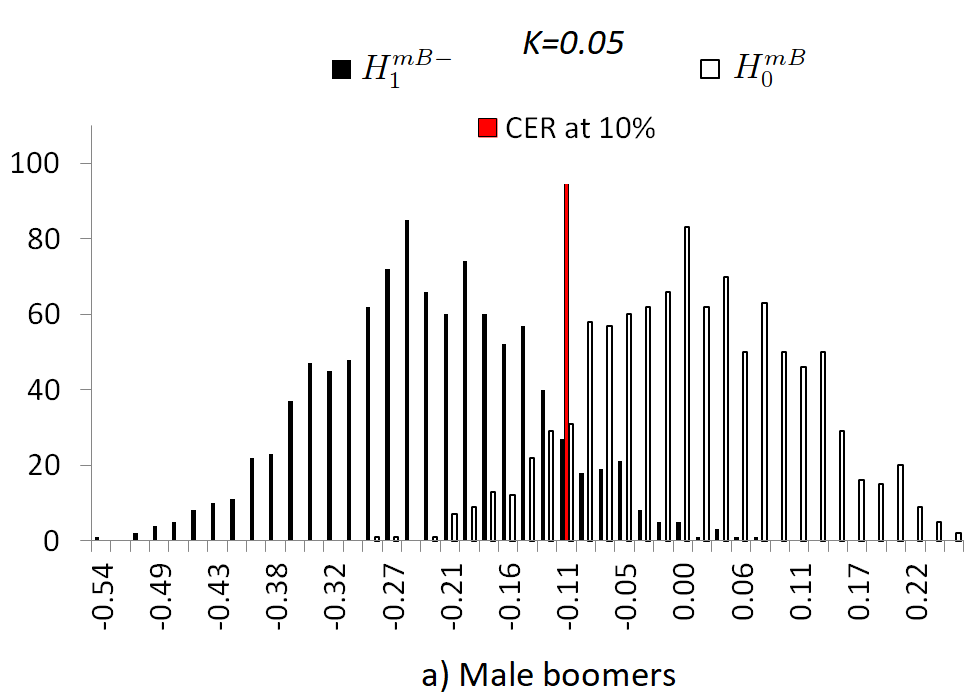
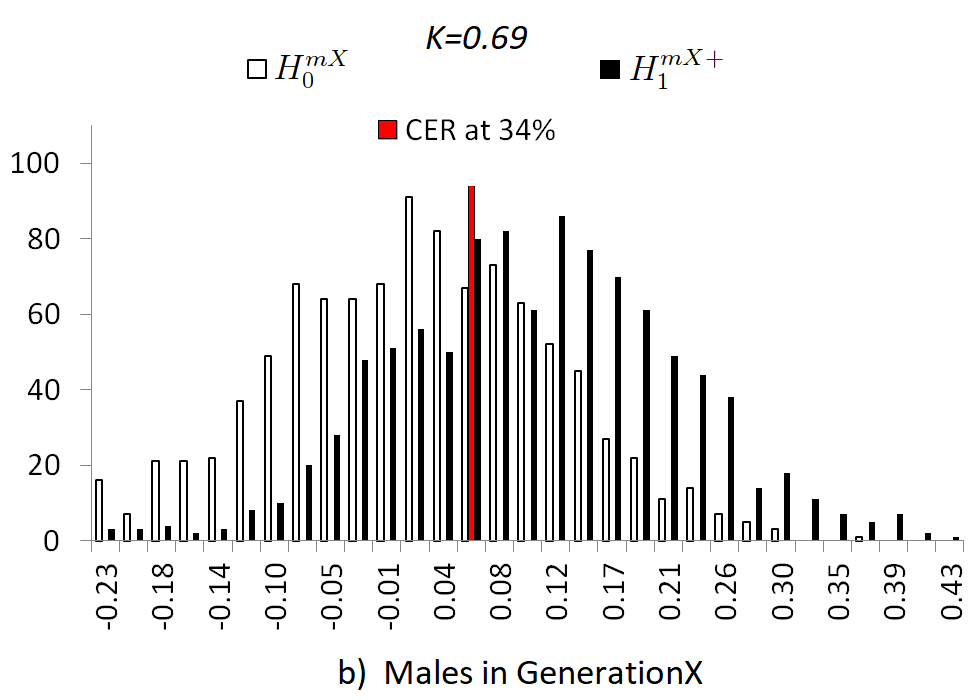
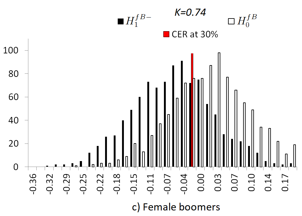
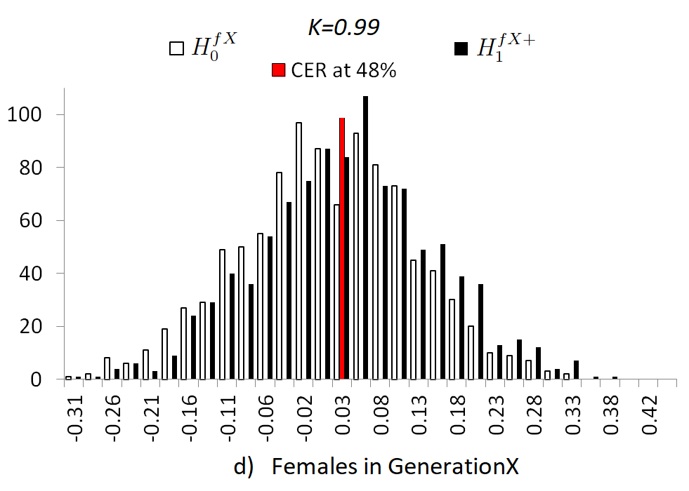
Figure 2: Probability distributions of the net generation effects $({NGE}_{\text{gender},\text{generation},2010,2020})$ under $H_{0}$ and $H_{1}$

Notes: Each of the distributions of ${NGE}_{\text{gender},\text{generation},2010,2020}$ is generated with four binomially distributed random numbers. Each random number represents the number of “very important” responses in a simulated group. E.g. for ${NGE}_{\text{male},\text{Boomers},2010,2020}$, the four groups are (i) the early Boomer males born between 1946 and 1950 and interviewed in 2010, (ii) the late Boomer males born between 1956 and 1960 and interviewed in 2010, (iii) all the male Boomers born between 1946 and 1964 and interviewed in 2010, (iv) all the male Boomers born between 1946 and 1964 and interviewed in 2017. The size of the simulated groups corresponding to the number of trials is set equal to the size of the groups in our sample, while the other parameter of each of the binomial distributions (i.e., the probability of success) is set equal to the corresponding estimated population share of “picky” individuals under $H_{1}$. Under $H_{0}$ of ${NGE}_{\text{gender},\text{generation},2010,2020}=0$, the success rates are set the same for the groups directly compared to make both ${GE}_{\text{gender},\text{generation},2010}=0$ and ${AE}_{\text{gender},\text{generation},2010,7}=0$. E.g. in case of the male Boomers, the success rate in the pair of groups (i) and (ii), as well as in the pair of groups (iii) and (iv), is set equal to the weighted average of their estimated population shares with weights given by the relative sample size. CER is the crossover error rate, i.e., the significance level equating the size of the test of $H_{0}$ with its $\beta$ (=1-power) under $H_{1}$. The Bayes factor $K$ is given by $Pr(D|\text{IPF})/Pr(D|\text{NM})$, where $D$ denotes the observed data.

5 Significance of the results

As we have seen, our survey data analysis facilitates method-selection. Method-selection is seemingly a technical issue. However, it has relevance even for policy-making for the following reasons.

First, the disagreement between the IPF and the NM over the trend of homophily means a disagreement over the trend of a specific, non-monetary dimension of inequality. This is because homophily is an indicator of the perceived width of the social gap between “them” and “us”.

To recall, the disagreements between the two methods are the following. According to the NM and also according to the rich survey data analyzed in this paper, the studied dimension of inequality displayed a U-shaped pattern over the second half of the twentieth century and the first decade of the twenty-first century: there was a period after World War II (i.e., when the late Boomers gradually replaced the early Boomers on the marriage market) that is characterized by the weakening of both the revealed and the self-reported marital homophily. It was followed by another period (i.e., when the late GenerationX gradually replaced the early GenerationX on the marriage market) when both the revealed and the self-reported homophily has been strengthened. In contrast to the NM, the IPF suggests that the trend of the studied dimension of inequality was positive in the first period, while inequality was stagnant in the second period.

Second, one’s view about the effectiveness of certain policies at mitigating inequality and making the society more cohesive may depend on the identified historical trends. Provided the type of inequality analyzed in this paper is quantified to be higher in the generation of the late Boomers than in the generation of the early Boomers despite of the generous welfare policies that the late Boomers could probably benefit from more than the early Boomers, it seems inevitable that we will continue to experience widening social gaps in the future.

However, our view on the future trends can be different if we have reliable evidence for the decline in inequality in the past. So, the significance of our survey-based method-selection is due to the fact that the choice between the IPF and the NM is not innocuous: it makes a difference to what future paths are believed to be possible and also to what policies are believed to have the potential to pave these paths.

Third, there is a growing agreement in the literature about the pattern of some other, but related dimensions of inequality. In particular, there is a forming consensus about the U-curve historical trend of income inequality and wealth inequality. Piketty and Saez (2003), Saez and Zucman (2016) contributed largely to shaping this new consensus. They used American tax records, rather than surveys, to estimate the distribution of income and wealth for a period covering also the decades analyzed in this paper. We stress that the U-curve pattern itself has not been challenged even though there is an ongoing debate in the literature on how steep the decline and the subsequent increase in inequality were (see Bricker, Henriques, Krimmel and Sabelhaus 2016, Auten and Splinter 2022, Geloso, Magness, Moore and Schlosser 2022).

The discourse in the assortative mating literature lags far behind the debate about wealth and income inequality since there is no agreement yet over the qualitative trend of educational homophily and its measurement. Also, there is no consensus about the conditions that any indicator has to satisfy to provide a suitable measure of sorting or homophily.

In order to build consensus in the assortative mating literature, Chiappori, Costa Dias and Meghir (2021) define some simple conditions. While the selective set of empirical examples in this paper also demonstrates the need for a rigorous approach for choosing suitable indicators, we miss the condition of commutativity from the set of conditions they propose. To recall, under this condition, the table-transformation methods preserving any of the indicator commute with the operation of merging neighboring categories of ordered traits. As it is illustrated with the numerical examples in Section 2, this condition is violated by the odds-ratio-based IPF even though the odds-ratio, as a candidate for sorting indicator, satisfies all the simple conditions imposed by Chiappori, Costa Dias and Meghir (2021) (e.g. symmetry) and also their additional condition of having a known structural interpretation.

In contrast to the odds-ratio–IPF pair, the LL-indicator–NM-method duo meets not only some conditions dictated by heuristics and discussed by both Naszodi and Mendonca (2021a) and Chiappori, Costa Dias and Meghir (2021) but also the commutativity condition. In addition, it can be rationalized by the Gale-Shapley matching algorithm at the micro level (see Naszodi and Mendonca 2022, Naszodi and Mendonca 2021b).

It is on our research agenda to study whether the empirical findings in the assortative mating literature of various non-U-shaped trends in sorting or homophily can be attributed to the applied indices violating the commutativity condition and the educational categories chosen. Also, we are going to check in a follow-up paper whether the results of our survey analysis are robust to working with the share of “not at all important” responses given by the most inclusive survey participants rather than the “very important” responses given by the most “picky” group of individuals (see the preliminary results in Naszodi 2022).

6 Conclusion

Population data on couples are informative about a specific dimension of inequality (i.e., the intensity of homophily in a society). However, to identify the changes in this dimension of inequality, one does not only need data on marriages and cohabitations, but also a method appropriate for disentangling “desires” and “opportunities”. The commonly used IPF algorithm and its alternative method, the NM, seem to be natural candidates for performing the related counterfactual decomposition.

In this paper, we highlighted the difference between the two sets of problems these methods were original developed for. In addition, we presented some theoretical considerations on the basis of which it is questionable that the IPF is suitable for constructing counterfactuals in general. Then, we presented an empirical method-selection approach. Our approach is similar to the one proposed by Naszodi and Mendonca (2021a). However, there are some important differences between the two.

Their selection criteria, as well as ours, exploit the fact that the two methods disagree on the relative strength of aggregate revealed preferences in some generations whose aggregate self-reported preferences are known from a survey. The survey data they use is from a single wave. Their survey evidence seem to corroborate the application of the NM. However, this evidence is subject to a criticism: the variation in the self-reported preferences across different generations identified from only one wave of a survey may come partly from the variation of preferences over the course of individuals’ lives.

In this paper, we used survey data from two waves to net the generation-effects from the confounding age-effects. In addition, unlike Naszodi and Mendonca (2021a), we conducted some formal hypothesis tests about the sign and magnitude of the net generation-effects. Our tests provide even more convincing evidence in favor of the U-shaped historical trend of the specific dimension of inequality studied by the assortative mating literature. Thereby, our paper offers even more convincing support for the NM than the survey statistics presented by Naszodi and Mendonca (2021a).

The distribution of survey participants

Let us visit the distribution of survey participants by gender, generation and also by the dichotomous type of respondent–non-respondent. In 2010, the survey question was answered by 289 women and 237 men in the four age groups studied by Naszodi and Mendonca (2021a). Out of the 289 women, 84 were in the age group 60–64 (representing early Boomers), 92 were in the age group 50–54 (representing late Boomers), 60 were in the age group 40–44 (representing early GenerationX) and 53 were in the age group 30–34 (representing late GenerationX). Out of the 237 men respondents, 56 were in the age group 60–64, 75 were in the age group 50–54, 61 were in the age group 40–44, 45 were in the age group 30–34. Answering the survey question was refused by only 3 women (of age 35, 55, and 87 years) and 1 men (of age 57 years).

In 2017, the question was answered by 809 female Boomers and 754 male Boomers (born between 1946–1964); 715 females in GenerationX and 756 males in GenerationX (born between 1965–1980). In the same year, answering the survey question was refused by 3 female Boomers, 2 male Boomers, and by 1 female in GenerationX.

In 2010, the generational distribution of the survey respondents was this: there were 302 female Boomer respondents and 271 male Boomer respondents (born between 1946–1964); 188 female respondents in GenerationX and 176 males respondents in GenerationX (born between 1965–1980). The generational and gender distribution of the survey non-respondents was the following: 1 female Boomer, 1 male Boomer and 1 female in GenerationX.

Detailed empirical results

The results of our empirical analysis are presented by Tables 3 and 4 for the Boomers and the GenerationX, respectively.

Let us first look at the estimates of the population-shares of “picky” individuals among the Boomers (see column 6 in Table 3). Apparently, this share was significantly lower among men in the generation of the late Boomers in 2010 than among men in the generation of the early Boomers in the same year. For women, the population-share of “picky” individuals was not significantly different among the late Boomers and the early Boomers in 2010 since the 60% confidence interval of ${GE}_{\text{female},\text{late and early GenX},2010}$ contains the value zero.

Table 3: The views of the opposite sex in the generation of Boomers on the importance of spousal education

	Generation	Survey	Num.	Num.	Share of	Estimated	Generation-	Age-	Net
		year	of res-	of res-	“picky”	population-	effect	effect	generation-
			ponses	ponses	respon-	share**	with	(older-	effect
				“very	dents*		age-effect	younger)
				impor-			(younger-		(younger-
				tant”			older)		older)
						[60% conf.	[60% conf.	[60% conf.	[60% conf.
						interval]	interval]	interval]	interval]
	(Year of birth)				(in %)	(in %)	(in p.p.)	(in p.p.)	(in p.p.)
		(1)	(2)	(3)	(4)=(3)/(2)	(5)	(6)	(7)	(8)=(6)+(7)$\times$10yrs/7yrs
Male respondents	Late Boomer	2010	75	25	33.3	33.5	} -11.2		-24.2
	(1956-1960)					[28.9;38.1]
	Early Boomer	2010	56	25	44.6	44.7
	(1946-1950)					[39.2;50.3]	[-18.4;-4.0]		[-32.5;-15.9]
	Boomer	2010	271	104	38.4	38.4		} -9.1
	(1946-1964)					[35.9;40.9]
	Boomer	2017	754	221	29.3	29.3
	(1946-1964)					[27.9;30.7]		[-11.9;-6.2]
Female respondents	Late Boomer	2010	92	32	34.8	34.9	} -3.3		-6.6
	(1956-1960)					[30.7;39.1]
	Early Boomer	2010	84	32	38.1	38.2
	(1946-1950)					[33.8;42.6]	[-9.4;2.8]		[-13.9;0.0]
	Boomer	2010	302	116	38.4	38.4		} -2.3
	(1946-1964)					[36.1;40.8]
	Boomer	2017	809	292	36.1	36.1
	(1946-1964)					[34.7;37.5]		[-5.1;0.0]

Notes: *Proportion of women among the survey respondents in a given generation who said that it is a very important quality of a good husband/partner to be well-educated; or, proportion of men who said that it is a very important quality of a good wife/partner to be well-educated. **Calculated by the approximation proposed by Agresti and Coull (1998). The correlations are assumed to be zero between the empirical shares in 2010 and 2017 among those belonging to the same generation.
Source: Changing American Family survey and The American Trends Panel Wave 28 survey conducted by the Pew Research Center in 2010 and 2017, respectively (see: https://www.pewsocialtrends.org/dataset/changing-american-family/ and https://www.pewsocialtrends.org/dataset/american-trends-panel-wave-28/).

Next, let us visit the age-effect of the Boomers (see column 7 of Table 3). It informs us about how the Boomers’ responses have changed over seven years between 2010 and 2017. The age-effect is negative both for men and women. So, as the Boomers get older, fewer of them tend to report education to be a very important spousal trait.

Accordingly, the late Boomer men are found to be even less “picky” about spousal education than the early Boomer men on average, once the age-effect is controlled for (see column 8 in the upper part of Table 3). As to the confidence interval of the net generation-effect of male Boomers, its upper bound is decreasing in the correlation $\rho$. It is -15.9% for the unreasonably low value of zero correlation (see column 8 in the upper part fo Table 3), while it is -16.8% for the other extreme of perfect correlation. The p-value is as low as 0.7% when the correlation is calibrated to zero. Whereas it is 0.2% for the correlation calibrated to one. So, irrespective of the correlation’s value, we can reject $H^{mB}_{0}$ in favor of $H^{mB-}_{1}$ at any meaningful significance level.

For women, the adjustment with the age-effect results in a confidence interval of the net generation-effect that is entirely in the negative range if the correlation is one. However, it contains the value zero in the benchmark case of zero correlation (see column 8 in the lower part fo Table 3). The p-value is 18.5% if the correlation is one, while it is 22% if the correlation is zero.

So, we can reject $H^{fB}_{0}$ at any significance level above 22%, irrespective of the calibrated value of $\rho$. As a reference of comparison of the 22%, we calculate the crossover error rate, i.e., the significance level that equates the size of the test of $H^{fB}_{0}:{NGE}_{\text{female},\text{Boomers}}=0$ with its $\beta$ (=1-power) under the alternative of $H^{fB-}_{1}:{NGE}_{\text{female},\text{Boomers}}=-6.6$ pp. It is higher than 22% as it is 30% (see Fig. 2c).

Finally, it is worth to note that even if we set the bound on the Type I error lower than 22% (at the cost of increasing the probability of the Type II error above 45%) and accept $H^{fB}_{0}$, our tests for the male Boomers and the female Boomers together clearly support the application of the NM for constructing counterfactuals. This is because revealed homophily should be found to be weaker among the late Boomers relative to the early Boomers even if only the late Boomer males’ self-reported preferences are found to be weaker than that of the early Boomer males, while the self-reported preferences of the late and early Boomer females are found similar.

Let us turn to the survey responses of the GenerationX. Similarly to the age-effects of the Boomers, the age-effects for men and women are negative in the GenerationX. So, as the members of the GenerationX get older, fewer of them tend to report education to be a very important spousal trait (see column 7 in Table 4). Therefore, the adjustment with the age-effects works against accepting $H^{mX+}_{1}$ and $H^{fX+}_{1}$. For instance, the point estimates of males’ generation-effect is $\widehat{GE}_{\text{males},\text{late and early GenX},2010}=13.2\%$, whereas their net generation-effect (i.e., the generation-effect adjusted with the age-effect) is lower. The latter is $\widehat{NGE}_{\text{males},\text{late and early GenX},2010,2020}=9.8\%$ (see columns 6 and 8 in the upper part of Table 4).

Still, despite the negative sign of the estimated age-effect, the point estimates of males’ net generation-effect suggests that the share of “picky” men would have been substantially higher (by almost 10 pp) in the late GenerationX relative to the early GenerationX provided the members of these generations had been observed at the same age.

As to the confidence interval of ${NGE}_{\text{males},\text{late and early GenX},2010,2020}$, it is in the positive range. Its lower bound is increasing in $\rho$. The lower bound is 0.4% for the unreasonably low value of zero correlation (see column 8 in the upper part of Table 4), while it is 1.5% for the intuitively more reasonable other extreme of perfect correlation. So, we can reject $H^{mX}_{0}$ at the 20% significance level in favor of $H^{mX+}_{1}$ even under the zero correlation assumption. (The p-value is 18.9% under zero correlation, whereas it is 16.1% under perfect correlation. As it is shown by Fig. 2b, the crossover error rate is around 34%.)

By contrast, we cannot reject $H^{fX}_{0}$ against $H^{fX+}_{1}$ for women at any significance level lower than 20% since the 60% symmetric confidence interval of their net generation-effect contains the value zero (see column 8 in the lower part of Table 4).

To conclude, although women’s declared preferences do not seem to have changed as remarkably as men’s self-reported preferences did across the generations studied, we find the late Boomers to be less “picky” overall than the early Boomers, while we find the late GenerationX to be much more “picky” overall than the early GenerationX because of the change in preferences at the men’s side of the marriage market. These results validate the NM.

Table 4: The views of the opposite sex in the GenerationX on the importance of spousal education

	Generation	Survey	Num.	Num.	Share of	Estimated	Generation-	Age-	Net
		year	of res-	of res-	“picky”	population-	effect	effect	generation-
			ponses	ponses	respon-	share**	with	(older-	effect
				“very	dents*		age-effect	younger)
				impor-			(younger-		(younger-
				tant”			older)		older)
						[60% conf.	[60% conf.	[60% conf.	[60% conf.
						interval]	interval]	interval]	interval]
	(Year of birth)				(in %)	(in %)	(in p.p.)	(in p.p.)	(in p.p.)
		(1)	(2)	(3)	(4)=(3)/(2)	(5)	(6)	(7)	(8)=(6)+(7)$\times$10yrs/7yrs
Male respondents	Late GenX	2010	45	20	44.4	44.5	} 13.2		9.8
	(1976-1980)					[38.3;50.7]
	Early GenX	2010	61	19	31.1	31.4
	(1966-1970)					[26.4;36.3]	[5.2;21.1]		[0.4;19.1]
	GenX	2010	176	67	38.1	38.1		} -2.4
	(1965-1980)					[35;41.2]
	GenX	2017	756	270	35.7	35.7
	(1965-1980)					[34.3;37.2]		[-5.8; 0.0]
Female respondents	Late GenX	2010	53	24	45.3	45.3	} 5.2		2.7
	(1976-1980)					[39.6;51.1]
	Early GenX	2010	60	24	40.0	40.1
	(1966-1970)					[34.8;45.4]	[-2.6;13.0]		[-6.5;11.8]
	GenX	2010	188	78	41.5	41.5		} -1.8
	(1965-1980)					[38.5;44.5]
	GenX	2017	715	284	39.7	39.7
	(1965-1980)					[38.2;41.3]		[-5.2;1.6]

Notes: same as under Table 3.

Table 5: The views of the opposite sex in the generation of Boomers on the importance of spousal education – perfect correlation

	Generation	Survey	Num.	Num.	Share of	Estimated	Generation-	Age-	Net
		year	of res-	of res-	“picky”	population	effect	effect	generation-
			ponses	ponses	respon-	share**	with	(older-	effect
				“very	dents*		age-effect	younger)
				impor-			(younger-		(younger-
				tant”			older)		older)
						[60% conf.	[60% conf.	[60% conf.	[60% conf.
						interval]	interval]	interval]	interval]
	(Year of birth)				(in %)	(in %)	(in p.p.)	(in p.p.)	(in p.p.)
		(1)	(2)	(3)	(4)=(3)/(2)	(5)	(6)	(7)	(8)=(6)+(7)$\times$10yrs/7yrs
Male respondents	Late Boomer	2010	75	25	33.3	33.5	} -11.2		-24.2
	(1956-1960)					[28.9;38.1]
	Early Boomer	2010	56	25	44.6	44.7
	(1946-1950)					[39.2;50.3]	[-18.4;-4.0]		[-31.5;-16.8]
	Boomer	2010	271	104	38.4	38.4		} -9.1
	(1946-1964)					[35.9;40.9]
	Boomer	2017	754	221	29.3	29.3
	(1946-1964)					[27.9;30.7]		[-10.2;-8]
Female respondents	Late Boomer	2010	92	32	34.8	34.9	} -3.3		-6.6
	(1956-1960)					[30.7;39.1]
	Early Boomer	2010	84	32	38.1	38.2
	(1946-1950)					[33.8;42.6]	[-9.4;2.8]		[-12.9;-0.4]
	Boomer	2010	302	116	38.4	38.4		} -2.3
	(1946-1964)					[36.1;40.8]
	Boomer	2017	809	292	36.1	36.1
	(1946-1964)					[34.7;37.5]		[-3.3;-1.4]

Notes: same as under Table 3 except that parameter $\rho$ (the correlation between the empirical shares of the “picky” individuals belonging to the same generation while being observed in 2010 and 2017) is calibrated to one.

Table 6: The views of the opposite sex in the GenerationX on the importance of spousal education – perfect correlation

	Generation	Survey	Num.	Num.	Share of	Estimated	Generation-	Age-	Net
		year	of res-	of res-	“picky”	population	effect	effect	generation-
			ponses	ponses	respon-	share**	with	(older-	effect
				“very	dents*		age-effect	younger)
				impor-			(younger-		(younger-
				tant”			older)		older)
						[60% conf.	[60% conf.	[60% conf.	[60% conf.
						interval]	interval]	interval]	interval]
	(Year of birth)				(in %)	(in %)	(in p.p.)	(in p.p.)	(in p.p.)
		(1)	(2)	(3)	(4)=(3)/(2)	(5)	(6)	(7)	(8)=(6)+(7)$\times$10yrs/7yrs
Male respondents	Late GenX	2010	45	20	44.4	44.5	} 13.2		9.8
	(1976-1980)					[38.3;50.7]
	Early GenX	2010	61	19	31.1	31.4
	(1966-1970)					[26.4;36.3]	[5.2;21.1]		[1.5;18]
	GenX	2010	176	67	38.1	38.1		} -2.4
	(1965-1980)					[35;41.2]
	GenX	2017	756	270	35.7	35.7
	(1965-1980)					[34.3;37.2]		[-4; -0.8]
Female respondents	Late GenX	2010	53	24	45.3	45.3	} 5.2		2.7
	(1976-1980)					[39.6;51.1]
	Early GenX	2010	60	24	40.0	40.1
	(1966-1970)					[34.8;45.4]	[-2.6;13.0]		[-5.4;10.7]
	GenX	2010	188	78	41.5	41.5		} -1.8
	(1965-1980)					[38.5;44.5]
	GenX	2017	715	284	39.7	39.7
	(1965-1980)					[38.2;41.3]		[-3.3;-0.3]

Notes: same as under Table 5.

References

- (1)
- Agresti and Coull (1998) Agresti, A. and B. A. Coull (1998), Approximate is better than "exact" for interval estimation of binomial proportions, The American Statistician, 52 (2), 119–126.
- Auten and Splinter (2022) Auten, G. and D. Splinter (2022), Income inequality in the United States: Using tax data to measure long-term trends (Working Paper).
- Becker (1973) Becker, G. S. (1973), A theory of marriage: Part I, Journal of Political Economy, 81 (4), 813–846.
- Biewen (2014) Biewen, M. (2014), A general decomposition formula with interaction effects, Applied Economics Letters, 21, 636–642.
- Bricker, Henriques, Krimmel and Sabelhaus (2016) Bricker, J., A. Henriques, J. Krimmel and J. Sabelhaus (2016), Estimating top income and wealth shares: Sensitivity to data and methods, American Economic Review, 106 (5), 641–45.
- Chiappori, Costa Dias and Meghir (2021) Chiappori, P.-A., M. Costa Dias and C. Meghir (2021), The measuring of assortativeness in marriage: A comment. Cowles Foundation Discussion Paper(2316).
- Chiappori, Costa Dias and Meghir (2020) Chiappori, P.-A., M. Costa Dias and C. Meghir (2020), Changes in Assortative Matching: Theory and Evidence for the US. National Bureau of Economic Research, Working Paper Series, no. 26932.
- Choo and Siow (2006) Choo, E. and A. Siow (2006), Who marries whom and why, Journal of Political Economy, 114 (1), 175–201.
- Eika, Mogstad and Zafar (2019) Eika, L., M. Mogstad and B. Zafar (2019), Educational assortative mating and household income inequality, Journal of Political Economy.
- Geloso, Magness, Moore and Schlosser (2022) Geloso, V. J., P. Magness, J. Moore and P. Schlosser (2022), How pronounced is the U-curve? Revisiting income inequality in the United States, 1917–60, The Economic Journal, 132 (647), 2366–2391.
- Hitsch, Hortaçsu and Ariely (2010) Hitsch, G. J., A. Hortaçsu and D. Ariely (2010), What Makes You Click? - Mate Preferences in Online Dating, Quantitative Marketing and Economics, 8 (4).
- Kalmijn (1998) Kalmijn, M. (1998), Intermarriage and homogamy: Causes, patterns, trends, Annual Review of Sociology, 24, 395–421.
- Lichter and Qian (2019) Lichter, D. and Z. Qian (2019), The study of assortative mating: Theory, data, and analysis. In R. Schoen (Ed.), Analytical Family Demography (Vol. 47). Springer, Cham.
- Liu and Lu (2006) Liu, H. and J. Lu (2006), Measuring the degree of assortative mating, Economics Letters, 92 (3), 317–322.
- Meyer (1980) Meyer, M. M. (1980), Generalizing the iterative proportional fitting procedure (Technical Report No. 371). University Minnesota.
- Mood (2010) Mood, C. (2010), Logistic regression: Why we cannot do what we think we can do, and what we can do about it?, European Sociological Review, 26, 67–82.
- Naszodi (2022) Naszodi, A. (2022), The iterative proportional fitting algorithm and the NM-method: solutions for two different sets of problems , Arxiv.org, .
- Naszodi (2023) Naszodi, A. (2023), Direct comparison or indirect comarison via a series of counterfactual decompositions?, Arxiv.org, https://doi.org/10.48550/arXiv.2303.04905.
- Naszodi and Mendonca (2019) Naszodi, A. and F. Mendonca (2019), Like marries like, JRC Science for Policy Briefs Series, European Commission, Joint Research Centre, JRC115102, March https://knowledge4policy.ec.europa.eu/sites/default/files/fairness_pb2019_assortative_mating_jrc115102.pdf.
- Naszodi and Mendonca (2021a) Naszodi, A. and F. Mendonca (2021a), A new method for identifying the role of marital preferences at shaping marriage patterns, Journal of Demographic Economics, 1–27. https://doi.org/10.1017/dem.2021.1
- Naszodi and Mendonca (2021b) Naszodi, A. and F. Mendonca (2021b), A new method for identifying what Cupid’s invisible hand is doing. Is it spreading color blindness while turning us more “picky” about spousal education?, Arxiv.org, https://arxiv.org/abs/2103.06991.
- Naszodi and Mendonca (2022) Naszodi, A. and F. Mendonca (2022), Changing educational homogamy: Shifting preferences or evolving educational distribution?, Journal of Demographic Economics, 1–29. https://doi.org/10.1017/dem.2022.21
- Piketty and Saez (2003) Piketty, T. and E. Saez (2003), Income inequality in the United States, 1913–1998, The Quarterly Journal of Economics, 118 (1), 1–41.
- Saez and Zucman (2016) Saez, E. and G. Zucman (2016), Wealth inequality in the United States since 1913: Evidence from capitalized income tax data, The Quarterly Journal of Economics, 131 (2), 519–578.
- Stephan and Deming (1940) Stephan, F. F. and W. E. Deming (1940), On a least squares adjustment of a sampled frequency table when the expected marginal totals are known, The Annals of Mathematical Statistics, 11 (4), 427–444.
Appendix