Stability Results for Novel Serially-connected Magnetizable Piezoelectric and Elastic Smart-System Designs
Abstract.
In this paper, the stability of longitudinal vibrations for transmission problems of two smart-system designs are studied: (i) a serially-connected Elastic-Piezoelectric-Elastic design with a local damping acting only on the piezoelectric layer and (ii) a serially-connected Piezoelectric-Elastic design with a local damping acting on the elastic part only. Unlike the existing literature, piezoelectric layers are considered magnetizable, and therefore, a fully-dynamic PDE model, retaining interactions of electromagnetic fields (due to Maxwell’s equations) with the mechanical vibrations, is considered. The design (i) is shown to have exponentially stable solutions. However, the nature of the stability of solutions of the design (ii), whether it is polynomial or exponential, is dependent entirely upon the arithmetic nature of a quotient involving all physical parameters. Furthermore, a polynomial decay rate is provided in terms of a measure of irrationality of the quotient. Note that this type of result is totally new (see Theorem 3.6 and Condition ). The main tool used throughout the paper is the multipliers technique which requires an adaptive selection of cut-off functions together with a particular attention to the sharpness of the estimates to optimize the results.
Keywords. magnetizable piezoelectric beams; serially-connected beams; transmission problems; irrationality measure; partial viscous damping; exponential stability; polynomial stability.
1. Introduction
Piezoelectric materials are multi-functional smart materials (most notably Lead Zirconate Titanate) used to develop electric displacement that is directly proportional to an applied mechanical stress [49]. They can be used as actuators/sensors, and also be integrated to a mother host structure [48]. Due to their small size and high power density, they have become more and more promising in industrial applications such as implantable biomedical devices and sensors [14, 15], wearable human-machine interface sensors [16], and nano-positioners and micro-sensors due to the excellent advantages of the fast response time, large mechanical force, and extremely fine resolution [45].
In deriving a mathematical model for the equations of motion on a piezoelectric beam, actuated by a voltage source, three major effects and their interrelations need to be considered: mechanical, electrical, and magnetic. Mechanical effects are mostly modeled through Kirchhoff, Euler-Bernoulli, or Mindlin-Timoshenko small (linear) [28] or large (nonlinear) [18] displacement assumptions, where the constitutive relations between the nonzero stress and strain tensors are used to model longitudinal displacements of the centerline (stretching/compression), transverse displacements (bending), and rotations of the beam. It is also reported that the small displacement assumptions lead to the bending and rotational motions completely immune the applied voltage [36]. These tensors are coupled to the electric/magnetic displacements and electric/magnetic field tensors. There are mainly three approaches to include electromagnetic effects due the Maxwell’s equations: electrostatic, quasi-static, and fully-dynamic [25, p. 336]. Electrostatic and quasi-static approaches are widely used in voltage-controlled piezoelectric beam models - see e.g. [49] and the references therein. These models completely exclude magnetic effects and their coupling with electrical and mechanical effects. Even though the electro-static and quasi-static approaches are sufficient for defining piezoelectricity, electromagnetic waves generated by mechanical fields need to be accounted for in the calculation of radiated electromagnetic power from a vibrating piezoelectric acoustic device, e.g. see [53] and the references therein. For this reason, the fully dynamic models of piezoelectric beams are needed to be understood well. In fact, the dynamic effects for (acoustic) magnetizable piezoelectric beams are pronounced and must be taken into account in the modeling [36, 50].
Denote and by the longitudinal vibrations of the center line of the beam and the total charge accumulated at the electrodes of a single piezoelectric beam. Assuming that the beam is fixed at the left end and free at the right end , the equations of motion is a system of partial differential equations [36] as the following
| (1.1) |
where , , , , and are mass density per unit volume, elastic stiffness, impermeability, piezoelectric constant, and magnetic permeability of the beam, respectively, and and are strain and voltage actuators, and
| (1.2) |
By the electrostatic approach, the model above is simplified to a single wave equation model by taking and considering and (1.2), e.g. see [37],
| (1.3) |
The model by the quasi-static approach is the same as (1.3) yet
The exact observability/stabilizability and the type of stability of the solutions (1.1) of the PDE model by each approach differs substantially. For example, the PDE model obtained by electrostatic/quasi-static approach is the boundary damped wave equation in (1.3), and it is known to be exactly observable/exponentially stabilizable with one state measurement on the boundary , e.g. see [12, 24]. In deep contrast to this result, the PDE model obtained by the the fully-dynamic approach in (1.1) can not be exactly observable/exponentially stabilizable for almost all choices of material parameters with only one state measurement, or on the boundary , e.g. see [36, 37]. Explicit polynomial decay estimates are obtained for more regular initial data and for a small class of materials satisfying certain number-theoretical conditions [37, 38]. The same model (1.1) is considered in [41] for the open-loop sensor configuration (i.e. ) with a dissipative damping term with acting only in the first equation of (1.1). It is also reported that two nonzero state feedback measurements (tip velocity) and (total current on the electrodes) are necessary to achieve exact observability/exponential stabilizability [42, 52]. This underlines the fact that the two boundary damping terms or one viscous damping term are both able to exponentially dissipate non-stabilizing (high-frequency) magnetic effects. There is also a large literature considering the model (1.1) under thermal effects, fractional-type damping, and distributed or boundary-type memory and delay terms, see [2]-[5],[17]-[22], [47, 54] and the references therein.
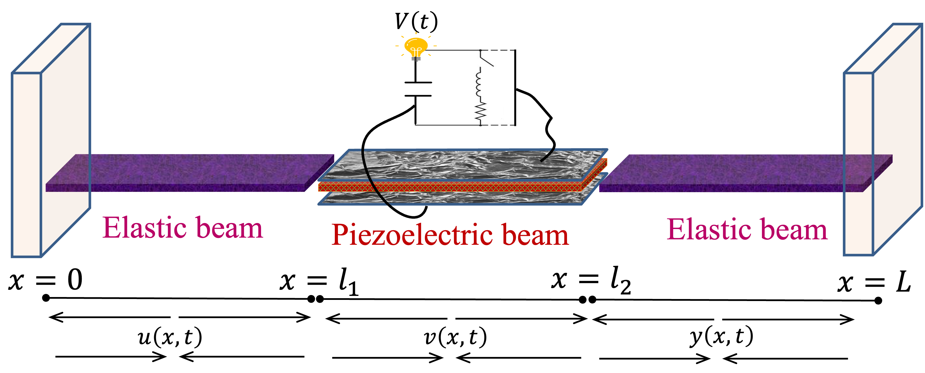
A serially-connected smart system is an elastic structure consisting of longitudinally attached fully-elastic and piezoelectric layers, see Figs. 1 and 2. Use of piezoelectric materials for a serially-connected design in various transmission mechanisms of aerospace, aviation, automobile, ships, and robots has boosted substantially in the last decade, see [13, 30] and the references therein. A rigorous mathematical treatment for a transmission problem of a three serially-connected purely-elastic waves/strings/beams is provided in [20]. Indeed, if the outer wave equations have both viscous damping terms, an exponential stability result is shown to be immediate. Several authors have also studied transmission problems of serially-connected strings/beams with e.g. a thermoelastic material [35] or a viscoelastic material [43].
To the best of our best knowledge, serially-connected transmission systems involving elastic and magnetizable piezoelectric systems are not treated mathematically in the literature, especially with Condition , which appears in Section 3.3. The goal of this paper is to fix this gap by considering two particular designs, for which we obtain novel decay rates of the energy, see Theorems 2.6, 3.5 and 3.6. The first design, whose PDE model is described below in (), is the transmission problem of an Elastic-Piezoelectric-Elastic system, as in Fig. 1, with only one local damping acting on the longitudinal displacement of the center line of the piezoelectric material:
| () |
where , and , such that
| () |
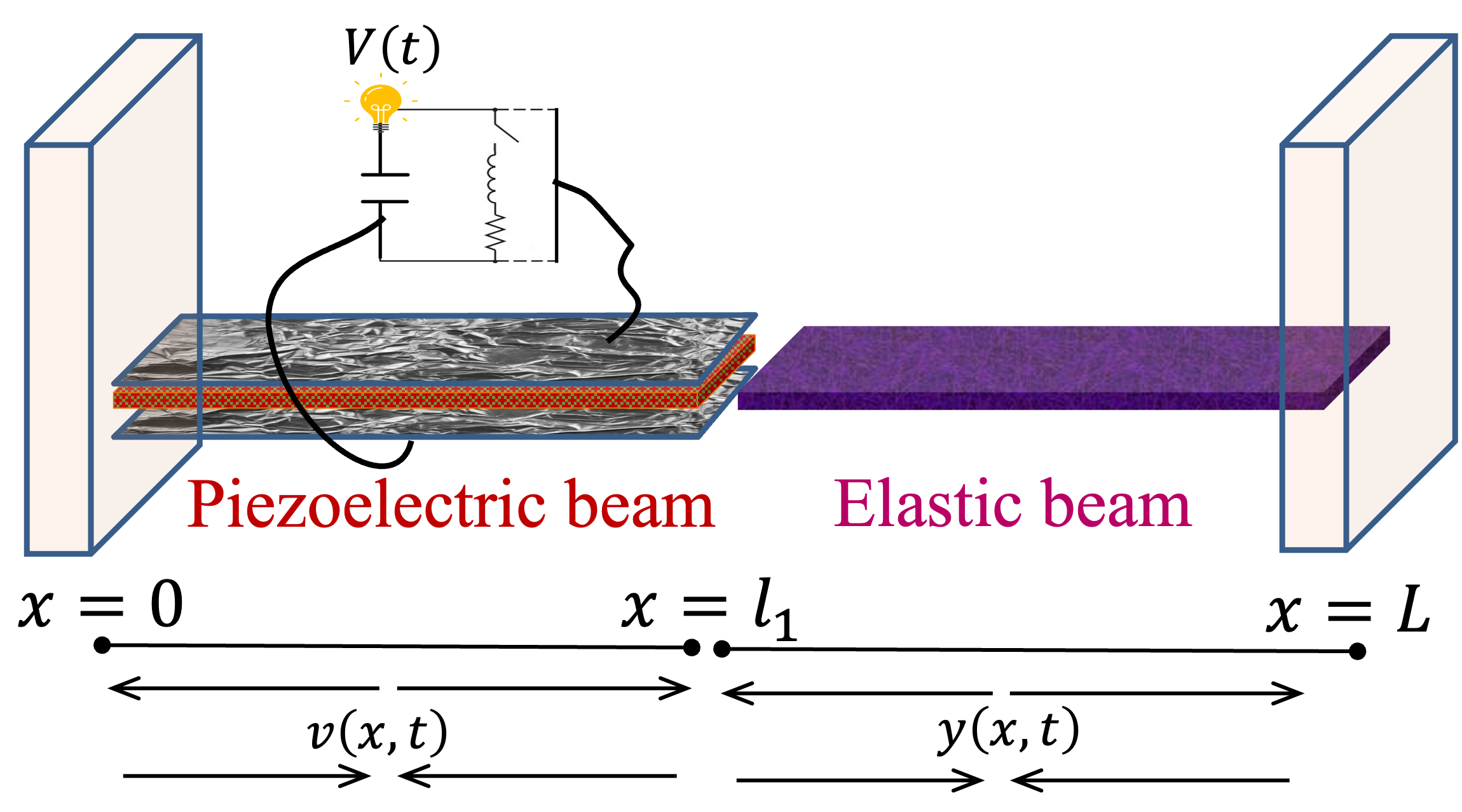
The second design, whose PDE model is described below in (), is for the transmission problem of a Piezoelectric-Elastic system, as in Fig. 2, with only one local damping acting on the elastic part:
| () |
where , and such that
| () |
The paper is organized as follows. In Section 2, first, well-posedness and the exponential stability of the model () are studied under the conditions () on the damping function . In Section 3, the well-posedness and the strong stability of () system are analyzed under the conditions () on the damping function . Moreover, the decay rate of the energy depends on the arithmetic nature of a quotient involving all physical parameters of the system. More precisely, if the quotient is a rational number different from , for all ( see () in Theorem 3.3), the energy is proved to decay exponentially. If the quotient is an irrational number, the energy is proved to decrease polynomially if the irrationality measure of this quotient is finite. The proof of the main results are all based on the multipliers technique, requiring an adapted choice of cut-off functions, and a particular attention to the sharpness of the estimates to optimize the results.
It is crucial to note that, as a consequence of our arguments developed in section 2, the electrostatic/quasi-static design, identical to the design in [20], with a local damping only acting in the middle layer can be shown to be exponentially stable, see Remark 2.15. This is a major improvement of the results in [20] since the exponential stability result is only achieved by fully-distributed viscous damping terms for the outer layers.
2. Stability results for the () system
Note that the assumption () applies to all results in this section. For simplicity, the repetition is avoided unless it is necessary to state.
2.1. Well-Posedness
This section is devoted to establish the well-posedness of the system () by a semigroup approach. The natural energy of system () is defined by
Proof. First, multiplying by , integrate by parts over and take the real part to get
| (2.2) |
Next, multiply by , integrate by parts over and take the real part to get
| (2.3) |
Now, multiply by , integrate by parts over , and take the real part to get
By implementing and
| (2.4) |
and multiplying by and integrating by parts over lead to
| (2.5) |
Thus, by adding (2.3) and (2.4) and noting (1.2),
| (2.6) |
In the final step of the proof, add (2.2), (2.5) and (2.6), use the continuity conditions and and the transmission conditions and Hence, (2.1) follows.
In order to have a unique solution to (), the following Hilbert spaces are introduced. For any real numbers such that ,
The energy space is now defined by
and for , a norm on can be chosen of the following form
| (2.7) |
noting that the standard norm on is
| (2.8) |
Lemma 2.2.
Proof. The inequality on the right with is immediate by Young’s inequality since
We have and by the transmission condition
Applying Young’s and Cauchy-Schwarz inequalities leads to
| (2.10) | |||
| (2.11) |
As(2.10) and (2.11) are considered together
| (2.12) |
Next, Young’s inequality is applied to get
| (2.13) |
By combining (2.12) and (2.13)
Hence,this leads to the left inequality of (2.9) with
Define the unbounded linear operator by
with the domain
Remark 2.3.
Using (1.2), direct calculations show that the transmission conditions
are equivalent to the transmission conditions
while the transmission conditions
are equivalent to the transmission conditions
If is a sufficiently regular solution of the system (), it can be transformed into a first-order evolution equation on the Hilbert space as the following
| (2.14) |
where and . By the arguments of Lemma 2.1, for all ,
| (2.15) |
which implies that is dissipative. Now, let . By the Lax-Milgram Theorem, one can prove the existence of solving the eequation
Therefore, the unbounded linear operator is dissipative in and consequently, . Moreover, generates a semigroup of contractions , by the Lumer-Phillips theorem. Therefore, the solution of the Cauchy problem (2.14) admits the following representation
which leads to the well-posedness of (2.14). The following result is immediate.
2.2. Strong Stability
Theorem 2.5.
The semigroup of contraction is strongly stable in ; i.e., for all , the solution of (2.14) satisfies
Proof. Since the resolvent of is compact in , it follows from the Arendt-Batty’s theorem (see page 837 in [6]) that the system () is strongly stable if and only if does not have pure imaginary eigenvalues, i.e. . From Section 2.1, it is already know that . Therefore, only must be proved. For this purpose, suppose that there exists a real number and such that
| (2.16) |
which is equivalent to the following system
| (2.17) |
and
| (2.18) |
| (2.19) |
On the other hand, from (2.17), (2.19), () and the fact that , we have
| (2.20) |
By and (2.20) in ,
| (2.21) |
Combining and (2.21) leads to
| (2.22) |
Next, by (2.20) in (2.22) and we get in , the third equation in (2.17) yields
| (2.23) |
Since ,
| (2.24) |
Now, combining (2.22) and , the following reduced system is obtained
| (2.25) | |||||
| (2.26) |
Let . From (2.24), . Now, the system (2.25)-(2.26) can be written in as the following
| (2.27) |
where
The solution of the differential equation (2.27) is given by
| (2.28) |
Analogously, it can be proved that in . Consequently, in . Since ,
| (2.29) |
By , the continuity and transmission conditions,
| (2.30) |
Finally, by , and (2.30) it is easy to conclude that in and in . Hence, . The proof is thus complete.
2.3. Exponential Stability
The aim of the subsection is to prove the exponential stability of System () under the sole assumption (). The main result of this section is the following theorem.
Theorem 2.6.
Before diving into the technicality of the proof of Theorem , recall from, e.g. [27], [40], that a semigroup of contractions on must satisfy two conditions (3.17) if
| () |
| () |
Since we already proved in Theorem 2.5 that , condition () is satisfied. Now only the condition () must be proved. We follow a contradiction argument, for this purpose, suppose that () is false, then there exists with
| (2.32) |
such that
| (2.33) |
For simplicity, let the index be dropped. Then, (2.33) is equivalent to
| (2.34) |
and
| (2.35) |
Merging (2.34) and (2.35), a more compact system of equations is obtained
| (2.36) |
where
| (2.37) |
By in ,
Now, combining and the above equality lead to
Inserting the above equation in , the system is reduced to
| (2.38) |
where
| (2.39) |
At this moment, the following series of technical lemmas, as consequences of the dissipativity property of the solutions of the system (2.34)-(2.35), are needed to finish the proof of Theorem .
Proof. To get the first estimate in (2.40), take the inner product of (2.33) with in , and use and so that
| (2.41) |
Next, by multiplying by , using the first estimation in (2.40), and , the second estimate in (2.40) is immediate. Finally, by () and the second estimate in (2.40), the third estimate in (2.40) is obtained.
Note that for all , the following cut-off functions are fixed
-
, such that , for all and
Observe that on the support of .
Lemma 2.8.
Proof. First, multiply by , integrate over by parts, and use definition of to get
| (2.43) |
It is known that and which implies in particular that is uniformly bounded in due to ). Therefore, by Cauchy-Schwarz inequality, Lemma 2.7, the definition of the following is deduced
Inserting the above estimates into (2.43) and taking the real part leads to
| (2.44) |
Analogously, multiply by , integrate over by parts to get
| (2.45) |
By the definition of , , Cauchy-Schwarz inequality, Lemma 2.7
| (2.46) |
Inserting the estimates above into (2.45) together with Lemma 2.7 yields
| (2.47) |
Thus, the combination of (2.44) and (2.47) gets the first estimate in (2.42), and together with which, and the definition of , the second estimate in (2.42) is immediate. Finally, by the second estimate in (2.42), and the fact that , the third estimate in (2.42) is obtained.
Proof. Multiplying by and integrating over by parts yield
| (2.49) |
By Cauchy-Schwarz inequality, Lemma 2.7, the definition of , and , the following hold
Finally, inserting these estimates in (2.49) and by (2.40), the first estimate, and therefore the second estimate, in (2.48) are obtained.
Lemma 2.10.
Proof. Multiplying by integrating over by parts lead to
| (2.51) |
By Cauchy-Schwarz inequality, Lemmas 2.7, 2.9, the definition of , and ,
Finally, inserting the above estimates into (2.51) and by Lemma 2.8, the first estimate, and therefore the second estimate, in (2.50) are obtained.
Lemma 2.11.
Proof. First, multiply by , and integrate over to get
By several integration by parts and the definition of in (2.37), the following is obtained
| (2.54) |
Since is uniformly bounded in and , by Cauchy-Schwarz inequality and Lemma 2.7
Substituting the estimatation above into (2.54) leads to
| (2.55) |
Analogously, multiply by and integrate over to obtain and taking the real part, we get
By several integration by parts and the definition of given in (2.37), the following holds
| (2.56) |
Since and are uniformly bounded in and Cauchy-Schwarz inequality is implemented to obtain
Substituting the estimates above into (2.56) results in
| (2.57) |
Finally, adding (2.55) and (2.57), the desired result (2.52) is obtained.
Proof. First, define two cut-off functions such that for all and
| (2.59) |
By taking , it is easy to see that
Setting and considering defined above in (2.52) lead to
| (2.60) |
Now, adopting (2.40), (2.42), (2.48), (2.50), the definitions of and and Cauchy-Schwarz inequality result in
| (2.61) |
On the other hand, since , it is easy to see that
| (2.62) |
Therefore, substitution of (2.61) and (2.62) into (2.60) result in
| (2.63) |
Finally, by (2.40), (2.42), (2.48), (2.50), the definitions of and in (2.63), the desired result (2.58) is obtained.
Proof. Define such that
| (2.65) |
By using in (2.52),
| (2.66) |
which, together with (2.65) and (2.58), implies that
Substituting these estimates into (2.66) and by (2.53) leads to
where
| (2.67) |
and therefore,
| (2.68) |
Now, use the fact that and (cf. (2.33)), to obtain
| (2.69) |
Finally, by (2.69), the definition of given in (2.53), and Young’s inequality,
| (2.70) |
where . To get the desired result (2.64), substitute (2.70) into (2.68) and use ,
| (2.71) |
Proof. First, multiply and by and , and integrate over and , respectively. Since and and are uniformly bounded in and , respectively,
and
Since and and are uniformly bounded in and , respectively,
| (2.73) |
and
| (2.74) |
Recalling Remark 2.3, , , (2.64) and the facts that
the following is obtained
Finally, substitution of the estimates above into (2.73) and (2.74), the desired result (2.72) is obtained. Now, we are ready to finally prove Theorem 2.6. Proof of Theorem 2.6. By (2.58) and (2.72), we obtain that . This contradicts that . Hence, () holds true, and this makes the proof complete.
Remark 2.15.
Note that the electrostatic/quasi-static approaches in modeling piezoelectric beams discard the dynamic electromagnetic effects, i.e. in (). Therefore, the reduced model becomes identical to the one obtained in [20], where two fully-distributed viscous damping terms for the outer wave equations are considered to achieve exponential stability. However, through the analysis of the section, it can be shown that only a local damping acting in the middle layer can also lead to an exponential stability result with the assumption (). The proof is exactly the same (even simpler) as the one presented above yet it left to the reader. This is a major improvement of the earlier result.
3. Stability results for the system ()
Note that the assumption () applies to all results in this section. For simplicity, the repetition of the assumption in the results below is avoided unless it is necessary to state.
3.1. Well-Posedness
In this section, the well-posedness of the system () is established by a semigroup approach. The natural energy of the system () is defined by
It is straightforward to show that the energy is dissipative along the smooth enough solutions of (), i.e.
| (3.1) |
Define the energy space
equipped by the norm
| (3.2) |
This norm is equivalent to the standard norm of (the arguments in the proof of Lemma 2.2 can be followed mutatis mutandis). Define the unbounded linear operator by
with the domain
Remark 3.1.
Obviously as in the previous section, the transmission conditions
are equivalent to the transmission conditions
If is a sufficiently regular solution of the system (), the system can be transformed into the first order evolution equation on the Hilbert space
| (3.3) |
with and . By the analogous arguments in Subsection 2.1, the solution of the Cauchy problem (3.3) admits the following representation
which leads to the well-posedness for (3.3).
3.2. Strong Stability
Theorem 3.3.
The semigroup of contraction is strongly stable in , i.e., for all , the solution of (3.3) satisfies if and only if
| () |
where the two positive real numbers and are defined by
| (3.4) |
Proof. It follows from the Arendt-Batty theorem (see page 837 in [6]), since the resolvent of is compact in , the system () is strongly stable if and only if does not have pure imaginary eigenvalues, i.e. . By Section 3.1, is immediate. However, must be proved. For this purpose, for a real number and consider
| (3.5) |
which is equivalent to the following system
| (3.6) |
and
| (3.7) |
From the identity
and (3.5),
| (3.8) |
Thus,
| (3.9) |
by (3.6), () and (3.8). Considering , (3.9) and the unique continuation theorem, in . Moreover, since , . It follows from the continuity condition and Remark 3.1 that . Using the fact that , and , the system (3.6)-(3.7) reduced to
| (3.10) |
By differentiating (3.10)1 twice, using (3.10)2 and (3.10)3, the following system is obtained
| (3.11) |
The characteristic polynomial corresponding to (3.11) is
| (3.12) |
and therefore, define
Since , the polynomial has two distinct real roots and
where and are defined by (3.4). Observe that and by , is immediate. Setting and , has in total of four roots . Hence, the general solution of (3.11) is
where , . By the boundary conditions in (3.11) at and , it is deduced that . Moreover, by boundary conditions in (3.11) at ,
| (3.13) |
Now, by and ,
It is easy to see that . Utilizing , it is observed that vanishes if and only if or . We split this into three cases:
Case 1: Consider and . It follows from and that . Consequently, .
Case 2: Consider and . It follows from and that . Consequently, .
Case 3 Consider and . Then, there exists such that
| (3.14) |
By and , (3.14), the general solution of (3.11) is given by
| (3.15) |
where . On the other hand, by (3.14) again,
| (3.16) |
where and are defined by (3.4). Hence, if and only if () holds.
3.3. Exponential and Polynomial Stability Results
The aim of this subsection is to prove the exponential and the polynomial stabilities of the system () if () holds and under an appropriate assumption on the ratio , which depends on its arithmetic nature. Let us consider the following hypotheses
-
Assume that is such that where and are even and odd integers, respectively, or the other way around.
-
Assume that is an irrational number. Then, suppose that there exists depending on , such that for all sequences with for sufficiently large , there exist a positive constant and a positive integer depending on and the sequence such that
Remark 3.4.
(i) Note that it will be shown in section 4 that the number is indeed an irrationality measure of the quotient . More explanations on this notion will be under way as well as examples and some references. (ii) Note also that or implies that () holds.
The main results of this section are the following theorems.
Theorem 3.5.
Theorem 3.6.
By ([27], [40] for Theorem 3.5), or ([9], [31] for Theorem 3.6), the semigroup of contractions on satisfies (3.17) or (3.18) if the following two conditions hold
| () |
| () |
Since it is already proved that (see Section 3.3), it remains to prove the condition (), for which a contradiction argument is applicable. Suppose that () is false. Then, there exists a sequence with
| (3.19) |
such that
| (3.20) |
For simplicity, index is dropped for the rest of the proof. Now, (3.20) is equivalent to
| (3.21) |
and
| (3.22) |
Combining and leads to
| (3.23) |
Lemma 3.7.
Proof. The proof is split into two steps.
Step 1. For obtaining first estimate in (3.24), take the inner product of (3.20) and in , and use the fact that and
| (3.26) |
Next, multiply by and use the first estimate in (3.24) and . This leads to the second estimate in (3.24). Finally, the second estimate in (3.24) with () yields the last estimate in (3.24).
Step 2. For proving (3.25), let and fix the cut-off function such that for all and
Now, multiply by , integrate by parts over , and use the definition of to obtain
| (3.27) |
It is know that implies that is uniformly bounded in by and is uniformly bounded in . Therefore, by Cauchy-Schwarz inequality, (3.24), and the definition of , ,
Substituting the above estimates into (3.27) and using (3.24) lead to
Finally, by the definition of the desired result (3.25) is obtained.
Proof.
The proof is split into three steps.
Step 1. Letting , the following estimate is targeted to prove
| (3.30) |
First, multiply by and integrate over to get
As the Integration by parts is implemented,
| (3.31) |
Since is uniformly bounded in and by Cauchy-Schwarz inequality and (3.24), the following estimates are immediate
| (3.32) |
Finally, substituting these in in (3.31) lead to the desired equation (3.30).
Step 2. For this step, (3.28) is aimed to be proved. First, define the following cut-off functions by
so that for all .
Following the the same arguments as in Lemma 2.12, take in (3.30). This, combined with Lemma 3.7, results in (3.28).
Step 3. Finally, to prove (3.29), take in (3.30) and use (3.28) to obtain
It follows from Young’s inequality that
Now, use and to obtain . This, together with the estimate above, provides the following estimate
For the next result, substitute and in and , respectively, so that the following system is obtained,
| (3.33) |
Proof. First, use the multipliers and for and respectively, and integrate over to get
Next, integrate by parts the identities identities above, and use (3.29) and ,
| (3.35) |
| (3.36) |
Since and are uniformly bounded in
Thus, (3.35) and (3.36), together with the last two estimates, reduce to
| (3.37) |
On the other hand, since and , by Young’s inequality
Finally, substituting the estimate above in (3.37) lead to (3.34).
Lemma 3.10.
Proof. Firstly, note that (3.4) and (3.43) directly imply that
| (3.44) |
which, indeed, better explains the expressions of in (3.42).
Let By (3.29),
| (3.45) |
and therefore, the system (3.38) can be written as
| (3.46) |
where
| (3.47) |
Notice that the eigenvalues of the matrix are the roots of the following characteristic equation
where is defined in (3.12). This characteristic equation has four distinct pure imaginary roots , where and are defined in (3.43). Since the eigenvalues of are simple, is a diagonalizable matrix, i.e., can be written as such that
and
where and are defined in (3.43). Therefore, for all , , or equivalently,
| (3.48) |
with
| (3.49) |
By the classical arguments from the theory of ordinary differential equations, the solution of (3.46) is given by
with
Next, substitute (3.45) and (3.47) and (3.49) into the above equation to obtain
This together with (3.49) yields
and
Lemma 3.11.
Proof. First, the following estimates are immediate by (3.42), (3.44), (3.39), and ,
| (3.51) |
Now, integrate by parts to obtain
Next, by (3.51) and ,
| (3.52) |
| (3.53) |
Finally, (3.50) follows from (3.44) and substituting (3.51), (3.52) and (3.53) into (3.40) and (3.41).
Lemma 3.12.
Proof. Since , it is easy to see that from (3.37). Now assume that (3.54) does not hold. Then, there exists a positive constant and a subsequence such that . By (3.50),
from which, the following is obtained
From (3.44), , and thus,
This together with (3.43) imply that there exists such that
Since is large enough, i.e., ,
and therefore,
| (3.55) |
Assume that holds and take . Then, by (3.55)
It is known that since is an even number and is an odd number, or is an odd number and is an even number. However, this contradicts with . Consequently, (3.54) is obtained as holds.
Assume and choose . Since and by (3.55),
However, the contradiction is immediate by with the sequence . Consequently, (3.54) is obtained as holds.
Proof of Theorem 3.5. Assume . Then, (3.28), (3.34) and (3.54) results in , which contradicts by (3.19). Consequently, the condition () holds true.
Proof of Theorem 3.6. Assume and take . Then, (3.28), (3.34) and (3.54) result in, which contradicts by (3.19). Consequently, the condition () holds true.
4. Illustration of the hypothesis
In this section, some examples are provided for the hypothesis to hold true. For this purpose, we start with the notion of badly approximable real numbers.
Definition 4.1.
[10, Definition 1.3] A real number is badly approximable if there is a positive constant such that for every rational number
| (4.1) |
It is well known (see [10, Theorem 1.1 and Corollary 1.2]) that rational and irrational quadratic numbers are badly approximable. However the set of badly approximable numbers is larger since if and only if the sequence is bounded, denoting its expansion as a continued fraction, see [10, Theorem 1.9]. Note also that the Lebesgue measure of is equal to zero.
Now, by Definition 4.1, it safe to deduce that if is a badly approximable irrational number, holds with , and consequently, Theorem 3.6 yields a polynomial energy decay in . The case , though, requires the notion of the irrationality measure (sometimes called the Liouville-Roth constant or irrationality exponent). For this, recall the following result from [11].
Definition 4.2.
Let be an irrational real number. Then, the real number is called to be the irrationality measure of if there exists a positive constant for every positive real number such that
| (4.2) |
The irrationality exponent of is defined as the infimum of the irrationality measures of .
Notice that is always , see [10, Theorem E.2]. A direct consequence of this definition is that if is an irrational real number such that its irrationality exponent is finite, then holds with for any . Let us then give some examples of irrational real numbers with finite irrationality exponent. First by the Roth’s theorem, for every algebraic number of degree , , see [10]. However, for many irrational real numbers , the exact value of is not explicitly known but some upper bound for their irrationality exponent is available, see Table 1. Note that is an upper bound of if , therefore, we automatically have
for all . Consequently if is finite, holds with , for any .
Now, in order to give other illustrations stated in the literature, an equivalent formulation of the irrationality measure, frequently used as the definition of the irrationality measure, may be needed, e.g. see [51, 55].
Lemma 4.3.
Fix an irrational real number and a real number
. Then, the following are equivalent
(1) For every positive real number , there exists a positive constant such that
(4.2) holds.
(2) For every positive real number , there exists a positive integer such that
| (4.3) |
Proof. “:” Fix and suppose that (1) does not hold. Then, for all , there exists with such that
This trivially implies that
and consequently, converges to as goes to infinity. Therefore, (as well as ) approaches infinity as goes to infinity. For large enough , will be greater than . As (2) holds, by (4.3), the following is deduced
which leads to a contradiction by letting go to infinity.
“:”
For a fixed ,
assume (1) with . Then, there exists
a positive constant such that
which is equivalent to
| (4.4) |
Since approaches infinity as goes to infinity, restrict ourselves to such that
or equivalently
In relation to Remark 3.4, the following equivalent statements can be formulated
Lemma 4.4.
Let us fix an irrational real number and a real number
. Then the following results are equivalent:
(1) There exists a positive constant such that
(2) For all sequences with for sufficiently large , there exist a positive constant and a positive integer such that
(3) For all sequences for which approaches as goes to infinity, there exist a positive constant and a positive integer such that
Proof. Obviously . Hence it suffices to show that . We prove this by a contradiction argument. Assume that (3) holds but not (1). Then, for all , there exists with such that
As in Lemma 4.3, this trivially implies that approaches as goes to infinity. Combining this with (3) results in
where . This leads to a contradiction by letting go to infinity.
This result shows in particular that if holds, is an irrationality mesure for . Moreover, this result also shows that the condition (4.2) in the definition of an irrationality measure can be replaced by a condition on sequences (as in (2) or (3) above).
Finally, upper bounds of some irrationality exponents are presented in Table 1. To keep it short, only a few of them are provided. The interested readers can refer to, e.g.[51], for various other upper bounds.
5. Conclusions and open problems
In this paper, two different transmission problems are investigated: (i) a transmission problem of an Elastic-Piezoelectric-Elastic design with only one local damping acting on the longitudinal displacement of the center line of the piezoelectric layer and (ii) a transmission problem of a Piezoelectric-Elastic design with only one local damping acting on the elastic part. An exponential stability result is immediate for (i). However, for (ii), the nature of the stability (polynomial or exponential) entirely depends on the arithmetic nature of a quotient involving all the physical parameters of the system.
An interesting open problem is the stability of the following Piezoelectric-Elastic-Piezoelectric design
| () |
with the assumptions , , and
By adopting analogous arguments as in Section 2, we conjecture that one may prove that the system () is exponentially stable. Furthermore, by assuming that and such that
analogous stability results as in Section 3 may also be obtained.
Another open problem, which deserves to be investigated, is the stability of the Elastic-Piezoelectric-Elastic design with two dampings terms acting only on the elastic part
with and such that
Acknowledgement: (i) The authors would like to thank Prof. Y. Bugeaud (IRMA, Université de Strasbourg) on fruitfull discussions about the notion of irrationality measures. (ii) A.Ö. Özer gratefully acknowledges the financial support of the National Science Foundation of USA under Cooperative Agreement No: 1849213.
References
- [1] B. Adamczewski, and T. Rivoal. Irrationality measures for some automatic real numbers. Math. Proc. Cambridge Philos. Soc.. 147, 659-678 (2009).
- [2] M. Afilal, A. Soufyane, and M. Santos. Piezoelectric beams with magnetic effect and localized damping. Math. Control Relat. Fields. 13, 250-264 (2023).
- [3] M. Akil. Stability of piezoelectric beam with magnetic effect under (Coleman or Pipkin)-Gurtin thermal law. Z. Angew. Math. Phys. 73, Paper No. 236, 31 (2022).
- [4] M. Akil, A. Soufyane, and Y. Belhamadia. Stabilization Results of a Piezoelectric Beams with Partial Viscous Dampings and Under Lorenz Gauge Condition. Appl. Math. Optim.. 87, Paper No. 26 (2023).
- [5] Y. An, W. Liu, and A. Kong. Stability of piezoelectric beams with magnetic effects of fractional derivative type and with/without thermal effects. 2021.
- [6] W. Arendt, and C. J. K. Batty. Tauberian theorems and stability of one-parameter semigroups. Trans. Amer. Math. Soc., 306(2):837–852, 1988.
- [7] C. J. K. Batty, and T. Duyckaerts. Non-uniform stability for bounded semi-groups on Banach spaces. J. Evol. Equ., 8(4):765–780, 2008.
- [8] I. Bondareva, M. Luchin, and V. Salikhov. Symmetrized polynomials in a problem of estimating the irrationality measure of the number . Chebyshevskii Sb. 19, 15-25 (2018).
- [9] A. Borichev, and Y. Tomilov. Optimal polynomial decay of functions and operator semigroups. Math. Ann., 347(2):455–478, 2010.
- [10] Y. Bugeaud. Approximation by algebraic numbers. (Cambridge University Press, Cambridge, 2004).
- [11] Y. Bugeaud. Effective irrationality measures for real and -adic roots of rational numbers close to 1, with an application to parametric families of Thue-Mahler equations. Math. Proc. Cambridge Philos. Soc., 164(1):99–108, 2018.
- [12] G. Chen, Energy decay estimates and exact boundary value controllability for wave equation in a bounded domain, J. Math. Pures Appl., 5, 249-274, 1979.
- [13] F. Chen et al, Smart Materials and Structures, 27, 095022, 2018.
- [14] C. Dagdeviren, P. Joe, O.L.Tuzman, K. Park, K.J. Lee, Y. Shi, Y. Huang, and J.A. Rogers. Recent Progress in Flexible and Stretchable Piezoelectric Devices for Mechanical Energy Harvesting, Sensing and Actuation, Extreme Mechanics Letter, 9(1), 269-281, 2016.
- [15] C. Dagdeviren, and L. Zhang. Methods and Apparatus for Imaging with Conformable Ultrasound Patch, US Patent App. 16/658, 237, 2020.
- [16] W. Dong, L. Xiao, W. Hu, C. Zhu, Y. Huang, Z. Yin, Wearable human–machine interface based on PVDF piezoelectric sensor, Transactions of the Institute of Measurement and Control, 39-4, 398–403, 2017.
- [17] M.J. Dos Santos, A.Ö. Özer, M.M. Freitas, A.J.A Ramos, and D.S. Almeida Junior. On global attractors for a novel nonlinear piezoelectric beam model with magnetic effects and long-range memory, Zeitschrift für angewandte Mathematik und Physik, 73, Article Number: 136, 2022.
- [18] S. El Alaoui, A.Ö. Özer, and M. Ouzahra, Boundary Feedback Stabilization of Nonlinear Piezoelectric Extensible Beams, Zeitschrift für angewandte Mathematik und Physik, 74-15, 2023.
- [19] L.H. Fatori, E. Lueders, and J.E.L Rivera. Transmission problem for hyperbolic thermoelastic systems, Journal of Thermal Stresses 26, 739– 763, 2003.
- [20] L.H. Fatori, and C.L. Antonio. Exponential decay of serially connected elastic wave, Boletim da Sociedade Paranaense de Matemática, 28-1, 2010.
- [21] B. Feng, and A.Ö. Özer. Exponential stability results for the boundary-controlled fully-dynamic piezoelectric beams with various distributed and boundary delays, Journal of Mathematical Analysis and Applications. 508-1, 125845, 2022.
- [22] B. Feng, and A.Ö. Özer. Long-time behavior of a nonlinearly damped Rao-Nakra sandwich beam, Applied Mathematics and Optimization, 87-19, 2023.
- [23] M.M. Freitas, A.Ö. Özer, and A. J. A. Ramos. Long time dynamics and upper semi-continuity with respect to magnetic permeability of attractors to electrostatic piezoelectric beams with nonlinear boundary dissipation, ESAIM: Control, Optimisation and Calculus of Variations, Volume 28, Article Number 39, 2022.
- [24] J. Lagnese, Decay of solutions of wave equations in a bounded region with boundary dissipation, J. Diff. Eqns., 50, 163-182, 1983.
- [25] G. Duvaut, and J.L. Lions. Inequalities in Mechanics and Physics, (Springer- 365 Verlag-1976).
- [26] F. Ebrahimi, and M.R. Barati. Vibration analysis of smart piezoelectrically actuated nano-beams subjected to magneto-electrical field in thermal environment, Journal of Vibration and Control, (24-3) (2016), 549–564.
- [27] F. L. Huang. Characteristic conditions for exponential stability of linear dynamical systems in Hilbert spaces. Ann. Differential Equations, 1(1):43–56, 1985.
- [28] J. E. Lagnese, Boundary Stabilization of Thin Plates, SIAM, Philadelphia, 1989.
- [29] J. E. Lagnese, G. Leugering, and E.J.P.G. Schmidt. Modeling, Analysis and Control of Dynamic Elastic Multi-Link Structures, Birkhäuser, Boston (1994).
- [30] M. Ling, L. L. Howell, J. C. , G. Chen, Kinetostatic and Dynamic Modeling of Flexure-Based Compliant Mechanisms: A Survey, Appl. Mech. Rev., 72(3): 030802, 2020.
- [31] Z. Liu, and B. Rao. Characterization of polynomial decay rate for the solution of linear evolution equation. Z. Angew. Math. Phys., 56(4):630–644, 2005.
- [32] G. Liu, A.Ö. Özer, and M. Wang. Longtime dynamics for a novel piezoelectric beam model with creep and thermo-viscoelastic effects, Nonlinear Analysis: Real World Applications, (68), 103666, 2022.
- [33] R. Marcovecchio. The Rhin-Viola method for . Acta Arith.. 139, 147-184 (2009).
- [34] T. Matala-aho, K. Vänänen, and W. Zudilin. New irrationality measures for logarithms. Math. Comp. 75, 879-889 (2006).
- [35] A. Marzocchi, J.E.M Rivera, and M.G. Naso. Asymptotic behaviour and exponential stability for a transmission problem in thermoelasticity, Mathematical Methods in the Applied Sciences 25-11, 955-980, 2002.
- [36] K. Morris, and A.Ö. Özer. Strong stabilization of piezoelectric beams with magnetic effects. pages 3014–3019, 2013.
- [37] K. A. Morris, and A.Ö. Özer. Modeling and stabilizability of voltage-actuated piezoelectric beams with magnetic effects. SIAM J. Control. Optim., 52-4, 2371–2398, 2014.
- [38] A.Ö. Özer. Further stabilization and exact observability results for voltage-actuated piezoelectric beams with magnetic effects. newblock Math. Control Signals Syst. 27, 219–244, 2015.
- [39] A.Ö. Özer. Modeling and controlling an active constrained layer (ACL) beam actuated by two voltage sources with/without magnetic effects, IEEE Transactions on Automatic Control. 62-12, 6445-6450, 2017.
- [40] J. Prüss. On the spectrum of -semigroups. Trans. Amer. Math. Soc., 284(2):847–857, 1984.
- [41] A.J.A. Ramos, C. S. L. Gonçalves, and S. S. Corrêa Neto. Exponential stability and numerical treatment for piezoelectric beams with magnetic effect. ESAIM: M2AN, 52(1):255–274, 2018.
- [42] A.J.A. Ramos, et al. Equivalence between exponential stabilization and boundary observability for piezoelectric beams with magnetic effect, Zeitschrift für angewandte Mathematik und Physik, (70-60), 2019.
- [43] J.E.M Rivera, and H.P. Oquendo, The Transmission Problem of Viscoelastic Waves, Acta Applicandae Mathematicae, 62, 1–21 (2000).
- [44] G. Rhin, and C. Viola. The group structure for . Acta Arith. 97, 269-293 (2001)
- [45] C. Ru, X. Liu, and Y. Sun. Nanopositioning Technologies: Fundamentals and Applications, (Springer International, 2016).
- [46] J. Rozendaal, D. Seifert, and R. Stahn. Optimal rates of decay for operator semigroups on Hilbert spaces. Advances in Mathematics, 346:359 – 388, 2019.
- [47] A. Soufyane, M. Afilal, and M. L. Santos. Energy decay for a weakly nonlinear damped piezoelectric beams with magnetic effects and a nonlinear delay term. Zeitschrift für angewandte Mathematik und Physik, 72(4), Aug. 2021.
- [48] Q. Shi, T. Wang, and C. Lee. MEMS Based Broadband Piezoelectric Ultrasonic Energy Harvester (PUEH) for Enabling Self-Powered Implantable Biomedical Devices, Sci Rep 6 (2016), 24946.
- [49] R.C. Smith, Smart Material Systems, (Society for Industrial and Applied Mathematics, 2005).
- [50] T. Voss, and J.M.A. Scherpen, Stabilization and shape control of a 1D piezoelectric Timoshenko beam, Automatica, (47-12), 2780-85, 2011.
- [51] E. Weisstein. “Irrationality Measure”. From MathWorldA Wolfram Web Resource. https://mathworld.wolfram.com/IrrationalityMeasure.html
- [52] A.Ö. Özer, and W. Horner. Uniform boundary observability of Finite Difference approximations of non-compactly-coupled piezoelectric beam equations, Applicable Analysis, (101-5), 1571-1592.
- [53] J. Yang. An Introduction to the Theory of Piezoelectricity, New York (Springer-2005).
- [54] H.Zhang, G. Xu, & Z. Han. Stability of multi-dimensional nonlinear piezoelectric beam with viscoelastic infinite memory. Zeitschrift für angewandte Mathematik und Physik 73, No. 159, 18 (2022).
- [55] D.Zeilberger & W.Zudilin. The irrationality measure of is at most 7.103205334137…. Mosc. J. Comb. Number Theory. 9, 407-419 (2020).
- [56] W. Zudilin, On the irrationality measure of . Uspekhi Mat. Nauk. 68, 171-172 (2013).
- [57] W. Zudilin. Approximations to logarithms and dilogarithms, with applications to zeta values. Zap. Nauchn. Sem. S.Petetsburg. Otdel. Mat. Inst. Steklov. (POMI). 322, 107-124, 253-254 (2005).