Equivalent Sufficient Conditions for Global Optimality of Quadratically Constrained Quadratic Program

Abstract

We study the equivalence of several well-known sufficient optimality conditions for a general quadratically constrained quadratic program (QCQP). The conditions are classified in two categories. The first one is for determining an optimal solution and the second one is for finding an optimal value. The first category of conditions includes the existence of a saddle point of the Lagrangian function and the existence of a rank-1 optimal solution of the primal SDP relaxation of QCQP. The second category includes $\eta_{p}=\zeta$, $\eta_{d}=\zeta$, and $\varphi=\zeta$, where $\zeta$, $\eta_{p}$, $\eta_{d}$, and $\varphi$ denote the optimal values of QCQP, the dual SDP relaxation, the primal SDP relaxation and the Lagrangian dual, respectively. We show the equivalence of these conditions with or without the existence of an optimal solution of QCQP and/or the Slater constraint qualification for the primal SDP relaxation. The results on the conditions are also extended to the doubly nonnegative relaxation of equality constrained QCQP in nonnegative variables.

Key words. Quadratically constrained quadratic program, global optimality condition, saddle point of Lagrangian function, exact SDP relaxation, rank-1 optimal solution of SDP relaxation, KKT condition.

AMS Classification. 90C20, 90C22, 90C25, 90C26,

1 Introduction

We consider a quadratically constrained quadratic program (QCQP).

$$\zeta = \inf\left\{q_{0}(\mbox{\boldmath$u$}):q_{k}(\mbox{\boldmath$u$})\leq 0\ (k\in M)\right\},$$ (1)

where

$$M=\{1,\ldots,m\},$$

$$q_{k}(u)=\mbox{\boldmath$u$}^{T}\mbox{\boldmath$A$}_{k}\mbox{\boldmath$u$}+2\mbox{\boldmath$b$}_{k}^{T}\mbox{\boldmath$u$}+c_{k}\ \mbox{for every }\mbox{\boldmath$u$}\in\mbox{$\mathbb{R}$}^{n},$$

$$\mbox{\boldmath$A$}_{k}\in\mbox{$\mathbb{S}$}^{n}\ \mbox{(the linear space of $n\times n$ matrix)},$$

$$\mbox{\boldmath$b$}_{k}\in\mbox{$\mathbb{R}$}^{n}\ \mbox{(the $n$-dim. Euclidean space of column vector)},$$

$$c_{k}\in\mbox{$\mathbb{R}$},\ c_{0}\ =\ 0,$$

$(0\leq k\leq m)$. Let $F$ denote the feasible region of QCQP (1); $F=\{\mbox{\boldmath$u$}\in\mbox{$\mathbb{R}$}^{n}:q_{k}(\mbox{\boldmath$u$})\leq 0\ (k\in M)\}$. We call each $\mbox{\boldmath$u$}\in F$ a feasible solution of QCQP (1), $\mbox{\boldmath$u$}\in F$ satisfying $q_{0}(\mbox{\boldmath$u$})\leq q_{0}(\mbox{\boldmath$u$}^{\prime})$ for all $\mbox{\boldmath$u$}^{\prime}\in\{\mbox{\boldmath$u$}^{\prime}\in F:\|\mbox{\boldmath$u$}^{\prime}-\mbox{\boldmath$u$}\|<\epsilon\}$ and some $\epsilon>0$ a local minimizer of QCQP (25), and $\mbox{\boldmath$u$}\in F$ satisfying $q_{0}(\mbox{\boldmath$u$})\leq q_{0}(\mbox{\boldmath$u$}^{\prime})$ for all $\mbox{\boldmath$u$}^{\prime}\in F$ a global minimizer of QCQP (1). Obviously, a global minimizer is a local minimizer.

QCQP is one of the most fundamental nonconvex optimization problems that include various important NP-hard problems, notably, max cut problems [11], maximum stable set problems [7], graph partitioning problems [22], and quadratic assignment problems [18]. It is also known [21] that any polynomial optimization problem can be converted into a QCQP. For NP-hard QCQP, finding the exact optimal solution or the exact optimal value is an important issue.

Our focus here is on conditions which characterize global optimality for QCQP (1); more precisely, three conditions (Conditions (A), (B) and (C)) for a feasible solution $u$ of (1) to be a global minimizer of (1), and three conditions (Conditions (D), (E) and (F)) on some lower bound of the optimal value $\zeta$ of QCQP to be tight. Specifically, the main purpose of this paper is to clarify and understand their relations by showing that each of them is equivalent to all the others with or without additional moderate assumptions. To describe these conditions, we use

• the Lagrangian function $L$ in the variable vector $\mbox{\boldmath$u$}\in\mbox{$\mathbb{R}$}^{n}$ and the multiplier vector $\mbox{\boldmath$y$}\in\mbox{$\mathbb{R}$}^{m}$,

• the primal semidefinite (SDP) relaxation (27) of QCQP (1) with the optimal value $\eta_{p}$ in an $(1+n)\times(1+n)$ symmetric variable matrix $X$,

• the dual SDP relaxation (29) of (1) with the optimal value $\eta_{d}$ in a variable vector $(\mbox{\boldmath$y$},s)\in\mbox{$\mathbb{R}$}^{m+1}$ .

Let $G=\{\mbox{\boldmath$y$}\in\mbox{$\mathbb{R}$}^{m}:y_{k}\geq 0\ (k\in M)\}$ and $L:\mbox{$\mathbb{R}$}^{n+m}\rightarrow\mbox{$\mathbb{R}$}$ be the (standard) Lagrangian function for QCQP (1) defined by

$$L(\mbox{\boldmath$u$},\mbox{\boldmath$y$}) = q_{0}(\mbox{\boldmath$u$})+\sum_{k\in M}y_{k}q_{k}(\mbox{\boldmath$u$})\ \mbox{for every }(\mbox{\boldmath$u$},\mbox{\boldmath$y$})\in\mbox{$\mathbb{R}$}^{n+m}.$$

Condition (A) is described through the saddle point problem: Find a $(\mbox{\boldmath$u$},\mbox{\boldmath$y$})\in\mbox{$\mathbb{R}$}^{n}\times G$ such that

$$\sup_{\mbox{\boldmath$y$}^{\prime}\in G}L(\mbox{\boldmath$u$},\mbox{\boldmath$y$}^{\prime})=L(\mbox{\boldmath$u$},\mbox{\boldmath$y$})=\inf_{\mbox{\boldmath$u$}^{\prime}\in\mbox{$\mathbb{R}$}^{n}}L(\mbox{\boldmath$u$}^{\prime},\mbox{\boldmath$y$}).$$ (2)

This problem was introduced in the book [20] as a sufficient condition for $u$ to be a global minimizer of a more general optimization problem where $q_{k}:\mbox{$\mathbb{R}$}^{n}\rightarrow\mbox{$\mathbb{R}$}$ $(0\leq k\leq m)$ are allowed to be continuous functions: if $(\mbox{\boldmath$u$},\mbox{\boldmath$y$})$ is a solution of (2), then $u$ is a minimizer of (1) [20, 5.3.1]. We also consider the Lagrangian dual:

$$\varphi = \sup_{\mbox{\boldmath$y$}\in G}\inf\left\{L(\mbox{\boldmath$u$},\mbox{\boldmath$y$}):\mbox{\boldmath$u$}\in\mbox{$\mathbb{R}$}^{n}\right\}.$$ (3)

It is well-known that $\varphi$ provides a lower bound of $\zeta$. We let Condition (F) be ‘$\varphi=\zeta$’.

All the other conditions are described through the primal SDP relaxation (27) and the dual SDP relaxation (29) of QCQP (1) [3, 10, 23, 24]. In general, their optimal values $\eta_{p}$ and $\eta_{d}$ satisfy $\eta_{d}\leq\eta_{p}\leq\zeta$. Conditions (D) and (E) are ‘$\eta_{p}=\zeta$’ and ‘$\eta_{d}=\zeta$’, respectively. If the primal SDP relaxation of QCQP (1) can provide a minimizer $u$ of QCQP (1), then we call the SDP relaxation exact. Classes of QCQPs whose primal SDP (and/or second order cone programming (SOCP)) relaxations are exact have been studied extensively in [1, 2, 13, 25, 26, 28], where the minimizer $u$ can be derived from a rank-$1$ optimal solution $X$ of the primal SDP relaxation with the form $\mbox{\boldmath$X$}=\begin{pmatrix}1\\ \mbox{\boldmath$u$}\end{pmatrix}\begin{pmatrix}1\\ \mbox{\boldmath$u$}\end{pmatrix}^{T}$. Each QCQP in those classes has been identified by its data matrices $\mbox{\boldmath$A$}_{k}$ and vectors $\mbox{\boldmath$b$}_{k}$ $(0\leq k\leq m)$ that satisfy a certain structured sparsity such as tridiagonal, forest and bipartite and/or a certain sign-definiteness property. In addition, strong duality was assumed in [1, 2]. In [12], the exact SDP relaxation of an extended trust-region type QCQP was studied under a certain dimension condition. In [6], a general QCQP with no particular structure was transformed to a diagonal QCQP whose primal SDP relaxation is exact. Condition (C) is ‘the primal SDP relaxation (27) is exact’.

The relations among Conditions (A) through (F) shown in this paper are summarized as follows:

$$\left.\begin{array}[]{lcl}&&\mbox{(A) $\exists$ a saddle point $(\mbox{\boldmath$u$},\mbox{\boldmath$y$})$ of the Lagrangian function $L$}.\\[2.0pt] &&\Updownarrow\\[2.0pt] &&\mbox{(B) the primal SDP~{}\eqref{eq:PSDP} is exact},\\[2.0pt] &&\hskip 17.07164pt\mbox{$\exists$ an optimal solution $(\mbox{\boldmath$y$},s)$ of the dual SDP~{}\eqref{eq:DSDP} and}\\[2.0pt] &&\hskip 17.07164pt\mbox{$\eta_{d}=\eta_{p}$ (the strong duality)}.\\[2.0pt] &&\Downarrow\hskip 2.84526pt\Uparrow\mbox{if (a) the Slater constraint qualification~{}\eqref{eq:SlatrCondition} holds.}\\[2.0pt] &&\mbox{(C) the primal SDP~{}\eqref{eq:PSDP} is exact.}\\[2.0pt] &&\Downarrow\hskip 5.69054pt\Uparrow\mbox{if (b) QCQP~{}\eqref{eq:QCQP00} has a minimizer $\mbox{\boldmath$u$}$ when $\zeta$ is finite.}\\[2.0pt] &&\mbox{(D) $-\infty<\eta_{p}=\zeta<\infty$.}\\[2.0pt] &\mbox{if (B) holds}&\Downarrow\hskip 8.53581pt\Uparrow\\[2.0pt] &&\mbox{(E) $-\infty<\eta_{d}=\zeta<\infty$}\Longleftrightarrow\mbox{(F) $-\infty<\varphi=\zeta<\infty$.}\end{array}\right\}$$ (15)

Apparently, equivalent (A) and (B) are the strongest conditions, and Condition (D) the weakest. We see that all the conditions are equivalent if (a) the Slater constraint qualification (36) holds and if (b) QCQP (1) has a minimizer $u$ when $\zeta$ is finite. Since the assumptions (a) and (b) are regarded as to avoid special degenerate cases, it can be approximately said that all Conditions (A) through (F) are equivalent except special degenerate cases. In fact, it was shown in [8] that the Slater condition is a generic property of conic optimization problems. Also, if the feasible region of QCQP (1) is bounded, then (b) holds. We present some examples for such exceptional degenerate cases.

• (C) $\not\Rightarrow$ (B) (Example 4.1),

• (D) $\not\Rightarrow$ (C) (Example 4.3),

• (C), (D) and QCQP (1) has a minimizer $\not\Rightarrow$ (E) (Example 4.4).

Some related works. In general, the class of QCQPs whose SDP relaxation is exact is limited as mentioned above. Sufficient global optimality conditions on QCQP via the SDP relaxation are not strong enough to cover the entire class of general QCQPs. Some stronger convex conic programming relaxations have been proposed for other classes of QCQPs. They provide a lower bound for the optimal value of QCQP, so they serve as a sufficient global optimality condition for general QCQPs. A stronger convex relaxation is the completely positive programming cone (CPP) relaxation. It is known that CPP relaxation is exact for a class of QCQPs with linear and complementarity constraints in nonnegative continuous and/or binary variables [5, 9, 16]. CPP relaxation is, however, mainly of theoretical interest since the CPP relaxation problem is NP hard. The doubly nonnegative (DNN) relaxation [14, 17, 27] is a numerically implementable relaxation of the CPP relaxation, which is at least as strong as the SDP relaxation. It was shown in [15] that the DNN relaxation is exact for a class of QCQPs with block-clique structure. In their paper [19], Lu et al. proposed an equivalent reformulation of a general QCQP, which may be regarded as a (strengthening) modification of the CPP relaxation. They further relaxed their modified relaxation to a numerically implementable one which aims to compute a global minimizer.

Contribution. The main contribution is to show the equivalence or inclusion relations among Conditions (A) through (F) on global optimality of QCQP illustrated in (15). While some part of the relations may appear in a scattered manner in the literature, the comprehensive relations among the conditions have not been presented. With (15), the entire equivalence relations with or without moderate additional assumptions can be clearly understood. Moreover, Examples 4.1 through 4.4 show some exceptional cases where the equivalence relation does not hold.

This paper is organized as follows: Some notation and symbols used throughout this paper are listed in Section 2.1. We present a global optimality condition via the saddle point problem for a general nonlinear program in Section 2.2, which corresponds to Condition (A), and specialize it to a global optimality condition, Condition (A’) for QCQP (1) in Section 2.3. In Section 2.4, we introduce the primal SDP relaxation (27) and the dual SDP relaxation (29) of QCQP (1), and present a well-known sufficient optimality condition, the Karush-Kuhn-Tucker (KKT) condition. We then combine the KKT condition with Condition (C) ‘the primal SDP (27) is exact’ for Condition (B’), which is equivalent to Condition (B). Section 3 is devoted to proofs of all relations in (15). Four examples, Examples 4.1 through 4.4 are presented in Section 4. Section 5 extends Conditions (A) through (F) to an equality constrained QCQP in nonnegative variables with DNN relaxation. We give concluding remarks in Section 6.

2 Preliminaries

2.1 Notation and symbols

Let $\mathbb{R}$ denote the set of real numbers, $\mbox{$\mathbb{R}$}^{n}$ the $n$-dimensional Euclidean space of column vectors $\mbox{\boldmath$u$}=(u_{1},\ldots,u_{n})$ with elements $u_{i}\in\mbox{$\mathbb{R}$}$ $(1\leq i\leq n)$, and $\mbox{$\mathbb{S}$}^{n}$ the linear space of $n\times n$ symmetric matrices $\mbox{\boldmath$A$}=[A_{ij}]$ with elements $A_{ij}\in\mbox{$\mathbb{R}$}$ $(1\leq i,j\leq n)$. The row vector $\mbox{\boldmath$u$}^{T}$ stands for the transposed vector of $u$ for every $\mbox{\boldmath$u$}\in\mbox{$\mathbb{R}$}^{n}$. We assume that if $\mbox{\boldmath$x$}\in\mbox{$\mathbb{R}$}^{1+n}$ and/or $\mbox{\boldmath$X$}\in\mbox{$\mathbb{S}$}^{1+n}$, then their column and row indices run from $0$ through $n$, i.e., $\mbox{\boldmath$x$}=(x_{0},x_{1},\ldots,x_{n})$ and the elements of $X$ are $X_{ij}$ $(0\leq i,j\leq n)$. For $\mbox{\boldmath$Q$},\mbox{\boldmath$X$}\in\mbox{$\mathbb{S}$}^{1+n}$, their inner product is written as $\mbox{\boldmath$Q$}\bullet\mbox{\boldmath$X$}=\sum_{i=0}^{n}\sum_{j=0}^{n}Q_{ij}X_{ij}$. Let

$$\mbox{$\mathbb{S}$}^{\ell}_{+} = \mbox{the cone of positive semidefinite matrices in $\mbox{$\mathbb{S}$}^{\ell}$},$$

$$\mbox{$\mathbb{S}$}^{\ell}_{++} = \mbox{the cone of positive matrices in $\mbox{$\mathbb{S}$}^{\ell}$},$$

where $\ell=n$ or $1+n$. The zero vector and zero matrix are denoted by 0, the $n$-dimensional column vector with all elements $0$, and $O$, the $n\times n$ matrix with all elements $0$, respectively. For each twice continuously differentiable function $f:\mbox{$\mathbb{R}$}^{n}\rightarrow\mbox{$\mathbb{R}$}$, $\nabla_{u}f(\mbox{\boldmath$u$})$ denotes the gradient row vector of $f$ with elements $\displaystyle\frac{df(\mbox{\boldmath$u$})}{du_{i}}$ $(1\leq i\leq n)$, and $\nabla_{uu}f(\mbox{\boldmath$u$})$ the $n\times n$ Hessian matrix of $f$ with elements $\displaystyle\frac{d^{2}f(\mbox{\boldmath$u$})}{du_{i}du_{j}}$ $(1\leq i,j\leq n)$.

2.2 Global optimality via the saddle point problem in general nonlinear programs

Throughout Section 2.2, we assume that $q_{k}:\mbox{$\mathbb{R}$}^{n}\rightarrow\mbox{$\mathbb{R}$}$ $(0\leq k\leq m)$ are twice continuously differentiable functions, but not necessarily quadratic. Given $\mbox{\boldmath$y$}\in\mbox{$\mathbb{R}$}^{m}$, we denote the $n$-dimensional gradient row vector and the $n\times n$ Hessian matrix of $L(\cdot,\mbox{\boldmath$y$}):\mbox{$\mathbb{R}$}^{n}\rightarrow\mbox{$\mathbb{R}$}$ evaluated at $\mbox{\boldmath$u$}\in\mbox{$\mathbb{R}$}^{n}$ by $\nabla_{u}L(\mbox{\boldmath$u$},\mbox{\boldmath$y$})$ and $\nabla_{uu}L(\mbox{\boldmath$u$},\mbox{\boldmath$y$})$, respectively;

$$\nabla_{u}L(\mbox{\boldmath$u$},\mbox{\boldmath$y$}) = \nabla_{u}q_{0}(\mbox{\boldmath$u$})+\sum_{k\in M}y_{k}\nabla_{u}q_{k}(\mbox{\boldmath$u$}),$$

$$\nabla_{uu}L(\mbox{\boldmath$u$},\mbox{\boldmath$y$}) = \nabla_{uu}q_{0}(\mbox{\boldmath$u$})+\sum_{k\in M}y_{k}\nabla_{uu}q_{k}(\mbox{\boldmath$u$}).$$

We note that the right equality of the saddle point problem (2) corresponds to the Lagrangian relaxation problem

$$\varphi(\mbox{\boldmath$y$})=\inf\{L(\mbox{\boldmath$u$},\mbox{\boldmath$y$}):\mbox{\boldmath$u$}\in\mbox{$\mathbb{R}$}^{n}\}.$$

On the left side of (2), we observe that $\sup\left\{L(\mbox{\boldmath$u$},\mbox{\boldmath$y$}^{\prime}):\mbox{\boldmath$y$}\in G\right\}=\infty$ if $\mbox{\boldmath$u$}\not\in F$, and that $L(\mbox{\boldmath$u$},\mbox{\boldmath$y$})<L(\mbox{\boldmath$u$},\mbox{\bf 0})$ if $\mbox{\boldmath$u$}\in F$ and $y_{k}q_{k}(\mbox{\boldmath$u$})<0$ for some $k\in M$. Hence, if the left side of (2) holds, then

$$\mbox{\boldmath$u$}\in F,\ y_{k}q_{k}(\mbox{\boldmath$u$})=0\ (k\in M),$$ (16)

which implies that $L(\mbox{\boldmath$u$},\mbox{\boldmath$y$})=q_{0}(\mbox{\boldmath$u$})$. It is straightforward to verify that the converse is true; hence they are equivalent. Therefore, we obtain that $\mbox{\boldmath$u$}\in F$ and $\zeta\leq q_{0}(\mbox{\boldmath$u$})=L(\mbox{\boldmath$u$},\mbox{\boldmath$y$})=\varphi(\mbox{\boldmath$y$})\leq\varphi\leq\zeta$ or equivalently $\varphi(\mbox{\boldmath$y$})=\varphi=\zeta=q_{0}(\mbox{\boldmath$u$})=L(\mbox{\boldmath$u$},\mbox{\boldmath$y$})$. By the discussion above, we know that Condition (A) is sufficient for $u$ to be a global minimizer of (1), and that (A) holds if and only if $L(\mbox{\boldmath$u$},\mbox{\boldmath$y$})=\varphi(\mbox{\boldmath$y$})$ (or $L(\mbox{\boldmath$u$},\mbox{\boldmath$y$})=\varphi$) and (16) hold.

2.3 Global optimality in QCQP (1)

We apply Condition (A) specifically to QCQP (1) with quadratic $q_{k}$ $(0\leq k\leq m)$. In this case, we see that

$$L(\mbox{\boldmath$u$},\mbox{\boldmath$y$}) = \mbox{\boldmath$u$}^{T}\mbox{\boldmath$A$}_{0}\mbox{\boldmath$u$}+2\mbox{\boldmath$b$}_{0}^{T}\mbox{\boldmath$u$}+\sum_{k\in M}y_{k}(\mbox{\boldmath$u$}^{T}\mbox{\boldmath$A$}_{k}\mbox{\boldmath$u$}+2\mbox{\boldmath$b$}_{k}^{T}\mbox{\boldmath$u$}+c_{k}),$$

$$\nabla_{u}L(\mbox{\boldmath$u$},\mbox{\boldmath$y$})/2 = \mbox{\boldmath$u$}^{T}\mbox{\boldmath$A$}_{0}+\mbox{\boldmath$b$}_{0}^{T}+\sum_{k\in M}y_{k}(\mbox{\boldmath$u$}^{T}\mbox{\boldmath$A$}_{k}+\mbox{\boldmath$b$}_{k}^{T}),$$

$$\nabla_{uu}L(\mbox{\boldmath$u$},\mbox{\boldmath$y$})/2 = \mbox{\boldmath$A$}_{0}+\sum_{k\in M}y_{k}\mbox{\boldmath$A$}_{k},$$

for every $(\mbox{\boldmath$u$},\mbox{\boldmath$y$})\in\mbox{$\mathbb{R}$}^{n+m}$. Hence $L(\mbox{\boldmath$u$},\mbox{\boldmath$y$})=\inf\{L(\mbox{\boldmath$u$}^{\prime},\mbox{\boldmath$y$}):\mbox{\boldmath$u$}^{\prime}\in\mbox{$\mathbb{R}$}^{n}\}\equiv\varphi(\mbox{\boldmath$y$})$ if and only if $\nabla_{u}L(\mbox{\boldmath$u$},\mbox{\boldmath$y$})/2=\mbox{\bf 0}^{T}$ and $\nabla_{uu}L(\mbox{\boldmath$u$},\mbox{\boldmath$y$})/2\in\mbox{$\mathbb{S}$}^{1+n}_{+}$ (i.e., $L(\cdot,\mbox{\boldmath$y$}):\mbox{$\mathbb{R}$}^{n}\rightarrow\mbox{$\mathbb{R}$}$ is convex). Since Condition (A) holds if and only if $L(\mbox{\boldmath$u$},\mbox{\boldmath$y$})=\varphi(\mbox{\boldmath$y$})$ and and (16) hold as shown in Section 2.1, (A) is equivalent to the following condition.
(A’) $(\mbox{\boldmath$u$},\mbox{\boldmath$y$})\in\mbox{$\mathbb{R}$}^{n+m}$ satisfies

$$\left.\begin{array}[]{l}\mbox{\boldmath$u$}\in F,\ \mbox{\boldmath$y$}\in G,\ y_{k}q_{k}(\mbox{\boldmath$u$})=0\ (k\in M),\\[3.0pt] \displaystyle\mbox{\boldmath$u$}^{T}\mbox{\boldmath$A$}_{0}+\mbox{\boldmath$b$}_{0}^{T}+\sum_{k\in M}y_{k}(\mbox{\boldmath$u$}^{T}\mbox{\boldmath$A$}_{k}+\mbox{\boldmath$b$}_{k}^{T})=\mbox{\bf 0}^{T},\end{array}\right\}$$ (19)

(the Karush-Kuhn-Tucker (KKT) condition), and

$$\mbox{\boldmath$A$}_{0}+\sum_{k\in M}y_{k}\mbox{\boldmath$A$}_{k} \in \mbox{$\mathbb{S}$}^{n}_{+}.$$ (20)

The equivalence of Condition (A) and (A’) are well-known [4]. (A’) is called positive semidefinite condition in [19].

2.4 SDP relaxation of QCQP (1)

We need to reformulate QCQP (1) to introduce its SDP relaxation. Let

$$\left.\begin{array}[]{l}\mbox{\boldmath$Q$}_{k}=\begin{pmatrix}c_{k}&\mbox{\boldmath$b$}_{k}^{T}\\ \mbox{\boldmath$b$}_{k}&\mbox{\boldmath$A$}_{k}\end{pmatrix}\in\mbox{$\mathbb{S}$}^{1+n}\ (0\leq k\leq m),\\[3.0pt] \mbox{\boldmath$x$}=\begin{pmatrix}x_{0}\\ \mbox{\boldmath$u$}\end{pmatrix}\in\mbox{$\mathbb{R}$}^{1+n},\ \mbox{\boldmath$H$}\ =\ \begin{pmatrix}1&\mbox{\bf 0}^{T}\\ \mbox{\bf 0}&\mbox{\boldmath$O$}\end{pmatrix}\in\mbox{$\mathbb{S}$}^{1+n}.\end{array}\right\}$$ (23)

Then

$$q_{k}(\mbox{\boldmath$u$})=\mbox{\boldmath$Q$}_{k}\bullet\begin{pmatrix}1\\ \mbox{\boldmath$u$}\end{pmatrix}\begin{pmatrix}1\\ \mbox{\boldmath$u$}\end{pmatrix}^{T}\mbox{for every }\mbox{\boldmath$u$}\in\mbox{$\mathbb{R}$}^{n}\ (0\leq k\leq m),$$ (24)

and we can rewrite QCQP (1) as

$$\tilde{\zeta} = \inf\left\{\mbox{\boldmath$Q$}_{0}\bullet\mbox{\boldmath$x$}\mbox{\boldmath$x$}^{T}:\mbox{\boldmath$x$}\mbox{\boldmath$x$}^{T}\in\widetilde{F}\right\}.$$ (25)

Here

$$\widetilde{F} = \left\{\mbox{\boldmath$X$}\in\mbox{$\mathbb{S}$}^{1+n}:\mbox{\boldmath$Q$}_{k}\bullet\mbox{\boldmath$X$}\leq 0\ (k\in M),\ \mbox{\boldmath$H$}\bullet\mbox{\boldmath$X$}=1\right\}.$$

We notice that the equality constraint $\mbox{\boldmath$H$}\bullet\mbox{\boldmath$x$}\mbox{\boldmath$x$}^{T}=1$ does not specify $x_{0}=+1$, instead, it requires either $x_{0}=+1$ or $x_{0}=-1$. We see that if $x$ is a feasible solution of QCQP (25) with the objective value $\mbox{\boldmath$Q$}_{0}\bullet\mbox{\boldmath$x$}\mbox{\boldmath$x$}^{T}$, then $-\mbox{\boldmath$x$}$ is a feasible solution of QCQP (25) with the same objective value $\mbox{\boldmath$Q$}_{0}\bullet(-\mbox{\boldmath$x$})(-\mbox{\boldmath$x$})^{T}=\mbox{\boldmath$Q$}_{0}\bullet\mbox{\boldmath$x$}\mbox{\boldmath$x$}^{T}$. Thus, the constraint $x_{0}\geq 0$ can be implicitly added to QCQP (25).

By replacing $\mbox{\boldmath$x$}\mbox{\boldmath$x$}^{T}$ by a matrix variable $\mbox{\boldmath$X$}\in\mbox{$\mathbb{S}$}^{1+n}_{+}$, we obtain an SDP relaxation of QCQP (25) and its dual:

$$\eta_{p} = \inf\left\{\mbox{\boldmath$Q$}_{0}\bullet\mbox{\boldmath$X$}:\begin{array}[]{ll}\mbox{\boldmath$X$}\in\mbox{$\mathbb{S}$}^{1+n}_{+},\ \mbox{\boldmath$X$}\in\widetilde{F}\end{array}\right\}.$$ (27)

$$\eta_{d} = \sup\left\{s:\begin{array}[]{ll}\displaystyle\mbox{\boldmath$S$}(\mbox{\boldmath$y$},s)\equiv\mbox{\boldmath$Q$}_{0}+\sum_{k\in M}y_{k}\mbox{\boldmath$Q$}_{k}-s\mbox{\boldmath$H$}\in\mbox{$\mathbb{S}$}^{1+n}_{+},\ \mbox{\boldmath$y$}\in G\end{array}\right\}.$$ (29)

If we add the constraint that rank$\mbox{\boldmath$X$}=1$ or equivalently $\mbox{\boldmath$X$}=\mbox{\boldmath$x$}\mbox{\boldmath$x$}^{T}$, then the primal SDP (27) is equivalent to QCQP (25) (hence equivalent to (1)).

For every feasible solution $X$ of (27) and every feasible solution $(\mbox{\boldmath$y$},s)$ of (29), we observe that

$$0 \leq \mbox{\boldmath$S$}(\mbox{\boldmath$y$},s)\bullet\mbox{\boldmath$X$}$$

$$= (\mbox{\boldmath$Q$}_{0}+\sum_{k\in M}y_{k}\mbox{\boldmath$Q$}_{k}-s\mbox{\boldmath$H$})\bullet\mbox{\boldmath$X$}$$

$$= \mbox{\boldmath$Q$}_{0}\bullet\mbox{\boldmath$X$}+\sum_{k\in M}y_{k}\mbox{\boldmath$Q$}_{k}\bullet\mbox{\boldmath$X$}-s\ \leq\ \mbox{\boldmath$Q$}_{0}\bullet\mbox{\boldmath$X$}-s.$$

Hence $\eta_{d}\leq\eta_{p}$, and the condition

$$\left.\begin{array}[]{l}\mbox{\boldmath$X$}\in\mbox{$\mathbb{S}$}^{1+n}_{+},\ \mbox{\boldmath$X$}\in\widetilde{F},\ \mbox{\boldmath$y$}\in G,\ \ y_{k}(\mbox{\boldmath$Q$}_{k}\bullet\mbox{\boldmath$X$})=0\ (k\in M),\\[3.0pt] \mbox{\boldmath$S$}(\mbox{\boldmath$y$},s)\in\mbox{$\mathbb{S}$}^{1+n}_{+},\ \mbox{\boldmath$S$}(\mbox{\boldmath$y$},s)\bullet\mbox{\boldmath$X$}=\mbox{\boldmath$O$}.\end{array}\right\}$$ (32)

(the Karush-Kuhn-Tucker (KKT) condition for the primal SDP (27)) is equivalent to

$$\left.\begin{array}[]{l}\mbox{$\mbox{\boldmath$X$}$ is an optimal solution of SDP~{}\eqref{eq:PSDP},}\\[2.0pt] \mbox{$(\mbox{\boldmath$y$},s)$ is optimal solutions of SDP~{}\eqref{eq:DSDP}, and $\eta_{d}=\eta_{p}$}.\end{array}\right\}$$ (35)

Therefore, we can rewrite Condition (B) as
(B’) $\exists(\mbox{\boldmath$x$},\mbox{\boldmath$y$},s)$; $\mbox{\boldmath$X$}=\mbox{\boldmath$x$}\mbox{\boldmath$x$}^{T}$ and $(\mbox{\boldmath$y$},s)$ satisfy (32).

The following result is well-known [10, 23, 24].

Proposition 2.1.

Let $\widetilde{M}^{-}=\left\{k\in M:\mbox{\boldmath$X$}\in\widetilde{F}\ \mbox{and }\mbox{\boldmath$Q$}_{k}\bullet\mbox{\boldmath$X$}<0\ \mbox{for some }\mbox{\boldmath$X$}\in\mbox{$\mathbb{S}$}^{1+n}_{+}\right\}.$ If

$$\left\{\mbox{\boldmath$X$}\in\widetilde{F}:\mbox{\boldmath$X$}\in\mbox{$\mathbb{S}$}^{1+n}_{++},\ \mbox{\boldmath$Q$}_{k}\bullet\mbox{\boldmath$X$}<0\ (k\in\widetilde{M}^{-})\right\}\not=\emptyset.$$ (36)

(the (generalized) Slater constraint qualification) holds and $X$ is an optimal solution of  (29), then there exists a $(\mbox{\boldmath$y$},s)\in\mbox{$\mathbb{R}$}^{m+1}$ such that $(\mbox{\boldmath$X$},\mbox{\boldmath$y$},s)$ satisfies (32).

3 Proofs of the relations in (15)

.

Proof of (A) $\Leftrightarrow$ (B) is given in Section 3.1. (B) $\Rightarrow$ (C), (C) $\Rightarrow$ (D) and the relation that (D) $\Leftarrow$ (E) if (B) holds are obvious. (D) $\Leftarrow$ (E) also follows directly from $\eta_{d}\leq\eta_{p}\leq\zeta$. By Proposition 2.1, we see that (B) holds if the Slater constraint qualification (36) and (C) hold. The relation ‘(C) $\Leftarrow$ (D) if QCQP has a solution’ and the equivalence of (E) and (F) are well-known, but their proofs are presented in Section 3.2 and Section 3.3, respectively, for completeness.

3.1 Proof of (A) $\Leftrightarrow$ (B) and a related result

We have already seen the equivalence of (A) and (A’) and the equivalence of (B) and (B’) in Section 2. Hence, it suffices to show the equivalence of (A’) and (B’). Take an arbitrary $(\mbox{\boldmath$u$},\mbox{\boldmath$y$})\in\mbox{$\mathbb{R}$}^{n+m}$. By the relation (24), we see that

$$\left.\begin{array}[]{l}\mbox{\boldmath$u$}\in F,\ \mbox{\boldmath$y$}\in G,\\[3.0pt] y_{k}q_{k}(\mbox{\boldmath$u$})=0\ (k\in M)\end{array}\right\}\Leftrightarrow\left\{\begin{array}[]{l}\mbox{\boldmath$X$}=\begin{pmatrix}1\\ \mbox{\boldmath$u$}\end{pmatrix}\begin{pmatrix}1\\ \mbox{\boldmath$u$}\end{pmatrix}^{T}\in\widetilde{F},\ \mbox{\boldmath$y$}\in G,\\[3.0pt] y_{k}(\mbox{\boldmath$Q$}_{k}\bullet\mbox{\boldmath$X$})=0\ (k\in M).\end{array}\right.$$ (41)

It remains to show that

$$\left.\begin{array}[]{l}\nabla_{u}L(\mbox{\boldmath$u$},\mbox{\boldmath$y$})=\mbox{\bf 0}^{T},\ \displaystyle\mbox{\boldmath$A$}_{0}+\sum_{k\in M}y_{k}\mbox{\boldmath$A$}_{k}\in\mbox{$\mathbb{S}$}^{n}_{+},\\ \displaystyle s=\big{(}\mbox{\boldmath$b$}_{0}^{T}+\sum_{k\in M}y_{k}\mbox{\boldmath$b$}_{k}^{T}\big{)}\mbox{\boldmath$u$}+\sum_{k\in M}y_{k}c_{k}.\end{array}\right\}\Leftrightarrow\left\{\begin{array}[]{l}\mbox{\boldmath$S$}(\mbox{\boldmath$y$},s)\in\mbox{$\mathbb{S}$}^{1+n}_{+},\\ \mbox{\boldmath$S$}(\mbox{\boldmath$y$},s)\bullet\begin{pmatrix}1\\ \mbox{\boldmath$u$}\end{pmatrix}\begin{pmatrix}1\\ \mbox{\boldmath$u$}\end{pmatrix}^{T}=0,\end{array}\right.$$ (46)

which can be proved from the following relations:

$$\mbox{\boldmath$S$}(\mbox{\boldmath$y$},s) = \mbox{\boldmath$Q$}_{0}+\displaystyle\sum_{k\in M}y_{k}\mbox{\boldmath$Q$}_{k}-s\mbox{\boldmath$H$}$$

$$= \begin{pmatrix}\displaystyle\sum_{k\in M}y_{k}c_{k}-s&\displaystyle\mbox{\boldmath$b$}_{0}^{T}+\sum_{k\in M}y_{k}\mbox{\boldmath$b$}_{k}^{T}\\ \displaystyle\mbox{\boldmath$b$}_{0}+\sum_{k\in M}y_{k}\mbox{\boldmath$b$}_{k}&\displaystyle\mbox{\boldmath$A$}_{0}+\sum_{k\in M}y_{k}\mbox{\boldmath$A$}_{k}\end{pmatrix},$$

$$\mbox{\boldmath$S$}(\mbox{\boldmath$y$},s)\bullet\begin{pmatrix}1\\ \mbox{\boldmath$u$}\end{pmatrix}\begin{pmatrix}1\\ \mbox{\boldmath$u$}\end{pmatrix}^{T} = 0\Leftrightarrow\mbox{\boldmath$S$}(\mbox{\boldmath$y$},s)\begin{pmatrix}1\\ \mbox{\boldmath$u$}\end{pmatrix}=\mbox{\bf 0}\ \mbox{if }\mbox{\boldmath$S$}(\mbox{\boldmath$y$},s)\in\mbox{$\mathbb{S}$}^{1+n}_{+},$$

$$\mbox{\boldmath$S$}(\mbox{\boldmath$y$},s)\begin{pmatrix}1\\ \mbox{\boldmath$u$}\end{pmatrix} = \begin{pmatrix}\displaystyle\sum_{k\in M}y_{k}c_{k}-s&\displaystyle\mbox{\boldmath$b$}_{0}^{T}+\sum_{k\in M}y_{k}\mbox{\boldmath$b$}_{k}^{T}\\ \displaystyle\mbox{\boldmath$b$}_{0}+\sum_{k\in M}y_{k}\mbox{\boldmath$b$}_{k}&\displaystyle\mbox{\boldmath$A$}_{0}+\sum_{k\in M}y_{k}\mbox{\boldmath$A$}_{k}\end{pmatrix}\begin{pmatrix}1\\ \mbox{\boldmath$u$}\end{pmatrix}$$

$$= \begin{pmatrix}\displaystyle-s+\big{(}\mbox{\boldmath$b$}_{0}^{T}+\sum_{k\in M}y_{k}\mbox{\boldmath$b$}_{k}^{T}\big{)}\mbox{\boldmath$u$}+\sum_{k\in M}y_{k}c_{k}\\ \nabla_{u}L(\mbox{\boldmath$u$},\mbox{\boldmath$y$})^{T}/2\end{pmatrix},$$

$$\begin{pmatrix}1&\mbox{\boldmath$u$}^{T}\\ \mbox{\bf 0}&\mbox{\boldmath$I$}\end{pmatrix}\mbox{\boldmath$S$}(\mbox{\boldmath$y$},s)\begin{pmatrix}1&\mbox{\bf 0}^{T}\\ \mbox{\boldmath$u$}&\mbox{\boldmath$I$}\end{pmatrix} = \begin{pmatrix}1&\mbox{\boldmath$u$}^{T}\\ \mbox{\bf 0}&\mbox{\boldmath$I$}\end{pmatrix}\begin{pmatrix}\displaystyle\sum_{k\in M}y_{k}c_{k}-s&\displaystyle\mbox{\boldmath$b$}_{0}^{T}+\sum_{k\in M}y_{k}\mbox{\boldmath$b$}_{k}^{T}\\ \displaystyle\mbox{\boldmath$b$}_{0}+\sum_{k\in M}y_{k}\mbox{\boldmath$b$}_{k}&\displaystyle\mbox{\boldmath$A$}_{0}+\sum_{k\in M}y_{k}\mbox{\boldmath$A$}_{k}\end{pmatrix}\begin{pmatrix}1&\mbox{\bf 0}^{T}\\ \mbox{\boldmath$u$}&\mbox{\boldmath$I$}\end{pmatrix}$$

$$= \begin{pmatrix}\displaystyle-s+\big{(}\mbox{\boldmath$b$}_{0}^{T}+\sum_{k\in M}y_{k}\mbox{\boldmath$b$}_{k}^{T}\big{)}\mbox{\boldmath$u$}+\sum_{k\in M}y_{k}c_{k}&\nabla_{u}L(\mbox{\boldmath$u$},\mbox{\boldmath$y$})/2\\ \nabla_{u}L(\mbox{\boldmath$u$},\mbox{\boldmath$y$})^{T}/2&\displaystyle\mbox{\boldmath$A$}_{0}+\sum_{k\in M}y_{k}\mbox{\boldmath$A$}_{k}\end{pmatrix}.$$

∎

We now consider the following two sufficient conditions for Conditions (A’) and (B’), respectively.
($\overline{\rm A}$) $\exists(\mbox{\boldmath$u$},\mbox{\boldmath$y$})\in\mbox{$\mathbb{R}$}^{n+m}$; (19) and $\displaystyle\mbox{\boldmath$A$}_{0}+\sum_{k\in M}y_{k}\mbox{\boldmath$A$}_{k}\in\mbox{$\mathbb{S}$}^{n}_{++}$ hold.
($\overline{\rm B}$) $\exists(\mbox{\boldmath$X$},\mbox{\boldmath$y$},s)$; (32) and rank$\mbox{\boldmath$S$}(\mbox{\boldmath$y$},s)=n$ hold.
Condition ($\overline{\rm A}$) implies that $u$ is the unique global minimizer of QCQP (1), while ($\overline{\rm B}$) has been used to identify a class of QCQPs whose SDP relaxation is exact in the papers [1, 2]. These two conditions are equivalent. In fact, the proof of (A’) $\Leftrightarrow$ (B’) above can be modified in a straightforward manner to show the equivalence relation

$$\left.\begin{array}[]{l}\nabla_{u}L(\mbox{\boldmath$u$},\mbox{\boldmath$y$})=\mbox{\bf 0}^{T},\ \displaystyle\mbox{\boldmath$A$}_{0}+\sum_{k\in M}y_{k}\mbox{\boldmath$A$}_{k}\in\mbox{$\mathbb{S}$}^{n}_{++},\\ \displaystyle s=\big{(}\mbox{\boldmath$b$}_{0}^{T}+\sum_{k\in M}y_{k}\mbox{\boldmath$b$}_{k}^{T}\big{)}\mbox{\boldmath$u$}+\sum_{k\in M}y_{k}c_{k},\end{array}\right\}\Leftrightarrow\left\{\begin{array}[]{l}\mbox{\boldmath$S$}(\mbox{\boldmath$y$},s)\in\mbox{$\mathbb{S}$}^{1+n}_{+},\ \mbox{rank}\mbox{\boldmath$S$}(\mbox{\boldmath$y$},s)=n,\\ \mbox{\boldmath$S$}(\mbox{\boldmath$y$},s)\bullet\begin{pmatrix}1\\ \mbox{\boldmath$u$}\end{pmatrix}\begin{pmatrix}1\\ \mbox{\boldmath$u$}\end{pmatrix}^{T}=0,\end{array}\right.$$

which together with (41) implies the desired result. ∎

3.2 Proof of ‘(C) $\Leftarrow$ (D) if QCQP (1) has a minimizer’

Assume that $\eta_{p}=\zeta$ and QCQP (1) has a minimizer $\mbox{\boldmath$u$}\in\mbox{$\mathbb{R}$}^{n}$. Then $\mbox{\boldmath$X$}=\begin{pmatrix}1\\ \mbox{\boldmath$u$}\end{pmatrix}\begin{pmatrix}1\\ \mbox{\boldmath$u$}\end{pmatrix}^{T}$ is a feasible solution of the primal SDP (27) with the objective value $\zeta=\eta$. Hence $X$ is a rank-$1$ optimal solution of the primal SDP (27). Therefore, (C) holds. ∎

3.3 Proof of (E) $\Leftrightarrow$ (F)

For the inner minimization of the Lagrangian dual (3), we observe that

$$\varphi(\mbox{\boldmath$y$}) = \inf\left\{L(\mbox{\boldmath$u$},\mbox{\boldmath$y$}):\mbox{\boldmath$u$}\in\mbox{$\mathbb{R}$}^{n}\right\}$$

$$= \inf_{\mbox{\boldmath$u$}\in\mbox{$\mathbb{R}$}^{n}}\left\{L(\mbox{\boldmath$u$},\mbox{\boldmath$y$}):\begin{array}[]{l}\displaystyle\mbox{\bf 0}^{T}=L_{u}(\mbox{\boldmath$u$},\mbox{\boldmath$y$})/2\equiv\mbox{\boldmath$u$}^{T}\big{(}\mbox{\boldmath$A$}_{0}+\sum_{k\in M}y_{k}\mbox{\boldmath$A$}_{k}\big{)}+\mbox{\boldmath$b$}_{0}^{T}+\sum_{k\in M}y_{k}\mbox{\boldmath$b$}_{k}^{T},\\ \displaystyle\mbox{$\mathbb{S}$}^{n}_{+}\ni L_{uu}(\mbox{\boldmath$u$},\mbox{\boldmath$y$})/2\equiv\mbox{\boldmath$A$}_{0}+\sum_{k\in M}y_{k}\mbox{\boldmath$A$}_{k}\end{array}\right\}$$

$$= \inf_{\mbox{\boldmath$u$}\in\mbox{$\mathbb{R}$}^{n}}\left\{\big{(}\mbox{\boldmath$b$}_{0}+\sum_{k\in M}y_{k}\mbox{\boldmath$b$}_{k}\big{)}^{T}\mbox{\boldmath$u$}+\sum_{k\in M}y_{k}c_{k}:\begin{array}[]{l}\displaystyle\mbox{\boldmath$u$}^{T}\big{(}\mbox{\boldmath$A$}_{0}+\sum_{k\in M}y_{k}\mbox{\boldmath$A$}_{k}\big{)}+\mbox{\boldmath$b$}_{0}^{T}+\sum_{k\in M}y_{k}\mbox{\boldmath$b$}_{k}^{T}=\mbox{\bf 0}^{T},\\ \displaystyle\mbox{\boldmath$A$}_{0}+\sum_{k\in M}y_{k}\mbox{\boldmath$A$}_{k}\in\mbox{$\mathbb{S}$}^{n}_{+}\end{array}\right\}$$

$$= \inf_{\mbox{\boldmath$u$}\in\mbox{$\mathbb{R}$}^{n}}\left\{s:\displaystyle\mbox{\boldmath$S$}(\mbox{\boldmath$y$},s)\in\mbox{$\mathbb{S}$}^{n+1}_{+},\ \mbox{\boldmath$S$}(\mbox{\boldmath$y$},s)\bullet\begin{pmatrix}1\\ \mbox{\boldmath$u$}\end{pmatrix}\begin{pmatrix}1\\ \mbox{\boldmath$u$}\end{pmatrix}^{T}\right\}\ \mbox{(by~{}\eqref{eq:relation2})}.$$

Therefore,

$$\varphi = \sup_{\mbox{\boldmath$y$}\in G}\varphi(\mbox{\boldmath$y$})=\sup\left\{s:\mbox{\boldmath$S$}(\mbox{\boldmath$y$},s)\in\mbox{$\mathbb{S}$}^{n+1}_{+},\ \mbox{\boldmath$y$}\in G\right\}=\eta_{d}.\qed$$

4 Examples

In this section, we present four QCQP examples to supplement the relations in (15) and the discussions thus far. Table 1 summarizes their characteristics.

Conditions		Opt. sol.	SDP KKT	Conditions (D), (E)
(A’) and (B’)	(C)	$(\mbox{\boldmath$y$},s)$ of (29)	Cond. (32)	$\eta_{d}\leq\eta_{p}\leq\zeta<\infty$	Example
$\circ$	$\circ$	$\exists$	$\circ$	$-\infty<\eta_{d}=\eta_{p}=\zeta$	Ex. 4.1: $\alpha\leq 2,3\leq\alpha<4$,$4<\alpha$
					$\exists$QCQP minimizer
$\times$	$\circ$	$\not\exists$	$\times$	$-\infty<\eta_{d}=\eta_{p}=\zeta$	Ex. 4.1: $\alpha=4$, $\exists$QCQP minimizer
$\times$	$\times$	$\exists$	$\circ$	$-\infty<\eta_{d}=\eta_{p}<\zeta$	Ex. 4.1: $2<\alpha<3$, $\exists$QCQP minimizer
$\times$	$\times$	$\not\exists$	$\times$	$-\infty=\eta_{d}=\eta_{p}<\zeta$	Ex. 4.2, $\not\exists$QCQP minimizer
$\times$	$\times$	$\exists$	$\circ$	$-\infty<\eta_{d}=\eta_{p}=\zeta$	Ex. 4.3, $\not\exists$QCQP minimizer
$\times$	$\circ$	$\exists$	$\times$	$-\infty<\eta_{d}<\eta_{p}=\zeta$	Ex. 4.4, $\exists$QCQP minimizer

Table 1: The characteristics of Examples 4.1,4.2, 4.3 and 4.4. Condition (A’) is equivalent to (A) $\exists$ a saddle point $(\mbox{\boldmath$u$},\mbox{\boldmath$y$})$ of the Lagrangian function. (B’) is equivalent to (B) the primal SDP (27) is exact, $\exists$ an optimal solution $(\mbox{\boldmath$y$},s)$ of the dual SDP (29) and $-\infty<\eta_{d}=\eta_{p}=\zeta<\infty$. (C) the primal SDP (27) is exact. $\eta_{d}$, $\eta_{p}$ and $\zeta$ denote optimal values of the dual SDP (29), the primal SDP (27) and QCQP (1), respectively.

Example 4.1.

$$\zeta = \inf\left\{q_{0}(u)\equiv u^{2}:\begin{array}[]{l}q_{1}(u)\equiv(u-\alpha)(u-4)\leq 0,\\ q_{2}(\alpha)\equiv-(u-2)(u-3)\leq 0\end{array}\right\}.$$ (52)

Here $n=1$ and $m=2$. This example illustrates relations among Conditions (A’) (equivalent to (A)), (B’) (equivalent to (B)), (C) and (D), and shows that the Slater constraint qualification (36) is necessary for (B’) $\Leftarrow$ (C). The Lagrangian function is written as

$$L(u,\mbox{\boldmath$y$}) = q_{0}(u)+y_{1}q_{1}(u)+y_{2}q_{2}(u)=u^{2}+y_{1}(u-\alpha)(u-4)-y_{2}(u-2)(u-3).$$

The KKT condition is written as

$$\left.\begin{array}[]{l}0\geq q_{k}(u),\ 0\leq y_{k},\ y_{k}q_{k}(u)=0\ (k=1,2),\\[3.0pt] 0=\nabla_{u}L(u,\mbox{\boldmath$y$})=2u+y_{1}(2u-(\alpha+4))-y_{2}(2u-5).\end{array}\right\}$$ (55)

The second order sufficient condition (20) for global optimality is written as

$$\nabla_{uu}L(\mbox{\boldmath$u$},\mbox{\boldmath$y$}) = 2+2y_{1}-2y_{2}\geq 0.$$

Letting

$$\mbox{\boldmath$Q$}_{0}=\begin{pmatrix}0&0\\ 0&1\end{pmatrix}\in\mbox{$\mathbb{S}$}^{2},\ \mbox{\boldmath$Q$}_{1}=\begin{pmatrix}4\alpha&-(4+\alpha)/2\\ -(4+\alpha)/2&1\end{pmatrix}\in\mbox{$\mathbb{S}$}^{2},$$

$$\mbox{\boldmath$Q$}_{2}=\begin{pmatrix}-6&5/2\\ 5/2&-1\end{pmatrix}\in\mbox{$\mathbb{S}$}^{2},\ \mbox{\boldmath$H$}=\begin{pmatrix}1&0\\ 0&0\end{pmatrix}\in\mbox{$\mathbb{S}$}^{2},$$

we obtain the SDP relaxation (27) and its dual (29).

For every $\alpha\in\mbox{$\mathbb{R}$}$, QCQP (52) has a unique global minimizer $u$ with the optimal value $\zeta$ such that

$$\begin{array}[]{lllll}u=\alpha,&\zeta=\alpha^{2}&\mbox{if $\alpha<2$},\\ u=2,&\zeta=4&\mbox{if $\alpha=2$},\\ u=3,&\zeta=9&\mbox{if $2<\alpha<3$},\\ u=3,&\zeta=9&\mbox{if $\alpha=3$},\\ u=\alpha,&\zeta=\alpha^{2}&\mbox{if $3<\alpha<4$},\\ u=4,&\zeta=16&\mbox{if $\alpha=4$},\\ u=4,&\zeta=16&\mbox{if $4<\alpha$}.\end{array}$$

For each case, we can easily check and/or solve the KKT condition (55) for $\mbox{\boldmath$y$}=(y_{1},y_{2})$ and $\nabla_{uu}L(\mbox{\boldmath$u$},\mbox{\boldmath$y$})$. Also, it is easy to compute the solution $X$ of the primal SDP relaxation (27) for each case. Table 1 and Figure 1 summarize the results. Except for two cases $2<\alpha<3$ and $\alpha=4$, Conditions (A’) and (B’) hold. In case $2<\alpha<3$, we see that the primal SDP (27) has no rank-$1$ optimal solution, i.e., (C) does not hold. In this case, neither (A)’ nor (B’) holds. We note that the KKT condition (55) holds but $\nabla_{uu}L(\mbox{\boldmath$u$},\mbox{\boldmath$y$})<0$. Figure 1 (b) shows how $0<\zeta-\eta_{p}$ and det$X$ changes as $\alpha$ increases in the interval $(2,3)$, where det$\mbox{\boldmath$X$}=0$ if and only if rank$\mbox{\boldmath$X$}=1$ since $X$ is a $(1+1)\times(1+1)$ matrix with $X_{00}=1$. In case $\alpha=4$, the KKT condition (55) does not hold. As Figure 1 (a) shows, the Lagrangian multiplier $y_{1}\geq 0$, which exists when $\alpha\not=4$, tends to $\infty$ as $\alpha\rightarrow 4$ from below and above. In this case, rank-$1$ $\mbox{\boldmath$X$}=\begin{pmatrix}1&4\\ 4&16\end{pmatrix}\in\mbox{$\mathbb{S}$}^{2}_{+}$ is a unique feasible solution of the primal SDP (27), but the Slater constraint qualification (36) in Proposition 2.1 does not hold. Hence, the existence of $(\mbox{\boldmath$y$},s)\in\mbox{$\mathbb{R}$}^{m+1}$ satisfying (32) is not guaranteed. In fact, such a $(\mbox{\boldmath$y$},s)\in\mbox{$\mathbb{R}$}^{m+1}$ does not exist, and the dual SDP (29) has no optimal solution. Therefore, this case shows that Condition (B) is merely sufficient, but not necessary for (C) when the Slater constraint qualification (36) is not satisfied.

Table 2: Summary of Example 4.1

	QCQP (1)		KKT (19)			SDP (27)
Parameter	$u$	$\zeta$	$y_{1}$	$y_{2}$	$\nabla_{uu}L(\mbox{\boldmath$u$},\mbox{\boldmath$y$})$	$X$	$\eta_{p}$
$\alpha<2$	$\alpha$	$\alpha^{2}$	$\displaystyle y_{1}=\frac{2\alpha}{4-\alpha}>0$	$y_{2}=0$	$\displaystyle\frac{2\alpha+8}{4-\alpha}>0$	$\displaystyle\begin{pmatrix}1&\alpha\\ \alpha&\alpha^{2}\end{pmatrix}$	$\alpha^{2}$
$\alpha=2$	$2$	$4$	$2\leq y_{1}\leq 5$	$y_{2}=-4+2y_{1}$	$10-2y_{1}\geq 0$	$\displaystyle\begin{pmatrix}1&2\\ 2&4\end{pmatrix}$	$4$
$2<\alpha<3$	$3$	$9$	$y_{1}=0$	$y_{2}=6$	-10	$\displaystyle\begin{pmatrix}1&\displaystyle\frac{4\alpha-6}{\alpha-1}\\ \displaystyle\frac{4\alpha-6}{\alpha-1}&\displaystyle\frac{14\alpha-24}{\alpha-1}\end{pmatrix}$	$\displaystyle\frac{14\alpha-24}{\alpha-1}$
$\alpha=3$	$3$	$9$	$2.5\leq y_{1}\leq 6$	$y_{2}=6-y_{1}$	$-10+4y_{1}\geq 0$	$\begin{pmatrix}1&3\\ 3&9\end{pmatrix}$	$9$
$3<\alpha<4$	$\alpha$	$\alpha^{2}$	$\displaystyle y_{1}=\frac{2\alpha}{4-\alpha}>0$	$y_{2}=0$	$\displaystyle\frac{2\alpha+8}{4-\alpha}>0$	$\displaystyle\begin{pmatrix}1&\alpha\\ \alpha&\alpha^{2}\end{pmatrix}$	$\alpha^{2}$
$\alpha=4$	$4$	$16$	Not hold			$\displaystyle\begin{pmatrix}1&4\\ 4&16\end{pmatrix}$	$16$
$4<\alpha$	$4$	$16$	$\displaystyle y_{1}=\frac{8}{\alpha-4}>0$	$y_{2}=0$	$\displaystyle\frac{2\alpha}{\alpha-4}>0$	$\displaystyle\begin{pmatrix}1&4\\ 4&16\end{pmatrix}$	$16$

 

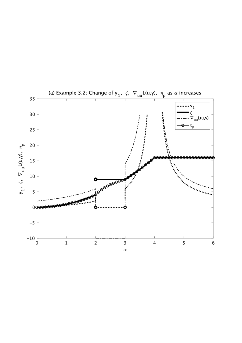
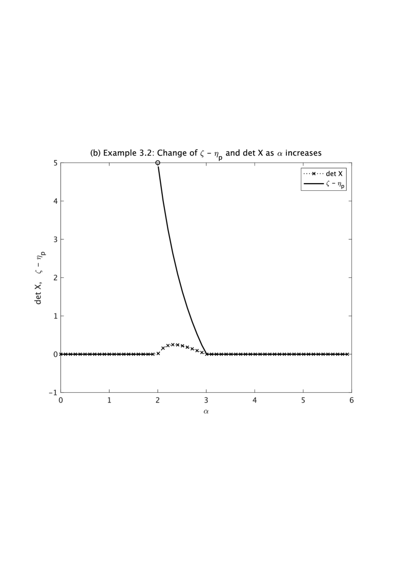
Figure 1: (a) Changes of $y_{1}$, $\nabla_{uu}$, $\zeta$ and $\eta_{p}$ as $\alpha$ increases from $2$ to $6$ in Example 3.2. (b) Changes of det$X$ and $\zeta-\eta_{p}$ as $\alpha$ increases from $2$ to $6$ in Example 3.2. Since $X_{11}=1$, det$X=0$ if and only if rank$X=1$.

Example 4.2.

$$\zeta = \inf\left\{q_{0}(\mbox{\boldmath$u$})\equiv 2u_{2}-2u_{1}:\begin{array}[]{l}q_{1}(\mbox{\boldmath$u$})\equiv-2u_{1}\leq 0,\ q_{2}(\mbox{\boldmath$u$})=-2u_{2}\leq 0,\\[2.0pt] q_{3}(\mbox{\boldmath$u$})\equiv u_{1}^{2}-u_{2}^{2}+1\leq 0\end{array}\right\},$$

where $n=2$ and $m=3$. This QCQP has a finite optimal value with no minimizer, and none of Conditions (A) through (F) hold. Obviously, every feasible $(u_{1},u_{2})$ satisfies $u_{1}\geq 0$ and $u_{2}\geq 1$. We also see that $-q_{3}(\mbox{\boldmath$u$})=(u_{2}-u_{1})(u_{2}+u_{1})-1\geq 0$, which implies that $u_{2}>u_{1}$ and $q_{0}(\mbox{\boldmath$u$})>0$ for every feasible solution $u$. Moreover, $\mbox{\boldmath$u$}=(u_{1},u_{2})=(u_{1},\sqrt{u_{1}^{2}+1})\in\mbox{$\mathbb{R}$}^{2}$ with $u_{1}\geq 0$ is a feasible solution with the objective value $q_{0}(\mbox{\boldmath$u$})=\sqrt{u_{1}^{2}+1}-u_{1}$, which tends to $0$ as $u_{1}\rightarrow\infty$. Hence $\zeta=0$ and there is no global minimizer. Letting

$$\left.\begin{array}[]{l}\mbox{\boldmath$Q$}_{0}=\begin{pmatrix}0&-1&1\\ -1&0&0\\ 1&0&0\end{pmatrix},\ \mbox{\boldmath$Q$}_{1}=\begin{pmatrix}0&-1&0\\ -1&0&0\\ 0&0&0\end{pmatrix},\\[3.0pt] \mbox{\boldmath$Q$}_{2}=\begin{pmatrix}0&0&-1\\ 0&0&0\\ -1&0&0\end{pmatrix},\ \mbox{\boldmath$Q$}_{3}=\begin{pmatrix}1&0&0\\ 0&1&0\\ 0&0&-1\end{pmatrix},\ \mbox{\boldmath$H$}=\begin{pmatrix}1&0&0\\ 0&0&0\\ 0&0&0\end{pmatrix},\end{array}\right\}$$ (60)

we obtain the primal SDP relaxation (27) and its dual (29). We can easily verify that if we take $u_{1}\geq 0$, then

$$\mbox{\boldmath$X$}=\begin{pmatrix}1&u_{1}&0\\ u_{1}&u_{1}^{2}&0\\ 0&0&u_{1}^{2}+1\end{pmatrix}$$

is a feasible solution of the primal SDP (27) with the objective $\mbox{\boldmath$Q$}_{0}\bullet\mbox{\boldmath$X$}=-2u_{1}$; hence $\eta_{p}=-\infty$. Therefore, the dual SDP (29) is infeasible. In fact, the constraints of the dual SDP (29) with $\mbox{\boldmath$Q$}_{k}$ $(0\leq k\leq 3)$ and $H$ given by (60) are written as

$$y_{k}\geq 0\ (k=1,2,3),$$

$$\mbox{\boldmath$S$}(\mbox{\boldmath$y$},s)\equiv\mbox{\boldmath$Q$}_{0}+\sum_{k=1}^{3}y_{k}\mbox{\boldmath$Q$}_{k}-s\mbox{\boldmath$H$}=\begin{pmatrix}y_{3}-s&-\frac{1}{2}-\frac{1}{2}y_{1}&\frac{1}{2}-\frac{1}{2}y_{2}\\ -\frac{1}{2}-\frac{1}{2}y_{1}&y_{3}&0\\ \frac{1}{2}-\frac{1}{2}y_{2}&0&-y_{3}\end{pmatrix}\in\mbox{$\mathbb{S}$}^{3}_{+}.$$

Clearly, there is no $(\mbox{\boldmath$y$},s)$ satisfying the constraints.

Example 4.3.

$$\zeta = \inf\left\{q_{0}(\mbox{\boldmath$u$})\equiv 2u_{2}-2u_{1}:\begin{array}[]{l}q_{1}(\mbox{\boldmath$u$})\equiv-2u_{1}\leq 0,\ q_{2}(\mbox{\boldmath$u$})=-2u_{2}\leq 0,\\[2.0pt] q_{3}(\mbox{\boldmath$u$})\equiv u_{1}^{2}-u_{2}^{2}+1\leq 0,\ q_{4}(\mbox{\boldmath$u$})\equiv 2u_{1}-2u_{2}\leq 0\end{array}\right\},$$

where $n=2$ and $m=4$. This QCQP is obtained by adding a redundant constraint $q_{4}(\mbox{\boldmath$u$})\leq 0$ to Example 4.2, so that its optimal value $\zeta$ remains as $0$ and it still has no minimizer. However, the characteristics of its SDP relaxation drastically changes. Defining

$$\mbox{\boldmath$Q$}_{4}=\begin{pmatrix}0&1&-1\\ 1&0&0\\ -1&0&0\end{pmatrix}\$$

in addition to $\mbox{\boldmath$Q$}_{k}\ (k=1,2,3)$ and $H$ given by(60), we obtain the primal SDP relaxation (27) and its dual (29). We can easily verify that

$$\mbox{\boldmath$X$}=\begin{pmatrix}1&0&0\\ 0&1&0\\ 0&0&2\end{pmatrix}$$

is a feasible solution of the primal SDP (27) with the objective $\mbox{\boldmath$Q$}_{0}\bullet\mbox{\boldmath$X$}=0$. We see that $(y_{1},y_{2},y_{3},y_{4},s)=(0,0,0,1,0)$ is a feasible solution of the dual SDP (29) with the objective value $0$. In fact,

$$\mbox{\boldmath$S$}(\mbox{\boldmath$y$},s) \equiv \mbox{\boldmath$Q$}_{0}+\sum_{k=1}^{4}y_{k}\mbox{\boldmath$Q$}_{k}-s\mbox{\boldmath$H$}$$

$$= \begin{pmatrix}y_{3}-s&-1-y_{1}+y_{4}&1-y_{2}-y_{4}\\ -1-y_{1}+y_{4}&y_{3}&0\\ 1-y_{2}-y_{4}&0&-y_{3}\end{pmatrix}=\mbox{\boldmath$O$}\in\mbox{$\mathbb{S}$}^{3}_{+}.$$

Hence, $\eta_{d}=\eta_{p}=\zeta=0$ and the KKT condition (32) holds. Thus, this example shows that even when the the KKT condition (32) and $\eta_{d}=\eta_{p}$ (the strong duality) hold, Condition ‘(D) $\eta_{p}=\zeta$’ does not necessarily ensure ‘Condition (C) primal SDP (27) is exact’ unless QCQP (1) has a minimizer.

Example 4.4.

$$\zeta = \inf\left\{q_{0}(\mbox{\boldmath$u$})\equiv u_{3}^{2}:\begin{array}[]{l}q_{1}(\mbox{\boldmath$u$})\equiv u_{1}^{2}\leq 0,\\[2.0pt] q_{2}(\mbox{\boldmath$u$})\equiv-2u_{1}u_{2}-2u_{3}^{2}+2\leq 0.\end{array}\right\},$$

where $n=3$ and $m=2$. This example illustrates a case where both Conditions (C) and (D) hold but Conditions (E) does not, even when QCQP (1) has a minimizer. Obviously, $(u_{1},u_{2},u_{3})=(0,0,1)$ is a minimizer with the objective value $\zeta=1$. Define

$$\left.\begin{array}[]{l}\mbox{\boldmath$Q$}_{0}=\begin{pmatrix}0&0&0&0\\ 0&0&0&0\\ 0&0&0&0\\ 0&0&0&1\end{pmatrix},\ \mbox{\boldmath$Q$}_{1}=\begin{pmatrix}0&0&0&0\\ 0&1&0&0\\ 0&0&0&0\\ 0&0&0&0\end{pmatrix},\\[3.0pt] \mbox{\boldmath$Q$}_{2}=\begin{pmatrix}2&0&0&0\\ 0&0&-1&0\\ 0&-1&0&0\\ 0&0&0&-2\end{pmatrix},\ \mbox{\boldmath$H$}=\begin{pmatrix}1&0&0&0\\ 0&0&0&0\\ 0&0&0&0\\ 0&0&0&0\end{pmatrix}.\end{array}\right\}$$ (65)

Then, we obtain the primal SDP relaxation (27) and its dual (29). It is easy to see that

$$\mbox{\boldmath$X$}=\begin{pmatrix}1&0&0&1\\ 0&0&0&0\\ 0&0&0&0\\ 1&0&0&1\end{pmatrix}$$

is a rank-$1$ feasible solution of the primal SDP (27) with the objective value $\eta_{p}=1=\zeta$; hence $X$ is an optimal solution of (27). On the other hand, the constraint of the dual SDP (29)

$$y_{1}\geq 0,\ y_{2}\geq 0,$$

$$\mbox{\boldmath$S$}(\mbox{\boldmath$y$},s)\equiv\mbox{\boldmath$Q$}_{0}+y_{1}\mbox{\boldmath$Q$}_{1}+y_{2}\mbox{\boldmath$Q$}_{2}-s\mbox{\boldmath$H$}\equiv\begin{pmatrix}2y_{2}-s&0&0&0\\ 0&y_{1}&-y_{2}&0\\ 0&-y_{2}&0&0\\ 0&0&0&1-2y_{2}\end{pmatrix}\in\mbox{$\mathbb{S}$}^{1+3}_{+}$$

holds if and only if $y_{1}\geq 0,y_{2}=0$ and $s\leq 0$. Hence, $(y_{1},y_{2},s)=(0,0,0)$ is an optimal solution of the dual SDP (29) with the optimal value $\eta_{d}=0$. Thus, $0=\eta_{d}<1=\eta_{p}=\zeta$ holds.

5 An extension of Conditions (B), (C), (D) and (E) to doubly nonnegative (DNN) relaxation

The SDP relaxation has played a major role in the discussion of Conditions (B), (C), (D) and (E). For QCQP in nonnegative variables, we can strengthen those conditions by replacing the SDP relaxation with a DNN relaxation. A lower bound provided by the DNN relaxation is known to be at least as tight as one by the SDP relaxation in theory and is often tighter in practice [14, 17].

To discuss conditions for the DNN relaxation, QCQP in nonnegative variables should be first described, for instance, by rewriting QCQP (1) as

$$\zeta = \inf\left\{q_{0}(\mbox{\boldmath$u$}^{+}-\mbox{\boldmath$u$}^{-}):\begin{array}[]{l}q_{k}(\mbox{\boldmath$u$}^{+}-\mbox{\boldmath$u$}^{-})+v_{k}=0\ (k\in M),\ v_{k}\geq 0\ (k\in M),\\[2.0pt] \mbox{\boldmath$u$}^{+}\geq\mbox{\bf 0},\ \mbox{\boldmath$u$}^{-}\geq 0,\ u^{+}_{i}u^{-}_{i}=0\ (1\leq i\leq n)\end{array}\right\},$$

where $\mbox{\boldmath$u$}^{+}\in\mbox{$\mathbb{R}$}^{n}$, $\mbox{\boldmath$u$}^{-}\in\mbox{$\mathbb{R}$}^{n}$ and $\mbox{\boldmath$v$}\in\mbox{$\mathbb{R}$}^{m}$ are nonnegative variables. From the transformed QCQP above, a DNN relaxation can be derived. The description of the resulting DNN relaxation would be very complicated. For simplicity of discussion, we instead consider a standard equality form QCQP:

$$\hat{\zeta} = \inf\left\{q_{0}(\mbox{\boldmath$u$}):q_{k}(\mbox{\boldmath$u$})=0\ (k\in M),\ \mbox{\boldmath$u$}\geq\mbox{\bf 0}\right\}.$$ (67)

Here $q_{k}:\mbox{$\mathbb{R}$}^{n}\rightarrow\mbox{$\mathbb{R}$}$ $(0\leq k\leq m)$ denote quadratic functions as used thus far.

Introducing redundant quadratic inequalities $u_{i}u_{j}\geq 0$ $(1\leq i,j\leq n)$, which can be represented as a matrix inequality $\begin{pmatrix}x_{0}^{2}&\mbox{\boldmath$u$}^{T}\\ \mbox{\boldmath$u$}&\mbox{\boldmath$u$}\mbox{\boldmath$u$}^{T}\end{pmatrix}\geq\mbox{\boldmath$O$}$ with $x_{0}^{2}=1$, and using the notation and symbols given in (23), we first transform QCQP (67) to the following QCQP:

$$\hat{\zeta} = \inf\left\{\mbox{\boldmath$Q$}_{0}\bullet\mbox{\boldmath$x$}\mbox{\boldmath$x$}^{T}:\mbox{\boldmath$x$}\mbox{\boldmath$x$}^{T}\geq\mbox{\boldmath$O$},\ \mbox{\boldmath$Q$}_{k}\bullet\mbox{\boldmath$x$}\mbox{\boldmath$x$}^{T}=0\ (k\in M),\ \mbox{\boldmath$H$}\bullet\mbox{\boldmath$x$}\mbox{\boldmath$x$}^{T}=1\right\}$$ (68)

$$= \inf\left\{\mbox{\boldmath$Q$}_{0}\bullet\mbox{\boldmath$x$}\mbox{\boldmath$x$}^{T}:\mbox{\boldmath$x$}\mbox{\boldmath$x$}^{T}\geq\mbox{\boldmath$O$},\ \mbox{\boldmath$x$}\mbox{\boldmath$x$}^{T}\in\widehat{F}\right\}.$$

Here $\widehat{F}=\left\{\mbox{\boldmath$X$}\in\mbox{$\mathbb{S}$}^{1+n}:\mbox{\boldmath$Q$}_{k}\bullet\mbox{\boldmath$x$}\mbox{\boldmath$x$}^{T}=0\ (k\in M),\ \mbox{\boldmath$H$}\bullet\mbox{\boldmath$x$}\mbox{\boldmath$x$}^{T}=1\right\}$. Replacing $\mbox{\boldmath$x$}\mbox{\boldmath$x$}^{T}$ with a matrix variable $\mbox{\boldmath$X$}\in\mbox{$\mathbb{S}$}^{1+n}_{+}$, we now obtain the primal SDP relaxation of QCQP(68) and its dual as follows.

$$\hat{\eta}_{p} = \inf\left\{\mbox{\boldmath$Q$}_{0}\bullet\mbox{\boldmath$X$}:\mbox{\boldmath$X$}\in\mbox{$\mathbb{S}$}^{1+n}_{+}\cap\mbox{$\mathbb{N}$},\ \mbox{\boldmath$X$}\in\widehat{\mbox{\boldmath$F$}}\right\},$$ (69)

$$\hat{\eta}_{d} = \sup\left\{s:\mbox{\boldmath$Q$}_{0}-\sum_{k\in M}y_{k}\mbox{\boldmath$Q$}_{k}-s\mbox{\boldmath$H$}\in\mbox{$\mathbb{S}$}^{1+n}_{+}+\mbox{$\mathbb{N}$},\ (\mbox{\boldmath$y$},s)\in\mbox{$\mathbb{R}$}^{m+1}\right\},$$ (70)

which serve as the primal DNN relaxation of QCQP (67) and its dual, respectively. Here $\mbox{$\mathbb{N}$}=\left\{\mbox{\boldmath$X$}\in\mbox{$\mathbb{S}$}^{1+n}:\mbox{\boldmath$X$}\geq\mbox{\boldmath$O$}\right\}$ (the cone of $(1+n)\times(1+n)$ nonnegative symmetric matrices). The Slater constraint qualification for the primal DNN (69) is written as

$$\left\{\mbox{\boldmath$X$}\in\widehat{F}:\mbox{\boldmath$X$}\in\mbox{$\mathbb{S}$}^{1+n}_{++},\ X_{ij}>0\ (1\leq i,j\leq n)\right\}\not=\emptyset.$$ (71)

Let $\widehat{G}=\mbox{$\mathbb{R}$}^{m+1}\times\mbox{$\mathbb{N}$}$. The Lagrangian function $L:\mbox{$\mathbb{R}$}^{n+m+1}\times\mbox{$\mathbb{S}$}^{1+n}\rightarrow\mbox{$\mathbb{R}$}$ for QCQP(68) is defined by

$$\widehat{L}(\mbox{\boldmath$x$},\mbox{\boldmath$y$},s,\mbox{\boldmath$Z$}) = \mbox{\boldmath$Q$}_{0}\bullet\mbox{\boldmath$x$}\mbox{\boldmath$x$}^{T}-\sum_{k\in M}y_{k}\mbox{\boldmath$Q$}_{k}\bullet\mbox{\boldmath$x$}\mbox{\boldmath$x$}^{T}-\mbox{\boldmath$Z$}\bullet\mbox{\boldmath$x$}\mbox{\boldmath$x$}^{T}-s(\mbox{\boldmath$H$}\bullet\mbox{\boldmath$x$}\mbox{\boldmath$x$}^{T}-1)$$

$$\mbox{for every }(\mbox{\boldmath$x$},\mbox{\boldmath$y$},s,\mbox{\boldmath$Z$})\in\mbox{$\mathbb{R}$}^{n+m+1}\times\mbox{$\mathbb{S}$}^{1+n}.$$

Hence, the saddle-point problem is: Find a $(\mbox{\boldmath$x$},\mbox{\boldmath$y$},s,\mbox{\boldmath$Z$})\in\mbox{$\mathbb{R}$}^{1+n}\times\widehat{G}$ such that

$$\sup_{(\mbox{\boldmath$y$}^{\prime},s^{\prime},\mbox{\boldmath$Z$}^{\prime})\in\widehat{G}}L(\mbox{\boldmath$x$},\mbox{\boldmath$y$}^{\prime},s^{\prime},\mbox{\boldmath$Z$}^{\prime})=L(\mbox{\boldmath$x$},\mbox{\boldmath$y$},s,\mbox{\boldmath$Z$})=\inf_{\mbox{\boldmath$x$}^{\prime}\in\mbox{$\mathbb{R}$}^{n}}L(\mbox{\boldmath$x$}^{\prime},\mbox{\boldmath$y$},s,\mbox{\boldmath$Z$}),$$

and the Lagrangian dual is:

$$\hat{\varphi} = \sup_{(\mbox{\boldmath$y$},s,\mbox{\boldmath$Z$})\in\widehat{G}}\ \inf_{\mbox{\boldmath$x$}\in\mbox{$\mathbb{R}$}^{n}}L(\mbox{\boldmath$x$},\mbox{\boldmath$y$},s,\mbox{\boldmath$Z$}).$$

We are now ready to present the following relations.

$$\left.\begin{array}[]{lcl}&&\mbox{($\widehat{\rm A}$) $\exists$ a saddle point $(\mbox{\boldmath$x$},\mbox{\boldmath$y$},s,\mbox{\boldmath$Z$})$ of the Lagrangian function $\widehat{L}$}.\\[2.0pt] &&\Updownarrow\\[2.0pt] &&\mbox{($\widehat{\rm B}$) the primal DNN~{}\eqref{eq:PDNN} is exact},\\[2.0pt] &&\hskip 17.07164pt\mbox{$\exists$ an optimal solution $(\mbox{\boldmath$y$},s,\mbox{\boldmath$Z$})$ of the dual DNN~{}\eqref{eq:DDNN} and}\\[2.0pt] &&\hskip 17.07164pt\mbox{$\hat{\eta}_{d}=\hat{\eta}_{p}$ (the strong duality)}.\\[2.0pt] &&\Downarrow\hskip 2.84526pt\Uparrow\mbox{if ($\hat{\rm a}$) the Slater constraint qualification~{}\eqref{eq:Slater2} holds.}\\[2.0pt] &&\mbox{($\widehat{\rm C}$) the primal DNN~{}\eqref{eq:PDNN} is exact.}\\[2.0pt] &&\Downarrow\hskip 5.69054pt\Uparrow\mbox{if ($\hat{\rm b}$) QCQP~{}\eqref{eq:QCQP02} has a minimizer $\mbox{\boldmath$x$}$ when $\hat{\zeta}$ is finite.}\\[2.0pt] &&\mbox{($\widehat{\rm D}$) $-\infty<\hat{\eta}_{p}=\hat{\zeta}<\infty$.}\\[2.0pt] &\mbox{if ($\widehat{\rm B}$) holds}&\Downarrow\hskip 8.53581pt\Uparrow\\[2.0pt] &&\mbox{($\widehat{\rm E}$) $-\infty<\hat{\eta}_{d}=\hat{\zeta}<\infty$}\Longleftrightarrow\mbox{($\widehat{\rm F}$) $-\infty<\hat{\varphi}=\hat{\zeta}<\infty$.}\end{array}\right\}$$ (83)

We can prove these relations similarly as in Section 3. The details are omitted.

6 Concluding remarks

When QCQP (1) has a finite optimal value, the following two cases, (a) and (b), can be considered: (a) the Slater constraint qualification (36) holds, (b) QCQP (1) has a minimizer, If (a) and (b) are satisfied, then Conditions (A) through (F) for global optimality of QCQP (1) are all equivalent. It was shown in [8] that (a) is a generic property of conic optimization problems. Also, if the feasible region of QCQP (1) is bounded, then (b) holds. Therefore (a) and (b) may be regarded as moderate assumptions to avoid special degenerate cases.

For (a), however, we should be more carful as it may be frequently violated in practice. Moreover, judging numerically whether (a) is satisfied or not is not an easy task in practice. Many computational methods including interior-point methods for solving SDPs assume (a) for their convergence analysis, and often encounter the numerical difficulty when (a) is not satisfied.

Statements and Declarations

The authors declare that they have no competing interests.

References

• [1] G. Azuma, M. Fukuda, S. Kim, and M. Yamashita. Exact SDP relaxations of quadratically constrained quadratic programs with bipartite graph structures. Journal of Global Optimization, https://doi.org/10.1007/s10898-022-01268-3, 2022.
• [2] G. Azuma, M. Fukuda, S. Kim, and M. Yamashita. Exact SDP relaxations of quadratically constrained quadratic programs with forest structures. Journal of Global Optimization, 82(2):243–262, 2022.
• [3] N. V. Bao, X. Sahinidis and M. Tawarmalani. Semidefinite relaxations for quadratically constrained quadratic programming: A review and comparisons. Mathematical Programming, 129:129–157, 2011.
• [4] M. S. Bazaraa, H. D. Sherali, and Shetty C. M. Nonlinear Programming: Theory and Algorithms. John Wiley and Sons, Hoboken, NJ, 2006.
• [5] S. Burer. On the copositive representation of binary and continuous non-convex quadratic programs. Mathematical Programming, 120:479–495, 2009.
• [6] S. Burer and Y. Ye. Exact semidefinite formulations for a class of (random and non-random) nonconvex quadratic programs. Mathematical Programming, 181:1–17, 2020.
• [7] E. de Klerk and D. V. Pasechnik. Approximation of the stability number of a graph via copositive programming. SIAM Jornal on Optimization, 12(875-892), 2002.
• [8] M. Dür, B. Jargalsaikhan, and G. Still. Genericity results in linear conic programming—a tour dh́orizon. Mathematics of Operations Research, 42(1):77–94, 2017.
• [9] M Dür and F. Rendle. Conic optimization: a survey with special focus on copositive optimization and binary quadratic problems. EURO Journal of Operational Research, 9, 2021.
• [10] T. Fujie and M. Kojima. Semidefinite programming relaxation for nonconvex quadratic programs. Journal of Global Optimization, 10:367–368, 1997.
• [11] M. X. Goemans and D. P. Williamson. Improved approximation algorithms for maximum cut and satisfiability problems using semidefinite programming. Journal of the ACM, 42(6):1115–1145, 1995.
• [12] V. Jeyakumar and G. Y. Li. Trust-region problems with linear inequality constraints: Exact SDP relaxation, global optimality and robust optimization. Mathematical Programming, 147(1-2):171–206, 2014.
• [13] S. Kim and M. Kojima. Exact solutions of some nonconvex quadratic optimization problems via SDP and SOCP relaxations. Computational Optimization and Applications, 26:143–154, 2003.
• [14] S. Kim, M. Kojima, and K. C. Toh. A Lagrangian-DNN relaxation: a fast method for computing tight lower bounds for a class of quadratic optimization problems. Mathematical Programming, 156:161–187, 2016.
• [15] S. Kim, M. Kojima, and K. C. Toh. Doubly nonnegative relaxations are equivalent to completely positive reformulations of quadratic optimization problems with block-clique graph structures. Journal of Global Optimization, 77(3):513–541, 2020.
• [16] S. Kim, M. Kojima, and K. C. Toh. A geometric analysis of a class of nonconvex conic programs for convex conic reformulations of quadratic and polynomial optimization problems. SIAM Journal on Optimization, 30:1251–1273, 2020.
• [17] S. Kim, M. Kojima, and K. C. Toh. A Newton-bracketing method for a simple conic optimization problem. Optimization Methods and Software, 36:371–388, 2021.
• [18] Loiola E. M., de Abreu N.M.M., Boaventura-Netto P.O., Hahn P., and Querido T. A survey for the quadratic assignment problem. European Journal of Operational Research, 176:657–690, 2007.
• [19] C. Lu, S-C. Fang, Q. Jin, Z. Wang, and W. Xing. KKT solution and conic relaxation for solving quadratically constrained quadratic programming problems. SIAM Journal on Optimization, 21(4):1475–1490, 2011.
• [20] O.L. Mangasarian. Nonlinear Programming, volume McGraw-Hill Book Company. 1969.
• [21] M. Mevissen and M. Kojima. SDP relaxations for quadratic optimization problems derived from polynomial optimization problems. Asia-Pacific Journal of Operational Research, 27(1):15–38, 2010.
• [22] J. Povh and F. Rendl. A copositive programming approach to graph partitioning. SIAM Journal on Optimization, 18:223–241, 2007.
• [23] N. Z. Shor. Quadratic optimization problems. Soviet Journal of Computer and Systems Sciences, 25:1–11, 1987.
• [24] N. Z. Shor. Dual quadratic estimates in polynomial and boolean programming. Annals of Operations Research, 25:163–168, 1990.
• [25] S. Sojoudi and J. Lavaei. Exactness of semidefinite relaxations for nonlinear optimization problems with underlying graph structure. SIAM Journal on Optimization, 24:1746–1778, 2014.
• [26] Alex L. Wang and Fatma K$i$l$i$nç-Karzan. On the tightness of SDP relaxations of QCQPs. Mathematical Programming, 2021.
• [27] A. Yoshise and Y. Matsukawa. On optimization over the doubly nonnegative cone. IEEE Multi-conference on Systems and Control, 2010.
• [28] S. Zhang. Quadratic optimization and semidefinite relaxation. Mathematical Programming, 87(453-465), 2000.