ANITA: Analytic Tableau Proof Assistant

Abstract

This work presents the system ANITA (Analytic Tableau Proof Assistant) developed for teaching analytic tableaux to computer science students. The tool is written in Python and can be used as a desktop application, or in a web platform. This paper describes the logical system of the tool, explains how the tool is used and compares it to several similar tools. ANITA has already been used in logic courses and an evaluation of the tool is presented.

1 Introduction

Logic in Computer Science course is part of most Information and Communication Technology curricula, such as the curricula of the Information Systems, Software Engineering, Computer Science, and Computer Engineering of the Federal University of Ceará at Quixadá as mandatory components. The course has a high failure rate. For better assimilation of the contents, it is essential that the students exercise and that they get feedback on the correctness of their proofs.

Many deductive systems are used for teaching the formal reasoning of proofs, such as Axiomatic Systems (a la Hilbert), Natural Deduction System [8, 9], and Analytic Tableaux [13, 3].

The Analytic Tableau system is widely used for teaching proofs and appears in many Logic textbooks such as [13, 12, 14, 5]. This work presents a proof assistant, ANITA (Analytic Tableau Proof Assistant), in order to assist in the teaching-learning of undergraduate and graduate students. For the purpose of teaching deduction systems, we take into account in ANITA the following features: the students should write their proofs as similar as possible to what is available in the textbooks and to what the students would usually write on paper; the tool should be easy-to-use and reduce the number of clicks since mouse-clicking can be tedious; the tool should allow the student to make mistakes and point out errors on the proofs.

The rest of the paper is organized as follows. We provide a concise definition of Analytic Tableau system in Section 2; We propose to write proofs in Analytic Tableaux in Fitch-style in Section 3. Section 4 describes ANITA. Section 5 compares ANITA to other proof assistants. The evaluation of ANITA is presented in Section 6. And, we conclude this work in Section 7.

2 Analytic Tableaux

We now describe Analytic Tableaux for propositional logic which we will subsequently extend to first-order logic.

Analytic Tableaux is an inference method based on refutation: to prove $\Gamma\vdash\varphi$, we assert that each formula of $\Gamma$ is true and $\varphi$ is false, in order to derive a contradiction. On the other hand, if no contradiction is obtained, then we construct a countermodel, that is, a valuation that satisfies $\Gamma$ and does not satisfy $\varphi$.

In the method of analytic tableaux, we define $T~{}\varphi$ and $F~{}\varphi$ as signed formulas to stand that $\varphi$ is true and $\varphi$ is false. The first step to constructing a tableau is to label all formulas in $\Gamma$ with $T$ and the formula $\varphi$ with $F$. Starting from the initial tableau, tableau expansion rules can be used to: add new formulas to the end of a branch ($\alpha$-type rules); or split a branch into two branches ($\beta$-type rules). The rules for the construction of tableaux are as follows:

$\alpha$ rule	[. $T~{}\varphi\wedge\psi$ [. $T~{}\varphi$
$T~{}\psi$ ] ]	[. $F~{}\varphi\vee\psi$ [. $F~{}\varphi$
$F~{}\psi$ ] ]	[. $F~{}\varphi\rightarrow\psi$ [. $T~{}\varphi$
$F~{}\psi$ ] ]	[. $T~{}\lnot\varphi$ [. $F~{}\varphi$ ] ]	[. $F~{}\lnot\varphi$ [. $T~{}\varphi$ ] ]
$\beta$ rule	[. $F~{}\varphi\wedge\psi$ [. $F~{}\varphi$ ] [. $F~{}\psi$ ] ]	[. $T~{}\varphi\vee\psi$ [. $T~{}\varphi$ ] [. $T~{}\psi$ ] ]	[. $T~{}\varphi\rightarrow\psi$ [. $F~{}\varphi$ ] [. $T~{}\psi$ ] ]

In each branch, a formula can only be expanded once. A branch that has no more formulas to expand is said to be saturated. A branch that has a pair of formulas $T~{}\varphi$ and $F~{}\varphi$ is said to be closed. A closed branch no longer needs to be expanded. A tableau is said to be closed whether it has all its branches closed, i.e., $\Gamma\vdash\varphi$. A saturated and unclosed branch provides a countermodel, i.e., $\Gamma\not\vdash\varphi$. Figure 1(a) shows that $A\rightarrow B,B\rightarrow C,A$ entails $C$ as an analytic tableau proof. We use $\times$ as a symbol to close a branch by the signed formulas in the blue nodes. Figure 1(b) shows a proof, in which we have one of the branches (red nodes) that is saturated. So, we can extract a countermodel from the truth values of the atoms in the branch.

[.$T~{}A\rightarrow B$
$T~{}B\rightarrow C$
$T~{}A$
$F~{}C$ [.$F~{}A$ [.$\times$ ] ] [.$T~{}B$ [.$F~{}B$ [.$\times$ ] ] [.$T~{}C$ [.$\times$ ] ] ] ]

(a) $A\rightarrow B,B\rightarrow C,A\vdash C$

[.$T~{}A$
$T~{}(A\land B)\rightarrow C$
$F~{}C$ [.$F~{}A\land B$ [.$F~{}A$ [.$\times$ ] ] [.$F~{}B$ ] ] [.$T~{}C$ [.$\times$ ] ] ]
Countermodel:
$v(A)=T$ and $v(B)=v(C)=F$

(b) $A,A\wedge B\rightarrow C\not\vdash C$

Figure 1: Examples of proofs in Analytic Tableau

We extend the analytic tableau system in order to include proofs of first-order logic, in which we have all the rules of propositional logic and add the following rules:

$\gamma$ rule	[. $T~{}\forall x\varphi$ [. $T~{}\varphi^{x}_{t}$ ] ]	[. $F~{}\exists x\varphi$ [. $F~{}\varphi^{x}_{t}$ ] ]
	$t$ is substitutable for $x$ in $\varphi$	$t$ is substitutable for $x$ in $\varphi$
$\delta$ rule	[. $F~{}\forall x\varphi$ [. $F~{}\varphi^{x}_{a}$ ] ]	[. $T~{}\exists x\varphi$ [. $T~{}\varphi^{x}_{a}$ ] ]
	a is a new variable	a is a new variable

Here $\varphi^{x}_{t}$ is the expression obtained from the formula $\varphi$ by replacing the variable $x$, whenever it occurs free in $\varphi$, by the term $t$. For instance, $(H(x)\rightarrow\forall xM(x))^{x}_{y}=(H(y)\rightarrow\forall xM(x))$. We can say that a term $t$ is substitutable for $x$ in $\varphi$ if there is no variable $y$ in $t$ that is captured by a $\forall y$ (or $\exists y$) quantifier of $\varphi^{x}_{t}$. For example, term $z$ is substitutable for $y$ in $\forall xP(x,y)$. On the other hand, term $x$ is not substitutable for $y$ in $\forall xP(x,y)$.

The above rules can occur more than once in each branch, as we can make arbitrary substitutions of variables. Thus, in the general case, we will not be able to generate a countermodel. Figure 2 shows examples of proofs in Analytic Tableaux.

[.$T~{}\forall x(H(x)\rightarrow M(x))$
$T~{}\forall xH(x)$
$F~{}\forall xM(x)$ [.$F~{}M(a)$ [.$T~{}H(a)\rightarrow M(a)$ [.$T~{}H(a)$ [.$F~{}H(a)$ [.$\times$ ] ] [.$T~{}M(a)$ [.$\times$ ] ] ] ] ] ]

(a) $\forall x(H(x)\rightarrow M(x)),\forall xH(x)\vdash\forall xM(x)$

[.$T~{}\forall x(H(x)\rightarrow M(x))$
$T~{}\exists xH(x)$
$F~{}\exists xM(x)$ [.$T~{}H(a)$ [.$F~{}M(a)$ [.$T~{}H(a)\rightarrow M(a)$ [.$F~{}H(a)$ [.$\times$ ] ] [.$T~{}M(a)$ [.$\times$ ] ] ] ] ] ]

(b) $\forall x(H(x)\rightarrow M(x)),\exists xH(x)\vdash\exists xM(x)$

Figure 2: Examples of Proofs in Analytic Tableaux

3 Analytic Tableaux in Fitch-Style

A (signed) tableau is a certain kind of binary, labeled ordered tree where each node is labeled by a signed formula. However, we can present a version of the analytic tableaux in Fitch-style. The proof is written in a linear and sequential order, in which we number all the lines, and write a statement (signed formula) with its justification which can be a premise, the conclusion of the proof, or the application of one of the inference rules. Each split of a branch is delimited by $\{$ and $\}$. A formula can only be used in a proof at a given point if that formula happened previously and within that branch. In the sequel, we will present all the rules in Fitch-style.

Initial Tableau Rule:

A proof of $\varphi_{1},\varphi_{2},\ldots,\varphi_{n}\vdash\psi$ starts with initial tableau as shown in Figure 3(a), where:

• The premises $\varphi_{1},\varphi_{2},\ldots,\varphi_{n}$ are represented in one line each, following a sequential numbering, labeled as $T$ (True) and as justification “Premise”.

• The conclusion $\psi$ is defined on the line after the last premise, labeled by $F$ (False) and with the justification “Conclusion”.

1.	$~{}T~{}\varphi_{1}$	Premise
2.	$~{}T~{}\varphi_{2}$	Premise
$\vdots$	$\vdots$	$\vdots$
n.	$~{}T~{}\varphi_{n}$	Premise
n+1.	$~{}F~{}\psi$	Conclusion
$\vdots$	$\vdots$	$\vdots$

(a) Initial Tableau

2 T A & Premise
F A Conclusion
⋮ ⋮

(b) Sample $A\vdash A$

Figure 3: Initial Tableau Rule

Closed Branch Rule:

We say that a branch is closed (contains a contradiction $\bot$) in line $p$ if a formula $\varphi$ is labeled in one line $m$ with $T$ and in another line $n$ with $F$ (both before $p$). A closed branch can no longer be expanded. Figure 4(a) presents the scheme of this rule. Figure 4(b) shows the proof of $A\vdash A$, in which we close the (single) branch in line $3$ from the formula $A$ referenced in lines $1$ and $2$ as $T$ and $F$, respectively.

⋮	⋮	⋮
$m$.	$~{}T~{}\varphi$
⋮	⋮	⋮
$n$.	$~{}F~{}\varphi$
⋮	⋮	⋮
$p$.	$\bot$	$m$,$n$

(a) Closed Branch

2 T A & Premise
F A Conclusion
⊥ 1,2

(b) $A\vdash A$

Figure 4: Closed Branch Rule

The negation-true rule ($\lnot T$) is shown in Figure 5(a), where the signed formula $F~{}\varphi$ can be obtained in line $n$ by the signed formula $T~{}\lnot\varphi$ in line $m$. In a similar way, the negation-false rule ($\lnot F$), see Figure 5(b), can be used to show $T~{}\varphi$ in line $n$ by $F~{}\lnot\varphi$ in line $m$. As we can see, in Figure 5(c), we conclude $T~{}\lnot A$ in line $3$ by the negation-false rule in line $2$. So, we apply $\lnot T$ rule and get $F~{}A$ in line $4$. Thus, we close the branch in line $5$ (a contradiction), because we have $T~{}A$ in line $1$ and $F~{}A$ in line $4$.

⋮	⋮	⋮
m.	$~{}T~{}\lnot\varphi$
⋮	⋮	⋮
n.	$~{}F~{}\varphi$	$m$

(a) Negation-True ($\lnot T$)

⋮	⋮	⋮
m.	$~{}F~{}\lnot\varphi$
⋮	⋮	⋮
n.	$~{}T~{}\varphi$	$m$

(b) Negation-False ($\lnot F$)

2 T A & Premise
F ¬¬A Conclusion
T ¬A 2
F A 3
⊥ 1,4

(c) $A\vdash\lnot\lnot A$

Figure 5: Negation Rules

The and-true rule ($\land T$) is shown in Figure 6(a), in which the signed formulas $T~{}\varphi$ and $T~{}\psi$ in lines $n$ and $n+1$, respectively, are obtained by the signed formula $T~{}\varphi\land\psi$ in line $m$. For example, in Figure 6(b), we apply rule $\land T$ to $T~{}A\land B$ in line $1$ and derive $T~{}A$ and $T~{}B$, in lines $3$ and $4$.

⋮	⋮	⋮
m.	$~{}T~{}\varphi\land\psi$
⋮	⋮	⋮
n.	$~{}T~{}\varphi$	$m$
n+1.	$~{}T~{}\psi$	$m$

(a) And-True ($\land T$)

2 T A∧B & Premise
F A Conclusion
T A 1
T B 1
⊥ 2,3

(b) $A\land B\vdash A$

Figure 6: And-True Rule

The and-false rule ($\land F$) is shown in Figure 7(a). This rule is applied to $F~{}\varphi\land\psi$ in line $m$ and splits this branch into two: one that starts in line $n$ with $F~{}\varphi$; and the other in line $p$ with $F~{}\psi$. To delimit the respective branches, we use the symbols $\{$ and $\}$. For instance, in Figure 7(b), we apply $\land F$ rule to $F~{}A\wedge B$ in line $3$ and split this branch:

1. In the branch starting in line $4$ with $F~{}A$ which is used with $T~{}A$ from line $1$ to close this branch in line $5$.

2. In the branch starting in line $6$ with $F~{}B$ which is used with $T~{}B$ from line $2$ to close this branch in line $7$.

It is worth noting that we can only reference the formulas in the same branch. So, for example, the formula $F~{}A$ in line $4$ could not be referenced in the branch starting in line $6$.

⋮	⋮	⋮
m.	$~{}F~{}\varphi\land\psi$
⋮	⋮	⋮
n.	{  $F~{}\varphi$	$m$
⋮	⋮	⋮
	}
p.	{  $F~{}\psi$	$m$
⋮	⋮	⋮
	}

(a) And-False ($\land F$)

2 T A & Premise
T B Premise
F A∧B Conclusion
{  F A 3
   ⊥ 1,4$~{}~{}\}$
{  F B 3
   ⊥ 2,6$~{}~{}\}$

(b) $A,B\vdash A\land B$

Figure 7: And-False Rule

The or-true rule ($\lor T$) is presented in Figure 8(a). We apply this rule to $T~{}\varphi\lor\psi$ in line $m$ and we split this branch into two new branches: one that starts in line $n$ with $T~{}\varphi$; and the other in line $p$ with $T~{}\psi$. For example, in Figure 8(b), the rule $\lor T$ is applied to $T~{}A\lor B$ in line $1$ and we split this branch:

1. In the branch that starts in line $5$ with $T~{}A$ which is used with $F~{}A$ in line $3$ to close this branch in line $6$.

2. In the branch starting in line $7$ with $T~{}B$ which is used with $F~{}B$ in line $4$ to close this branch in line $8$.

⋮	⋮	⋮
m.	$~{}T~{}\varphi\lor\psi$
⋮	⋮	⋮
n.	{  $T~{}\varphi$	$m$
⋮	⋮	⋮
	}
p.	{  $T~{}\psi$	$m$
⋮	⋮	⋮
	}

(a) Or-True ($\lor T$)

2 T A∨B & Premise
T ¬B Premise
F A Conclusion
F B 2
{  T A 1
   ⊥ 3,5$~{}~{}\}$
{  T B 1
   ⊥ 4,7$~{}~{}\}$

(b) $A\lor B,\lnot B\vdash A$

Figure 8: Or-True Rule

The or-false rule ($\lor F$) is shown in Figure 9(a), in which the signed formulas $F~{}\varphi$ and $F~{}\psi$ in lines $n$ and $n+1$, respectively, are obtained by the signed formula $F~{}\varphi\lor\psi$. For example, in Figure 9(b), we apply rule $\lor F$ to $F~{}A\lor B$ in line $2$ and derive $F~{}A$ and $F~{}B$, in lines $3$ and $4$.

⋮	⋮	⋮
m.	$~{}F~{}\varphi\lor\psi$
⋮	⋮	⋮
n.	$~{}F~{}\varphi$	$m$
n+1.	$~{}F~{}\psi$	$m$

(a) Or-False ($\lor F$)

2 T A & Premise
F A∨B Conclusion
F A 2
F B 2
⊥ 1,3

(b) $A\vdash A\lor B$

Figure 9: Or-False Rule

The implication-true rule ($\rightarrow T$) is presented in Figure 10(a). We apply this rule to $T~{}\varphi\rightarrow\psi$ in line $m$ and we split this branch into two new branches: one that starts in line $n$ with $F~{}\varphi$; and the other in line $p$ with $T~{}\psi$. For example, in Figure 10(b), the rule $\rightarrow T$ is applied to $T~{}A\rightarrow B$ in line $1$ and we split this branch:

1. In the branch that starts in line $5$ with $F~{}\lnot A$, in which we apply $\lnot F$ to obtain $T~{}A$ in line $6$ and, then, we use $F~{}A$ in line $3$ to close this branch in line $7$.

2. In the branch starting in line $8$ with $T~{}B$ which is used with $F~{}B$ in line $4$ to close this branch in line $9$.

⋮	⋮	⋮
m.	$~{}T~{}\varphi\rightarrow\psi$
⋮	⋮	⋮
n.	{  $F~{}\varphi$	$m$
⋮	⋮	⋮
	}
p.	{  $T~{}\psi$	$m$
⋮	⋮	⋮
	}

(a) Implication-True ($\rightarrow T$)

2 T ¬A→B & Premise
F A∨B Conclusion
F A 2
F B 2
{  F ¬A 1
   T A 5
   ⊥ 6,3$~{}~{}\}$
{  T B 1
   ⊥ 8,4$~{}~{}\}$

(b) $\lnot A\rightarrow B\vdash A\lor B$

Figure 10: Implication-True Rule

The implication-false rule ($\rightarrow F$) is shown in Figure 11(a), in which the signed formulas $T~{}\varphi$ and $F~{}\psi$ in lines $n$ and $n+1$, respectively, are obtained by the signed formula $F~{}\varphi\rightarrow\psi$. For example, in Figure 11(b), we apply rule $\rightarrow F$ to $F~{}A\rightarrow B$ in line $2$ and derive $T~{}A$ and $F~{}B$, in lines $3$ and $4$.

⋮	⋮	⋮
m.	$~{}F~{}\varphi\rightarrow\psi$
⋮	⋮	⋮
n.	$~{}T~{}\varphi$	$m$
n+1.	$~{}F~{}\psi$	$m$

(a) Implication-False ($\rightarrow F$)

2 T B & Premise
F A→B Conclusion
T A 2
F B 2
⊥ 1,4

(b) $B\vdash A\rightarrow B$

Figure 11: Implication-False Rule

The universal-true rule ($\forall T$) is shown in Figure 12(a), in which we apply $\forall T$-rule to signed formula $T~{}\forall x\varphi(x)$ in line $m$ and obtain, in line $n$, a signed formula $T~{}\varphi^{x}_{t}$, where $t$ is substitutable for $x$ in $\varphi$. Figure 12(b) shows the use of this rule to $T~{}\forall x(H(x)\rightarrow M(x))$ in line $1$ to get $T~{}H(s)\rightarrow M(s)$ in line $4$.

⋮	⋮	⋮
m.	$~{}T~{}\forall x\varphi$
⋮	⋮	⋮
n.	$~{}T~{}\varphi^{x}_{t}$	$m$

$t$ is substitutable for $x$ in $\varphi$

(a) Universal-True ($\forall T$)

2 T ∀x(H(x) →M(x)) & Premise
T H(s) Premise
F M(s) Conclusion
T H(s) →M(s) 1
{  F H(s) 4
   ⊥ 2,5$~{}~{}\}$
{  T M(s) 4
   ⊥ 7,3$~{}~{}\}$

(b) $\forall x(H(x)\rightarrow M(x)),H(s)\vdash M(s)$

Figure 12: Universal-True Rule

The universal-false rule ($\forall F$) is shown in Figure 13(a), in which we apply $\forall F$-rule to signed formula $F~{}\forall x\varphi(x)$ in line $m$ and obtain, in line $n$, a signed formula $F~{}\varphi^{x}_{a}$, where $a$ is a new variable. Figure 13(b) illustrates the use of this rule to $F~{}\forall xM(x)$ in line $3$ to conclude $F~{}M(a)$ in line $4$.

⋮	⋮	⋮
m.	$~{}F~{}\forall x\varphi$
⋮	⋮	⋮
n.	$~{}F~{}\varphi^{x}_{a}$	$m$

$a$ is new variable

(a) Universal-False ($\forall F$)

2 T ∀x(H(x) →M(x)) & Premise
T ∀x H(x) Premise
F ∀x M(x) Conclusion
F M(a) 3
T H(a) 2
T H(a) →M(a) 1
{  F H(a) 6
   ⊥ 5,7$~{}~{}\}$
{  T M(a) 6
   ⊥ 9,4$~{}~{}\}$

(b) $\forall x(H(x)\rightarrow M(x)),\forall xH(x)\vdash\forall xM(x)$

Figure 13: Universal-False Rule

The existential-true rule ($\exists T$) is shown in Figure 14(a), in which we apply $\exists T$-rule to signed formula $T~{}\exists x\varphi(x)$ in line $m$ and obtain, in line $n$, a signed formula $T~{}\varphi^{x}_{a}$, where $a$ is a new variable. Figure 14(b) illustrates the use of this rule to $T~{}\exists x~{}H(x)$ in line $2$ to get $T~{}H(a)$ in line $4$.

⋮	⋮	⋮
m.	$~{}T~{}\exists x\varphi$
⋮	⋮	⋮
n.	$~{}T~{}\varphi^{x}_{a}$	$m$

$a$ is new variable

(a) Existential-True ($\exists T$)

2 T ∀x(H(x) →M(x)) & Premise
T ∃x H(x) Premise
F  ∃x M(x) Conclusion
T H(a) 2
F M(a) 3
T H(a) →M(a) 1
{  F H(a) 6
   ⊥ 4,7$~{}~{}\}$
{  T M(a) 6
   ⊥ 5,9$~{}~{}\}$

(b) $\forall x(H(x)\rightarrow M(x)),\exists xH(x)\vdash\exists xM(x)$

Figure 14: Existential-True Rule

The existential-false rule ($\exists F$) is shown in Figure 15(a), in which we apply $\exists F$-rule to signed formula $F~{}\exists x\varphi(x)$ in line $m$ and obtain, in line $n$, a signed formula $F~{}\varphi^{x}_{t}$, where $t$ is substitutable for $x$ in $\varphi$. Figure 15(b) illustrates the use of this rule to $F~{}\exists xP(x)$ in line $4$ to conclude $P(a)$ in line $5$.

⋮	⋮	⋮
m.	$~{}F~{}\exists x\varphi$
⋮	⋮	⋮
n.	$~{}F~{}\varphi^{x}_{t}$	$m$

$t$ is substitutable for $x$ in $\varphi$

(a) Existential-False ($\exists F$)

2 T P(a) & Premise
T ∃x P(x) →B Premise
F  B Conclusion
{  F ∃x P(x) 2
   F P(a) 4
   ⊥ 1,5$~{}~{}\}$
{  T B 2
   ⊥ 7,3$~{}~{}\}$

(b) $P(a),\exists xP(x)\rightarrow B\vdash B$

Figure 15: Existential-False Rule

4 Analytic Tableau Proof Assistant (ANITA)

The ANITA proof assistant, Analytic Tableau Proof Assistant, is a tool written in Python that can be used as a desktop application, or in a web platform. The main idea is that the students can write their proofs as similar as possible to what is available in the textbooks and to what the students would usually write on paper. ANITA allows the students to automatically check whether a proof in the analytic tableaux is valid. If the proof is not correct, the tool will display the errors on the proof. So, the students may make mistakes and learn from the errors. The web interface is very easy-to-use and has:

• An area for editing the proof in plain text. The students should write a proof in Fitch-style presented in Section 3.

• A message area to display whether the proof is valid, the countermodel, or the errors on the proof.

• And the following links: Check, to check the correctness of the proof; Manual, to view a document with the inference rules and examples; LaTeX, to generate the LaTeX code of the trees from a valid proof; Latex in Overleaf to open the proof source code directly in Overleaf.

To facilitate the writing of the proofs, we made the following conventions in ANITA:

• The Atoms are written in capital letters (e.g. A, B, H(x));

• Variables are written with the first letter in lowercase, followed by letters and numbers (e.g. x, x0);

• Formulas with $\forall x$ and $\exists x$ are represented by $Ax$ and $Ex$ (‘A’ and ‘E’ followed by the variable x). For instance, Ax (H(x)$-\!\!>$M(x)) represents $\forall x~{}(H(x)\rightarrow M(x))$.

• Figure 16 shows the equivalence of logic symbols and those used in ANITA.

• The order of precedence of quantifiers and logical connectives is defined by $\lnot,\forall,\exists,\wedge,\vee,\rightarrow$ with right alignment. For example:

  • Formula $\sim$A&B$-\!\!>$C represents formula $(((\lnot A)\land B)\rightarrow C)$;

  • The theorem $\sim$A$\mid$B $|-$ A$-\!\!>$C represents $((\lnot A)\vee B)\vdash(A\rightarrow C)$.

• Each inference rule will be named by its respective connective and the truth value of the signed formula. For example, &T represents the and-true rule. Optionally, the rule name can be omitted.

• The justifications for the premises and the conclusion use the reserved words pre and conclusion, respectively.

Symbol	$\lnot$	$\land$	$\lor$	$\rightarrow$	$\forall x$	$\exists x$	$\bot$	branch	$\vdash$
LaTeX	$\backslash\textrm{lnot}$	$\backslash\textrm{land}$	$\backslash\textrm{lor}$	$\backslash\textrm{rightarrow}$	$\backslash\textrm{forall x}$	$\backslash\textrm{exists x}$	$\backslash\textrm{bot}$	$[.~{}]$	$\backslash\textrm{vdash}$
ANITA	$\sim$	&	$\mid$	$-\!\!>$	Ax	Ex	@	$\{\}$	$|-$

Figure 16: Equivalence between the symbols of logic, ANITA and LaTeX

Figure 17(a) shows a valid proof of $A\rightarrow B,B\rightarrow C,A\vdash C$ in ANITA, and Figure 17(b) shows the tree generated by ANITA, where the blue nodes (signed formulas) point out the closed branches. Figure 17(c) illustrates an example of an incomplete proof of $A\rightarrow B,B\rightarrow C,A\vdash C$ in ANITA, whereas Figure 17(d) displays the open branch in red of the analytic tableau that was generated by ANITA.

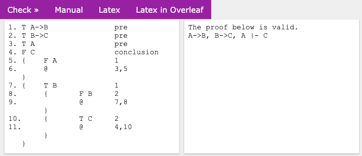
(a) ANITA: $A\rightarrow B,B\rightarrow C,A\vdash C$

[.$T~{}A\rightarrow B$
$T~{}B\rightarrow C$
$T~{}A$
$F~{}C$ [.$F~{}A$ [.$\times$ ] ] [.$T~{}B$ [.$F~{}B$ [.$\times$ ] ] [.$T~{}C$ [.$\times$ ] ] ] ]

(b) Analytic Tableau Proof

(c) Open Branch in ANITA: $A\rightarrow B,B\rightarrow C,A\vdash C$

[.$T~{}A\rightarrow B$
$T~{}B\rightarrow C$
$T~{}A$
$F~{}C$ [.$F~{}A$ [.$\times$ ] ] [.$T~{}B$ ] ]

(d) Analytic Tableau Proof

Figure 17: ANITA: $A\rightarrow B,B\rightarrow C,A\vdash C$

Figure 18 shows a message that the existential-true rule is not applied correctly to signed formula $T~{}Ex~{}H(x)$ in line $1$ to obtain $T~{}H(a)$ in line 4, because the term $a$ is not a new variable (see line $3$).

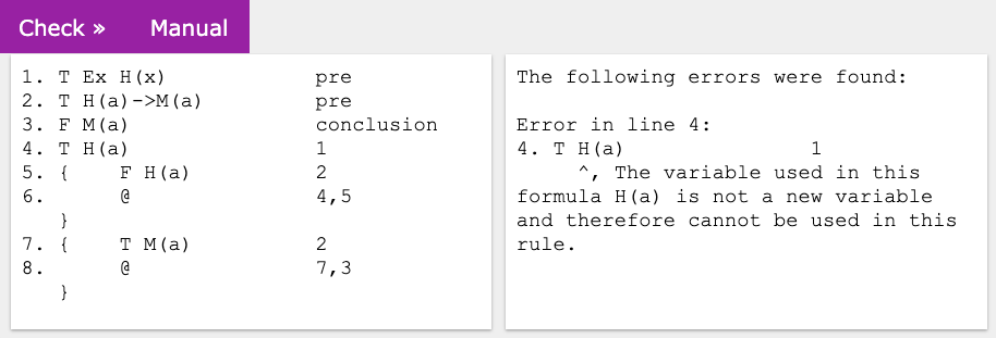
Figure 18: ANITA: An error in a proof

Figure 19(a) presents a proof that $A,A\land B\rightarrow C$ does not entail $C$, and ANITA displays the countermodel of the proof. Figure 19(b) displays the saturated branch in red of the analytic tableau that provides a countermodel that was generated by ANITA. Figure 19(d) displays two saturated branches in red of the analytic tableau that provide countermodels of the proof $A\lor B\not\vdash C$ that were generated by ANITA, see Figure 19(c). Note that in the open branch (lines $1,2$ and $3$) the atomic formula $B$ does not occur, then $v(B)$ can be $T$ or false $F$, and the countermodel is displayed by $v(A)=T,v(C)=F$.

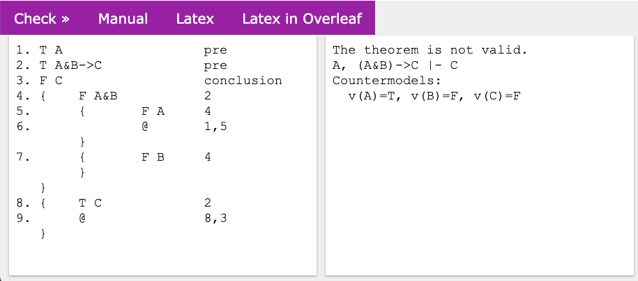
(a) ANITA: $A,A\land B\rightarrow C\not\vdash C$

[.$T~{}A$
$T~{}(A\land B)\rightarrow C$
$F~{}C$ [.$F~{}A\land B$ [.$F~{}A$ [.$\times$ ] ] [.$F~{}B$ ] ] [.$T~{}C$ [.$\times$ ] ] ]

(b) Analytic Tableau Proof

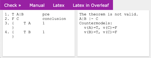
(c) ANITA: $A\lor B\not\vdash C$

[.$T~{}A\lor B$
$F~{}C$ [.$T~{}A$ ] [.$T~{}B$ ] ]

(d) Analytic Tableau Proof

Figure 19: ANITA: Sample of countermodel

5 Related Work

In this article, we focus on Natural Deduction and Analytic Tableau proof assistants. Although, there are proof assistants for other systems, such as SeCaV [6]. We summarize the features of proof assistants, as well as highlight the similarities and differences between these tools and the proposal in this work. We also provide the proof of $A\rightarrow~{}B,B\rightarrow~{}C,A\vdash~{}C$ in each proof assistant.

• The Jape [2] is a desktop proof assistant to write proofs in Fitch-style in Natural Deduction. The proofs are performed by inserting the inference rules through its GUI.

• The ProofWeb [11] is a web interface that intends to be an evolution of JAPE and uses Coq that is state-of-art proof assistant for writing mathematical proofs. The user must write the proofs in a text area or use the GUI to add the inference rules. The ProofWeb can display proofs in Fitch or Gentzen-styles.

• The Panda [7] is also a desktop proof assistant which differs from the previous ones by allowing the writing of proofs in Gentzen-style from its GUI.

• The NaDeA [16] is a web proof assistant for Natural Deduction with a formalization in Isabelle. The user must write the proofs through its user interface which is based on clicking.

• The NADIA [15] is a web proof assistant for Natural Deduction, in Fitch-style. NADIA allows students to write their proofs as closely as possible to the proofs they take on paper, by using an input syntax code similar to [9]. NADIA displays proofs in Fitch or Gentzen-style.

• The Carnap.io [10] is a free and open-source Haskell framework for creating and exploring formal languages, logics, and semantics. A web proof assistant for Analytic Tableaux is available and can be used to construct proofs by using the GUI interface.

• The Tree Proof Generator Tableau is a tableau prover for classical propositional and first-order logic, as well as some modal logics. The prover is written in Javascript and runs entirely in the browser. The user can enter a formula of standard propositional, predicate, or modal logic and the prover will automatically try to find either a countermodel or a tree proof.

ANITA is very similar to NADIA. Both systems receive as input a text with a proof of a theorem and check whether the proof is correct or not. If not, the tools display the errors found. The main difference between the proof assistants is that ANITA accepts proofs in Analytic Tableaux (see Figure 20(a)) and NADIA in Natural Deduction (see Figure 20(b)). The parser of the proofs in ANITA is completely different from the NADIA parser, as each implements a very different set of inference rules.

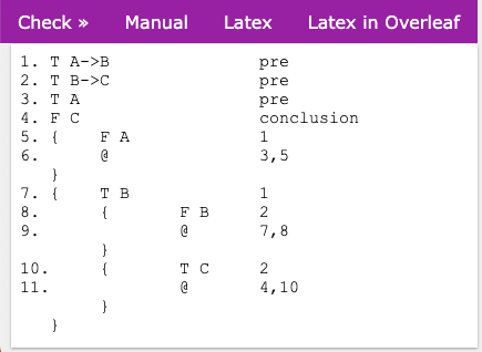
(a) ANITA: $A\rightarrow B,B\rightarrow C,A\vdash C$

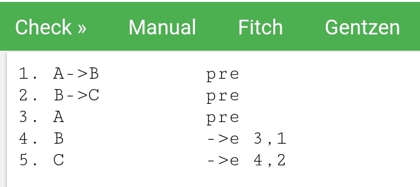
(b) NADIA: $A\rightarrow B,B\rightarrow C,A\vdash C$

Figure 20: ANITA and NADIA Proof Assistants

Figure 21(a) presents a proof in ProofWeb. Note that the student has to learn a new syntax that differs a lot from what the student would write on paper. On the other hand, the proofs in Jape (Figure 21(b)), Panda (Figure 21(c)), NaDeA (Figure 21(d)), and Carnap.io (Figure 22(a)) are carried out by the GUI and the user should click on the menu to add each inference rule. The proof generator, in fact, is a prover instead of proof assistant. So, the user can only interact with the tool to enter the theorem to be get either a countermodel or a tree proof that it is not very useful in order to teach how to use the inference rules.

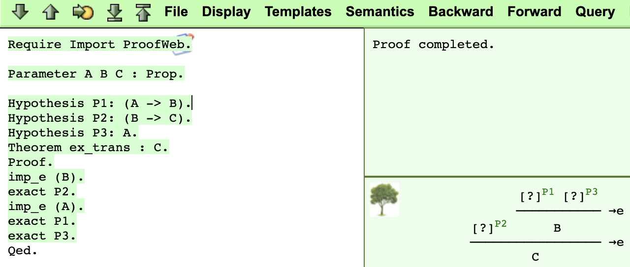
(a) ProofWeb: $A\rightarrow B,B\rightarrow C,A\vdash C$

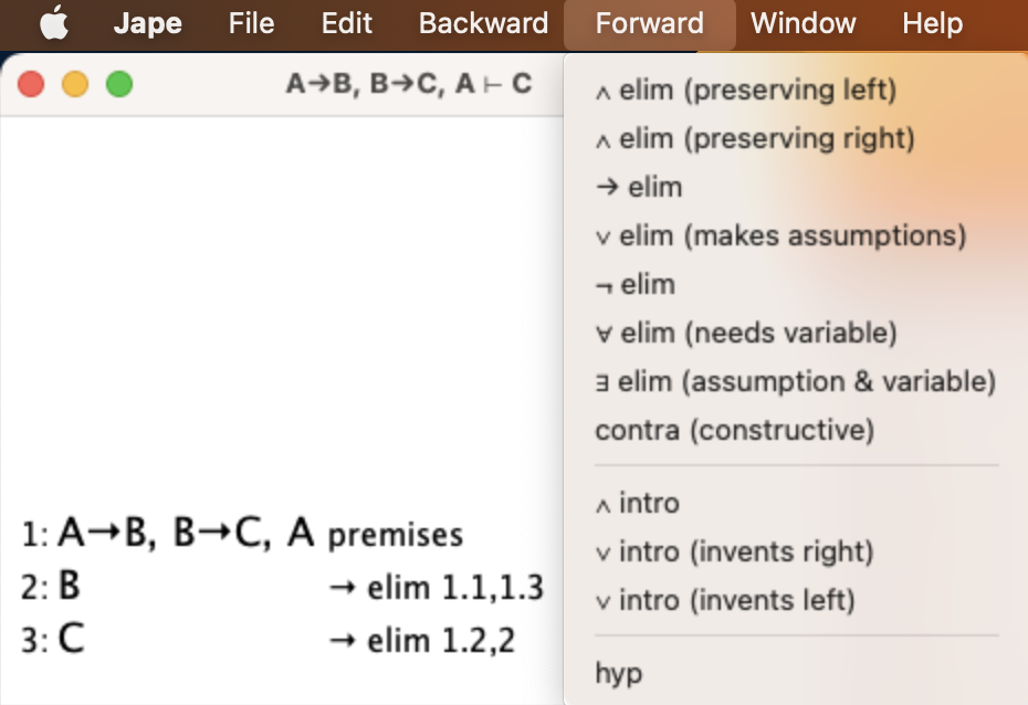
(b) JAPE: $A\rightarrow B,B\rightarrow C,A\vdash C$

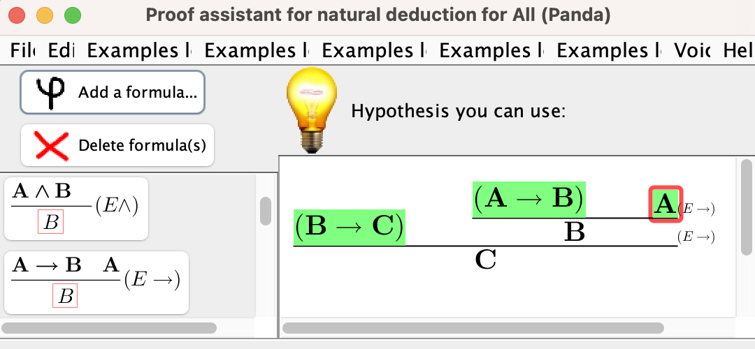
(c) Panda: $A\rightarrow B,B\rightarrow C,A\vdash C$

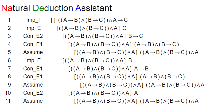
(d) NaDeA: $A\rightarrow B,B\rightarrow C,A\vdash C$

Figure 21: Natural Deduction Tableau Proof Assistants

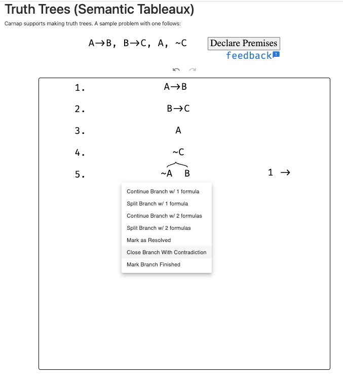
(a) Carnap.io: $A\rightarrow B,B\rightarrow C,A\vdash C$

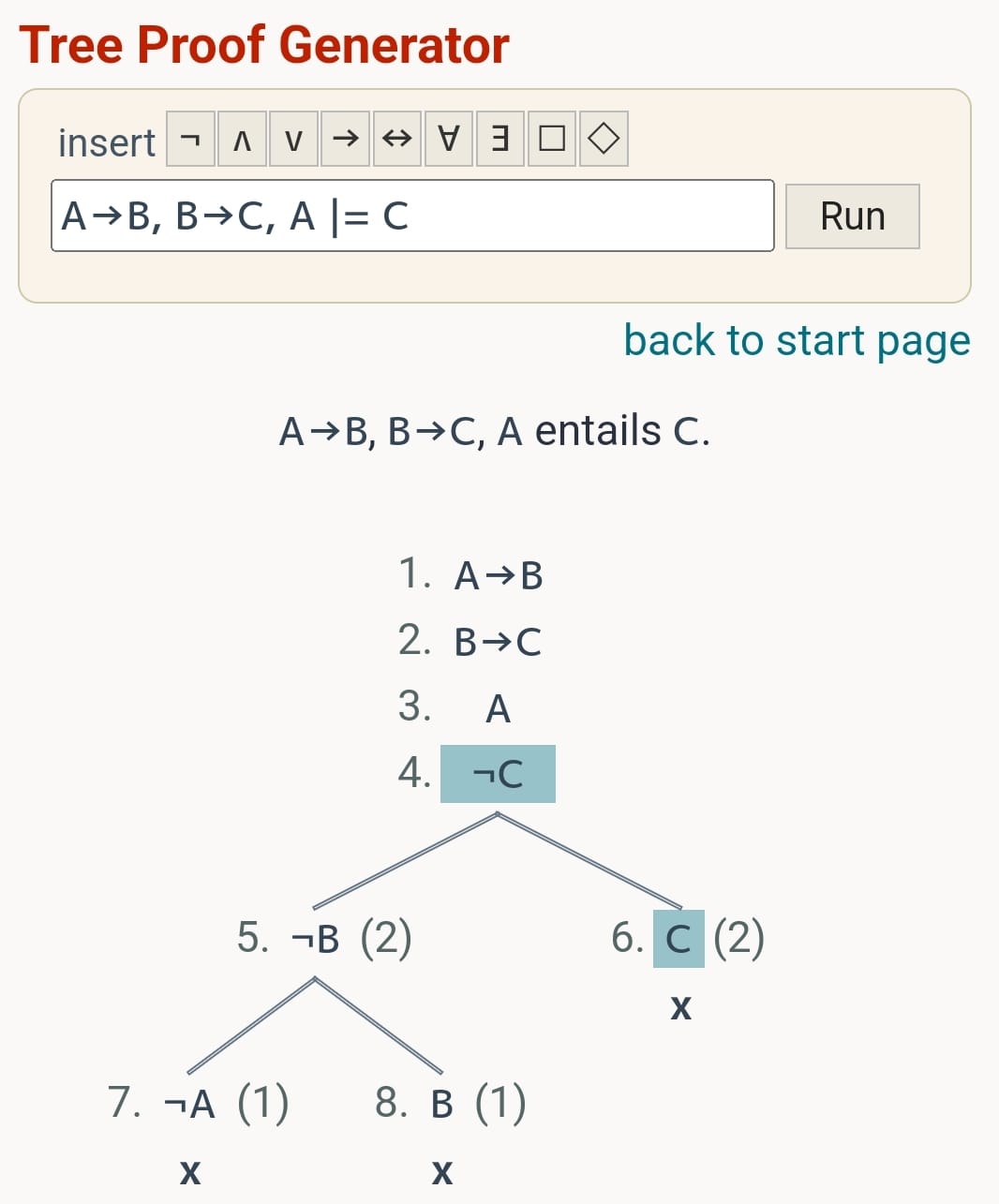
(b) Proof Generator: $A\rightarrow B,B\rightarrow C,A\vdash C$

Figure 22: Analytic Tableau Proof Assistants

Below we summarize the assistant proofs regarding to: the deductive systems (ND for Natural Deduction, AT for Analytic Tableaux); the display of the proof-style (F for Fitch-style, G for Gentzen-style); The input proof-writing (GUI for based on clicking in the GUI interface, PT for plain text).

	ProofWeb	Jape	Panda	NaDeA	NADIA	ANITA	Carnap.io	Proof Gen.
Deductive Systems	ND	ND	ND	ND	ND	AT	AT	AT
Display Proof-Style	F, G	F	G	F	F, G	F	T	T
Input Proof-Writing	GUI, PT	GUI	GUI	GUI	PT	PT	GUI	GUI

6 Evaluation of ANITA

In this section, we present the results of the evaluation of ANITA that were carried out in two classes of Logic in Computer Science in 2022 at the Federal University of Ceará at Quixadá Campus. Each class has 4 hours of class per week and a total of 16 weeks. The classes had a total of 74 students enrolled.

6.1 Student Evaluations of ANITA

In total 36 out of 74 registered students answered the anonymous online form (49%). 100% of the students stated that they used ANITA as a study tool and considered that ANITA helped to exercise the content. 91.7% considered ANITA very easy-to-use. Figure 23(a) shows how often did the students use ANITA and Figure 23(b) shows how they rate ANITA error messages.

(a) How often did you use ANITA?

(b) How do you rate ANITA error messages?

Figure 23: Evaluation

6.2 Evaluation

We used NADIA and ANITA, integrated in the Moodle platform, in the second partial evaluation (AP2), which was applied in the laboratory and had four theorems to be proved in Natural Deduction (ND) and four in analytic Tableaux (AT), each item was worth 1.25. The students wrote down the proofs of each theorem in the Moodle platform and checked automatically, by ANITA and NADIA, whether each proof was correct. For instance, Figure 24(a) displays the answer of a student of Question $1$ of ND in the Moodle platform. Figure 24(b) displays the answer of a student of Question $4$ of AT in the Moodle platform.

(a) Moodle (NADIA) - Answer of Question 1:
$\lnot~{}A\rightarrow(\lnot~{}B\rightarrow~{}C),~{}\lnot~{}B\vdash~{}A\lor~{}C$

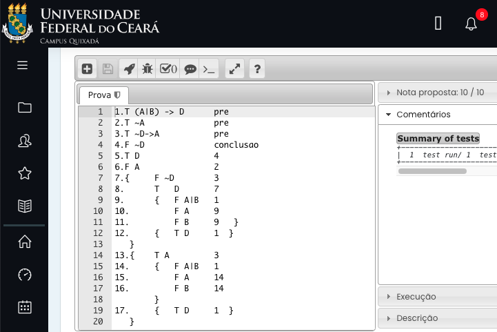
(b) Moodle (ANITA) - Answer of Question 4:
$(A\lor B)\rightarrow D,\lnot A,\lnot D\rightarrow A\not\vdash\lnot D$

Figure 24: AP2 - Samples of questions of NADIA and ANITA in the Moodle Platform

In total 48 out of 74 registered students did the test (65%). The students got a mean (M) of 6.80 with standard deviation (SD) of 3.28. For ND questions, they got 2.76 (MND) and 4.04 (MAT) for AT. 63% (AND) answered the ND questions, of which 87% (RND) got the questions right; 92% (AAT) answered from AT and 88% (RAT) of those answered the questions correctly. Table 1 presents the results by class.

Class	Students	M	SD	MND	SDND	AND	RND	MAT	SDAT	AAT	RAT
A	20	7.31	2.93	2.94	2.08	65%	90%	4.38	1.43	94%	93%
B	28	6.44	3.53	2.64	2.03	62%	85%	3.80	1.82	91%	84%
A+B	48	6.80	3.28	2.76	2,05	63%	87%	4.04	1.66	92%	88%

Table 1: Results by Class

7 Conclusion and Future Work

ANITA has been used for teaching analytic tableaux to computer science students. We have compared ANITA as a tool for teaching logic to other tools. From the evaluation point of view, ANITA has been a success in our courses. 49% of the students answered an anonymous online form, in which: 100% consider that the tool helped to exercise the content;  91% consider the tool easy-to-use (excellent or good);  90% used the tool two or more times a week; and  90% considered the understanding of messages as Excellent or Good. We used ANITA, integrated in the Moodle platform, in the partial evaluation. In total 48 out of 74 registered students did the test (65%). 92% of the students submitted their proofs to 4 theorems and of these 88% got the questions right.

As future work, we consider developing more teaching materials for ANITA and making further evaluations of ANITA as a tool for teaching logic.

Acknowledgements: This work is partially supported by the project 04772314/2020/FUNCAP.

References

- [1]
- [2] Richard Bornat & Bernard Sufrin (1996): Jape’s quiet interface. User Interfaces for Theorem Provers UITP’98.
- [3] M. D’Agostino, D.M. Gabbay, R. Hähnle & J. Posegga (1999): Handbook of Tableau Methods. Springer Netherlands, 10.1007/978-94-017-1754-0.
- [4] Dirk van Dalen (2013): Logic and Structure (5th Ed.). Springer London, London, 10.1007/978-1-4471-4558-5.
- [5] Melvin Fitting (1996): First-Order Logic and Automated Theorem Proving (2nd Ed.). Springer-Verlag, Berlin, Heidelberg, 10.1007/978-1-4612-2360-3.
- [6] Asta Halkjær From, Frederik Krogsdal Jacobsen & Jørgen Villadsen (2022): SeCaV: A Sequent Calculus Verifier in Isabelle/HOL. In Mauricio Ayala-Rincon & Eduardo Bonelli, editors: Proceedings 16th Logical and Semantic Frameworks with Applications, Buenos Aires, Argentina (Online), 23rd - 24th July, 2021, Electronic Proceedings in Theoretical Computer Science 357, Open Publishing Association, pp. 38–55, 10.4204/EPTCS.357.4.
- [7] Olivier Gasquet, François Schwarzentruber & Martin Strecker (2011): Panda: A Proof Assistant in Natural Deduction for All. A Gentzen Style Proof Assistant for Undergraduate Students. In Patrick Blackburn, Hans van Ditmarsch, María Manzano & Fernando Soler-Toscano, editors: Tools for Teaching Logic, Springer Berlin Heidelberg, Berlin, Heidelberg, pp. 85–92, 10.1007/978-3-642-21350-2_11.
- [8] Gerhard Gentzen (1969): The collected papers. North-Holland Publishing Company, 10.2307/2272429.
- [9] Michael Huth & Mark Ryan (2004): Logic in Computer Science: Modelling and Reasoning about Systems (2nd Ed.). Cambridge University Press, 10.1017/CBO9780511810275.
- [10] Graham Leach-Krouse (2018): Carnap: An Open Framework for Formal Reasoning in the Browser. In Pedro Quaresma & Walther Neuper, editors: Proceedings 6th International Workshop on Theorem proving components for Educational software, Gothenburg, Sweden, 6 Aug 2017, Electronic Proceedings in Theoretical Computer Science 267, Open Publishing Association, pp. 70–88, 10.4204/EPTCS.267.5.
- [11] Hendriks Maxim, Cezary Kaliszyk, Femke van Raamsdonk & Freek Wiedijk (2010): Teaching logic using a state-of-art proof assistant. Acta Didactica Napocensia 3. Available at https://files.eric.ed.gov/fulltext/EJ1056118.pdf.
- [12] F.S.C. da Silva, M. Finger & A.C.V. de Melo (2006): Lógica para computação. Cengage Learning. Available at https://books.google.com.br/books?id=w27uOgAACAAJ.
- [13] R.M. Smullyan (1995): First-order Logic. Dover books on advanced mathematics, Dover, 10.1007/978-3-642-86718-7.
- [14] J.N. de Souza (2008): Logica Para Ciencia da Computação. Campus SBC, Elsevier. Available at https://books.google.com.br/books?id=Y8GEsUoRKiEC.
- [15] D. R. Vasconcelos, R. Paula & M. V. Menezes (2022): NADIA - Natural DeductIon proof Assistant. In: Anais do XXX Workshop sobre Educação em Computação, SBC, Porto Alegre, RS, Brasil, pp. 427–438, 10.5753/wei.2022.222875.
- [16] Jørgen Villadsen, Andreas Halkjær From & Anders Schlichtkrull (2018): Natural Deduction and the Isabelle Proof Assistant. In Pedro Quaresma & Walther Neuper, editors: Proceedings 6th International Workshop on Theorem proving components for Educational software, Gothenburg, Sweden, 6 Aug 2017, Electronic Proceedings in Theoretical Computer Science 267, Open Publishing Association, pp. 140–155, 10.4204/EPTCS.267.9.