The Mass Distribution of Quasars in Optical Time-domain Surveys

Abstract

The determination of supermassive black hole (SMBH) masses is the key to understanding the host galaxy build-up and the SMBH mass assembly histories. The SMBH masses of non-local quasars are frequently estimated via the single-epoch virial black-hole mass estimators, which may suffer from significant biases. Here we demonstrate a new approach to infer the mass distribution of SMBHs in quasars by modelling quasar UV/optical variability. Our inferred black hole masses are systematically smaller than the virial ones by $0.3\sim 0.6$ dex; the $\sim 0.3$ dex offsets are roughly consistent with the expected biases of the virial black-hole mass estimators. In the upcoming time-domain astronomy era, our methodology can be used to constrain the cosmic evolution of quasar mass distributions.

1 Introduction

The mass distribution of supermassive black holes (SMBHs) in galaxy centres is vital for our understanding of their mass assembly histories, the active galactic nucleus (AGN) feedback energy budget, and the evolution of host galaxies. For distant AGNs (including quasars, i.e., luminous AGNs with broad emission lines), their SMBH masses ($M_{\rm{BH}}$) are often estimated via the reverberation mapping method (Blandford & McKee, 1982) and its simplified version, the single-epoch virial black-hole mass estimators (for a review, see, e.g., Shen, 2013). The two methods are built upon the assumption that the broad emission-line regions (BLRs), which are photoionized by the central engine and emit broad emission lines, are virialized. The virial mass estimators are calibrated (e.g., Onken et al., 2004) with respect to the famous $M_{\rm{BH}}$–$\sigma$ relation (Ferrarese & Merritt, 2000; Gebhardt et al., 2000) under the assumption that AGNs have similar virial factors. It has been shown that the virial black hole mass ($M_{\rm{BH,vir}}$) has substantial intrinsic uncertainties ($\gtrsim 0.4$ dex) and suffers from systematic biases ($\gtrsim 0.3$ dex; see, e.g., Shen & Kelly, 2010). Ongoing (e.g., Du et al., 2016; Homayouni et al., 2020; Yu et al., 2022) and future reverberation mapping campaigns may considerably improve the accuracy of $M_{\rm{BH,vir}}$ by monitoring a large quasar sample and modelling their BLR structures (e.g., Pancoast et al., 2014; Li et al., 2021).

In the upcoming time-domain era of astronomy, scaling relations between $M_{\rm{BH}}$ and AGN variability properties are often proposed to estimate $M_{\rm{BH}}$ since AGN variability is unambiguous in various wavelengths. Previous studies often focus on the X-ray excess variance and find that the corresponding mass estimation precision is comparable to the reverberation mapping method (e.g., Zhou et al., 2010; Kelly et al., 2013). Some works take an alternative approach by adopting the $M_{\rm{BH}}$-galaxy total stellar mass ($M_{\star}$) scaling relations to model the ensemble X-ray variability and constrain the mass distribution of AGNs in deep X-ray surveys (e.g., Georgakakis, Papadakis, & Paolillo, 2021). In the next decade, the Legacy Survey of Space and Time (LSST) of the Vera C. Rubin Observatory will comprehensively measure AGN variability in the optical bands (e.g., Brandt et al., 2018). While several studies have discussed the possibility to use optical variability to estimate $M_{\rm{BH}}$ (e.g., Kelly & Shen, 2013; Sun et al., 2020; Burke et al., 2021), the validity of such a method has not yet been well demonstrated.

In this study, we aim to constrain the mass distribution of quasars by modelling their optical structure functions measured from the Sloan Digital Sky Survey (SDSS) Stripe 82 (S82; MacLeod et al., 2012) and the Panoramic Survey Telescope and Rapid Response System Survey (Pan-STARRS; Chambers et al., 2016; Flewelling et al., 2020) light curves. The manuscript is formatted as follows. In Section 2, we present the observed quasar variability. In Section 3, we introduce our quasar variability forward modelling procedures. In Section 4, we show the modelling results. Summary and future prospects are made in Section 5.

2 Observations

Following Suberlak, Ivezić, & MacLeod (2021), we use the SDSS S82 quasar light curves and Pan-STARRS observations to explore quasar variations on observed-frame timescales up to $15$ years. The SDSS S82 quasar light curves (each light curve typically contains $40$ data points) are downloaded from https://faculty.washington.edu/ivezic/cmacleod/qso_dr7/Southern.html. Then, we cross-match each SDSS S82 quasar with the Pan-STARRS second data release (https://catalogs.mast.stsci.edu/panstarrs/; each light curve typically has twelve observations) to extend the light-curve duration.

We focus on the $2114$ quasars at redshift $1.4<z<1.8$ because the redshift distribution of our quasar sample peaks at this range. The median redshift for the selected quasars is $1.6$. We cross-match the selected quasars with the quasar property catalogue of Shen et al. (2011) to obtain their bolometric luminosities ($L_{\rm{bol}}$) and $M_{\rm{BH,vir}}$; our conclusions remain unchanged if we use the updated quasar property catalogue of Wu & Shen (2022). The selected quasars are divided into five $\log L_{\rm{bol}}$ bins; each bin has the same number of quasars. Hence, the $\log L_{\rm{bol}}$ bins are defined as follows: [$45.79,45.97$], [$45.97,46.10$], [$46.10,46.25$], [$46.25,46.47$], and [$46.47,46.77$].

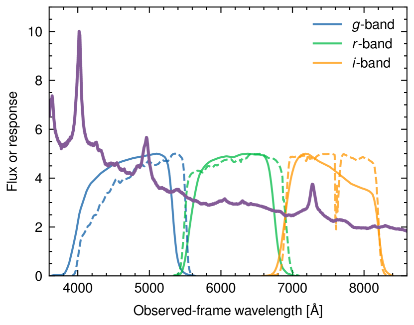
Figure 1: Transmission curves of SDSS (solid curves) and Pan-STARRS (dashed curves) $gri$ bands. The purple curve represents the SDSS composite spectrum at redshift $z=1.6$. Contamination due to strong UV emission lines, e.g., C iv and Ly$\alpha$, are negligible in our studies.

The SDSS S82 data have five bands, i.e., $ugriz$. The Pan-STARRS survey has $grizy$ filters. The SDSS $gri$ and Pan-STARRS $gri$ have similar filter response curves; the SDSS $z$ differ significantly from Pan-STARRS $z$. Hence, we focus on the SDSS and Pan-STARRS $gri$ light curves. For the redshift ranges of our selected quasars, according to the SDSS composite spectrum (Vanden Berk et al., 2001), the $r$-band flux is emission-line free; $g$ and $i$ fluxes have weak inevitable contamination due to Mg ii and C iii] (Figure 1). We assume that such contamination is negligible (see, e.g., MacLeod et al., 2012) in our subsequent analysis.

Following Suberlak, Ivezić, & MacLeod (2021), we use the SDSS S82 standard stars v4.2 of Thanjavur et al. (2021) to find the difference ($\delta m_{\rm{diff}}$) of the SDSS and Pan-STARRS magnitudes at each band as a function of the SDSS $g-r$ colour index,

$$\delta m_{\rm{diff}}=A+B(m_{g}-m_{r})\\ ,$$ (1)

where $m_{g}$ and $m_{r}$ are the apparent magnitudes in SDSS $g$ and $r$ bands, respectively. We use the $g-r$ colour index rather than the $g-i$ one because the $r$ band is emission-line free (Figure 1). For $g$, $r$, and $i$ bands, we find that $A=0.01836$, $0.0009$, and $0.0199$, and $B=0.154$, $0.001$, and $0.008$, respectively. Then, we use the empirical correction of Eq. 1 and quasar $g-r$ colour indexes to convert the observed Pan-STARRS magnitudes into the corresponding SDSS magnitudes and construct merged quasar light curves.

We adopt the SDSS S82 and Pan-STARRS merged light curves to calculate the squared structure functions ($\rm{SF}^{2}$) which measure the statistical variance of quasar magnitude fluctuations ($\Delta m$) at a given band and a fixed rest-frame time separation ($\Delta t$). We consider twenty-two $\Delta t$ which are evenly spaced between rest-frame $1$ day and $2,000$ days in logarithmic space. For each $\Delta t$, the corresponding variability amplitude of $\Delta m$ is calculated via the squared normalized average absolute deviation (squared NAAD),

$$\rm{SF}^{2}(\Delta t)\equiv\sigma_{\rm{NAAD}}^{2}=\frac{\pi}{2}\times\left(\overline{|\Delta m-\overline{\Delta m}|}\right)^{2}\\ ,$$ (2)

where $\overline{\Delta m}$ represents the average value of $\Delta m$; the factor, $\pi/2$, ensures that $\sigma_{\rm{NAAD}}^{2}$ is identical to the variance if the distribution of $\Delta m$ is perfectly Gaussian. We do not subtract $\Delta m$ fluctuations due to magnitude measurement uncertainties. Hence, on very short $\Delta t$ (e.g., $\sim 1$ day), $\sigma_{\rm{NAAD}}^{2}$ traces the measurement uncertainties of $\Delta m$; on timescales of $\geq 10$ days (in rest-frame), $\sigma_{\rm{NAAD}}^{2}$ probes quasar intrinsic variability.

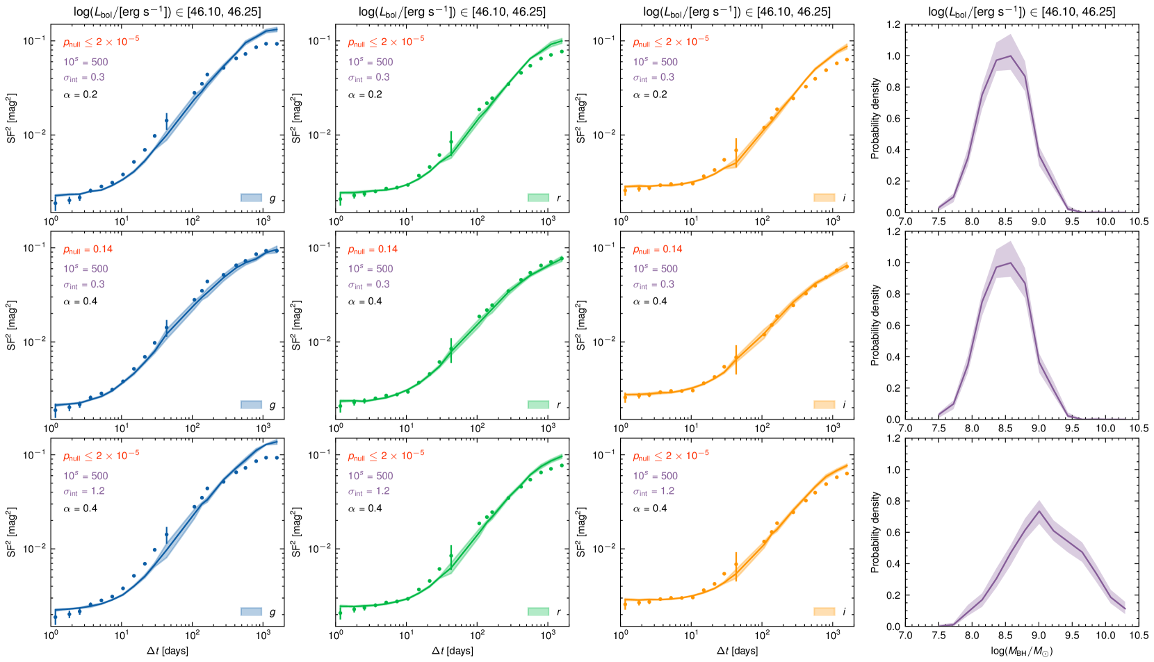
Figure 2: An illustration of the observed (points) squared structure functions versus the model (solid curves) and $1\sigma$ uncertainties (i.e., shaded regions) for models with two different $\alpha$ values or $M_{\mathrm{BH}}$ distributions (shown in the fourth column). The $M_{\mathrm{BH}}$ distributions are controlled by $10^{s}$ and $\sigma_{\mathrm{int}}$. The upper, middle, and bottom rows correspond to models with [$10^{s}=500$, $\sigma_{\rm{int}}=0.3$ dex, $\alpha=0.2$], [$10^{s}=500$, $\sigma_{\rm{int}}=0.3$ dex, $\alpha=0.4$], and [$10^{s}=500$, $\sigma_{\rm{int}}=1.2$ dex, $\alpha=0.4$], respectively. The first, second, and third columns represent the results for $g$, $r$, and $i$ bands, respectively. Panels in the same column have exactly the same observed squared structure functions whose error bars are estimated via $1/N_{\mathrm{p}}$, where $N_{\mathrm{p}}$ is the number of data pairs in each $\Delta t$ bin; error bars are smaller than point sizes in most $\Delta t$ bins. The $p_{\mathrm{null}}$ value is calculated by simultaneously considering the observed squared structure functions of all five luminosity bins and three bands; hence, $p_{\mathrm{null}}$ is the same in each row. The model with [$10^{s}=500$, $\sigma_{\rm{int}}=0.3$ dex, $\alpha=0.4$] fits the observations better than other two models with either different $\alpha$ or $\sigma_{\rm{int}}$. Note that the results in this figure are for the luminosity bin $46.10\leq\log(L_{\rm{bol}}/[\rm{erg\ s^{-1}}])<46.25$; the results for other four luminosity bins are presented in Appendix A.

The observed squared structure functions are shown in Figure 2. As shown in previous SDSS S82 studies (e.g., MacLeod et al., 2012; Suberlak, Ivezić, & MacLeod, 2021), the squared structure functions increase with $\Delta t$ and anti-correlate with wavelengths and quasar luminosities, which agree well with the Corona Heated Accretion disc Reprocessing (CHAR) model predictions (Sun et al., 2020). It has been shown that the CHAR model can reproduce the ensemble structure functions of SDSS S82 light curves (Sun et al., 2020).

3 Modelling the observed structure functions

Table 1: The normalization ($10^{s}$) and intrinsic scatter ($\sigma_{\rm{int}}$) of the $M_{\rm{BH}}$-$M_{\star}$ relation

Case	$10^{s}$	$\sigma_{\rm{int}}$
1	500	0.3
2	500	0.6
3	500	1.2
4	1000	0.3
5	1000	0.6
6	1000	1.2
7	2000	0.3
8	2000	0.6
9	2000	1.2
10	4000	0.3
11	4000	0.6
12	4000	1.2
13	8000	0.3
14	8000	0.6
15	8000	1.2

We use the CHAR model (for the implemented physics, please refer to Sun et al., 2020) to generate mock light curves; then, we compare the squared structure functions of the mock data with the observed ones. SMBHs are assumed to be Schwarzschild black holes, and the inner and outer boundaries of the accretion discs are $3\ R_{\rm{S}}$ and $3000\ R_{\rm{S}}$ (where $R_{\rm{S}}$ is the Schwarzschild radius), respectively. To use the CHAR model, we have to assign four parameters, namely, $L_{\rm{bol}}$, $M_{\rm{BH}}$, the dimensionless viscosity parameter $\alpha$, and the variability amplitude ($\delta_{\rm{mc}}$) of the magnetic fluctuations in the CHAR model. We consider two cases for $\alpha$, i.e., $\alpha=0.2$ and $\alpha=0.4$ (e.g., King, Pringle, & Livio, 2007). We also assume that $\delta_{\rm{mc}}$ is independent of $M_{\rm{BH}}$ or $L_{\rm{bol}}$, which are the remaining two parameters.

Different from our previous study (Sun et al., 2020, which only uses SDSS S82 light curves and probes rest-frame timescales of $\Delta t\lesssim 500$ days), we now do not fix the model $M_{\rm{BH}}$ to $M_{\rm{BH,vir}}$ since the latter suffers from various biases and has substantial uncertainties (for a review, see, e.g., Shen, 2013). Instead, we take a forward-modelling approach and consider the correlation between $M_{\rm{BH}}$ and the total stellar mass ($M_{\star}$) of their host galaxies (e.g., Sun et al., 2015; Li et al., 2021, and references therein), i.e.,

$$\log(M_{\rm{BH}}/M_{\odot})=\log(M_{\star}/M_{\odot})-s\\ ,$$ (3)

with the intrinsic scatter follows a log-normal distribution, whose standard deviation is $\sigma_{\rm{int}}$. We assume that the probability density function of $M_{\star}$ is a summation of two Schechter functions, and we adopt the continuity model parameters (at redshift $z=1.6$) obtained by Leja et al. (2020, see their appendix B). For the value of $s$ (i.e., the normalization of the scaling relation), we consider five cases, i.e., $10^{s}=500$, $1000$, $2000$, $4000$, and $8000$, respectively. For $\sigma_{\rm{int}}$, we explore three values, i.e., $\sigma_{\rm{int}}=0.3$ dex, $0.6$ dex, and $1.2$ dex, respectively. That is, we consider $5\times 3=15$ cases (for a summary, see Table 1). It should be noted that this approach is equivalent to assuming a specific intrinsic distribution of $\log M_{\rm{BH}}$, which is a convolution of the summation of two Schechter functions and a normal distribution (whose mean and standard deviation are $s$ and $\sigma_{\rm{int}}$, respectively). Due to various selection effects, the $\log M_{\rm{BH}}$ distribution of the observed quasars are different from the intrinsic one. Below, we will simulate the detectable mock quasars by applying selection cuts to the intrinsic $\log M_{\rm{BH}}$ distribution.

Our mock light-curve simulation process is similar to that of Georgakakis, Papadakis, & Paolillo (2021). First, we randomly sample mock galaxies (with $M_{\star}$) according to the galaxy stellar mass function of Leja et al. (2020). Second, for each mock galaxy, we assign an SMBH with $M_{\rm{BH}}$ according to Eq. 3. Third, we assume the Eddington ratio distribution of AGNs follows the Schechter function, i.e.,

$$\frac{dt}{d\log\lambda_{\rm{Edd}}}\propto\left(\frac{\lambda_{\rm{Edd}}}{\lambda_{\rm{Edd,cut}}}\right)^{-\gamma}\exp(-\lambda_{\rm{Edd}}/\lambda_{\rm{Edd,cut}})\\ ,$$ (4)

where $\lambda_{\rm{Edd}}$ represents the Eddington ratio; the slope $\gamma$ and $\lambda_{\rm{Edd,cut}}$ are fixed to be $0.2$ and $0.4$ (Jones et al., 2016), respectively. The lower limit of $\log\lambda_{\rm{Edd}}$ is fixed to be $-4$ (i.e., much smaller than the observed $\log\lambda_{\rm{Edd}}$ for quasars) for Case 1; the lower limits of $\lambda_{\rm{Edd}}$ for other cases are adjusted to ensure that their corresponding mean values of $\log L_{\rm{bol}}$ are identical to that of Case 1. Note that our models can reproduce the observed quasar luminosity function. Fourth, we calculate the corresponding bolometric luminosity ($L_{\rm{bol}}$) and convert it into the $3000\ \rm{\AA}$ continuum luminosity ($L_{3000}$, i.e., $\lambda L_{\lambda}$ at $\lambda=3000\ \rm{\AA}$) by adopting a constant bolometric correction of $5$ (whose intrinsic scatter follows a log-normal distribution with the standard deviation of $0.3$), and obtain the corresponding $i$-band apparent magnitude ($m_{i}$) and the FWHM of Mg ii (see Eq. 8 in Shen et al., 2011). Fifth, we select mock quasars with $m_{i}$ brighter than $20.3$ mag and the FWHM of Mg ii larger than $10^{3}\ \rm{km\ s^{-1}}$ (hereafter the “detectable” mock quasars); the $m_{i}$ limit of $20.3$ mag corresponds to the 95-th percentile of the $m_{i}$ distribution of the $2114$ quasars in Section 2. Sixth, for each luminosity bin introduced in Section 2, we randomly select the same number of mock quasars whose $L_{\mathrm{bol}}$ (i.e., $5L_{3000}$) fall into the luminosity bin. Seventh, for each selected mock quasar, we use its $L_{\rm{bol}}$ and $M_{\rm{BH}}$ and the CHAR model to calculate their multi-wavelength light curves. The mock light curves share the same sampling pattern as real observations. In this procedure, $\delta_{\rm{mc}}$ (i.e., the magnetic fluctuation amplitude) is unknown and should be determined according to observations. To save the computation time, we calculate the mock light curves for a given $\delta_{\rm{mc}}$ (denoted as $\delta_{\rm{mc,0}}$), which is independent of $L_{\rm{bol}}$, $M_{\rm{BH}}$, and $\alpha$. The model ensemble squared structure functions for other choices of $\delta_{\rm{mc}}$ can be obtained by multiplying the factor $c=(\delta_{\rm{mc}}/\delta_{\rm{mc,0}})^{2}$ with the model squared ensemble structure functions for $\delta_{\rm{mc,0}}$. Finally, we calculate the model ensemble squared structure functions ($SF^{2}_{\rm{mock}}$) with the same methodology aforementioned. We repeat the calculation $64$ times to estimate the statistical dispersion of a squared structure function.

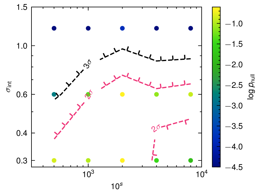
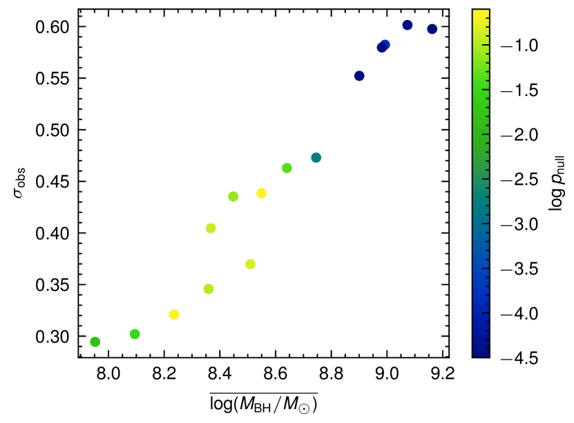
Figure 3: Left: the “allowed” normalization and intrinsic scatter of the $M_{\rm{BH}}-M_{*}$ relation for $\alpha=0.4$. The colours of data points correspond to the null hypothesis probability (i.e., if the model is true, the probability to generate the observed or even larger discrepancy between the data and the model prediction). The black and pink dashed curves indicate the parameter space with $\log p_{\rm{null}}>-1.3$ (i.e., $2\sigma$) and $\log p_{\rm{null}}>-2.6$ (i.e., $3\sigma$). No model has $\log p_{\rm{null}}>-0.49$ (i.e., $1\sigma$). Right: The average and NAAD of the $M_{\mathrm{BH}}$ distributions for mock quasars that are “detectable” (i.e., brighter than $20.34$ mag in the $i$-band and have broad emission lines). Due to the selection effects, there is a clear correlation between the mean and NAAD of the mass distributions of the “detectable” mock quasars.

We use the following statistic for each luminosity bin and each band to fit the model against the data and determine $\delta_{\rm{mc}}$, i.e.,

$$\chi^{2}_{\rm{p},L,\lambda}={} \sum\frac{(\log SF_{\rm{obs}}^{2}-\log(c\times SF_{\rm{mock}}^{2}+SF_{\rm{err}}^{2}))^{2}}{\sigma_{\rm{tot}}^{2}}$$ (5)

$$+\sum\ln(2\pi\sigma_{\rm{tot}}^{2})\ ,$$

where $SF^{2}_{\rm{err}}$ represents the squared ensemble structure function due to magnitude measurement errors. Note that $SF^{2}_{\rm{err}}$ depends upon $L$ and $\lambda$ (see the observed squared structure functions on short timescales in Figure 2). The variance $\sigma_{\rm{tot}}^{2}=(c^{2}\sigma_{\rm{SF}}^{2}+\sigma_{\rm{err}}^{2})/(\ln(10)\times(c\times SF_{\rm{mock}}^{2}+SF_{\rm{err}}^{2}))^{2}$, where $\sigma^{2}_{\rm{SF}}$ and $\sigma^{2}_{\rm{err}}$ represent the variance of $SF_{\rm{mock}}^{2}$ and $SF_{\rm{err}}^{2}$, respectively. We then use Scipy’s optimization function to find the best-fitting parameters that minimizes

$$\chi^{2}_{\rm{p}}=\sum{\chi^{2}_{\rm{p},L,\lambda}}\\ .$$ (6)

There are sixteen free parameters: the first one is $c$, and the remaining fifteen ones are for $SF^{2}_{\rm{err}}$ (five luminosity bins and three bands) which are well determined by $SF^{2}_{\rm{obs}}$ on timescales of $\leq 4$ days.

To measure the goodness of fit, we compute the two-sample Anderson-Darling test statistic ($A_{\rm{obs}}$) between the observed and best-fitting mock squared structure functions for each luminosity bin and each band. We only use data points with $\Delta t>10$ days since the structure functions are dominated by measurement errors on shorter timescales. Indeed, the squared ensemble structure functions on $\Delta t\lesssim 10$ days are larger than those on $\Delta t=1$ day by a factor of $1.2\sim 2.0$ (with a median value of $1.4$), i.e., the intrinsic quasar squared ensemble structure functions are $20\%\sim 100\%$ of those due to measurement errors. Then, we adopt the “random subset selection” (RSS) method (which is widely used in the interpolated cross-correlation analysis) to assess the distribution of the statistic of the Anderson-Darling test. That is, we randomly select (with replacement) $N$ data points from an observed structure function with $N$ data points; only data points with unique $\Delta t$ are used to construct a “fake” structure function; if the data point of the “fake” structure function is larger than ten, we apply the two-sample Anderson-Darling test to the observed and “fake” structure functions and store the corresponding statistic ($A_{\rm{fake}}$). We repeat these procedures $10,000$ times. For each luminosity bin at each band, we can obtain the NAAD of the Anderson-Darling test statistic ($\sigma_{A}$). The final statistic ($A_{\rm{obs,tot}}$) between the best-fitting and observed structure functions for all luminosity bins and bands is the weighted average of $A_{\rm{obs}}$ in each luminosity bin and band and the weighting factor is $1/\sigma_{A}^{2}$. We can also obtain the corresponding fake total statistic ($A_{\rm{fake,tot}}$), which is the weighted average of $A_{\rm{fake}}$, for the $20,000$ RSS simulations. If the best-fitting and observed structure functions are the same (the null hypothesis), we expect that the probability ($p_{\rm{null}}$) for having $A_{\rm{fake,tot}}\geq A_{\rm{obs,tot}}$ in the $10,000$ RSS simulations is not small. Given that we have $20,000$ RSS simulations, if none of $A_{\rm{fake,tot}}$ is larger than $A_{\rm{obs,tot}}$, we can conclude that $p_{\rm{null}}\lesssim 0.5/20000=2\times 10^{-5}$. We reject models with $p_{\rm{null}}<0.05$ (i.e., $\log p_{\rm{null}}<-1.3$).

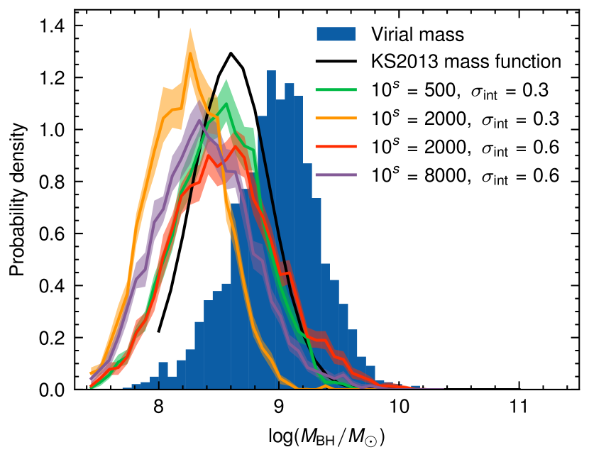
Figure 4: The distributions of $\log M_{\rm{BH}}$ for the four cases with the highest $p_{\rm{null}}$ values (the green, yellow, red, and purple curves). The blue-shaded regions represent the distribution of the virial black-hole mass ($\log M_{\rm{BH,vir}}$). The black curve shows the black-hole mass function of KS2013. Our $\log M_{\rm{BH}}$ is, on average, smaller than $\log M_{\rm{BH,vir}}$ by $0.3\sim 0.6$ dex. The mean $\log M_{\mathrm{BH}}$ values of the models with [$10^{s}=500$, $\sigma_{\rm{int}}=0.3$ dex] and [$10^{s}=2000$, $\sigma_{\rm{int}}=0.6$ dex] are slightly smaller than KS2013 by $0.12$ dex and $0.06$ dex, respectively.

4 Results

We compare models with the same $s$ and $\sigma_{\rm{int}}$ but different $\alpha$. As an illustration, we fix $10^{s}=500$ and $\sigma_{\rm{int}}=0.3$ dex and present the model squared structure functions with $\alpha=0.2$ ($\alpha=0.4$) in the upper (middle) rows of Figure 2. The model with $\alpha=0.2$ fits the observed squared structure functions poorly and its $p_{\rm{null}}$ is much smaller than the alternative model with $\alpha=0.4$. In fact, for all the 15 models with $\alpha=0.2$, their corresponding $p_{\rm{null}}$ are much smaller than $0.04\%$. Hence, the model squared structure functions with $\alpha=0.2$ are statistically rejected for these luminous quasars (with $L_{\rm{bol}}\gtrsim 10^{45.9}\ \rm{erg\ s^{-1}}$). In the subsequent analysis, we focus on models with $\alpha=0.4$.

We can now compare model squared structure functions of various $\alpha=0.4$ models with observed ones. The model and observed squared structure functions for [$10^{s}=500$, $\sigma_{\rm{int}}=0.3$ dex] and [$10^{s}=500$, $\sigma_{\rm{int}}=1.2$ dex] (both with $\alpha=0.4$) are presented in Figure 2. Unlike the latter model (with $p_{\rm{null}}\lesssim 2\times 10^{-5}$), the former one (with $p_{\rm{null}}=0.14$) is not statistically rejected by the observations, demonstrating the possibility to constrain $M_{\rm{BH}}$ distributions from quasar variability.

We can calculate the goodness of fit between the observed and model squared structure functions for different choices of $s$ and $\sigma_{\rm{int}}$ which are the normalization and intrinsic scatter of the $M_{\rm{BH}}$-$M_{\star}$ relation, respectively. The results (corresponding to $\alpha=0.4$) are presented in the left panel of Figure 3. Cases with $\sigma_{\rm{int}}\geq 1.2$ dex have $\log p_{\rm{null}}<-2.7$ (i.e., $p_{\rm{null}}<0.2\%$, which is smaller than the probability to be outside the $3\sigma$ regions of a Gaussian distribution) and are firmly rejected. Case 1 (i.e., $10^{s}=500$ and $\sigma_{\rm{int}}=0.3$ dex) can explain the observed structure functions, which is consistent with recent results of the non-evolution of the $M_{\rm{BH}}$–$M_{\star}$ relation (e.g., Sun et al., 2015; Li et al., 2021). In the right panel of Figure 3, we plot the mean ($\overline{\log(M_{\rm{BH}}/M_{\odot})}$) and NAAD ($\sigma_{\rm{obs}}$) of the black-hole mass distributions of “detectable” mock quasars for all cases. Due to the selection effects (i.e., one can only detect luminous quasars), there is a clear correlation between $\overline{\log(M_{\rm{BH}}/M_{\odot})}$ and $\sigma_{\rm{obs}}$. The model squared structure functions of cases with $\overline{\log(M_{\rm{BH}}/M_{\odot})}=8.2\sim 8.6$ and $\sigma_{\rm{obs}}=0.3\sim 0.45$ dex are similar to the observed ones and have large $p_{\rm{null}}$ (the right panel of Figure 3).

We show the distributions of $\log M_{\rm{BH}}$ for the four cases with highest $p_{\rm{null}}$ (see solid curves with shaded regions in Figure 4). Comparing with $\log M_{\rm{BH,vir}}$, our $\log M_{\rm{BH}}$ for the four cases are systematically smaller by $0.3\sim 0.6$ dex. This systematic offset likely resembles the systematic biases of virial black-hole mass as mentioned by (Shen & Kelly, 2010, see their figure 2). Kelly & Shen (2013, hereafter KS2013) modelled these biases and inferred the bias-corrected $\log M_{\rm{BH}}$ distribution from $\log M_{\rm{BH,vir}}$ for SDSS detected quasars. The $\log M_{\rm{BH}}$ distributions for the two cases with [$10^{s}=500$, $\sigma_{\rm{int}}=0.3$ dex] and [$10^{s}=2000$, $\sigma_{\rm{int}}=0.36$ dex] are on average smaller than KS2013 by only $0.12$ dex or $0.06$ dex, respectively. For the other two cases, the $\log M_{\rm{BH}}$ distributions are on average smaller than that of KS2013 by no more than $0.4$ dex. Hence, in our opinion, the inferred mass distribution is acceptable.

5 Summary and Future Prospects

In this work, we have demonstrated the possibility to infer the $M_{\rm{BH}}$ distribution of quasars by modelling their UV/optical multi-wavelength ensemble structure functions. Some of our $M_{\rm{BH}}$ distributions is roughly consistent with the previous study of Kelly & Shen (2013) that fully accounts for the statistical biases of $M_{\rm{vir,BH}}$. Comparing with existing quasar $M_{\mathrm{BH}}$ measurement methods, our approach does not rely on the knowledge of the unknown BLR structure. Basing on several assumptions (i.e., all galaxies harbour AGNs, $M_{\mathrm{BH}}$ and $M_{\star}$ are correlated, and the distribution of $M_{\star}$ and AGN Eddington ratios follow the Schechter function; see Section 3), we have also constrained the normalization and intrinsic scatter of the possible correlation between $M_{\rm{BH}}$ and $M_{\star}$ at redshift $z\simeq 1.6$.

Compared with SDSS and Pan-STARRS, LSST can provide deeper (by $3\sim 5$ mag) and higher cadence time-domain surveys (e.g., Brandt et al., 2018). Hence, its data can extend our analysis to lower black-hole mass ranges. We can also explore complex models involving different Eddington ratio distributions, the black-hole mass distributions, and SMBH spins. The results can also be used to calibrate the virial black hole at various redshifts.

Data Availability

The SDSS S82 light curves can be downloaded from https://faculty.washington.edu/ivezic/cmacleod/qso_dr7/Southern.html. The Pan-STARRS second data release site is https://catalogs.mast.stsci.edu/panstarrs/. The CHAR model light curves are available upon reasonable request.

Appendix A

In this section, we illustrate our modelling results for other luminosity bins (Figures A5, A6, A7, and A8).

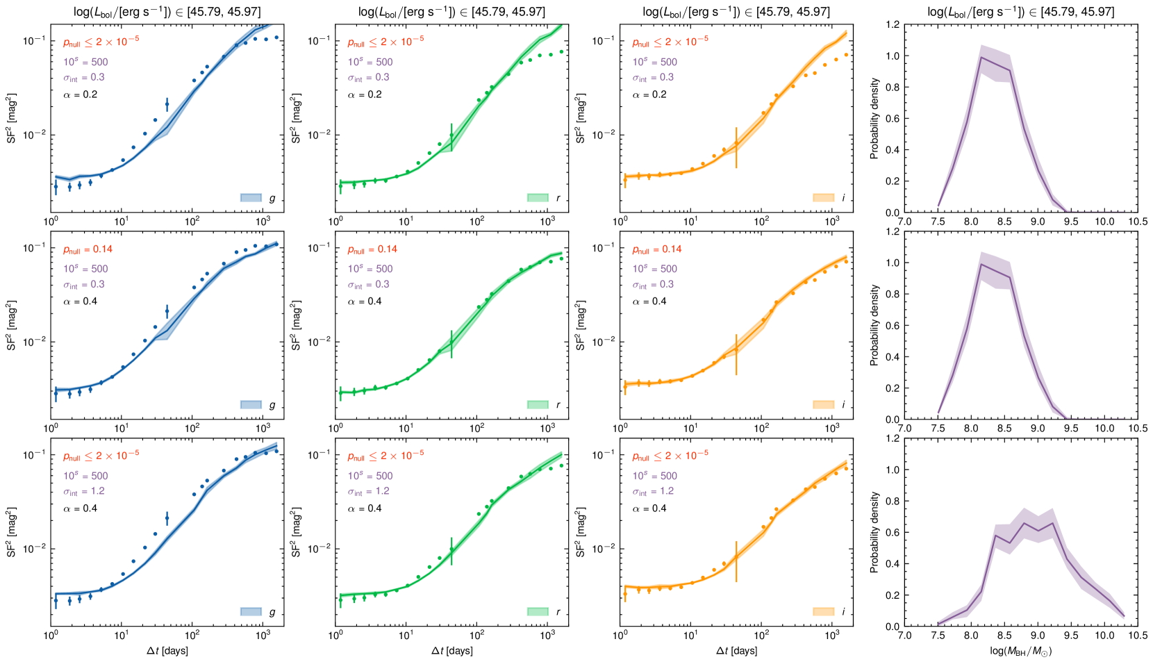
Figure A5: The same as Figure 2, but for the luminosity bin $45.79\leq\log(L_{\rm{bol}}/[\rm{erg\ s^{-1}}])<45.97$.

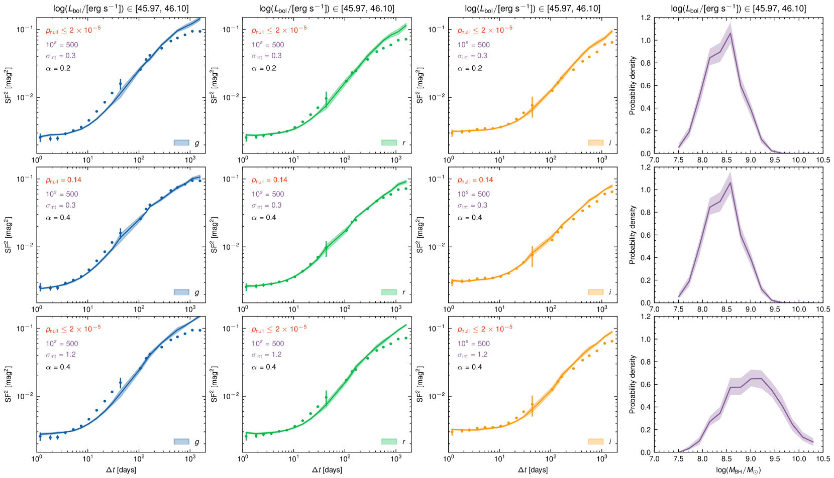
Figure A6: The same as Figure 2, but for the luminosity bin $45.97\leq\log(L_{\rm{bol}}/[\rm{erg\ s^{-1}}])<46.10$.

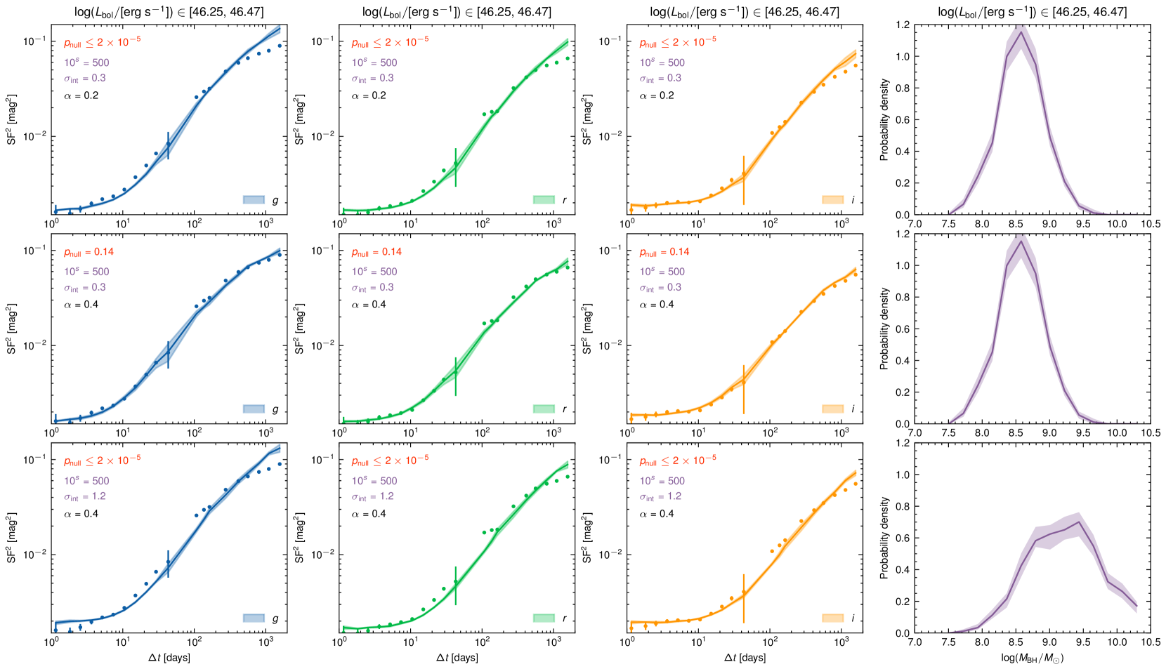
Figure A7: The same as Figure 2, but for the luminosity bin $46.25\leq\log(L_{\rm{bol}}/[\rm{erg\ s^{-1}}])<46.47$.

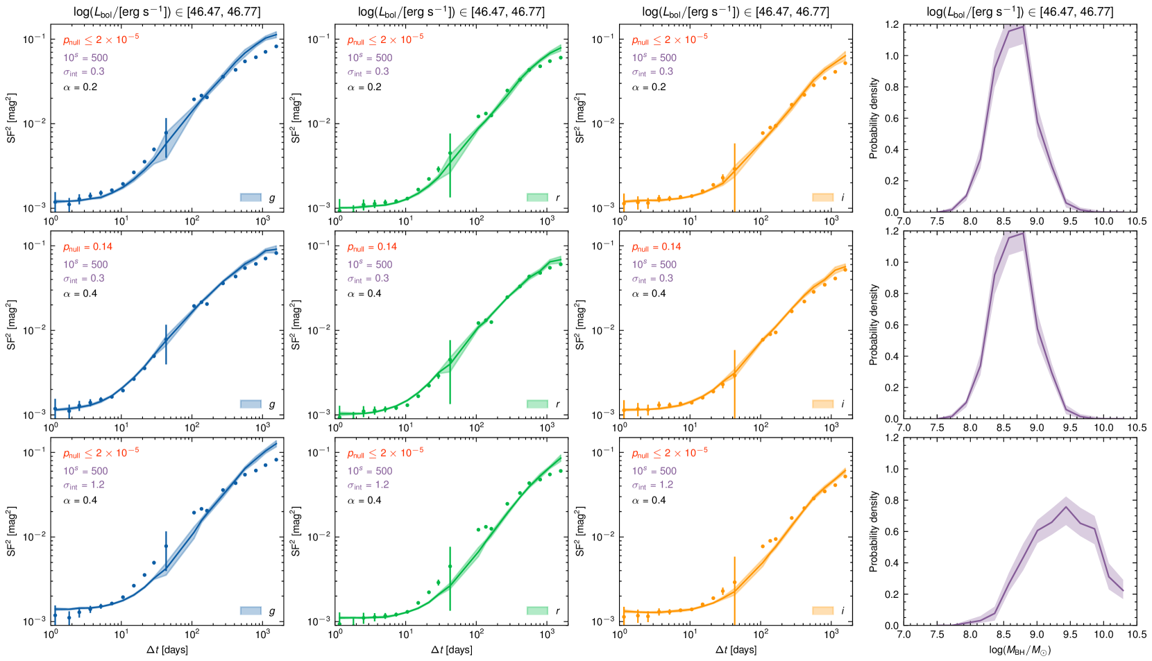
Figure A8: The same as Figure 2, but for the luminosity bin $46.47\leq\log(L_{\rm{bol}}/[\rm{erg\ s^{-1}}])<46.77$.

References

- Aird et al. (2012) Aird J., Coil A. L., Moustakas J., Blanton M. R., Burles S. M., Cool R. J., Eisenstein D. J., et al., 2012, ApJ, 746, 90. doi:10.1088/0004-637X/746/1/90
- Blandford & McKee (1982) Blandford R. D., McKee C. F., 1982, ApJ, 255, 419. doi:10.1086/159843
- Botte et al. (2004) Botte V., Ciroi S., Rafanelli P., Di Mille F., 2004, AJ, 127, 3168. doi:10.1086/420803
- Brandt et al. (2018) Brandt W. N., Ni Q., Yang G., Anderson S. F., Assef R. J., Barth A. J., Bauer F. E., et al., 2018, arXiv, arXiv:1811.06542
- Burke et al. (2021) Burke C. J., Shen Y., Blaes O., Gammie C. F., Horne K., Jiang Y.-F., Liu X., et al., 2021, Sci, 373, 789. doi:10.1126/science.abg9933
- Campana (2017) Campana R., 2017, ascl.soft. ascl:1708.016
- Chambers et al. (2016) Chambers K. C., Magnier E. A., Metcalfe N., Flewelling H. A., Huber M. E., Waters C. Z., Denneau L., et al., 2016, arXiv, arXiv:1612.05560
- Du et al. (2016) Du P., Lu K.-X., Zhang Z.-X., Huang Y.-K., Wang K., Hu C., Qiu J., et al., 2016, ApJ, 825, 126. doi:10.3847/0004-637X/825/2/126
- Ferrarese & Merritt (2000) Ferrarese L., Merritt D., 2000, ApJL, 539, L9. doi:10.1086/312838
- Flewelling et al. (2020) Flewelling H. A., Magnier E. A., Chambers K. C., Heasley J. N., Holmberg C., Huber M. E., Sweeney W., et al., 2020, ApJS, 251, 7. doi:10.3847/1538-4365/abb82d
- Gebhardt et al. (2000) Gebhardt K., Bender R., Bower G., Dressler A., Faber S. M., Filippenko A. V., Green R., et al., 2000, ApJL, 539, L13. doi:10.1086/312840
- Georgakakis, Papadakis, & Paolillo (2021) Georgakakis A., Papadakis I., Paolillo M., 2021, MNRAS, 508, 3463. doi:10.1093/mnras/stab2818
- Homayouni et al. (2020) Homayouni Y., Trump J. R., Grier C. J., Horne K., Shen Y., Brandt W. N., Dawson K. S., et al., 2020, ApJ, 901, 55. doi:10.3847/1538-4357/ababa9
- Hunter (2007) Hunter J. D., 2007, CSE, 9, 90. doi:10.1109/MCSE.2007.55
- Jones et al. (2016) Jones M. L., Hickox R. C., Black C. S., Hainline K. N., DiPompeo M. A., Goulding A. D., 2016, ApJ, 826, 12. doi:10.3847/0004-637X/826/1/12
- Kelly & Shen (2013) Kelly B. C., Shen Y., 2013, ApJ, 764, 45. doi:10.1088/0004-637X/764/1/45
- Kelly et al. (2013) Kelly B. C., Treu T., Malkan M., Pancoast A., Woo J.-H., 2013, ApJ, 779, 187. doi:10.1088/0004-637X/779/2/187
- King, Pringle, & Livio (2007) King A. R., Pringle J. E., Livio M., 2007, MNRAS, 376, 1740. doi:10.1111/j.1365-2966.2007.11556.x
- Leja et al. (2020) Leja J., Speagle J. S., Johnson B. D., Conroy C., van Dokkum P., Franx M., 2020, ApJ, 893, 111. doi:10.3847/1538-4357/ab7e27
- Li et al. (2021) Li J., Silverman J. D., Ding X., Strauss M. A., Goulding A., Schramm M., Yesuf H. M., et al., 2021, ApJ, 922, 142. doi:10.3847/1538-4357/ac2301
- Li et al. (2021) Li S.-S., Yang S., Yang Z.-X., Chen Y.-J., Songsheng Y.-Y., Liu H.-Z., Du P., et al., 2021, ApJ, 920, 9. doi:10.3847/1538-4357/ac116e
- MacLeod et al. (2012) MacLeod C. L., Ivezić Ž., Sesar B., de Vries W., Kochanek C. S., Kelly B. C., Becker A. C., et al., 2012, ApJ, 753, 106. doi:10.1088/0004-637X/753/2/106
- McHardy et al. (2007) McHardy I. M., Arévalo P., Uttley P., Papadakis I. E., Summons D. P., Brinkmann W., Page M. J., 2007, MNRAS, 382, 985. doi:10.1111/j.1365-2966.2007.12411.x
- Onken et al. (2004) Onken C. A., Ferrarese L., Merritt D., Peterson B. M., Pogge R. W., Vestergaard M., Wandel A., 2004, ApJ, 615, 645. doi:10.1086/424655
- Pancoast et al. (2014) Pancoast A., Brewer B. J., Treu T., Park D., Barth A. J., Bentz M. C., Woo J.-H., 2014, MNRAS, 445, 3073. doi:10.1093/mnras/stu1419
- Shen (2013) Shen Y., 2013, BASI, 41, 61
- Shen & Kelly (2010) Shen Y., Kelly B. C., 2010, ApJ, 713, 41. doi:10.1088/0004-637X/713/1/41
- Shen et al. (2011) Shen Y., Richards G. T., Strauss M. A., Hall P. B., Schneider D. P., Snedden S., Bizyaev D., et al., 2011, ApJS, 194, 45. doi:10.1088/0067-0049/194/2/45
- Suberlak, Ivezić, & MacLeod (2021) Suberlak K. L., Ivezić Ž., MacLeod C., 2021, ApJ, 907, 96. doi:10.3847/1538-4357/abc698
- Sun et al. (2015) Sun M., Trump J. R., Brandt W. N., Luo B., Alexander D. M., Jahnke K., Rosario D. J., et al., 2015, ApJ, 802, 14. doi:10.1088/0004-637X/802/1/14
- Sun et al. (2020) Sun M., Xue Y., Brandt W. N., Gu W.-M., Trump J. R., Cai Z., He Z., et al., 2020, ApJ, 891, 178. doi:10.3847/1538-4357/ab789e
- Sun et al. (2020) Sun M., Xue Y., Guo H., Wang J., Brandt W. N., Trump J. R., He Z., et al., 2020, ApJ, 902, 7. doi:10.3847/1538-4357/abb1c4
- Thanjavur et al. (2021) Thanjavur K., Ivezić Ž., Allam S. S., Tucker D. L., Smith J. A., Gwyn S., 2021, MNRAS, 505, 5941. doi:10.1093/mnras/stab1452
- Vanden Berk et al. (2001) Vanden Berk D. E., Richards G. T., Bauer A., Strauss M. A., Schneider D. P., Heckman T. M., York D. G., et al., 2001, AJ, 122, 549. doi:10.1086/321167
- van der Walt, Colbert, & Varoquaux (2011) van der Walt S., Colbert S. C., Varoquaux G., 2011, CSE, 13, 22. doi:10.1109/MCSE.2011.37
- Wu & Shen (2022) Wu Q., Shen Y., 2022, ApJS, 263, 42. doi:10.3847/1538-4365/ac9ead
- Yu et al. (2022) Yu Z., Martini P., Penton A., Davis T. M., Kochanek C. S., Lewis G. F., Lidman C., et al., 2022, arXiv, arXiv:2208.05491
- Zhou et al. (2010) Zhou X.-L., Zhang S.-N., Wang D.-X., Zhu L., 2010, ApJ, 710, 16. doi:10.1088/0004-637X/710/1/16