Distributionally Robust Optimization with Probabilistic Group

Abstract

Modern machine learning models may be susceptible to learning spurious correlations that hold on average but not for the atypical group of samples. To address the problem, previous approaches minimize the empirical worst-group risk. Despite the promise, they often assume that each sample belongs to one and only one group, which does not allow expressing the uncertainty in group labeling. In this paper, we propose a novel framework PG-DRO, which explores the idea of probabilistic group membership for distributionally robust optimization. Key to our framework, we consider soft group membership instead of hard group annotations. Our framework accommodates samples with group membership ambiguity, offering stronger flexibility and generality than the prior art. We comprehensively evaluate PG-DRO on both image classification and natural language processing benchmarks, establishing superior performance. Code is available at https://github.com/deeplearning-wisc/PG-DRO.

1 Introduction

A major challenge in training robust models is the presence of spurious correlations—misleading heuristics imbibed within the training dataset that are correlated with most examples but do not hold in general. For example, consider the Waterbirds dataset (Sagawa et al. 2020a), which involves classifying bird images as waterbird or landbird. Here, the target label (bird type) is spuriously correlated with the background, e.g., an image of waterbird has a higher probability to appear on water background. Machine learning models, when trained on such biased datasets using empirical risk minimization (ERM), can achieve high average test accuracy but fail significantly on rare and untypical test examples lacking those heuristics (such as waterbird on land) (Sagawa et al. 2020a; Geirhos et al. 2019; Sohoni et al. 2020). Such disparities in model prediction can lead to serious ramifications in applications where fairness or safety are important, such as facial recognition (Buolamwini and Gebru 2018) and medical imaging (Oakden-Rayner et al. 2020). This calls for the need of ensuring group robustness, i.e., high accuracy on the under-represented groups.

Over the past few years, a line of algorithms (Sagawa et al. 2020a; Zhang et al. 2020; Mohri, Sivek, and Suresh 2019; Goel et al. 2021) have been proposed to improve group robustness. The core idea behind one of the most common algorithms, G-DRO (Sagawa et al. 2020a), involves minimizing the loss for the worst-performing group during training. Despite the promise, existing approaches suffer from a fundamental limitation — they assume each sample belongs to one and only one group, which does not allow expressing the uncertainty in group labeling. For example, in Figure 1, we show samples from the Waterbirds dataset (Sagawa et al. 2020a), where the background consists of features of both land and water, displaying inevitable ambiguity. In such cases of group ambiguity, using hard group labels can result in the loss of information in robust optimization, and disproportionally penalize the model. Taking the landbird in Figure 1 (right) as an example, a hard assignment of the water attribute would incur an undesirably high sample-wise loss for being associated with the land attribute. To date, few efforts have been made to resolve this.

Motivated by this, we propose a novel framework PG-DRO, which performs a distributionally robust optimization using probabilistic groups. Our framework emphasizes the uncertain nature of group membership, while minimizing the worst-group risk. Our key idea is to introduce the “soft” group membership, which relaxes the hard group membership used in previous works. The probabilistic group membership can allow input to be associated with multiple groups, instead of always selecting one group during robust optimization. We formalize the idea as a new robust optimization objective PG-DRO, which scales the loss for each sample based on the probability of a sample belonging to each group. Our formulation thus accommodates samples with group membership ambiguity, offering stronger flexibility and generality than G-DRO (Sagawa et al. 2020a).

As an integral part of our framework, PG-DRO tackles the challenge of estimating the group probability distribution. We aim to provide a solution with (almost) full autonomy without expensive manual group annotation. Our proposed training algorithm PG-DRO can be flexibly used in conjunction with a variety of pseudo labeling approaches generating group probabilities. Our method henceforth alleviates the heavy data requirement in G-DRO, where each sample needs to be annotated with a group label. In particular, we showcase multiple instantiations through pseudo labeling approach using a small amount of group-labeled data (Section 5) or even without any group-annotated data (Appendix A). In all cases, PG-DRO achieves performance comparable to or outperforms G-DRO (Sagawa et al. 2020a), while significantly reducing group annotation.

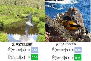
Figure 1: Visual illustration group membership ambiguity. Images are from Waterbirds (Sagawa et al. 2020a) dataset.

Extensive experiments support the superiority of using group probabilities to minimize the worst-group loss. We comprehensively evaluate PG-DRO on both image classification (Section 4.1) and natural language processing (Section 4.2) benchmarks, where PG-DRO establishes state-of-the-art performance. On CelebA (Liu et al. 2015), using only 5% of validation data ($988$ samples), PG-DRO achieves worst-group accuracy of 89.4% and outperforms G-DRO (88.7%) requiring group-annotation on entire train and validation set ($182637$ samples). Lastly, we provide a better understanding of the benefits of our method (Section 6), and validate that PG-DRO effectively learns a more robust decision boundary than G-DRO.

Our key contributions are summarized as follows:

1. We propose PG-DRO, a novel distributionally robust optimization framework for enhancing group robustness. During training, PG-DRO leverages probabilistic group membership, which allows expressing the ambiguity and uncertainty in group labeling. To the best of our knowledge, we are the first to explore the idea of assigning group probabilities as opposed to hard group membership.

2. We perform extensive experimentation on a set of vision and language processing datasets to understand the efficacy of PG-DRO. Specifically, we compare PG-DRO against the five best-performing learning algorithms to date. For both computer vision and NLP tasks, PG-DRO consistently outperforms competing methods and establishes superior performance.

3. We provide extensive ablations to understand the impact of each component in our proposed framework: pseudo group labeling and robust optimization. We observe that irrespective of the pseudo group labeling approach used, PG-DRO consistently outperforms G-DRO in all cases.

2 Preliminaries

In this paper, we consider the problem of learning a classifier when the training data has correlations between true labels and spurious attributes. More generally, spurious attributes refer to statistically informative features that work for the majority of training examples but do not necessarily capture cues related to the labels (Sagawa et al. 2020a; Geirhos et al. 2019; Goel et al. 2021; Tu et al. 2020). Recall the setup in waterbird vs landbird classification problem, where the majority of the training samples has target label (waterbird or landbird) spuriously correlated with the background features (water or land background). Sagawa et al. (Sagawa et al. 2020a) showed that deep neural networks can rely on these spurious features to achieve high accuracy on average, but fail significantly for groups where such correlations do not hold.

Problem Setup. Formally, we consider a training set $\mathcal{D}_{\text{train}}$ consisting of $N$ training samples: $\{\mathbf{x}_{i},y_{i}\}^{N}_{i=1}$. The samples are drawn i.i.d. from a probability distribution: ${\mathcal{P}}_{X,Y}$. Here, $X\in{\mathcal{X}}$ is a random variable defined in the input space, and $Y\in{\mathcal{Y}}=\{1,\ldots,K\}$ represents its label. We further assume that the data is sampled from a set of $E$ environments $\mathcal{E}=\{e_{1},e_{2},\cdots,e_{E}\}$. The training data has spurious correlations, if the input $\mathbf{x}_{i}$ is generated by a combination of invariant features $\mathbf{z}^{\text{inv}}_{i}\in\mathbb{R}^{d_{\text{inv}}}$, which provides essential cues for accurate classification, and environmental features $\mathbf{z}^{e}_{i}\in\mathbb{R}^{d_{e}}$ dependent on environment $e$:

$$\mathbf{x}_{i}=\rho(\mathbf{z}^{\text{inv}}_{i},\mathbf{z}_{i}^{e}).$$

Here $\rho$ represents a function transformation from the feature space $[\mathbf{z}^{\text{inv}}_{i},\mathbf{z}_{i}^{e}]^{\top}$ to the input space ${\mathcal{X}}$. Under the data model, we form groups $g=(y,e)\in\mathcal{Y}\times\mathcal{E}=:\mathcal{G}$ that are jointly determined by the label $y$ and environment $e$.

Based on the data model, each sample $(\mathbf{x},y,g)$ can be denoted as a tuple consisting of input $\mathbf{x}\in{\mathcal{X}}$, label $y\in{\mathcal{Y}}$, and group label $g\in\mathcal{G}$. The standard aim is to train a parameterized model $f_{\theta}:{\mathcal{X}}\rightarrow{\mathcal{Y}}$ that minimizes the expected loss $\mathbb{E}_{(\mathbf{x},y,g)\sim{\mathcal{P}}}[l(f_{\theta}(\mathbf{x}),y)]$ under the training distribution ${\mathcal{P}}$, for some loss function $l:{\mathcal{Y}}\times{\mathcal{Y}}\rightarrow\mathbb{R}_{+}$.

G-DRO.

Sagawa et al. (2020a) proposed group distributionally robust optimization (G-DRO), which minimizes the maximum of the expected loss among the groups:

$$\mathcal{R}_{\text{G-DRO}}(\theta)=\max_{g\in\mathcal{G}}\mathbb{E}_{(\mathbf{x},y)\sim{\mathcal{P}}_{g}}[l(f_{\theta}(\mathbf{x}),y)],$$

where ${\mathcal{P}}_{g}$ indexed by $g\in\mathcal{G}=\{1,2,\cdots,|\mathcal{G}|\}$ denotes group-conditioned data distribution. Given a dataset consisting of $N$ training points $\{\mathbf{x}_{i},y_{i},g_{i}\}^{N}_{i=1}$, G-DRO minimizes the empirical worst-group risk:

$$\hat{f}_{\text{G-DRO}}=\operatorname*{arg\,min}_{\theta\in\Theta}\{\max_{g\in\mathcal{G}}\cfrac{1}{n_{g}}\sum_{i=1}^{N}\mathbb{I}\{g_{i}=g\}l(f_{\theta}(\mathbf{x}_{i}),y_{i})\},$$

where $n_{g}$ represents the number of samples in each group $g\in\mathcal{G}$. In particular, G-DRO assumes that a given sample $\mathbf{x}$ can belong to only one group $g$, which does not allow expressing the uncertainty in group labeling. To see this, in Figure 1, we show examples from Waterbirds dataset (Sagawa et al. 2020a), where the background is associated with both land and water. Using hard group labels in such cases, can encode imprecise information about environmental attributes.

3 Proposed Method

We propose a novel distributional robust optimization framework with probabilistic group (dubbed PG-DRO). Our framework emphasizes the probabilistic nature of group membership, while minimizing the worst-group risk. We proceed to describe the method in detail.

3.1 Robust Optimization Objective

Probabilistic Group.

We first introduce the notion of probabilistic group membership, which relaxes the hard group annotation used in G-DRO. Our key idea is to consider the “soft” probabilities for an input $\mathbf{x}$ to be in environments $\mathcal{E}=\{e_{1},e_{2},\cdots,e_{E}\}$. Formally, we denote $\hat{\mathbb{P}}(e_{i}|\mathbf{x})$ as the estimated probability of an input $\mathbf{x}$ associated with environment $e_{i}$, where:

$$\sum_{i=1}^{E}\hat{\mathbb{P}}(e_{i}|\mathbf{x})=1.$$ (1)

Here we temporarily assume we have some estimation of the probability and we will describe the means of estimation in the following Section 3.2.

Given $\hat{\mathbb{P}}(e_{i}|\mathbf{x})$, the probabilistic group label is defined as a vector $\hat{\mathbb{Q}}(\mathbf{x})\in\mathbb{R}^{|\mathcal{G}|}$ such that:

$$\hat{\mathbb{Q}}(\mathbf{x})_{g}=\begin{cases}\hat{\mathbb{P}}(e_{i}|\mathbf{x})&\text{if $g=(y,e_{i})$,}\\ 0&\text{otherwise}\end{cases}$$ (2)

where $g=\{1,2,\cdots,|\mathcal{G}|\}$ represents group index, and $|\mathcal{G}|=|\mathcal{Y}|\times|\mathcal{E}|$ indicates total number of groups. Note that our definition generalizes the hard group labeling used in G-DRO, where $\hat{\mathbb{Q}}(\mathbf{x})_{g}=1$ for the assigned group and 0 elsewhere.

Probabilistic Group-DRO.

With the definition above, we are ready to introduce our new learning objective called Probabilistic Group-DRO (PG-DRO). Specifically, given $N$ training examples comprising triplets $\{\mathbf{x}_{i},y_{i},\hat{\mathbb{Q}}(\mathbf{x}_{i})\}^{N}_{i=1}$, we define the empirical worst-group risk as :

$$\mathcal{\hat{R}}_{\text{PG-DRO}}(\theta)=\max_{g\in\mathcal{G}}\left\{\cfrac{1}{\widetilde{n}_{g}}\sum_{i=1}^{N}\hat{\mathbb{Q}}(\mathbf{x}_{i})_{g}\cdot l(f_{\theta}(\mathbf{x}_{i}),y_{i})+\cfrac{C}{\sqrt{\widetilde{n}_{g}}}\right\},$$ (3)

where $\hat{\mathbb{Q}}(\mathbf{x}_{i})_{g}$ represents the probability of an input $\mathbf{x}_{i}$ belonging to group $g$, and $C$ is a hyper-parameter modulating model capacity. In effect, the group probability is used as the co-efficient to scale the sample-wise loss. For any group $g\in\mathcal{G}$, we define $\widetilde{n}_{g}=\sum_{i=1}^{N}\hat{\mathbb{Q}}(\mathbf{x}_{i})_{g}$ as the sum of membership of all samples to group $g$. The scaling term $1/\sqrt{\widetilde{n}_{g}}$ constraints the model from overfitting the larger groups and focus on smaller groups. The adjustment parameter $C/\sqrt{\widetilde{n}_{g}}$ helps reduce the generalization gap for each group (Sagawa et al. 2020a). Finally we obtain the optimal model by minimizing the risk in Equation 3:

$$\hat{f}_{\text{PG-DRO}}=\operatorname*{arg\,min}_{\theta\in\Theta}\mathcal{\hat{R}_{\text{PG-DRO}}}(\theta).$$

Note, when $\hat{\mathbb{Q}}(\mathbf{x})$ tends to one-hot encoding for all samples in the training set, indicating that a given input $\mathbf{x}$ is absolutely certain to belong to a particular group, $\mathcal{\hat{R}_{\text{PG-DRO}}}(\theta)$ reduces to $\mathcal{\hat{R}}_{\text{G-DRO}}(\theta)$. PG-DRO henceforth provides a more general and flexible formulation than G-DRO.

3.2 Pseudo Group Labeling

In PG-DRO, towards estimating the probabilistic group labeling $\hat{\mathbb{Q}}(\mathbf{x})$, our aim is to propose a solution with (almost) full autonomy without expensive group annotation manually. Our method alleviates the heavy requirement in G-DRO, where each sample needs to be annotated with group information.

Specifically, given an input $\mathbf{x}$ sampled from a set of environments $\mathcal{E}=\{e_{1},e_{2},...,e_{E}\}$, we would like to first estimate each $\hat{\mathbb{P}}(e_{i}|\mathbf{x})$. For this, we propose training a parameterized classifier $f_{\phi}:{\mathcal{X}}\rightarrow\mathcal{E}$, that can predict the spurious environment attribute $e$. To train the model, we use a small set of group-labeled samples, $\mathcal{D_{\text{L}}}=\{(\mathbf{x}_{1},y_{1},g_{1}),\cdots,(\mathbf{x}_{m},y_{m},g_{m})\}$, such that $m\ll N$. The overall objective function consists of a supervised loss for samples in $\mathcal{D_{\text{L}}}$ :

$$\hat{f}_{\text{env}}=\operatorname*{arg\,min}_{\phi\in\Phi}\{\mathbb{E}_{(\mathbf{x},y,g)\sim{\mathcal{D}_{L}}}[\ell_{\text{CE}}(f_{\phi}(\mathbf{x}),e)]\},$$ (4)

where $g=(y,e)$ and $\ell_{\text{CE}}$ represents standard cross-entropy loss. We use weighted sampling based on the frequency of the samples in $\mathcal{D_{\text{L}}}$. Finally, for every sample $\mathbf{x}\in\mathcal{D}_{\text{train}}$, we use the trained model, $\hat{f}_{\text{env}}$, to predict the probability estimate $\hat{\mathbb{P}}(e|\mathbf{x})$ for each environment $e\in\{e_{1},e_{2},...,e_{E}\}$. We obtain group probabilities, $\hat{\mathbb{Q}}(\mathbf{x})$, as defined in Equation 2 and use it for training PG-DRO.

Remark. Note that our proposed training objective PG-DRO can be flexibly used in conjunction with other pseudo labeling approaches generating group probabilities. Beyond pseudo labeling with supervised loss above, we also showcase the strong feasibility of alternative group labeling approaches. We provide further details in Section 5 and Appendix A.

4 Experiments

In this section, we comprehensively evaluate PG-DRO on both computer vision tasks (Section 4.1) and natural language processing (Section 4.2) containing spurious correlations.

4.1 Evaluation on Image Classification Benchmarks

Method	Dataset with group label	Waterbirds		CelebA
		Avg. Acc	Worst Group Acc	Avg. Acc	Worst Group Acc
ERM (Vapnik 1991)	None	97.3	63.2	95.6	47.2
CVaR DRO (Levy et al. 2020)	val. set	96.0	75.9	82.5	64.4
LfF (Nam et al. 2020)	val. set	91.2	78.0	85.1	77.2
EIIL (Creager, Jacobsen, and Zemel 2021)	val. set	96.9	78.7	91.9	83.3
JTT (Liu et al. 2021)	val. set	93.3	86.7	88.0	81.1
SSA (Nam et al. 2022)	val. set	92.2	89.0	92.8	89.8
PG-DRO (Ours)	val. set	92.5±0.5	91.0±0.6	92.2±0.4	90.0±0.9
G-DRO (Sagawa et al. 2020a)	train & val. set	92.4±0.2	90.7±0.9	92.8±0.3	88.7±1.5

Table 1: Comparison of average and worst-group test accuracies for different methods when evaluated on image classification datasets: Waterbirds (Sagawa et al. 2020a) & CelebA (Liu et al. 2015). We obtain the results of CVaR DRO, LfF, EIIL, JTT and SSA from (Nam et al. 2022). Results (mean and std) of our method are estimated over 3 random runs. Best performing results (in terms of worst-group accuracy) are marked in bold.

Method	Waterbirds			CelebA
	$100\%$	$10\%$	$5\%$	$100\%$	$10\%$	$5\%$
	(Val. set)			(Val. set)
JTT	86.7	86.9	76.0	81.1	81.1	82.2
SSA	89.0	88.9	87.1	89.8	90.0	86.7
PG-DRO	91.0	90.3	89.2	90.0	90.6	89.4

Table 2: Worst-group accuracy on Waterbirds and CelebA under varying fractions of the group-annotated validation set. Our proposed framework, PG-DRO, outperforms state-of-art methods even under reduced group annotation. Results of JTT (Liu et al. 2021) and SSA (Nam et al. 2022) are from (Nam et al. 2022).

Datasets. In this study, we consider two common image classification benchmarks: Waterbirds (Sagawa et al. 2020a) and CelebA (Liu et al. 2015).

(1) CelebA (Liu et al. 2015): Training samples in CelebA have spurious associations between target label and demographic information such as gender. We use the label space $\mathcal{Y}=\{\textsc{blond hair},\textsc{dark hair}\}$ and gender as the spurious feature, $\mathcal{E}=\{\textsc{male},\textsc{female}\}$. The training data consists of $162770$ images with $1387$ in the smallest group, i.e., male with blond hair.

(2) Waterbirds (Sagawa et al. 2020a): Introduced in (Sagawa et al. 2020a), this dataset contains spurious correlation between the background features and target label $y\in$ {waterbird, landbird}. The dataset is constructed by selecting bird photographs from the Caltech-UCSD Birds-200-2011 (CUB) (Wah et al. 2011) dataset and then superimposing on $\mathcal{E}=\{\textsc{water},\textsc{land}\}$ background selected from the Places dataset (Zhou et al. 2017). The dataset consists of $n=4795$ training examples, with the smallest group size 56 (i.e., waterbird on land background).

Training details. For experimentation on image classification datasets, following prior works (Sagawa et al. 2020a) we use ResNet-50 (He et al. 2016) initialized from ImageNet pre-trained model. Models are selected by maximizing the worst-group accuracy on the validation set. We provide detailed description regarding hyper-parameter in Appendix B and C.

Metrics. For all methods, we report two standard metrics: (1) average test accuracy and (2) worst-group test accuracy. In particular, the worst-group test accuracy indicates the model’s generalization performance for groups where the correlation between the label $y$ and environment $e$ does not hold. High worst-group test accuracy indicates a model’s less reliance on the spurious attribute.

PG-DRO outperforms strong baselines.

In Table 1, we show that our approach PG-DRO significantly outperforms all the rivals on vision datasets, measured by the worst-group accuracy. For comparison, we include the best-performed learning algorithms to date: CVaR DRO (Levy et al. 2020), LfF (Nam et al. 2020), EIIL (Creager, Jacobsen, and Zemel 2021), JTT (Liu et al. 2021), and SSA (Nam et al. 2022)—all of which are developed without assuming the availability of group-labeled training data. Similar to ours, these methods utilize a validation set that contains the group labeling information. The comparisons are thus fair given the same amount of information. In addition, we also compare with G-DRO (Sagawa et al. 2020a), which requires the entire training dataset to be labeled with group attribute and hence is significantly more expensive from an annotation perspective.

We highlight two salient observations: (1) On CelebA, PG-DRO outperforms G-DRO by 1.3% in terms of worst-group accuracy. The result signifies the advantage of using probabilistic group labeling compared to hard group labeling. Moreover, our method achieves overall better performance than G-DRO while using significantly less group annotation (validation set only). (2) Among methods that do not use group-labeled training samples, PG-DRO outperforms the current SOTA methods, JTT (Liu et al. 2021) and SSA (Nam et al. 2022), by 4.3% and 2% on Waterbirds dataset respectively. As expected, while ERM consistently achieves the best average accuracy among all methods, its worst-group accuracy suffers the most.

PG-DRO remains competitive under reduced group annotation.

In Table 2, we show that the benefits of using group probabilities persist even when the model is trained with reduced group annotation. Specifically, we perform controlled experiments and compare PG-DRO with two latest SOTA methods, SSA (Nam et al. 2022) and JTT (Liu et al. 2021), in settings where the group labels are available on $100\%$, $10\%$ and $5\%$ of the validation set. We observe that even under reduced group annotation, PG-DRO consistently outperforms both SSA and JTT. In particular, under the challenging setting with only 5% of the validation set, PG-DRO outperforms both SSA and JTT by 2.1% and 13.2% on Waterbirds (Sagawa et al. 2020a) dataset, in terms of worst-group accuracy.

Further, we also include additional qualitative evidence via GradCAM (Selvaraju et al. 2017) visualizations in Appendix E. We observe that for the Waterbirds dataset, PG-DRO consistently focuses on semantic regions representing essential cues for accurately identifying the foreground object such as claw, wing, beak, and fur. In contrast, baseline methods tend to output higher salience for spurious background attribute pixels.

Method	Dataset with group label	MultiNLI		CivilComments-WILDS
		Avg. Acc	Worst Group Acc	Avg. Acc	Worst Group Acc
ERM (Vapnik 1991)	None	82.6	66.4	92.6	58.4
CVaR DRO (Levy et al. 2020)	val. set	82.0	68.0	92.5	60.5
LfF (Nam et al. 2020)	val. set	80.8	70.2	92.5	58.8
EIIL (Creager, Jacobsen, and Zemel 2021)	val. set	79.4	70.9	90.5	67.0
JTT (Liu et al. 2021)	val. set	78.6	72.6	91.1	69.3
SSA (Nam et al. 2022)	val. set	79.9	76.6	88.2	69.9
PG-DRO (Ours)	val. set	81.0±0.4	78.9±0.9	89.2±1.4	73.6±1.8
G-DRO (Sagawa et al. 2020a)	train & val. set	81.4±0.1	77.5±1.2	87.7±0.6	69.1±0.8

Table 3: Comparison of average and worst-group test accuracies for different methods when evaluated on language processing datasets: MultiNLI (Williams, Nangia, and Bowman 2018) & CivilComments-WILDS (Borkan et al. 2019; Koh et al. 2021). We obtain the results of CVaR DRO, LfF, EIIL, JTT and SSA from (Nam et al. 2022). Results (mean and std) of our method are estimated over 3 random runs. Best performing results (in terms of worst-group accuracy) are marked in bold.

4.2 Evaluation on Natural Language Processing Tasks

Datasets.

To validate the effectiveness of PG-DRO, we perform experiments on two natural language processing datasets: MultiNLI and CivilComments-WILDS containing spurious correlations.

(1) MultiNLI (Williams, Nangia, and Bowman 2018): The Multi-Genre Natural Language Inference (MultiNLI) dataset is a crowdsourced collection of sentence pairs with the premise and hypothesis. The label indicates whether the hypothesis is entailed by, contradicts, or is neutral to the premise. Hence, the label space is defined as $\mathcal{Y}=\{\textsc{entailed},\textsc{neutral},\textsc{contradictory}\}$. Previous study (Gururangan et al. 2018) has shown the presence of spurious associations between the target label contradictory and set of negation words, $\mathcal{E}$={nobody, no, never, nothing}.

(2) CivilComments-WILDS (Borkan et al. 2019; Koh et al. 2021): For this dataset, we use a similar setup as defined in  (Nam et al. 2022). Each instance in this dataset corresponds to an online comment generated by users which is labeled as either toxic or not toxic, $\mathcal{Y}=\{\textsc{toxic},\textsc{non-toxic}\}$. The spurious attribute is set as $\mathcal{E}=\{\textsc{identity},\textsc{no identity}\}$, where identity indicates comment associated with any of the demographic identities {male, female, White, Black, LGBTQ, Muslim, Christian, other religion}.

Training details.

For experimentation on language processing tasks, we use a pre-trained BERT model (Devlin et al. 2019). Specifically, we use the Hugging Face PyTorch-Transformers (Wolf et al. 2020) implementation of the BERT bert-base-uncased model. We use the default tokenizer and model settings. The evaluation metrics are the same as Section 4.1. Refer Appendix B and C for detailed description regarding hyper-parameters.

PG-DRO achieves superior performance.

In Table 3, we provide a comprehensive comparison against an array of well-known learning algorithms designed to tackle spurious correlations in training data, including CVaR DRO (Levy et al. 2020), LfF (Nam et al. 2020), EIIL (Creager, Jacobsen, and Zemel 2021), JTT (Liu et al. 2021), and SSA (Nam et al. 2022). For fair evaluation, all competing methods utilize group annotations on the validation set. We also compare against standard baselines such as ERM which does not require group labeling, and G-DRO (Sagawa et al. 2020a) which assumes group labeling information for both train and validation set.

Similar to our observations on vision datasets, PG-DRO upholds the trend of outperforming competing baselines achieving superior performance on both natural language processing tasks. In particular, PG-DRO improves the current best method SSA (Nam et al. 2022) by 3.7% and 2.3% on the CivilComments-WILDS and MultiNLI dataset respectively.

5 Further Ablations

Pseudo Group Labeling Method	Robust Optimization Method	Dataset with group label	Waterbirds		CelebA
			Avg. Acc	Worst Group Acc	Avg. Acc	Worst Group
Supervised	G-DRO	val. set	92.4	88.0	91.6	88.6
	PG-DRO (Ours)	val. set	92.5	91.0	92.2	90.0
Supervised	G-DRO	$5\%$ of val. set	92.5	87.5	92.5	87.5
	PG-DRO (Ours)	$5\%$ of val. set	91.7	89.2	92.0	89.4
Semi-Supervised	G-DRO	val. set	92.2	89.0	92.8	89.8
	PG-DRO (Ours)	val. set	92.4	91.0	92.5	89.8
Semi-Supervised	G-DRO	$5\%$ of val. set	92.6	87.1	92.8	86.7
	PG-DRO (Ours)	$5\%$ of val. set	91.9	89.2	91.7	87.8
Zero-shot	G-DRO	None	91.2	87.6	93.2	87.8
	PG-DRO (Ours)	None	91.5	89.4	92.7	88.8

Table 4: Comparison of average and worst-group test accuracies for different combinations of training objectives used during pseudo group labeling and robust optimization. Best performing results (in terms of worst-group accuracy) are marked in bold.

Given the strong performance of PG-DRO on both computer vision (Section 4.1) and NLP (Section 4.2) tasks, we take a step further to understand the advantages of using probabilistic group membership over hard group annotations. Specifically, in this section, we design controlled experiments to ablate the role of each component in our proposed framework: pseudo group labeling and robust optimization. In particular, for comprehensive evaluation and comparison, we train the spurious attribute classifier ($\hat{f}_{\text{env}}$) using: (1) supervised approach described in Section 3.2, (2) a new zero-shot approach (see details in Appendix A), and (3) semi-supervised learning (Lee et al. 2013; Nam et al. 2022). The semi-supervised objective additionally requires using group unlabelled training samples, in addition to a small number of labeled ones.

PG-DRO outperforms G-DRO under different pseudo group labeling methods.

In Table 4, we provide a comprehensive comparison between PG-DRO and G-DRO for different pseudo group labeling objectives. We observe that for both Waterbirds and CelebA datasets, PG-DRO consistently outperforms G-DRO under different approaches for pseudo group labeling. These results further highlight that the advantages of using probabilistic group membership can be leveraged irrespective of the pseudo group labeling approach used. Moreover, PG-DRO continues its dominance over G-DRO under the most challenging setting, when group annotations are available for only 5% of the validation set. These experiments further underwrite the importance of using probabilistic group membership.

6 Understanding Benefits of PG-DRO

The results in Section 4 and Section 5 validate the improved performance of our proposed framework PG-DRO. In this section, we seek to provide a better understanding for the improved performance.

6.1 Setup

Data distribution.

We construct a synthetic dataset to better understand the advantages of using group-probabilities over hard group annotations. Compared to the complex real datasets studied in Section 4, this synthetic data helps us directly visualize and understand each component of PG-DRO, and its influence on the decision boundary. Specifically, the training dataset ($\mathcal{D}_{\text{train}}$) consists of $n$ training samples: $\{\mathbf{x}_{i},y_{i}\}_{i=1}^{n}$, where the label $y=\{-1,1\}$ is spuriously correlated with the environment attribute $e=\{-1,1\}$. Replicating the real datasets studied in Section 4, we divide the training data into four groups accordingly: two majority groups with $y=e$, each of size $n_{\text{maj}}/2$, and two minority groups with $y=-e$, each of size $n_{\text{min}}/2$. Further, we set $n=n_{\text{maj}}+n_{\text{min}}$ as the total number of training points, and $p=n_{\text{maj}}/n$ as the fraction of majority examples. A higher value of $p$ indicates a stronger correlation between target label $y$ and environment attribute $e$.

An input sample $\mathbf{x}=[z_{\text{inv}},z_{\text{e}}]\in\mathbb{R}^{2}$ comprises of invariant features $z_{\text{inv}}\in\mathbb{R}$ generated from target label $y$, and environmental/spurious features $z_{\text{e}}\in\mathbb{R}$ generated from environment $e$. In particular, we generate:

$$z_{\text{inv}}\sim\mathcal{N}(y,\sigma^{2}_{\text{inv}})$$

$$z_{\text{e}}\sim\mathcal{N}(e,\sigma^{2}_{\text{e}}),$$

The randomness in the invariant and environmental features are controlled through their respective variances. For all experiments in Section 6.2, we fix the total number of training points $n=4000$ and majority fraction $p=0.95$. Further, $\sigma^{2}_{\text{inv}}$ and $\sigma^{2}_{\text{e}}$ are set as 0.5 and 0.05 respectively to encourage the model to use the environmental features over the invariant features.

Model. Both for the purpose of pseudo group labeling and robust optimization, we use a simple four layered neural network with ReLU activation. We provide further details of model training in Appendix.

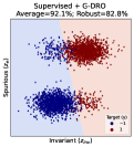
(a)

(b)

Figure 2: Consider data points $\mathbf{x}$ in $\mathbb{R}^{2}$ with two classes $y$. The vertical axis of $\mathbf{x}$ is the environment/spurious feature that highly correlates with $y$, and the horizontal axis is the invariant feature. The data consists of four groups, where the top-left and lower-right are two minority groups. The robust accuracy is test worst-group accuracy. Model trained using PG-DRO (b) is more robust as compared to the G-DRO (a). Color of points encodes ground truth label $y$. Color of background shade indicates model’s prediction $\hat{y}$.

6.2 Insights

PG-DRO leads to a more robust decision boundary than G-DRO. In this study, we train a group predictor on a small group-labeled dataset ($\mathcal{D}_{\text{L}}$) consisting of $100$ samples.

Next, the trained group classifier is used to generate both hard group labels and group probabilities for every sample $\mathbf{x}\in\mathcal{D}_{\text{train}}$ for further training with G-DRO and PG-DRO respectively. In case of G-DRO, $\hat{\mathbb{Q}}(\mathbf{x})$ has all its mass in the predicted group. In Figure 2, we visualize the decision boundary plot of models trained using G-DRO vs. PG-DRO. The vertical axis in the plots indicate the environmental/spurious feature ($z_{\text{e}}$) that highly correlates with $y$, and the horizontal axis is the invariant feature ($z_{\text{inv}}$). We observe that the PG-DRO trained model (Figure 2(b)) learns a more robust decision boundary (more dependent on invariant features) as compared to the model trained using G-DRO (Figure 2(a)). Moreover, the improved worst-group test accuracy of using PG-DRO further validates the advantages of using group probabilities.

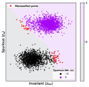
Figure 3: Consider data points $\mathbf{x}\in\mathcal{D}_{\text{train}}$. Color of points encodes the true spurious attribute $e$. (Left) Confidence plot of the trained spurious attribute classifier. We visualize the maximum confidence ($\max_{i}\hat{\mathbb{P}}(e_{i}|x)$) of the spurious predictor. (Right) Decision boundary based on hard labeling. Color of background shade indicates the model’s predicted environment ($\operatorname*{arg\,max}_{i}\hat{\mathbb{P}}(e_{i}|x)$). Mis-classified points are marked in red, which are erroneously penalized with hard labeling. Using probabilistic group better captures uncertainty in spurious attribute prediction.

PG-DRO better captures uncertainty in spurious attribute predictor. In Figure 3, we contrast the spurious attribute’s prediction under soft (left) vs. hard (right) encoding. We can observe that the classifier $\hat{f}_{\text{env}}$ can be uncertain on samples belonging to the minority groups, where spurious correlations do not hold. Hard labeling, in this scenario, does not consider the ambiguity in the predictions of the group classifier. As a result, the model can disproportionally penalize the samples, leading to poor worst-group robustness (See Figure 2(a)). Using probabilistic group membership is more advantageous since it allows capturing group ambiguity and uncertainty in the spurious predictor.

7 Related Works

Distributionally robust optimization.

A line of works (Ben-Tal et al. 2013; Wiesemann, Kuhn, and Sim 2014; Blanchet and Murthy 2019; Lam and Zhou 2015; Namkoong and Duchi 2017; Mohajerin Esfahani and Kuhn 2018; Bertsimas, Gupta, and Kallus 2018) proposed algorithms to minimize the worst loss within a ball centered around the empirical distribution over training data. Recent works (Sagawa et al. 2020a; Zhang et al. 2022) have raised concerns regarding these algorithms, as they tend to optimize for both the worst-group and average accuracy during training. Specifically, Sagawa et al. (Sagawa et al. 2020a) have shown that in the regime of over-parameterized models, DRO performs no better than empirical risk minimization.

Improving robustness with group annotations. When the group annotations are available for training data, one can leverage the information to alleviate the model’s reliance on spurious correlations. Among this line of research,  Sagawa et al. (2020a),  Zhang et al. (2020),  Mohri, Sivek, and Suresh (2019) have proposed designing objective functions to minimize the worst group training loss. In this study, we specifically constrain our attention to Group-DRO (G-DRO), an online optimization algorithm proposed by Sagawa et al. (2020a), that focuses on training updates over data points from higher-loss groups.  Goel et al. (2021) proposed CAMEL, which trains a CycleGAN (Zhu et al. 2017) model to learn data transformations and then apply it to extend the minority group through data augmentation synthetically. A group of methods (Shimodaira 2000; Byrd and Lipton 2019; Sagawa et al. 2020b) aims to improve the worst group performance through re-weighting or re-sampling the given dataset to balance the distribution of each group. Although these methods show promising results and improvement in worst-group performance over standard empirical risk minimization (ERM), there is a major caveat: all these methods assume the availability of group annotations for samples in the entire dataset—which can be expensive and prohibitive in practice.

Improving robustness without group annotations. Several recent works tackle the problem of reducing the dependency on group annotations for the entire training dataset. In particular, Nam et al. (2020) proposed to train a pair of models simultaneously (“biased” and “debiased” versions), such that their relative cross-entropy losses on each training example determine their importance weights in the overall training objective.  Liu et al. (2021) first train an ERM model for a fixed number of epochs to identify samples being misclassified, and then train another model by up-weighting the misclassified samples. Similarly, EIIL (Creager, Jacobsen, and Zemel 2021) and SSA (Nam et al. 2022) first train a model to infer the group labels, and then use the generated group labels for robust training with G-DRO (Sagawa et al. 2020a). Recently, a contrastive learning based method (Zhang et al. 2022) was proposed for improving spurious correlations. Another line of work includes re-weighting training samples based on weights determined through meta-learning (Ren et al. 2018) or by learning explicitly using a small amount of group labeled samples (Shu et al. 2019). Our proposed approach is more related to methods belonging to this branch of study (which do not require group labels for the training set). However, our framework explores a novel optimization using the probabilistic group, instead of assigning a hard group label.

8 Conclusion

In this paper, we propose PG-DRO, a novel robust learning framework targeting the spurious correlation problem. Our framework explores the idea of probabilistic group membership for distributionally robust optimization. We broadly evaluate PG-DRO on both computer vision and NLP benchmarks, establishing superior performance among methods not using training set group annotations. With minimal group annotations, PG-DRO can favorably match and even outperform G-DRO (using group annotations for both training and validation set). We hope our work will inspire future research to explore using probabilistic group for robust optimization.

Appendix A Zero-shot Group Labeling

In this section, we explore a new alternative for obtaining pseudo group probabilities by leveraging large-scale pre-trained models such as CLIP (Radford et al. 2021). Compared to the pseudo labeling approach in Section 3.2, here we provide a group-annotation-free approach that is compatible with our PG-DRO learning objective. We briefly explain its working mechanism.

Zero-shot group labeling with CLIP.

As illustrated in Figure 4, we generate probabilistic group labels for each sample in a zero-shot fashion. We show that the CLIP-based approach can effectively alleviate the reliance on the availability of group labels. For reader’s context, CLIP (Radford et al. 2021) is trained on a dataset of 400 million text-image pairs. The training aligns an image with its corresponding textual description in the feature space. The vision-language representations have demonstrated superior performance on zero-shot image classification tasks. However, no prior work has explored its efficacy for pseudo group labeling.

Our key idea is to match an input image to a set of environments $\mathcal{E}$. The pre-trained CLIP model consists of a text encoder $\mathcal{T}:t\rightarrow\mathbb{R}^{d}$ (e.g. Transformer (Vaswani et al. 2017)) and an image encoder $\mathcal{I}:\mathbf{x}\rightarrow\mathbb{R}^{d}$ (e.g. ViT (Dosovitskiy et al. 2021)). Formally, given an input $\mathbf{x}\in{\mathcal{X}}$ sampled from a set of environments $\mathcal{E}=\{e_{1},e_{2},\cdots,e_{E}\}$, we instantiate a set of text prompts $\{t_{1},t_{2},\cdots,t_{E}\}$, where $t_{i}$ represents textual description of environment $e_{i}$ in $\mathcal{E}$. For example, in the case of CelebA dataset, we have the set of text descriptions $\{\textsc{male},\textsc{female}\}$. The CLIP model uses cosine similarity to measure the compatibility between the query image and each text prompt $t_{i}$: $s(\mathbf{x};t_{i})=\frac{\mathcal{I}(\mathbf{x})\cdot\mathcal{T}(t_{i})}{\lVert\mathcal{I}(\mathbf{x})\rVert\cdot\lVert\mathcal{T}(t_{i})\rVert}$. Formally, the probabilistic group can be obtained by normalizing the cosine similarity with a softmax function:

$$\hat{\mathbb{P}}(e_{i}|\mathbf{x})=\frac{e^{s(\mathbf{x};t_{i})/T}}{\sum_{j=1}^{E}e^{s(\mathbf{x};t_{j})/T}}.$$ (5)

We then use $\hat{\mathbb{P}}(e|\mathbf{x})$ to define soft group probabilities $\hat{\mathbb{Q}}(\mathbf{x})$ and train with the PG-DRO objective, as described in Section 3. Note that our zero-shot approach only needs the meta information of environment names, which are more easily obtainable than sample-wise group annotations.

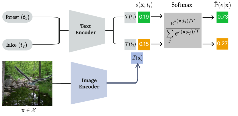
Figure 4: Illustration of zeros-shot group labeling using CLIP (Radford et al. 2021). The input image $\mathbf{x}$ is sampled from Waterbirds (Sagawa et al. 2020a). We calculate cosine similarity, $s(\mathbf{x};t_{i})$ between each text prompt $t_{i}$ and input image $\mathbf{x}$ in the embedding space. Finally, we calculate $\hat{\mathbb{P}}(e|\mathbf{x})$ by normalizing the cosine similarities with a softmax function.

Method	Dataset with group label	Waterbirds		CelebA
		Avg. Acc	Worst Group Acc	Avg. Acc	Worst Group Acc
G-DRO (Sagawa et al. 2020a)	train & val. set	92.4±0.2	90.7±0.9	92.8±0.3	88.7±1.5
PG-DRO (Ours)	5% val. set	91.7±0.2	89.2±0.5	92.0±0.3	89.4±1.0
PG-DRO (w/ CLIP) (Ours)	None	91.5±0.2	89.4±0.6	92.7±0.2	88.8±0.9

Table 5: Comparison of average and worst group test accuracies between methods leveraging CLIP model for pseudo labeling and those using supervised learning. Results (mean and std) of our proposed methods are estimated over 3 random seeds. Best performing results (among methods not using training set group annotations) are marked in bold.

Results.

In Table 5, we tabulate the performance of PG-DRO using zero-shot group labeling. We use PG-DRO (w/ CLIP) to differentiate approaches based on CLIP (as opposed to the default version in Section 3). We can draw two salient observations: (1) Zero-shot group labeling is fully compatible with our robust training objective and favorably matches the performance of G-DRO, which requires both training and validation sets. This is encouraging given there is no hand-annotated group labeling required in our approach. (2) PG-DRO (w/ CLIP) outperforms PG-DRO on both Waterbirds and CelebA datasets. Fundamentally, our method here differs from PG-DRO only in the pseudo-labeling technique. The improvement in worst-group test accuracy validates the efficacy of zero-shot group labeling.

Appendix B Training Details

In this section, we provide additional details on hyperparameter tuning for both pseudo labeling and robust training.

Pseudo labeling using supervised learning.

The configurations used for pseudo group labeling are summarized in Table 6. For CivilComments-WILDS dataset, we capped the number of tokens per example at 300.

Dataset	Optimizer	Learning Rate ($lr$)	$l_{2}$ penalty	Epochs	Batch Size
Waterbirds (Sagawa et al. 2020a)	SGD	$10^{-3}$	$10^{-4}$	200	64/16
CelebA (Liu et al. 2015)	SGD	$10^{-4}$	0.1	300	64
MultiNLI (Williams, Nangia, and Bowman 2018)	ADAMW	$2\times 10^{-5}$	0	50	32
CivilComments (Borkan et al. 2019; Koh et al. 2021)	ADAMW	$10^{-5}$	0.01	50	8

Table 6: Hyperparameter configurations used during pseudo labeling. To distinguish between configurations used when assuming group labeled annotations for whole validation set and $5\%$ of validation set, we use ‘val. set / 5% val. set’.

Robust training.

During robust training with PG-DRO, we perform the following hyperparameter sweeps:

• Vision Datasets. For both image classification tasks, Waterbirds (Sagawa et al. 2020a) and CelebA (Liu et al. 2015), we search the learning rate ($lr$) from {$10^{-3}$, $10^{-4}$, $10^{-5}$} and $l_{2}$ penalty from {1, 0.1, $10^{-4}$}. The generalization adjustment parameter $C$ is tuned over $\{0,1,2,3,4,5\}$ for both datasets.

• NLP Datasets. For MultiNLI (Williams, Nangia, and Bowman 2018), we directly use the hyperparameter values reported in (Sagawa et al. 2020a). For CivilComments-WILDS (Borkan et al. 2019; Koh et al. 2021) we use the same configuration as used in the pseudo labeling phase except using batch size 16. Similar to vision datasets, we tune $C$ over $\{0,1,2,3,4,5\}$ for both datasets.

We tabulate the best configurations for robust training in Table 7.

Dataset	Optimizer	Learning Rate ($lr$)	$l_{2}$ penalty	Epochs	Batch Size	$C$
Waterbirds (Sagawa et al. 2020a)	SGD	$10^{-5}$	1	300	128	2/4
CelebA (Liu et al. 2015)	SGD	$10^{-5}$	0.1	50	128	1/3
MultiNLI (Williams, Nangia, and Bowman 2018)	ADAMW	$2\times 10^{-5}$	0	10	32	1
CivilComments (Borkan et al. 2019; Koh et al. 2021)	ADAMW	$10^{-5}$	0.01	5	16	0

Table 7: Detailed hyperparameter configurations used during robust training. To distinguish between configurations used when assuming group labeled annotations for whole validation set and $5\%$ of validation set, we use ‘val. set / 5% val. set’

Appendix C Ablations on Adjustment Parameter

In this section, we perform experiments to ablate on generalization adjustment parameter $C$ in Equation 3. Specifically, in Figure 5, we report average and worst-group test accuracies on Waterbirds (Sagawa et al. 2020a) (left) and CelebA (Liu et al. 2015) (right) for different values of $C$.

We observe that for the Waterbirds dataset, using the generalization adjustment term provides a significant improvement in worst group test accuracy. Specifically, we see a 5.1% increase in worst group accuracy using $C=2$ as compared to not using the adjustment parameter ($C=0$). Setting a high value of $C$ may result in under-fitting the majority groups, thereby negatively impacting worst-group accuracy.

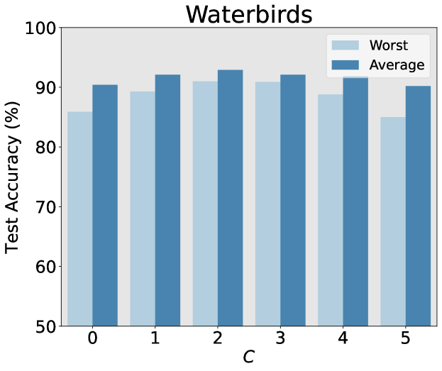
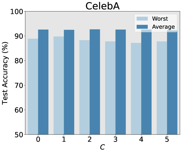
Figure 5: Ablations on the generalization adjustment parameter $C$ for Waterbirds (Sagawa et al. 2020a) (left) and CelebA (Liu et al. 2015) (right). We observe that using an tuned value of adjustment parameter $C$ provides boost to the worst-group accuracy for both datasets.

Appendix D Comparing Different Pseudo-labeling Techniques

In this section, we provide a brief comparison between two pseudo labeling approaches, based on: (1) Supervised learning (Nam et al. 2022), and (2) Zero-shot group classification using the large-scale pre-trained CLIP (Radford et al. 2021) model.

In Table 8, we report group-wise accuracies for each pseudo labeling technique on Waterbirds (Sagawa et al. 2020a). For evaluation, we compare the predicted group (with maximum confidence) vs. the hard group annotation.

On CelebA (Liu et al. 2015), we observe that group-wise accuracy using CLIP is on par with the semi-supervised learning approach despite being completely group-annotation-free. Considering Waterbirds (Sagawa et al. 2020a), we see that the CLIP model performs relatively poor for the under-represented group (waterbird on land). This can be attributed to the fact that ambiguity in the group membership for these samples is difficult to capture using simple text prompts, without using much prior information. However, using probabilistic group membership in such cases helps alleviate the problem.

Further, in Table 9 we tabulate the time required for both pseudo labeling techniques. For this benchmark, we run all experiments on a machine with 16 CPU cores and a single Nvidia Quadro RTX 5000 GPU. We can observe that being completely zero-shot, pseudo labeling using CLIP is much faster as compared to training using semi-supervised approaches.

Method	Dataset with group label	Land Bird		Water Bird
		Land	Water	Land	Water
Supervised	val. set	95.1	96.7	92.8	97.1
Supervised	5% val. set	89.4	94.1	96.4	90.7
Semi-Supervised (Nam et al. 2022)	val. set	94.7	96.2	92.8	96.4
Semi-Supervised (Nam et al. 2022)	5% val. set	83.7	95.1	91.1	93.3
Zero-shot(w/ CLIP)	None	97.3	88.6	83.9	98.3

Table 8: Comparison of group-wise accuracy of different pseudo-labeling technique, on the Waterbirds (Sagawa et al. 2020a) dataset. Accuracy for the most under-represented group is marked in bold.

Table 9: Runtime for each pseudo labeling technique for considered datasets.

Method	Waterbirds	CelebA	MultiNLI	CivilComments-WILDS
Semi-Supervised (Nam et al. 2022)	7.3 hrs	5.2 hrs	12.4 hrs	22.8 hrs
CLIP (Ours)	0.2 hr	0.6 hr	-	-

Appendix E Additional Results

E.1 GradCAM Visualizations

In Figure 7, we show GradCAM (Selvaraju et al. 2017) visualizations of few representative examples from Waterbirds (Sagawa et al. 2020a) dataset. Specifically, we compare models trained using SSA (Nam et al. 2022) and our proposed approach PG-DRO. For each input image, we show saliency maps where warmer colors depict higher saliency. We observe that PG-DRO consistently focuses on semantic regions representing essential cues for accurately identifying the foreground object such as claw, wing, beak, and fur. In contrast, the model trained using SSA (Nam et al. 2022) tends to output higher salience for spurious background attribute pixels. Given that both SSA (Nam et al. 2022) and PG-DRO uses a similar pseudo-labeling technique, this comparison highlights the significance of using group probabilities rather than one-hot labeling,

E.2 Visualization of Learned Representations

In Figure 8, we visualize the learned representations of test samples for models trained using ERM, SSA (Nam et al. 2022), G-DRO (Sagawa et al. 2020a) and our proposed framework PG-DRO. For each method, we show two UMAP plots. Specifically, we color each data point based on (1) spurious environment ($\mathcal{E}$) (top) and (2) true class label ($\mathcal{Y}$) (bottom). We observe that the model trained using ERM is highly dependent on environmental features for its prediction, signifying low worst group accuracy. Compared to ERM, both SSA and PG-DRO learns representations with more separability by $\mathcal{Y}$ as compared to $\mathcal{E}$.

Appendix F Software and Hardware

We run all experiments with Python 3.7.4 and PyTorch 1.9.0. For Waterbirds (Sagawa et al. 2020a) and CivilComments (Borkan et al. 2019; Koh et al. 2021), we use Nvidia Quadro RTX 5000 GPU. Experiments on CelebA (Liu et al. 2015) and MultiNLI (Williams, Nangia, and Bowman 2018) are run on a Google cloud instance with 12 CPUs and one Nvidia Tesla A100 GPU.

Table 10: Comparison of average and worst-group test accuracies for combinations of different group labeling approach and robust training methods when evaluated on image classification datasets: Waterbirds (Sagawa et al. 2020a) & CelebA (Liu et al. 2015). Results (mean and std) of our proposed methods are estimated over 3 random seeds for consistency.

Method	Dataset with group label	Waterbirds		CelebA
		Avg. Acc.	Worst Group Acc.	Avg. Acc.	Worst Group Acc.
ERM	None	97.3	63.2	95.6	47.2
G-DRO (Sagawa et al. 2020a)	train & val. set	92.4±0.2	90.7±0.9	92.8±0.3	88.7±1.5
SSA	val. set	92.2±0.9	89.0±0.6	92.8±0.1	89.8±1.3
PG-DRO (Ours)	val. set	92.4±0.4	91.0±0.8	92.5±0.3	89.8±1.1
SSA	$5\%$ of val. set	92.6±0.1	87.1±0.7	92.8±0.3	86.7±1.1
PG-DRO (Ours)	$5\%$ of val. set	91.9±0.2	89.2±0.6	91.7±0.3	87.8±1.0

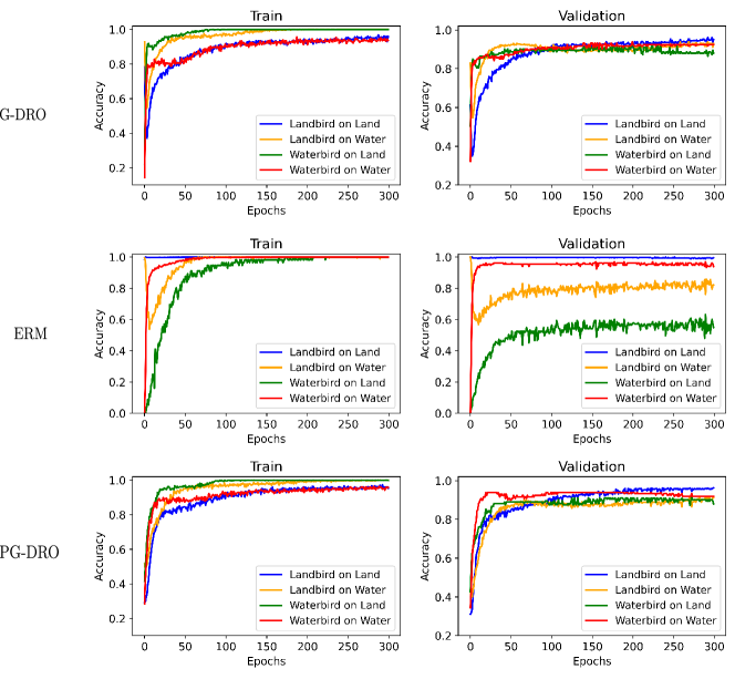
Figure 6: Training and validation accuracies for ERM, G-DRO and PG-DRO on Waterbirds (Sagawa et al. 2020a) dataset. As expected ERM trained model achieves perfect training accuracy across groups, but fails to generalize on worst-case group (waterbird on land).

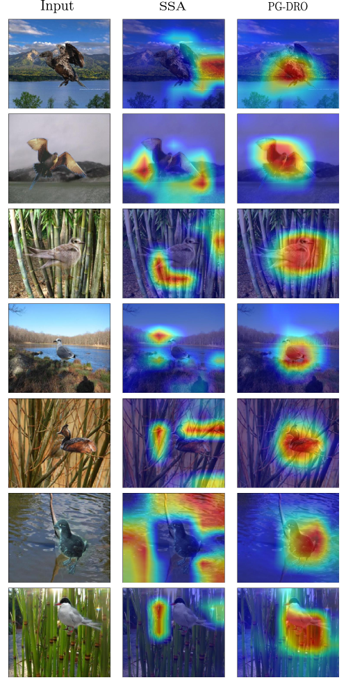
Figure 7: GradCAM visualizations for few images sampled from Waterbirds dataset (Sagawa et al. 2020a). We use GradCAM (Selvaraju et al. 2017) to visualize the “salient” observed features used to classify images.

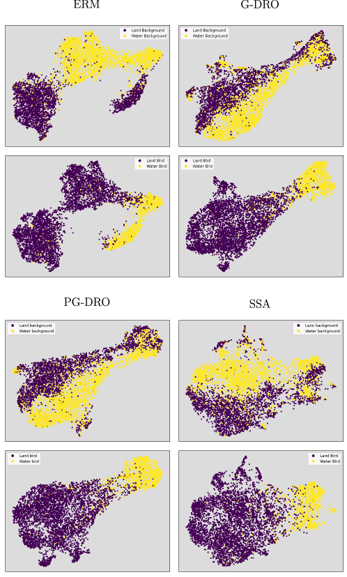
Figure 8: UMAP visualizations of learned representations for Waterbirds (Sagawa et al. 2020a) dataset. Specifically, we compare ERM, G-DRO (Sagawa et al. 2020a) and SSA (Nam et al. 2022) with our proposed approach PG-DRO. We color each data point based on (1) spurious environment ($\mathcal{E}$) (top) and (2) true class label ($\mathcal{Y}$) (bottom).

References

- Ben-Tal et al. (2013) Ben-Tal, A.; Den Hertog, D.; De Waegenaere, A.; Melenberg, B.; and Rennen, G. 2013. Robust solutions of optimization problems affected by uncertain probabilities. Management Science, 341–357.
- Bertsimas, Gupta, and Kallus (2018) Bertsimas, D.; Gupta, V.; and Kallus, N. 2018. Data-driven robust optimization. Mathematical Programming, 235–292.
- Blanchet and Murthy (2019) Blanchet, J.; and Murthy, K. 2019. Quantifying distributional model risk via optimal transport. Mathematics of Operations Research, 565–600.
- Borkan et al. (2019) Borkan, D.; Dixon, L.; Sorensen, J.; Thain, N.; and Vasserman, L. 2019. Nuanced Metrics for Measuring Unintended Bias with Real Data for Text Classification. In Companion Proceedings of The 2019 World Wide Web Conference, 491–500.
- Buolamwini and Gebru (2018) Buolamwini, J.; and Gebru, T. 2018. Gender shades: Intersectional accuracy disparities in commercial gender classification. In Conference on fairness, accountability and transparency, 77–91. PMLR.
- Byrd and Lipton (2019) Byrd, J.; and Lipton, Z. 2019. What is the effect of importance weighting in deep learning? In International Conference on Machine Learning, 872–881. PMLR.
- Creager, Jacobsen, and Zemel (2021) Creager, E.; Jacobsen, J.-H.; and Zemel, R. 2021. Environment inference for invariant learning. In International Conference on Machine Learning, 2189–2200. PMLR.
- Devlin et al. (2019) Devlin, J.; Chang, M.-W.; Lee, K.; and Toutanova, K. 2019. Bert: Pre-training of deep bidirectional transformers for language understanding. In Proceedings of NAACL-HLT, 4171–4186.
- Dosovitskiy et al. (2021) Dosovitskiy, A.; Beyer, L.; Kolesnikov, A.; Weissenborn, D.; Zhai, X.; Unterthiner, T.; Dehghani, M.; Minderer, M.; Heigold, G.; Gelly, S.; Uszkoreit, J.; and Houlsby, N. 2021. An Image is Worth 16x16 Words: Transformers for Image Recognition at Scale. In International Conference on Learning Representations.
- Geirhos et al. (2019) Geirhos, R.; Rubisch, P.; Michaelis, C.; Bethge, M.; Wichmann, F. A.; and Brendel, W. 2019. ImageNet-trained CNNs are biased towards texture; increasing shape bias improves accuracy and robustness. In International Conference on Learning Representations.
- Goel et al. (2021) Goel, K.; Gu, A.; Li, Y.; and Ré, C. 2021. Model Patching: Closing the Subgroup Performance Gap with Data Augmentation. In International Conference on Learning Representations.
- Gururangan et al. (2018) Gururangan, S.; Swayamdipta, S.; Levy, O.; Schwartz, R.; Bowman, S.; and Smith, N. A. 2018. Annotation Artifacts in Natural Language Inference Data. In Proceedings of the 2018 Conference of the North American Chapter of the Association for Computational Linguistics: Human Language Technologies, Volume 2 (Short Papers).
- He et al. (2016) He, K.; Zhang, X.; Ren, S.; and Sun, J. 2016. Deep residual learning for image recognition. In Proceedings of the IEEE/CVF Conference on Computer Vision and Pattern Recognition.
- Koh et al. (2021) Koh, P. W.; Sagawa, S.; Marklund, H.; Xie, S. M.; Zhang, M.; Balsubramani, A.; Hu, W.; Yasunaga, M.; Phillips, R. L.; Gao, I.; et al. 2021. Wilds: A benchmark of in-the-wild distribution shifts. In International Conference on Machine Learning, 5637–5664. PMLR.
- Lam and Zhou (2015) Lam, H.; and Zhou, E. 2015. Quantifying uncertainty in sample average approximation. In 2015 Winter Simulation Conference (WSC), 3846–3857. IEEE.
- Lee et al. (2013) Lee, D.-H.; et al. 2013. Pseudo-label: The simple and efficient semi-supervised learning method for deep neural networks. In Workshop on challenges in representation learning, ICML, 896.
- Levy et al. (2020) Levy, D.; Carmon, Y.; Duchi, J. C.; and Sidford, A. 2020. Large-scale methods for distributionally robust optimization. Advances in Neural Information Processing Systems.
- Liu et al. (2021) Liu, E. Z.; Haghgoo, B.; Chen, A. S.; Raghunathan, A.; Koh, P. W.; Sagawa, S.; Liang, P.; and Finn, C. 2021. Just train twice: Improving group robustness without training group information. In International Conference on Machine Learning, 6781–6792. PMLR.
- Liu et al. (2015) Liu, Z.; Luo, P.; Wang, X.; and Tang, X. 2015. Deep learning face attributes in the wild. In Proceedings of the IEEE/CVF International Conference on Computer Vision, 3730–3738.
- Mohajerin Esfahani and Kuhn (2018) Mohajerin Esfahani, P.; and Kuhn, D. 2018. Data-driven distributionally robust optimization using the Wasserstein metric: Performance guarantees and tractable reformulations. Mathematical Programming, 115–166.
- Mohri, Sivek, and Suresh (2019) Mohri, M.; Sivek, G.; and Suresh, A. T. 2019. Agnostic federated learning. In International Conference on Machine Learning, 4615–4625. PMLR.
- Nam et al. (2020) Nam, J.; Cha, H.; Ahn, S.; Lee, J.; and Shin, J. 2020. Learning from failure: De-biasing classifier from biased classifier. Advances in Neural Information Processing Systems.
- Nam et al. (2022) Nam, J.; Kim, J.; Lee, J.; and Shin, J. 2022. Spread Spurious Attribute: Improving Worst-group Accuracy with Spurious Attribute Estimation. In International Conference on Learning Representations.
- Namkoong and Duchi (2017) Namkoong, H.; and Duchi, J. C. 2017. Variance-based regularization with convex objectives. Advances in neural information processing systems.
- Oakden-Rayner et al. (2020) Oakden-Rayner, L.; Dunnmon, J.; Carneiro, G.; and Ré, C. 2020. Hidden stratification causes clinically meaningful failures in machine learning for medical imaging. In Proceedings of the ACM conference on health, inference, and learning, 151–159.
- Radford et al. (2021) Radford, A.; Kim, J. W.; Hallacy, C.; Ramesh, A.; Goh, G.; Agarwal, S.; Sastry, G.; Askell, A.; Mishkin, P.; Clark, J.; et al. 2021. Learning transferable visual models from natural language supervision. In International Conference on Machine Learning, 8748–8763. PMLR.
- Ren et al. (2018) Ren, M.; Zeng, W.; Yang, B.; and Urtasun, R. 2018. Learning to reweight examples for robust deep learning. In International conference on machine learning, 4334–4343. PMLR.
- Sagawa et al. (2020a) Sagawa, S.; Koh, P. W.; Hashimoto, T. B.; and Liang, P. 2020a. Distributionally robust neural networks for group shifts: On the importance of regularization for worst-case generalization. In International Conference on Learning Representations (ICLR).
- Sagawa et al. (2020b) Sagawa, S.; Raghunathan, A.; Koh, P. W.; and Liang, P. 2020b. An investigation of why overparameterization exacerbates spurious correlations. In International Conference on Machine Learning, 8346–8356. PMLR.
- Selvaraju et al. (2017) Selvaraju, R. R.; Cogswell, M.; Das, A.; Vedantam, R.; Parikh, D.; and Batra, D. 2017. Grad-CAM: Visual Explanations from Deep Networks via Gradient-Based Localization. In 2017 IEEE International Conference on Computer Vision (ICCV), 618–626.
- Shimodaira (2000) Shimodaira, H. 2000. Improving predictive inference under covariate shift by weighting the log-likelihood function. Journal of statistical planning and inference, 227–244.
- Shu et al. (2019) Shu, J.; Xie, Q.; Yi, L.; Zhao, Q.; Zhou, S.; Xu, Z.; and Meng, D. 2019. Meta-weight-net: Learning an explicit mapping for sample weighting. Advances in neural information processing systems.
- Sohoni et al. (2020) Sohoni, N.; Dunnmon, J.; Angus, G.; Gu, A.; and Ré, C. 2020. No subclass left behind: Fine-grained robustness in coarse-grained classification problems. Advances in Neural Information Processing Systems.
- Tu et al. (2020) Tu, L.; Lalwani, G.; Gella, S.; and He, H. 2020. An Empirical Study on Robustness to Spurious Correlations using Pre-trained Language Models. Transactions of the Association for Computational Linguistics, 621–633.
- Vapnik (1991) Vapnik, V. 1991. Principles of risk minimization for learning theory. Advances in neural information processing systems, 4.
- Vaswani et al. (2017) Vaswani, A.; Shazeer, N.; Parmar, N.; Uszkoreit, J.; Jones, L.; Gomez, A. N.; Kaiser, L.; and Polosukhin, I. 2017. Attention is All You Need. In Proceedings of the 31st International Conference on Neural Information Processing Systems, 6000–6010.
- Wah et al. (2011) Wah, C.; Branson, S.; Welinder, P.; Perona, P.; and Belongie, S. 2011. The Caltech-UCSD Birds-200-2011 Dataset. Technical Report CNS-TR-2011-001, California Institute of Technology.
- Wiesemann, Kuhn, and Sim (2014) Wiesemann, W.; Kuhn, D.; and Sim, M. 2014. Distributionally robust convex optimization. Operations Research, 1358–1376.
- Williams, Nangia, and Bowman (2018) Williams, A.; Nangia, N.; and Bowman, S. 2018. A Broad-Coverage Challenge Corpus for Sentence Understanding through Inference. In Proceedings of the 2018 Conference of the North American Chapter of the Association for Computational Linguistics: Human Language Technologies, Volume 1 (Long Papers), 1112–1122.
- Wolf et al. (2020) Wolf, T.; Debut, L.; Sanh, V.; Chaumond, J.; Delangue, C.; Moi, A.; Cistac, P.; Rault, T.; Louf, R.; Funtowicz, M.; Davison, J.; Shleifer, S.; von Platen, P.; Ma, C.; Jernite, Y.; Plu, J.; Xu, C.; Scao, T. L.; Gugger, S.; Drame, M.; Lhoest, Q.; and Rush, A. M. 2020. Transformers: State-of-the-Art Natural Language Processing. In Proceedings of the 2020 Conference on Empirical Methods in Natural Language Processing: System Demonstrations, 38–45.
- Zhang et al. (2020) Zhang, J.; Menon, A.; Veit, A.; Bhojanapalli, S.; Kumar, S.; and Sra, S. 2020. Coping with label shift via distributionally robust optimisation. arXiv preprint arXiv:2010.12230.
- Zhang et al. (2022) Zhang, M.; Sohoni, N. S.; Zhang, H. R.; Finn, C.; and Ré, C. 2022. Correct-N-Contrast: A Contrastive Approach for Improving Robustness to Spurious Correlations. arXiv preprint arXiv:2203.01517.
- Zhou et al. (2017) Zhou, B.; Lapedriza, A.; Khosla, A.; Oliva, A.; and Torralba, A. 2017. Places: A 10 million image database for scene recognition. IEEE transactions on pattern analysis and machine intelligence, 1452–1464.
- Zhu et al. (2017) Zhu, J.-Y.; Park, T.; Isola, P.; and Efros, A. A. 2017. Unpaired Image-to-Image Translation using Cycle-Consistent Adversarial Networks. In Computer Vision (ICCV), 2017 IEEE International Conference on.