On Hybrid Radar Fusion for Integrated Sensing and Communication

Abstract

The following paper introduces a novel integrated sensing and communication (ISAC) scenario termed hybrid radar fusion. In this setting, the dual-functional radar and communications (DFRC) base station (BS) acts as a mono-static radar in the downlink (DL), for sensing purposes, while performing its DL communication tasks. Meanwhile, the communication users act as distributed bi-static radar nodes in the uplink (UL) following a frequency-division duplex protocol. The DFRC BS fuses the information available at different DL and UL resource bands to estimate the angles-of-arrival (AoAs) of the multiple targets existing in the scene. In this work, we derive the maximum likelihood (ML) criterion for the hybrid radar fusion problem at hand. Additionally, we design efficient estimators; the first algorithm is based on an alternating optimization approach to solve the ML criterion, while the second one designs an optimization framework that leads to an alternating subspace approach to estimate AoAs for both the target and users. Finally, we demonstrate the superior performance of both algorithms in different scenarios, and the gains offered by these proposed methods through numerical simulations.

I Introduction

Despite having numerous similarities in terms of signal processing and system design, radar sensing and wireless communication have been evolving individually for many years [1]. Interestingly, both radar and communication (R&C) systems have quite a number of signal processing features that can be shared in common, thus favoring their joint design [2, 3, 4, 5, 6]. Indeed, integrated sensing and communication (ISAC) can open the way for ground-breaking applications, for e.g., in the automotive sector [7], Internet of things (IoT), and robotics.

ISAC has been investigated for different scenarios and challenges, including holographic communications [8], dual-functional radar and communication (DFRC) [9], waveform design [10], unmanned aerial vehicle (UAV) [11], beamforming design [12], IoT [13], just to name a few. Due to the interoperability between the R&C sub-systems, ISAC has a variety of tangible benefits, such as spectrum efficiency [14], less expensive modem by unifying hardware and software resources across sensing and communication (S&C) tasks [7]. These advantages bring a significant number of difficulties and research issues that must be resolved, such as the trade-offs between high data rates and high-resolution sensing. One of the earliest appearances of ISAC was in the 60s [15], where S&C tasks share the same power, spectrum and resources. In particular, pulse interval modulation was used for radar pulses and communication was embedded in those pulses. Owing to advances in waveform design, beamforming, and sofware-defined radios (SDRs), ISAC has become a reality.
ISAC can be categorized into three categories, from a design perspective. A joint design approach aims at developing new waveforms intended for S&C, while offering tradeoffs between different key performance indicators (KPIs), such as data rates, capacity, energy for communications and probability of detection and Cramér-Rao bound (CRB) for radar sensing. For e.g., the work in [16] proposes a joint design of S&C waveforms with adjustable peak-to-average power ratio (PAPR), allowing trade-offs between radar performance, communication rate and PAPR. Moreover, another design is radar-centric ISAC, where a radar waveform is considered and communication information is inserted onto the radar waveform [17, 18, 19]. Finally, communication-centric ISAC takes a communication waveform, for example, orthogonal frequency-division multiplexing (OFDM), and estimates sensing parameters based on channel information probed in that waveform. Here sensing is an ”add-on”. DFRC is a design technique that integrates R&C functions using a common transmit/receive aperture [20]. For radar, there are two common settings for radar: mono-static, where transmit and receive units are co-located and bi-static, where the units are separated. In this paper, we propose a new scheme named hybrid radar fusion (HRF) that considers both mono-static and bi-static settings, where the base station (BS) acts as a mono-static radar and users act as distributed bi-static radars in the uplink (UL) following a frequency-division duplex (FDD) protocol.

I-A Literature Review

To unbolt the potential of sensing capabilities in ISAC systems, various lines of research work have been conducted in the literature. In particular, the paper in [21] exploits OFDM based waveforms in the downlink (DL) only, from a mono-static radar perspective, and performs delay and Doppler estimation via periodogram criterion, which is only optimal for a single target. In addition, [22] considers a bi-static setting, in which S&C tasks are performed in orthogonal sets of sub-carriers, where the sub-carriers allocated to sensing are distributed among antennas in an interleaved fashion. Besides, the paper in [23] proposes an ISAC multi-user intelligent reflecting surface (IRS)-aided scheme, capable of carrying out UL data communications, while simultaneously performing target localization. Nevertheless, [24] investigates multi-beam systems for ISAC for 5G- new radio (NR) using OFDM waveforms. The BS in this study is a mono-static one, and joint range and angle of arrival (AoA) estimation are modeled as sensing parameters, which further assists the beam-scanning procedure. However, the framework utilizes only the DL information, and therefore the UL information available from different users is neglected. Meanwhile, [12, 25] consider the joint design of beamforming for S&C purposes, which is well-suited for beam-scanning applications. These frameworks also rely on DL-only communication information for sensing purposes. Furthermore, from a physical-layer security ISAC perspective, the work in [26] provides sensing estimation based on the eavesdropper location to improve the secrecy rate of the system. In short, the framework utilizes DL-only information for the radar echo. To the best of our knowledge, there does not exist any ISAC scheme in the literature that functions on a hybrid monostatic and bistatic mode and fuses UL and DL information to efficiently estimate target sensing parameters. The work in [27] focuses on a massive multiple-input, multiple-output (MIMO) ISAC setting where the S&C channels reveal joint sparsity. It is worth highlighting that, in contrast to the approach discussed in [27], our methodology does not rely on a massive MIMO setting, nor does it require a large number of antennas. In addition, we do operate under the assumption of a FDD communication protocol, where the DFRC BS further fuses channel estimates, hence, maximizing their utility for sensing purposes. From an estimation perspective, and in order to capture the joint sparse burst structure of the scattering components for sensing, the work in [27] employs a Turbo sparse bayesian learning algorithm, which shows promising results. However, it was assumed that the discrete AoA grid points for the dictionary (design) matrix should be set equal to the number of BS antennas to provide a good trade-off between AoA estimation and complexity. Consequently, achieving good performance necessitates a large number of antennas, presenting an advantageous prospect for massive MIMO applications. Additionally, the work in [28] proposes a compressed sensing for sensing purposes, in an ISAC massive MIMO setting.

I-B Contributions

In this paper, we propose a HRF system model, that combines both monostatic and bistatic modes, where the DFRC BS exploits the echos due to the DL communication signals, in conjunction with UL signals from a set of users associated with the DFRC BS. Each communication user transmits OFDM waveforms on its own resource band, where the DFRC BS then fuses the information from different resources to estimate angles of arrival (AoAs) of the targets in the scene. Since we propose to estimate sensing parameters of targets without evaluating communication performance, the considered system falls under the communication-assisted sensing category. In other terms, our main interest lies in the estimation quality of target AoAs with the aid of a well-established communication infrastructure. To this end, we outline our contributions as

• Hybrid Radar Model. We coin the term hybrid because of the diverse and distributed radar functionality considered in this paper, i.e. the DL echo is associated with a mono-static radar setting, as the DFRC’s transmit and receive units are assumed to be colocated. Meanwhile, a (user,DFRC) couple is seen as a bi-static radar, as the user is seen as a radar transmit unit in the UL, transmitting via an FDD protocol through OFDM communication signals, and the DFRC receive unit is the radar receiver. The DFRC’s sophisticated task is to fuse the hybrid data at its disposal to estimate target locations. To the best of our knowledge, the estimation model that arises due to the hybrid nature appears in the literature for the first time.

• Fused Maximum Likelihood Criterion. We derive the maximum likelihood (ML) criterion of the hybrid radar model, and highlight our interpretations, such as its resemblance with the classical ML criterion and the additional terms due to the participation of the communication users in the UL.

• Fused and Efficient Estimators. In light of the hybrid and dual nature of the available data, we propose two computationally attractive estimators. The first one explicitly tackles the ML criterion through an iterative optimization procedure that alternates between the target and user spaces. The second is an iterative subspace estimator: inspired by the multiple signal classification (MUSIC) principle, we formulate novel optimization problems, which lead to a new iterative estimator that carefully projects and fuses target and user location estimates.

• Extensive simulation results. Various performance metrics evaluating sensing performance via OFDM communication waveforms are studied through simulations, demonstrating the effectiveness of utilizing fused data for the hybrid radar model. Numerical results show performance gains in terms of mean squared error (MSE) of the estimated AoAs for the targets, especially when more communication users participate in the UL.

Notation: Upper-case and lower-case boldface letters denote matrices and vectors, respectively. $(.)^{T}$, $(.)^{*}$ and $(.)^{H}$ represent the transpose, the conjugate and the transpose-conjugate operators. The empty set is $\emptyset$. The cardinality of $\mathcal{C}$ is $|\mathcal{C}|$. The set of all complex-valued $N\times M$ matrices is $\mathbb{C}^{N\times M}$. The determinant is $\det()$. The trace is $\operatorname{tr}()$. The $N\times N$ identity matrix is $\boldsymbol{I}_{N}$. The projector operator onto the space spanned by columns of $\boldsymbol{A}\in\mathbb{C}^{N\times M}$ is $\boldsymbol{P}_{\boldsymbol{A}}$ and the corresponding orthogonal projector is $\boldsymbol{P}_{\boldsymbol{A}}^{\perp}\triangleq\boldsymbol{I}_{N}-\boldsymbol{P}_{\boldsymbol{A}}$. We index the $(i,j)^{th}$ element of $\boldsymbol{A}$ as $\boldsymbol{A}(i,j)$. The $k^{th}$ column of $\boldsymbol{A}$ is indexed as $\boldsymbol{A}(:,k)$. The $\operatorname{span}$ of $\boldsymbol{A}$, denoted $\operatorname{span}(\boldsymbol{A})$ returns the column space of $\boldsymbol{A}$. The Moore-Penrose pseudo-inverse of $\boldsymbol{A}$ is $\boldsymbol{A}^{+}$.

II System Model

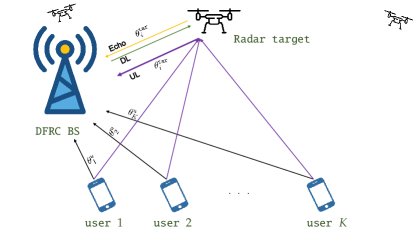
Figure 1: The HRF system model comprised of a DFRC BS in mono-static mode listening to its DL echo, with $K$ communication UL users and a radar target. We only depict one target due to illustration purposes.

Consider a DFRC BS transmitting OFDM symbols over its allocated band. The DFRC BS is equipped with $N_{t}$ transmit antennas aiding in S&C directional beamforming. Furthermore, assume that $q$ targets are present in the scene, where the $i^{th}$ target is located at $\theta_{i}^{\tt{tar}}$ from the DFRC BS. We denote this set as $\boldsymbol{\Theta}^{\tt{tar}}=\begin{bmatrix}\theta_{1}^{\tt{tar}}&\ldots&\theta_{q}^{\tt{tar}}\end{bmatrix}$. In the DL, the $\ell^{th}$ transmitted OFDM signal can be expressed as

$$\boldsymbol{s}_{0,\ell}(t)=\Big{(}\sum\nolimits_{m\in\mathcal{C}_{0}}b_{m,0}^{(\ell)}\exp(j2\pi m\Delta_{f}t)\Pi(t-\ell T)\Big{)}\boldsymbol{f},$$ (1)

where $\boldsymbol{f}\in\mathcal{C}^{N_{t}\times 1}$ is the transmit beamforming vector. Furthermore, $\mathcal{C}_{0}$ is the set of subcarriers corresponding to the allocated band in the DL. Furthermore, $b_{m,0}^{(\ell)}$ is the symbol on the $m^{th}$ OFDM subcarrier within the $\ell^{th}$ OFDM symbol and $\Delta_{f}$ is the subcarrier spacing. Also, the number of OFDM symbols in the DL is denoted as $L_{0}$. Moreover, the OFDM symbol duration is given $T=\frac{1}{\Delta_{f}}$. Also, $\Pi(t)$ is a certain windowing function. The overall OFDM symbol duration is denoted as $T_{o}\triangleq T+T_{\text{CP}}$, where $T_{\text{CP}}$ is the cyclic prefix duration. Assuming the ideal rectangular function, the window function should satisfy $\Pi(t)=1$, if $t\in[-T_{\text{CP}},T]$, and $0$, else. Here, $T_{\text{CP}}$ should be greater than the maximum of propagation delays in order to guarantee a cyclic convolution with the channel. The $\ell^{th}$ transmitted OFDM symbol from the single-antenna $k^{th}$ user in the UL is given by

$$s_{k,\ell}(t)=\sum\nolimits_{m\in\mathcal{C}_{k}}b_{m,k}^{(\ell)}\exp(j2\pi m\Delta_{f}t)\Pi(t-\ell T),$$ (2)

where $\mathcal{C}_{k}$ is the set of subcarriers corresponding to the allocated band for the $k^{th}$ user in the UL. Moreover, $b_{m,k}^{(\ell)}$ is the symbol on the $m^{th}$ OFDM subcarrier by the $k^{th}$ user within the $\ell^{th}$ OFDM symbol. Also, the transmission consists of $L_{k}$ OFDM symbols for the $k^{th}$ user. We have that $\mathcal{C}_{0}\cup\mathcal{C}_{1}\cup\ldots\cup\mathcal{C}_{K}=\{0,1,\ldots,M-1\}$, where $M$ is the total number of subcarriers occupied by the entire system, i.e. the total occupied bandwidth is $M\Delta_{f}$. We also assume that the subcarrier sets are non-overlapping, i.e. $\mathcal{C}_{i}\cap\mathcal{C}_{j}=\emptyset$ for all $i\neq j$. Assuming a colocated mono-static MIMO radar setting, the time-domain baseband channel at a given time $t$ and at the $n^{th}$ receive antenna can be represented as follows

$$\boldsymbol{h}_{n}^{\tt{echo}}(t)=\sum\nolimits_{i\in\Phi_{0}}g_{i}^{\tt{tar}}a_{n}(\theta_{i}^{\tt{tar}})\boldsymbol{a}_{t}^{T}(\theta_{i}^{\tt{tar}})\delta(t-2\tau_{i}^{\tt{tar}})e^{j2\pi f_{D,i}t},$$ (3)

where $\Phi_{0}$ denotes the set of target indices explored by the DFRC BS. The time of arrival (ToA) between the DFRC BS and the $i^{th}$ target is denoted as $\tau_{i}^{\tt{tar}}$. The frequency $f_{D,i}$ represents the Doppler frequency of the $i^{th}$ target, which arises due to the movement of the target. The vector $\boldsymbol{a}_{t}(\theta)\in\mathbb{C}^{N_{t}\times 1}$ is the transmit steering vector pointing towards angle of departure (AoD) $\theta$. Notice that due to the mono-static configuration, the AoA and AoD of a certain target are the same. The general expression of the steering response of the $n^{th}$ antenna due to a signal arriving at angle $\theta$, $a_{n}(\theta)$, is generally dependent on the frequency. Its most general form follows

$$a_{n}(\theta,f)=\exp\Big{(}j2\pi\frac{f}{c}(x_{n}\sin(\theta)+y_{n}\cos(\theta))\Big{)},$$ (4)

where $(x_{n},y_{n})$ represent the cartesian coordinates of antenna $n$ in the $(x,y)-$ plane and $\theta$ is the AoA. In this paper, we follow a narrowband assumption, i.e. the bandwidth occupied by the FDD protocol, $B=\sum_{k=0}^{K}|\mathcal{C}_{k}|\Delta_{f}$ is much smaller than the carrier frequency $f_{c}$, i.e. $\frac{B}{2f_{c}}\ll 1$. Hence, $a_{n}(\theta,f)\simeq a_{n}(\theta)=\exp\big{(}j2\pi\frac{f_{c}}{c}(x_{n}\sin(\theta)+y_{n}\cos(\theta))\big{)}$. A similar discussion can be done on the transmit steering vector $\boldsymbol{a}_{t}(\theta)$. The term $g_{i}^{\tt{tar}}$ is the two-way propagation complex gain of the $i^{th}$ target which also contains an initial phase offset. Its magnitude is given by the two-way path-loss equation as

$$|g_{i}^{\tt{tar}}|=\sqrt{\frac{\lambda^{2}\sigma^{{\tt{RCS}}}_{i}\beta_{\tt{Tx}}(\theta_{i}^{\tt{tar}})\beta_{\tt{Rx}}(\theta_{i}^{\tt{tar}})}{(4\pi)^{3}(d_{i}^{\tt{tar}})^{4}}},$$ (5)

where $\sigma^{{\tt{RCS}}}_{i}$ is the radar cross-section (RCS) of the $i^{th}$ target and $d_{i}^{\tt{tar}}$ is the Euclidean distance between the $i^{th}$ target and the DFRC BS. In fact, $\tau_{i}^{\tt{tar}}=\frac{d_{i}^{\tt{tar}}}{c}$, where $c$ is the speed of light. The terms $\beta_{\tt{Tx}}(\theta)$ and $\beta_{\tt{Rx}}(\theta)$ represent the gain of the transmit and receive antenna elements at look-direction $\theta$, respectively. The wavelength is $\lambda$. On the other hand, the UL channel between the $k^{th}$ communication user and the DFRC BS is characterized as follows

$$\begin{split}h_{n,k}^{\tt{UL}}(t)&=g_{0,k}^{\tt{u}}a_{n}(\theta_{k}^{\tt{u}})\delta(t-\tau_{k}^{\tt{u}})\\ &+\sum\nolimits_{i\in\Phi_{k}}g_{i,k}^{\tt{tar}}a_{n}(\theta_{i}^{\tt{tar}})\delta(t-\phi_{k,i})e^{j2\pi f_{D,i}t},\end{split}$$ (6)

where the first term is the line of sight (LoS) channel between the $k^{th}$ user and the DFRC BS. The second term constitutes the two-way channel between the $k^{th}$ user towards the set of targets $\Phi_{k}$, where $\Phi_{k}$ denotes the set of target indices explored by the $k^{th}$ user. The indices within $\Phi_{k}$ are denoted as $\Phi_{k}=\begin{bmatrix}u_{1}^{(k)},&\ldots,&u^{(k)}_{|\Phi_{k}|}\end{bmatrix}$, for all $k=0\ldots K$. Furthermore, we assume that the union of indices defined by the set of targets explored by the DFRC BS and all users cover all the $q$ targets, namely $\bigcup_{k}\Phi_{k}=\{1\ldots q\}$. In general, $|\Phi_{k}|\leq|\Phi_{0}|$ for $k=1,2,\cdots,K$, and $\Phi_{i}\neq\Phi_{j}$ for $i\neq j$. The AoA between the $k^{th}$ user and BS is $\theta_{k}^{\tt{u}}$. The path gains are given as

$$|g_{0,k}^{\tt{u}}| =\sqrt{\frac{\lambda^{2}\beta_{\tt{Tx}}^{\tt{u}}(\theta_{k}^{\tt{u}})\beta_{\tt{Rx}}(\theta_{k}^{\tt{u}})}{(4\pi)^{2}(d_{k}^{\tt{u}})^{2}}},$$ (7)

$$|g_{i,k}^{\tt{tar}}| =\sqrt{\frac{\lambda^{2}\bar{\sigma}^{{\tt{RCS}}}_{i,k}\beta_{\tt{Tx}}^{\tt{u}}(\psi_{k,i})\beta_{\tt{Rx}}(\theta_{i}^{\tt{tar}})}{(4\pi)^{3}(d_{k,i})^{2}(d_{i}^{\tt{tar}})^{2}}},$$ (8)

where $\beta_{\tt{Tx}}^{\tt{u}}(\theta)$ is the gain of the user’s antenna towards direction $\theta$, $\psi_{k,i}$ and $d_{k,i}$ represent the angle and distance between the $k^{th}$ user and the $i^{th}$ target, respectively. In addition, $\bar{\sigma}^{{\tt{RCS}}}_{i,k}$ is the RCS of the $i^{th}$ target due to the $k^{th}$ communication user. The term $d_{k}^{\tt{u}}$ is the distance between the $k^{th}$ user and the DFRC BS. In addition, we denote the ToA between the $k^{th}$ user and the DFRC BS as $\tau_{k}^{\tt{u}}=\frac{d_{k}^{\tt{u}}}{c}$. Also, the two-way delay $\phi_{k,i}$ is the delay from $k^{th}$ user towards $i^{th}$ target then towards the DFRC BS, i.e. $\phi_{k,i}=\frac{d_{k,i}+d_{i}^{\tt{tar}}}{c}=\tau_{k,i}+\tau^{\tt{tar}}_{i}$, and $\tau_{k,i}$ is the one-way delay between the $k^{th}$ user and $i^{th}$ target. The $\ell^{th}$ OFDM symbol at the $n^{th}$ receive antenna of the BS after performing convolution and downconversion can be written as

$$r_{n,\ell}(t)=r_{n,\ell}^{\tt{echo}}(t)+\sum\nolimits_{k=1}^{K}r_{n,\ell,k}^{\tt{UL}}(t)+w_{n,\ell}(t),$$ (9)

where $r_{n,\ell}^{\tt{echo}}(t)$ is the received echo signal due to the presence of the radar targets, i.e.

$$r_{n,\ell}^{\tt{echo}}(t)=\sum\nolimits_{i\in\Phi_{0}}\gamma_{i,\ell}^{\tt{tar}}(\boldsymbol{a}_{t}^{T}(\theta_{i}^{\tt{tar}})\boldsymbol{f})a_{n}(\theta_{i}^{\tt{tar}})s_{0,\ell}(t-2\tau_{i}^{\tt{tar}}).$$ (10)

Furthermore, $r_{n,\ell,k}^{\tt{UL}}(t)$ is the received signal due to the channel between the $k^{th}$ user and the DFRC BS, taking into account the direct LoS and bounces due to the presence of targets, i.e.

$$\begin{split}r_{n,\ell,k}^{\tt{UL}}(t)&=\gamma_{0,\ell,k}^{\tt{u}}a_{n}(\theta_{k}^{\tt{u}})s_{k,\ell}(t-\tau_{k}^{\tt{u}})\\ &+\sum\nolimits_{i\in\Phi_{k}}\gamma_{i,\ell,k}^{\tt{tar}}a_{n}(\theta_{i}^{\tt{tar}})s_{k,\ell}(t-\phi_{k,i}).\end{split}$$ (11)

In the above, we have approximated the varying phases due to Doppler frequency over an OFDM block symbol as constant [14], therefore, $\gamma_{i,\ell}^{\tt{tar}}=g_{i}^{\tt{tar}}e^{j2\pi\ell Tf_{D,i}}$. Likewise, $\gamma_{i,\ell,k}^{\tt{tar}}=g_{i,k}^{\tt{tar}}e^{j2\pi\ell Tf_{D,i}}$ and $\gamma_{0,\ell,k}^{\tt{u}}=g_{0,k}^{\tt{u}}$. The background noise in (9) is denoted as $w_{n,\ell}(t)$, which is assumed to be independently and identically distributed (i.i.d) additive white Gaussian noise (AWGN). Now, plugging equations (1) and (2) in equations (10) and (11), and sampling at regular intervals of $p\triangleq p\frac{T}{M}$, we can express equation (9) as follows

$$\begin{split}r_{n,\ell}[p]&=\sum\limits_{\begin{subarray}{c}i\in\Phi_{0}\\ m\in\mathcal{C}_{0}\end{subarray}}b_{m,0}^{(\ell)}e^{j2\pi\frac{mp}{M}}c_{m}(2\tau_{i}^{\tt{tar}})\gamma_{i,\ell}^{\tt{tar}}(\boldsymbol{a}_{t}^{T}(\theta_{i}^{\tt{tar}})\boldsymbol{f})a_{n}(\theta_{i}^{\tt{tar}})\\ &+\sum\limits_{\begin{subarray}{c}k=1\ldots K\\ m\in\mathcal{C}_{k}\end{subarray}}b_{m,k}^{(\ell)}e^{j2\pi\frac{mp}{M}}c_{m}(\tau_{k}^{\tt{u}})\gamma_{0,\ell,k}^{\tt{u}}a_{n}(\theta_{k}^{\tt{u}})\\ &+\sum\limits_{\begin{subarray}{c}k=1\ldots K\\ m\in\mathcal{C}_{k}\\ i\in\Phi_{k}\end{subarray}}b_{m,k}^{(\ell)}e^{j2\pi\frac{mp}{M}}c_{m}(\phi_{k,i})\gamma_{i,\ell,k}^{\tt{tar}}a_{n}(\theta_{i}^{\tt{tar}})+w_{n,\ell}[p],\end{split}$$ (12)

where $c_{m}(\tau)=e^{-j2\pi m\Delta_{f}\tau}$. Gathering $M$ time samples of $r_{n,\ell}[p]$ and performing a discrete Fourier transform (DFT), we have

$$R_{n,\ell,m}=\frac{1}{M}\sum\nolimits_{p=0}^{M-1}r_{n,\ell}[p]e^{-j2\pi\frac{mp}{M}}.$$ (13)

Due to the above DFT, and thanks to the orthogonality in frequency domain due to FDD operation, i.e. $\mathcal{C}_{i}\cap\mathcal{C}_{j}=\emptyset$ for all $i\neq j$, we have

$$Y_{n,\ell,m,k}=R_{n,\ell,m}\Big{|}_{m\in\mathcal{C}_{k}},\quad k=0\ldots K$$ (14)

where

$$\begin{split}Y_{n,\ell,m,0}&=\sum\nolimits_{i\in\Phi_{0}}c_{m}(2\tau_{i}^{\tt{tar}})\gamma_{i,\ell}^{\tt{tar}}(\boldsymbol{a}_{t}^{T}(\theta_{i}^{\tt{tar}})\boldsymbol{f})a_{n}(\theta_{i}^{\tt{tar}})\\ &+W_{n,\ell,m,0},\end{split}$$ (15)

for $m\in\mathcal{C}_{0}$, and

$$\begin{split}Y_{n,\ell,m,k}&=c_{m}(\tau_{k}^{\tt{u}})\gamma_{0,\ell,k}^{\tt{u}}a_{n}(\theta_{k}^{\tt{u}})\\ &+\sum\nolimits_{i\in\Phi_{k}}c_{m}(\phi_{k,i})\gamma_{i,\ell,k}^{\tt{tar}}a_{n}(\theta_{i}^{\tt{tar}})+W_{n,\ell,m,k},\end{split}$$ (16)

for $m\in\mathcal{C}_{k}$ for all $k\geq 1$. Without loss of generality, we have assumed that $b_{m,k}^{(\ell)}=1$, as those are known pilot symbols. Equations (15) and (16) are arranged, via matrix form, namely

$$\boldsymbol{Y}_{0} =\boldsymbol{A}(\boldsymbol{\Theta}^{\tt{tar}}_{0})\boldsymbol{X}_{0}+\boldsymbol{W}_{0},$$ (17)

$$\boldsymbol{Y}_{k} =\begin{bmatrix}\boldsymbol{a}(\theta_{k}^{\tt{u}})&\boldsymbol{A}(\boldsymbol{\Theta}^{\tt{tar}}_{k})\end{bmatrix}\boldsymbol{X}_{k}+\boldsymbol{W}_{k},\quad k=1\ldots K.$$ (18)

For UL communications, the preamble $s_{k,\ell}(t)$ is usually precedes a payload. The payload can be decoded by using the channel estimate per user, i.e. $Y_{n,\ell,m,k}$. Let $\mathcal{C}_{k}=\{p_{1},p_{2},\ldots,p_{|\mathcal{C}_{k}|}\}$ be the subcarrier indices occupied by the $k^{th}$ user in the UL. To this extent, we define $\boldsymbol{X}_{k}$ as

$$\boldsymbol{X}_{k}=\begin{bmatrix}\boldsymbol{x}_{1,p_{1}}^{(k)},\ldots,\boldsymbol{x}_{L_{k},p_{1}}^{(k)},\ldots,\boldsymbol{x}_{1,p_{|\mathcal{C}_{k}|}}^{(k)},\ldots,\boldsymbol{x}_{L_{k},p_{|\mathcal{C}_{k}|}}^{(k)}\end{bmatrix},$$ (19)

where $\boldsymbol{x}_{\ell,m}^{(k)}$ is a function of the gains, delays, as well as Doppler shifts. Generally speaking, the vector $\boldsymbol{x}_{\ell,m}^{(k)}$ can also be modeled to contain synchronization parameters caused by misalignment of oscillator clocks between the DFRC BS and the UL users, giving rise to time offsets and frequency offsets. Hence, these parameters may not have severe impact on the AoA estimation performance. In this paper, we treat variables $\boldsymbol{x}_{\ell,m}^{(k)}$ as nuisance parameters with arbitrary structure, allowing for its estimation and compensation at a following stage. Notice that $\boldsymbol{X}_{k}\in\mathbb{C}^{(|\Phi_{k}|+1)\times\bar{L}_{k}},\forall k=1\ldots K$ and $\bar{L}_{k}=L_{k}|\mathcal{C}_{k}|$ is the overall number of snapshots seen by the DFRC BS from the $k^{th}$ user in the UL. Likewise, $\boldsymbol{X}_{0}\in\mathbb{C}^{|\Phi_{0}|\times\bar{L}_{0}}$ and $\bar{L}_{0}$ is the total number of snapshots seen through the transmitted DL OFDM frame. Furthermore, the manifold matrix $\boldsymbol{A}(\boldsymbol{\Theta}^{\tt{tar}}_{k})$ is

$$\boldsymbol{A}(\boldsymbol{\Theta}^{\tt{tar}}_{k})=\begin{bmatrix}\boldsymbol{a}(\theta_{u^{(k)}_{1}}^{\tt{tar}})&\ldots&\boldsymbol{a}(\theta_{u^{(k)}_{|\Phi_{k}|}}^{\tt{tar}})\end{bmatrix}\in\mathbb{C}^{N\times|\Phi_{k}|},$$ (20)

and the steering vector is given by

$$\boldsymbol{a}(\theta)=\begin{bmatrix}\boldsymbol{a}_{1}(\theta)&\ldots&\boldsymbol{a}_{N}(\theta)\end{bmatrix}^{T}\in\mathbb{C}^{N\times 1}.$$ (21)

Moreover, the entries of $\boldsymbol{W}_{k}$ contain $W_{n,\ell,m,k}$ for $m\in\mathcal{C}_{k}$. In this paper, since we are interested in target AoA estimation, we shall treat the entries of $\boldsymbol{X}_{0},\boldsymbol{X}_{1}\ldots\boldsymbol{X}_{K}$ as nuisance parameters, as the estimation of complex channel gains, ToA and Doppler parameters is not the main focus herein.

Furthermore, observing equations (17) and (18), one can directly relate each equation to the classical AoA estimation problem. However, we would like to stress the fundamental difference between the AoA problem at hand and the classical one. Even though each of the $K+1$ matrix equations in (17) and (18) are classical AoA-type equations, the information contained over all equations is not. More specifically, each user over its occupied bandwidth, defined by $\mathcal{C}_{k}$, contains the manifold of interest $\boldsymbol{A}(\boldsymbol{\Theta}^{\tt{tar}}_{k})$ appended by an unknown channel $\boldsymbol{a}(\theta_{k}^{\tt{u}})$, linking the $k^{th}$ user towards the DFRC BS.

Our system model is illustrated in Fig. 1. We can see that the DFRC BS broadcasts the DL data and listens to the received echo at its allocated band. Meanwhile, the users each transmit OFDM symbols within their own band in the UL. Each communication contributes in two components:(i) a LoS path between itself and the DFRC BS, which is assumed to be unknown and (ii) the bounce from the target towards the DFRC BS within the users allocated band. The DFRC BS would then fuse the information available at all the bands, in order to estimate the unknown AoAs.

Before we introduce the estimation criteria and methods, we would like to take a moment and observe the joint model appearing in equations (17) and (18). The joint consideration of the $K+1$ models is the first time to be addressed, from an estimation perspective. Indeed, if we regard each of the $K+1$ models separately, then we coincide with a classical AoA estimation problem. However, the fused processing of all the $K+1$ models can be leveraged to our advantage, due to the presence of a common manifold being shared across all the bands, $\boldsymbol{A}(\boldsymbol{\Theta}^{\tt{tar}}_{\cap})$, where $\boldsymbol{\Theta}^{\tt{tar}}_{\cap}=\boldsymbol{\Theta}_{0}^{\tt{tar}}\cap\boldsymbol{\Theta}_{1}^{\tt{tar}}\cap\ldots\cap\boldsymbol{\Theta}_{K}^{\tt{tar}}$. To this end, we are ready to address our problem: by fusing the observations $\{\boldsymbol{Y}_{0},\boldsymbol{Y}_{1}\ldots\boldsymbol{Y}_{K}\}$ as defined in (17) and (18), we would like to estimate $\boldsymbol{\Theta}^{\tt{tar}}$, as well as $\boldsymbol{\Theta}^{\tt{u}}$.

III Fused Maximum Likelihood

In this section, we derive the deterministic ML for estimating $\boldsymbol{\Theta}^{\tt{tar}}$ and $\boldsymbol{\Theta}^{\tt{u}}$. The deterministic ML regards the sample functions as unknown deterministic sequences, rather than random processes. As shall be clarified, we can interpret our ML criterion as a fused maximum likelihood (FML) one. Denoting $\boldsymbol{Y}=\begin{bmatrix}\boldsymbol{Y}_{0}&\ldots&\boldsymbol{Y}_{K}\end{bmatrix}$, we express the joint density function of the observed data per allocated bandwidth as

$$\begin{split}f(\boldsymbol{Y})=&\prod_{k=0}^{K}\prod_{p=1}^{\bar{L}_{k}}\frac{1}{\pi\det(\sigma^{2}\boldsymbol{I})}\\ &\times\exp\Big{(}-\frac{1}{\sigma^{2}}\big{\|}\boldsymbol{Y}_{k}(:,p)-\boldsymbol{A}_{k}\boldsymbol{X}_{k}(:,p)\big{\|}^{2}\Big{)},\end{split}$$ (22)

where, for notation’s sake, we denote

$$\boldsymbol{A}_{k}=\begin{cases}\boldsymbol{A}(\boldsymbol{\Theta}^{\tt{tar}}_{0})&,k=0\\ \begin{bmatrix}\boldsymbol{a}(\theta_{k}^{\tt{u}})&\boldsymbol{A}(\boldsymbol{\Theta}^{\tt{tar}}_{k})\end{bmatrix}&,1\leq k\leq K.\end{cases}$$ (23)

Note that $f(\boldsymbol{Y})$ is conditioned over $\boldsymbol{X}_{0}\ldots\boldsymbol{X}_{K},\sigma^{2},\boldsymbol{\Theta}^{\tt{tar}},\boldsymbol{\Theta}^{\tt{u}}$, and this dependency has been omitted for sake of compact notation. Ignoring constant terms, the $\log$-likelihood function, $\mathcal{L}\triangleq\log f(\boldsymbol{Y})$, can be expressed as

$$\begin{split}\mathcal{L}\sim-N\bar{L}\log\sigma^{2}-\frac{1}{\sigma^{2}}\sum\nolimits_{p,k}\big{\|}\boldsymbol{Y}_{k}(:,p)-\boldsymbol{A}_{k}\boldsymbol{X}_{k}(:,p)\big{\|}^{2},\end{split}$$ (24)

where $\bar{L}=\sum_{k=0}^{K}\bar{L}_{k}$. The ML criterion is now given as

$$\big{\{}\widehat{\sigma}^{2},\widehat{\boldsymbol{X}},\widehat{\boldsymbol{\Theta}}^{\tt{tar}},\widehat{\boldsymbol{\Theta}}^{\tt{u}}\big{\}}=\operatorname*{arg\,max}\nolimits_{\{\sigma^{2},\boldsymbol{X},\boldsymbol{\Theta}^{\tt{tar}},\boldsymbol{\Theta}^{\tt{u}}\}}\mathcal{L}$$ (25)

where $\boldsymbol{X}=\begin{bmatrix}\boldsymbol{X}_{0}&\boldsymbol{X}_{1}&\ldots&\boldsymbol{X}_{K}\end{bmatrix}$. To proceed, we first carry out the maximization process over $\sigma^{2}$ by fixing $\boldsymbol{X},\boldsymbol{\Theta}^{\tt{tar}},\boldsymbol{\Theta}^{\tt{u}}$. This gives us

$$\widehat{\sigma}^{2}=\frac{1}{N\bar{L}}\sum\nolimits_{p,k}\big{\|}\boldsymbol{Y}_{k}(:,p)-\boldsymbol{A}_{k}\boldsymbol{X}_{k}(:,p)\big{\|}^{2}.$$ (26)

Replacing (26) back into the $\log$-likelihood function and ignoring constant terms again, we get

$$-N\bar{L}\log\Big{(}\frac{1}{N\bar{L}}\sum\nolimits_{k=0}^{K}\sum\nolimits_{p=1}^{\bar{L}_{k}}\big{\|}\boldsymbol{Y}_{k}(:,p)-\boldsymbol{A}_{k}\boldsymbol{X}_{k}(:,p)\big{\|}^{2}\Big{)}.$$ (27)

Using the monotonic property of the $\log$ function, the optimization criterion in (27) is now

$$\big{\{}\widehat{\boldsymbol{X}},\widehat{\boldsymbol{\Theta}}^{\tt{tar}},\widehat{\boldsymbol{\Theta}}^{\tt{u}}\big{\}}=\operatorname*{arg\,min}_{\{\boldsymbol{X},\boldsymbol{\Theta}^{\tt{tar}},\boldsymbol{\Theta}^{\tt{u}}\}}\sum\nolimits_{p,k}\big{\|}\boldsymbol{Y}_{k}(:,p)-\boldsymbol{A}_{k}\boldsymbol{X}_{k}(:,p)\big{\|}^{2}.$$ (28)

Now fixing $\boldsymbol{\Theta}^{\tt{tar}},\boldsymbol{\Theta}^{\tt{u}}$, the optimization with respect of $\boldsymbol{X}_{k}$ is the well known least squares (LS) over the $k^{th}$ user, i.e.

$$\widehat{\boldsymbol{X}}_{k}=\big{(}\boldsymbol{A}_{k}^{H}\boldsymbol{A}_{k}\big{)}^{-1}\boldsymbol{A}_{k}^{H}\boldsymbol{Y}_{k}.$$ (29)

Note that the estimator of $\boldsymbol{X}_{k}$ in (29) does not correspond to the exact ML. Instead, it corresponds to a relaxed version of ML by treating $\boldsymbol{X}_{k}$ as an arbitrary matrix instead of considering its special structure as per equations (15) and (16). Regarding $\boldsymbol{X}_{k}$ as a nuissance parameter comes with some benefits: First, we bypass the need of estimating gain, delay and Doppler parameters related to each user and target. Second, this assumption simplifies the complexity of the resulting ML estimator. Plugging (29) into (28), we get

$$\big{\{}\widehat{\boldsymbol{\Theta}}^{\tt{tar}},\widehat{\boldsymbol{\Theta}}^{\tt{u}}\big{\}}=\operatorname*{arg\,min}_{\{\boldsymbol{\Theta}^{\tt{tar}},\boldsymbol{\Theta}^{\tt{u}}\}}\sum\nolimits_{p,k}\big{\|}\boldsymbol{Y}_{k}(:,p)-\boldsymbol{P}_{k}\boldsymbol{Y}_{k}(:,p)\big{\|}^{2},$$ (30)

where $\boldsymbol{P}_{k}$ is the projector matrix projecting onto the column space of matrix $\boldsymbol{A}_{k}$, namely

$$\boldsymbol{P}_{k}=\boldsymbol{A}_{k}\big{(}\boldsymbol{A}_{k}^{H}\boldsymbol{A}_{k}\big{)}^{-1}\boldsymbol{A}_{k}^{H}.$$ (31)

The criterion in (30) can be replaced as

$$\big{\{}\widehat{\boldsymbol{\Theta}}^{\tt{tar}},\widehat{\boldsymbol{\Theta}}^{\tt{u}}\big{\}}=\operatorname*{arg\,max}_{\{\boldsymbol{\Theta}^{\tt{tar}},\boldsymbol{\Theta}^{\tt{u}}\}}\sum\nolimits_{p,k}\big{\|}\boldsymbol{P}_{k}\boldsymbol{Y}_{k}(:,p)\big{\|}^{2},$$ (32)

A more compact and convenient form to express the above ML cost is via the trace operator, i.e.

$$\big{\{}\widehat{\boldsymbol{\Theta}}^{\tt{tar}},\widehat{\boldsymbol{\Theta}}^{\tt{u}}\big{\}}=\operatorname*{arg\,max}_{\{\boldsymbol{\Theta}^{\tt{tar}},\boldsymbol{\Theta}^{\tt{u}}\}}\sum\nolimits_{k=0}^{K}\operatorname{tr}\Big{(}\boldsymbol{P}_{k}\widehat{\boldsymbol{R}}_{k}\Big{)},$$ (33)

where $\widehat{\boldsymbol{R}}_{k}$ is the sample covariance matrix of $\boldsymbol{Y}_{k}$,

$$\widehat{\boldsymbol{R}}_{k}=\boldsymbol{Y}_{k}\boldsymbol{Y}_{k}^{H}.$$ (34)

We coin the term FML, as the ML criterion naturally fuses information on the different bands specified by $\{\mathcal{C}_{k}\}_{k=0}^{K}$. It is worth noting that, although the different bands associated with users appear to be independent from an estimation viewpoint, this is not the case. Due to the fact that $\boldsymbol{A}_{0},\boldsymbol{A}_{1}\ldots\boldsymbol{A}_{K}$ contain a common subspace $\boldsymbol{A}(\boldsymbol{\Theta}^{\tt{tar}}_{\cap})$, the samples over different bands can, to some extent, aid the estimation quality of $\widehat{\boldsymbol{\Theta}}^{\tt{tar}}$, even though each band adds another unknown. In other words, the $k^{th}$ user introduces an unknown $\theta_{k}^{\tt{u}}$ within samples collected from that user. To highlight this even further, we invoke the block-wise formula of the projector matrix [29], i.e.

$$\boldsymbol{T}_{[\boldsymbol{A},\boldsymbol{B}]}=\boldsymbol{T}_{\boldsymbol{A}}+\boldsymbol{T}_{\boldsymbol{B}_{\boldsymbol{A}}}=\boldsymbol{T}_{\boldsymbol{A}}+\boldsymbol{T}_{\boldsymbol{T}_{\boldsymbol{A}}^{\perp}\boldsymbol{B}},$$ (35)

where $\boldsymbol{T}_{\boldsymbol{A}}^{\perp}=\boldsymbol{I}_{N}-\boldsymbol{T}_{\boldsymbol{A}}$. Now, we express $\boldsymbol{P}_{k}$ in the (33) as

$$\boldsymbol{P}_{k}=\begin{cases}\boldsymbol{P}_{\boldsymbol{A}(\boldsymbol{\Theta}^{\tt{tar}}_{0})},&k=0\\ \boldsymbol{P}_{\boldsymbol{A}(\boldsymbol{\Theta}^{\tt{tar}}_{k})}+\boldsymbol{P}_{\boldsymbol{P}_{\boldsymbol{A}(\boldsymbol{\Theta}^{\tt{tar}}_{k})}^{\perp}\boldsymbol{a}(\theta_{k}^{\tt{u}})},&1\leq k\leq K\end{cases}$$ (36)

Finally, plugging (36) in the FML cost in (33) and using the additive property of the trace, we have the following

$$\begin{split}\big{\{}\widehat{\boldsymbol{\Theta}}^{\tt{tar}},\widehat{\boldsymbol{\Theta}}^{\tt{u}}\big{\}}&=\operatorname*{arg\,max}_{\{\boldsymbol{\Theta}^{\tt{tar}},\boldsymbol{\Theta}^{\tt{u}}\}}\Big{\{}\sum\nolimits_{k=0}^{K}\operatorname{tr}\Big{(}\boldsymbol{P}_{\boldsymbol{A}(\boldsymbol{\Theta}^{\tt{tar}}_{k})}\widehat{\boldsymbol{R}}_{k}\Big{)}\\ &+\sum\nolimits_{k=1}^{K}\frac{\boldsymbol{a}^{H}(\theta_{k}^{\tt{u}})\boldsymbol{P}_{\boldsymbol{A}(\boldsymbol{\Theta}^{\tt{tar}}_{k})}^{\perp}\widehat{\boldsymbol{R}}_{k}\boldsymbol{P}_{\boldsymbol{A}(\boldsymbol{\Theta}^{\tt{tar}}_{k})}^{\perp}\boldsymbol{a}(\theta_{k}^{\tt{u}})}{\boldsymbol{a}^{H}(\theta_{k}^{\tt{u}})\boldsymbol{P}_{\boldsymbol{A}(\boldsymbol{\Theta}^{\tt{tar}}_{k})}^{\perp}\boldsymbol{a}(\theta_{k}^{\tt{u}})}\Big{\}},\end{split}$$ (37)

The FML maximization criterion in (37) has a nice interpretation. Even though the manifold changes across bands, due to the presence of users at unknown locations, the first term of the FML criterion consists of summing the entire data across all the bands. Said differently, this term appears due to target-only exploration. The first term also resembles the classical deterministic ML criterion of the classical AoA estimation problem. On the other hand, the second term appearing in (37) constitutes the contributions of the $K$ users. In fact, the $k^{th}$ term within the sum implies that estimating $\theta_{k}^{\tt{u}}$ should be preceded by nulling $\boldsymbol{A}(\boldsymbol{\Theta}^{\tt{tar}}_{k})$ via orthogonal projector $\boldsymbol{P}_{\boldsymbol{A}(\boldsymbol{\Theta}^{\tt{tar}}_{k})}^{\perp}$. In other terms, a Bartlett-type search is performed to compute $\theta_{k}^{\tt{u}}$ via $\operatorname*{arg\,max}_{\theta}\frac{\bar{\boldsymbol{a}}^{H}(\theta)\widehat{\boldsymbol{R}}_{k}\bar{\boldsymbol{a}}(\theta)}{\|\bar{\boldsymbol{a}}(\theta)\|^{2}}$, where $\bar{\boldsymbol{a}}(\theta)=\boldsymbol{P}_{\boldsymbol{A}(\boldsymbol{\Theta}^{\tt{tar}}_{k})}^{\perp}\boldsymbol{a}(\theta)$. Even more, there are no cross-terms appearing between any two distinct users, which further simplifies the optimization procedure as presented in the next section.

IV Fused Maximum Likelihood Estimation

We develop a method based on alternating projections to compute a FML estimate of parameters $\boldsymbol{\Theta}^{\tt{tar}}$ and $\boldsymbol{\Theta}^{\tt{u}}$. Indeed, the naive ML estimator would perform a brute force search, resulting in a joint $(q+K)$-dimensional search, which is computationally exhaustive. As we shall show, we can transform this multi-dimensional search, by carefully alternating between the spaces spanned by the common manifold and that of users, to a sequence of $1$D searches that alternate until convergence.

IV-A Initialization

In the initialization phase of the proposed method, we target optimization of the common manifold term, i.e. the first term in (37). Therefore, this phase seeks the following

$$\widehat{\boldsymbol{\Theta}}^{\tt{tar}}_{1}\ldots\widehat{\boldsymbol{\Theta}}^{\tt{tar}}_{K}=\operatorname*{arg\,max}_{{\boldsymbol{\Theta}}^{\tt{tar}}_{1}\ldots{\boldsymbol{\Theta}}^{\tt{tar}}_{K}}\sum\nolimits_{k}\operatorname{tr}\Big{(}\boldsymbol{P}_{\boldsymbol{A}(\boldsymbol{\Theta}^{\tt{tar}}_{k})}\widehat{\boldsymbol{R}}_{k}\Big{)}.$$ (38)

Since this problem corresponds to the classical AoA problem, we can adopt the classical alternating projection algorithm described in [30] to obtain an initial estimate, i.e. $\widehat{\boldsymbol{\Theta}}^{\tt{tar}}_{k,(0)}$. However, even though our main interest lies in the target AoAs, this step alone does not suffice, as the resulting estimates $\widehat{\boldsymbol{\Theta}}^{\tt{tar}}_{k,(0)}$ are biased to the presence of the users as per (37). Notice that since $\{\widehat{\boldsymbol{R}}_{k}\}_{k=0}^{K}$ contains all the AoA information, namely $\boldsymbol{\Theta}^{\tt{tar}}$, this phase can provide a satisfactory initial estimate of the target AoAs.

IV-B Phase 1: Updating User AoAs

At iteration $p$, one has access to $\widehat{\boldsymbol{\Theta}}^{\tt{tar}}_{k,(p)}$, which is the $p^{th}$ estimate of the target AoAs within the $k^{th}$ band. This step involves $K$ independent $1-$dimensional searches to obtain $\widehat{\boldsymbol{\Theta}}^{\tt{u}}_{(p)}$, namely, the $k^{th}$ element of $\widehat{\boldsymbol{\Theta}}^{\tt{u}}_{(p)}$ is updated according to the following criterion

$$[\widehat{\theta}_{k}^{\tt{u}}]_{(p)}=\operatorname*{arg\,max}_{\theta}\frac{\boldsymbol{a}^{H}(\theta)\boldsymbol{P}_{\boldsymbol{A}(\widehat{\boldsymbol{\Theta}}^{\tt{tar}}_{k,(p)})}^{\perp}\widehat{\boldsymbol{R}}_{k}\boldsymbol{P}_{\boldsymbol{A}(\widehat{\boldsymbol{\Theta}}^{\tt{tar}}_{k,(p)})}^{\perp}\boldsymbol{a}(\theta)}{\boldsymbol{a}^{H}(\theta)\boldsymbol{P}_{\boldsymbol{A}(\widehat{\boldsymbol{\Theta}}^{\tt{tar}}_{k,(p)})}^{\perp}\boldsymbol{a}(\theta)}.$$ (39)

Since the maximization processes are independent, i.e. the maximization with respect to (w.r.t) $\widehat{\theta}_{i}^{\tt{u}}$ does not depend on $\widehat{\theta}_{j}^{\tt{u}}$, the $K$ searches can be implemented in parallel.

IV-C Phase 2: Updating Target AoAs

At iteration number $p$ and after the completion of Phase $1$, we shall use $\widehat{\boldsymbol{\Theta}}^{\tt{tar}}_{k,(p)}$, as well as $\widehat{\boldsymbol{\Theta}}^{\tt{u}}_{(p)}$, to update target AoAs and generate their updated estimates. In an attempt to estimate the AoA of the $m^{th}$ target, we rewrite (37) as follows

$$[\widehat{\theta}_{m}^{\tt{tar}}]_{(p+1)}=\operatorname*{arg\,max}_{\theta}\sum_{k}\frac{\boldsymbol{a}^{H}(\theta)\boldsymbol{P}_{\widehat{\boldsymbol{A}}_{k,(p)/m}}^{\perp}\widehat{\boldsymbol{R}}_{k}\boldsymbol{P}_{\widehat{\boldsymbol{A}}_{k,(p)/m}}^{\perp}\boldsymbol{a}(\theta)}{\boldsymbol{a}^{H}(\theta)\boldsymbol{P}_{\widehat{\boldsymbol{A}}_{k,(p)/m}}^{\perp}\boldsymbol{a}(\theta)},$$ (40)

where terms that do not depend on $\theta_{m}^{\tt{tar}}$ have been omitted. The projector matrix appearing in (40) is obtained by omitting the column corresponding to $\boldsymbol{a}(\theta_{m}^{\tt{tar}})$ from $\boldsymbol{A}_{k}$ through

$$\widehat{\boldsymbol{A}}_{k,(p)/m}=\begin{cases}\boldsymbol{A}(\widehat{\boldsymbol{\Theta}}^{\tt{tar}}_{0,(p)/m})&,k=0\\ \begin{bmatrix}\boldsymbol{a}([\theta_{k}^{\tt{u}}]_{(p)})&\boldsymbol{A}(\widehat{\boldsymbol{\Theta}}^{\tt{tar}}_{k,(p)/m})\end{bmatrix}&,1\leq k\leq K,\end{cases}$$ (41)

where $\widehat{\boldsymbol{\Theta}}^{\tt{tar}}_{k,(p)/m}$ is the $p^{th}$ estimate obtained by eliminating the entry corresponding to ${\theta}_{m}^{\tt{tar}}$ from $\widehat{\boldsymbol{\Theta}}^{\tt{tar}}_{k,(p)}$, and the summation runs on terms where $m\in\Phi_{k}$. After iterating through all target AoAs, we go back to phase $1$, and so on. To this end, we summarize the proposed method in Algorithm 1. It is worth noting that a modified version of this method can be used when one has prior knowledge of $\widehat{\boldsymbol{\Theta}}^{\tt{u}}$ (or at least an estimate of it). This is simply achieved via bypassing phase one of Algorithm 1, and directly utilizing the given $\widehat{\boldsymbol{\Theta}}^{\tt{u}}$ in phase two, i.e. using $\widehat{\boldsymbol{\Theta}}^{\tt{u}}$ in (41) in order to estimate the target AoAs. This modification is of interest when users are assumed to be static, for example, an office environment or even static anchors providing regular communication signals towards BS.

IV-D Computational Complexity

Notice that the heaviest computational complexity arises from phase $2$ and in particular when updating $\widehat{\boldsymbol{A}}_{k,m}^{(p)}$ via (41). Observe that $\boldsymbol{P}_{\widehat{\boldsymbol{A}}_{k,(p)/m}}^{\perp}$ is independent of $\theta$ but depends on $k$ and $m$. It costs $\mathcal{O}(q^{2}N+q^{3}+qN^{2})$. Summing over all $K$, computing $\boldsymbol{P}_{\widehat{\boldsymbol{A}}_{k,(p)/m}}^{\perp}$ over all $k$ costs $\mathcal{O}(q^{2}KN+q^{3}K+qKN^{2})$. Also, calculating the terms $\boldsymbol{P}_{\widehat{\boldsymbol{A}}_{k,(p)/m}}^{\perp}\widehat{\boldsymbol{R}}_{k}\boldsymbol{P}_{\widehat{\boldsymbol{A}}_{k,(p)/m}}^{\perp}$ costs $\mathcal{O}(N^{3})$. Summing over all $K$ will cost $\mathcal{O}(KN^{3})$. Now, each $\theta$ evaluation in the maximization process consists of computing (40), which costs $\mathcal{O}(KN^{2})$. So, the whole search evaluates $\mathcal{O}(N_{\theta}KN^{2})$. Summing over all $q$, we get $\mathcal{O}(qN_{\theta}KN^{2}+q^{3}KN+q^{4}K+q^{2}KN^{2}+qKN^{3})$, where $N_{\theta}$ is the grid size. Assuming phase $1$ and phase $2$, as well as the initializer, iterate a total amount of $P_{\tt{iter}}$ times, and noting that phase $2$ dominates phase $1$, the total complexity of Algorithm 1 is $T_{1}=\mathcal{O}\big{(}P_{\tt{iter}}(qN_{\theta}KN^{2}+q^{3}KN+q^{4}K+q^{2}KN^{2}+qKN^{3})\big{)}$, where we have ignored terms of lower orders.

Algorithm 1 Efficient FML estimation

  input: $\widehat{\boldsymbol{R}}_{0}\ldots\widehat{\boldsymbol{R}}_{K}$

  initialize:

  Run alternating projection method [30] to maximize first term of FML in (37), as given in (38) and set $p\leftarrow 0$.

  do

  # PHASE 1: Updating User AoAs

       parfor $k=1\ldots K$

             Update $[\widehat{\theta}_{k}^{\tt{u}}]_{(p)}$ via (39).

  # PHASE 2: Updating Target AoAs

       for $m=1\ldots q$

             Form $\widehat{\boldsymbol{A}}_{k,m}^{(p)}$ for all $k$ as described in (41).

             Update $[\widehat{\theta}_{m}^{\tt{tar}}]_{(p+1)}$ via (40).

  $p\leftarrow p+1$

  until $\|\widehat{\boldsymbol{\Theta}}^{\tt{tar}}_{(p+1)}-\widehat{\boldsymbol{\Theta}}^{\tt{tar}}_{(p)}\|+\|\widehat{\boldsymbol{\Theta}}^{\tt{u}}_{(p+1)}-\widehat{\boldsymbol{\Theta}}^{\tt{u}}_{(p)}\|<\epsilon$

  return $\widehat{\boldsymbol{\Theta}}^{\tt{tar}},\widehat{\boldsymbol{\Theta}}^{\tt{u}}$

V Fused Subspace Estimation

In this section, we introduce a novel method tailored for the HRF problem at hand. It is known that subspace-based methods are sub-optimal and require less computational complexity than ML based ones. First, we revise the principle of MUSIC estimation, then we take a step further to formulate an optimization framework inspired by the MUSIC principle, via subspace orthogonality tailored for the HRF problem.

V-A Classical MUSIC estimation

We start by writing down the expression of the true covariance matrix corresponding to the model given in (17) and (18). Indeed, we have

$$\boldsymbol{R}_{k}\triangleq\mathbb{E}\big{(}\boldsymbol{Y}_{k}\boldsymbol{Y}_{k}^{H}\big{)}=\boldsymbol{A}_{k}\boldsymbol{R}_{xx}^{(k)}\boldsymbol{A}_{k}^{H}+\boldsymbol{R}_{ww,k},$$ (42)

where $\boldsymbol{A}_{k}$ is defined in (23), the covariance matrix $\boldsymbol{R}_{xx}^{(k)}$ is given as $\boldsymbol{R}_{xx}^{(k)}=\mathbb{E}\big{(}\boldsymbol{X}_{k}\boldsymbol{X}_{k}^{H}\big{)}$, and the covariance matrix $\boldsymbol{R}_{ww,k}$ is the covariance matrix of the AWGN which is assumed to be white over different frequency bands, i.e $\boldsymbol{R}_{ww,k}=\sigma^{2}\boldsymbol{I}_{N}$. To this end, the MUSIC principle relies on the observation that $\operatorname{span}(\boldsymbol{A}_{k})=\operatorname{span}(\boldsymbol{R}_{k})$, for noiseless scenarios. In fact, when noise is present, we can parametrize the eigenvalue decomposition (EVD) of $\boldsymbol{R}_{k}$ as follows

$$\boldsymbol{R}_{k}=\boldsymbol{U}_{S,k}\boldsymbol{\Lambda}_{S,k}\boldsymbol{U}_{S,k}^{H}+\boldsymbol{U}_{N,k}\boldsymbol{\Lambda}_{N,k}\boldsymbol{U}_{N,k}^{H}.$$ (43)

The matrices $\boldsymbol{U}_{S,k}$ and $\boldsymbol{U}_{N,k}$ are known to be the signal and noise subspaces on the $k^{th}$ frequency band, respectively. The dimensions of $\boldsymbol{U}_{S,k}$ are the same as that of $\boldsymbol{A}_{k}$, and consequently, $\boldsymbol{U}_{N,k}$ would represent an orthogonal complement of $\boldsymbol{U}_{S,k}$. As a result, the eigenvalues are also decomposed into signal and noise eigenvalues contained in the diagonal block matrices $\boldsymbol{\Lambda}_{S,k}$ and $\boldsymbol{\Lambda}_{N,k}$, respectively. Indeed, given that $\boldsymbol{R}_{xx}^{(k)}$ is full-rank, the eigenvalues contained in the $i^{th}$ diagonal entry of $\boldsymbol{\Lambda}_{S,k}$ is $\boldsymbol{\Lambda}_{S,k}(i,i)=\lambda_{k,i}+\sigma^{2}$, where $\lambda_{k,i}$ is the $i^{th}$ largest eigenvalue of $\boldsymbol{A}_{k}\boldsymbol{R}_{xx}^{(k)}\boldsymbol{A}_{k}^{H}$. Moreover, it is easily verified that $\boldsymbol{\Lambda}_{N,k}(i,i)=\sigma^{2}$. This ”jump” in eigenvalues aid in counting the number of signals within $\boldsymbol{A}_{k}$. Next, since $\operatorname{span}(\boldsymbol{U}_{S,k})=\operatorname{span}(\boldsymbol{A}_{k})$, we have that $\operatorname{span}(\boldsymbol{U}_{N,k})\perp\operatorname{span}(\boldsymbol{A}_{k})$. Therefore, we can guarantee perfect orthogonality between the steering vectors looking towards the true AoAs and the noise subspace, i.e. $\boldsymbol{A}_{k}^{H}\boldsymbol{U}_{N,k}=\boldsymbol{0}$, or equivalently $\|\boldsymbol{a}^{H}(\theta)\boldsymbol{U}_{N,k}\|^{2}=0$, for all $\theta\in[\theta_{k}^{\tt{u}},\boldsymbol{\Theta}_{k}^{\tt{tar}}]$ if $1\leq k\leq K$ and for all $\theta\in[\boldsymbol{\Theta}_{0}^{\tt{tar}}]$ if $k=0$. In practical scenarios, the expectation in (42) is replaced with a sample average, as dictated by (34). Therefore, the EVD operation is directly applied to the sample covariance matrix as follows

$$\widehat{\boldsymbol{R}}_{k}=\widehat{\boldsymbol{U}}_{S,k}\widehat{\boldsymbol{\Lambda}}_{S,k}\widehat{\boldsymbol{U}}_{S,k}^{H}+\widehat{\boldsymbol{U}}_{N,k}\widehat{\boldsymbol{\Lambda}}_{N,k}\widehat{\boldsymbol{U}}_{N,k}^{H}.$$ (44)

Finally, the MUSIC criterion estimates the AoAs through peak finding of the following cost function

$$f^{-1}(\theta)=\|\boldsymbol{a}^{H}(\theta)\widehat{\boldsymbol{U}}_{N,k}\|_{F}^{2},$$ (45)

which turns out to be the MUSIC estimator, and the peaks of $f(\theta)$ correspond to the MUSIC estimates of $[\theta_{k}^{\tt{u}},\boldsymbol{\Theta}_{k}^{\tt{tar}}]$.

V-B Proposed Fused MUSIC Alternating Projection

In fact, from an optimization perspective [31], the MUSIC criterion can be cast as follows

$$(\mathcal{P}_{\tt{MU}}):\begin{cases}\min\limits_{\boldsymbol{\omega}_{k}(\theta)}&\|\boldsymbol{\omega}_{k}(\theta)-\boldsymbol{a}(\theta)\|^{2}\\ \textrm{s.t.}&\boldsymbol{\omega}_{k}^{H}(\theta)\widehat{\boldsymbol{U}}_{N,k}=\boldsymbol{0}.\end{cases}$$ (46)

The solution of (75) is easily verified to be $\boldsymbol{\omega}_{k}^{\tt{MU}}(\theta)=\widehat{\boldsymbol{U}}_{S,k}\widehat{\boldsymbol{U}}_{S,k}^{H}\boldsymbol{a}(\theta)$, which when plugged back in the cost function of problem $(\mathcal{P}_{\tt{MU}})$ gives us the MUSIC criterion in (45). In this section, we introduce a fused MUSIC approach based on alternating projections. The method is iterative by nature and alternates between user and target AoAs in a careful manner. In the first phase of the proposed fused method, we leverage the manifold $\boldsymbol{A}(\boldsymbol{\Theta}_{0}^{\tt{tar}})$ appearing solely in the DL. Via this manifold, we first aim at obtaining a set of basis, where each spans the subspaces defined by $\boldsymbol{a}(\theta^{\tt{u}}_{1})\ldots\boldsymbol{a}(\theta^{\tt{u}}_{K})$. Defining $\bar{\boldsymbol{R}}_{k}\triangleq\boldsymbol{P}_{0}^{\perp}\boldsymbol{R}_{k}$ for all $k$, where $\boldsymbol{P}_{0}^{\perp}$ projects onto the nullspace of the manifold $\boldsymbol{A}(\boldsymbol{\Theta}_{0}^{\tt{tar}})$, i.e. $\boldsymbol{P}_{0}^{\perp}\boldsymbol{A}(\boldsymbol{\Theta}_{0}^{\tt{tar}})=\boldsymbol{0}$. This orthogonal projector will aid in nulling the effect of the targets explored by the DFRC BS, while focusing on the user ones. Assuming a diagonal matrix $\boldsymbol{R}_{xx}^{(k)}$, we have

$${\bar{\boldsymbol{R}}}_{k}=r_{1,1}^{(k)}\boldsymbol{P}_{0}^{\perp}\boldsymbol{a}(\theta^{\tt{u}}_{k})\boldsymbol{a}^{H}(\theta^{\tt{u}}_{k})+\sigma^{2}\boldsymbol{P}_{0}^{\perp}=\boldsymbol{U}\boldsymbol{\Sigma}[\boldsymbol{v}_{S,k}\ \ \widetilde{\boldsymbol{V}}_{S,k}],$$ (47)

where $r_{1,1}^{(k)}$ is the first element on the diagonal part of $\boldsymbol{R}_{xx}^{(k)}$. Now, applying singular value decomposition (SVD) on $\boldsymbol{P}_{0}^{\perp}\boldsymbol{R}_{k}$, as shown in the second equality, we can extract the singular vector spanning the only remaining vector $\boldsymbol{a}(\theta^{\tt{u}}_{k})$ by extracting the left singular vector corresponding to the strongest singular value of $\boldsymbol{\Sigma}$. Note that an estimate of $\boldsymbol{P}_{0}^{\perp}$ can be obtained via

$$\widehat{\boldsymbol{P}}_{0}^{\perp}=\boldsymbol{I}_{N}-\widehat{\boldsymbol{U}}_{N,0}\widehat{\boldsymbol{U}}_{N,0}^{H},$$ (48)

and, hence, an estimate of $\bar{\boldsymbol{R}}_{k}$ is obtained as

$$\widehat{\bar{\boldsymbol{R}}}_{k}=\widehat{\boldsymbol{P}}_{0}^{\perp}\widehat{\boldsymbol{R}}_{k}.$$ (49)

Note that the term $\widehat{\boldsymbol{U}}_{N,0}\in\mathbb{C}^{N\times(N-|\Phi_{0}|)}$ in (48) is obtained through the EVD operation, i.e. (44), of the sample covariance matrix $\widehat{\boldsymbol{R}}_{0}$, i.e. (34) for $k=0$. Then, all sample covariance matrices computed via (34) are pre-multiplied by $\widehat{\boldsymbol{P}}_{0}^{\perp}$ to obtain $\widehat{\bar{\boldsymbol{R}}}_{k}$ using (49). Now that we have $\boldsymbol{v}_{S,k}$, we can define an optimization problem tailored to extract the AoA of users. To this end, we propose

$$(\mathcal{P}_{k}):\begin{cases}\min\limits_{\omega_{k}(\theta)}&\|\boldsymbol{v}_{S,k}\omega_{k}(\theta)-\boldsymbol{a}(\theta)\|^{2}\\ \textrm{s.t.}&\Big{(}\boldsymbol{v}_{S,k}\omega_{k}(\theta)-\boldsymbol{a}(\theta)\Big{)}^{H}\boldsymbol{P}_{0}^{\perp}=\boldsymbol{0}.\end{cases}$$ (50)

The above optimization problem adjusts $\omega_{k}(\theta)$ so that $\boldsymbol{v}_{S,k}\omega_{k}(\theta)$ matches the steering vector $\boldsymbol{a}(\theta)$ in all directions $\theta$ only for vectors residing in the orthogonal complement of $\boldsymbol{A}(\boldsymbol{\Theta}_{0}^{\tt{tar}})$. More specifically, we seek to minimize the residual $\boldsymbol{v}_{S,k}\omega_{k}(\theta)-\boldsymbol{a}(\theta)$ for those lying in the orthogonal complement, $\boldsymbol{P}_{0}^{\perp}$. Accordingly, the associated Lagrangian function of the above optimization problem is given as

$$\begin{split}\mathcal{L}(\omega_{k}(\theta),\boldsymbol{\lambda})&=\|\boldsymbol{v}_{S,k}\omega_{k}(\theta)-\boldsymbol{a}(\theta)\|^{2}\\ &-\Big{(}\boldsymbol{v}_{S,k}\omega_{k}(\theta)-\boldsymbol{a}(\theta)\Big{)}^{H}\boldsymbol{P}_{0}^{\perp}\boldsymbol{\lambda}^{\operatorname{opt}}.\end{split}$$ (51)

Deriving (51) w.r.t $\omega_{k}(\theta)$, we get

$$\frac{\partial\mathcal{L}(\omega_{k}(\theta),\boldsymbol{\lambda})}{\partial\omega_{k}(\theta)}=2\boldsymbol{v}_{S,k}^{H}\Big{(}\boldsymbol{v}_{S,k}\omega_{k}(\theta)-\boldsymbol{a}(\theta)\Big{)}-\boldsymbol{v}_{S,k}^{H}\boldsymbol{P}_{0}^{\perp}\boldsymbol{\lambda}.$$ (52)

Setting the above gradient to zero and using the property $\boldsymbol{v}_{S,k}^{H}\boldsymbol{v}_{S,k}=\boldsymbol{I}_{N}$ $\forall k$, one gets a closed form in $\omega_{k}(\theta)$ as follows

$$\omega_{k}^{\operatorname{opt}}(\theta)=\boldsymbol{v}_{S,k}^{H}\boldsymbol{a}(\theta)+\frac{1}{2}\boldsymbol{v}_{S,k}^{H}\boldsymbol{P}_{0}^{\perp}\boldsymbol{\lambda}^{\operatorname{opt}}.$$ (53)

In order to obtain the optimal value of the Lagrangian multiplier $\boldsymbol{\lambda}^{\operatorname{opt}}$, we derive the Lagrangian w.r.t $\boldsymbol{\lambda}$ yielding the following first-order conditions

$$\boldsymbol{P}_{0}^{\perp}\Big{(}\boldsymbol{v}_{S,k}\boldsymbol{v}_{S,k}^{H}\boldsymbol{a}(\theta)+\frac{1}{2}\boldsymbol{v}_{S,k}\boldsymbol{v}_{S,k}^{H}\boldsymbol{P}_{0}^{\perp}\boldsymbol{\lambda}^{\operatorname{opt}}-\boldsymbol{a}(\theta)\Big{)}=\boldsymbol{0}.$$ (54)

Expanding, then re-arranging, we get

$$\boldsymbol{\lambda}^{\operatorname{opt}}=2\big{(}\boldsymbol{P}_{0}^{\perp}\boldsymbol{v}_{S,k}\boldsymbol{v}_{S,k}^{H}\boldsymbol{P}_{0}^{\perp}\big{)}^{+}\boldsymbol{P}_{0}^{\perp}\big{(}\boldsymbol{I}_{N}-\boldsymbol{v}_{S,k}\boldsymbol{v}_{S,k}^{H}\big{)}\boldsymbol{a}(\theta).$$ (55)

Plugging equation (55) in (53)

$$\begin{split}\omega_{k}^{\operatorname{opt}}(\theta)&=\boldsymbol{v}_{S,k}^{H}\boldsymbol{a}(\theta)\\ &+\boldsymbol{v}_{S,k}^{H}\boldsymbol{P}_{0}^{\perp}\big{(}\boldsymbol{P}_{0}^{\perp}\boldsymbol{v}_{S,k}\boldsymbol{v}_{S,k}^{H}\boldsymbol{P}_{0}^{\perp}\big{)}^{+}\boldsymbol{P}_{0}^{\perp}\big{(}\boldsymbol{I}_{N}-\boldsymbol{v}_{S,k}\boldsymbol{v}_{S,k}^{H}\big{)}\boldsymbol{a}(\theta).\end{split}$$ (56)

Via property $\boldsymbol{Z}^{T}(\boldsymbol{Z}\boldsymbol{Z}^{T})^{+}=\boldsymbol{Z}^{+}$ [32], we can rewrite (56), i.e.

$$\begin{split}\omega_{k}^{\operatorname{opt}}(\theta)=\boldsymbol{v}_{S,k}^{H}\boldsymbol{a}(\theta)+\big{(}\boldsymbol{P}_{0}^{\perp}\boldsymbol{v}_{S,k}\big{)}^{+}\boldsymbol{P}_{0}^{\perp}\big{(}\boldsymbol{I}_{N}-\boldsymbol{v}_{S,k}\boldsymbol{v}_{S,k}^{H}\big{)}\boldsymbol{a}(\theta).\end{split}$$ (57)

which, after expanding and by definition of the Moore-Penrose pseudo-inverse, gives

$$\begin{split}\omega_{k}^{\operatorname{opt}}(\theta)&=\boldsymbol{v}_{S,k}^{H}\boldsymbol{a}(\theta)+\big{(}\boldsymbol{P}_{0}^{\perp}\boldsymbol{v}_{S,k}\big{)}^{+}\boldsymbol{P}_{0}^{\perp}\boldsymbol{a}(\theta)\\ &-\big{(}\boldsymbol{P}_{0}^{\perp}\boldsymbol{v}_{S,k}\big{)}^{+}\boldsymbol{P}_{0}^{\perp}\boldsymbol{v}_{S,k}\boldsymbol{v}_{S,k}^{H}\boldsymbol{a}(\theta)=\big{(}\boldsymbol{P}_{0}^{\perp}\boldsymbol{v}_{S,k}\big{)}^{+}\boldsymbol{P}_{0}^{\perp}\boldsymbol{a}(\theta).\end{split}$$ (58)

Finally, plugging (58) in the cost function of (50), we get

$$\begin{split}g_{k}(\theta)&=\big{\|}\big{[}\boldsymbol{v}_{S,k}\big{(}\boldsymbol{P}_{0}^{\perp}\boldsymbol{v}_{S,k}\big{)}^{+}\boldsymbol{P}_{0}^{\perp}-\boldsymbol{I}_{N}\big{]}\boldsymbol{a}(\theta)\big{\|}^{2}\\ &=\big{\|}\big{[}\boldsymbol{v}_{S,k}\big{(}\boldsymbol{v}_{S,k}^{H}\boldsymbol{P}_{0}^{\perp}\boldsymbol{v}_{S,k}\big{)}^{-1}\boldsymbol{v}_{S,k}^{H}\boldsymbol{P}_{0}^{\perp}-\boldsymbol{I}_{N}\big{]}\boldsymbol{a}(\theta)\big{\|}^{2}.\end{split}$$ (59)

Now, we can get an estimate of $\widehat{\theta}_{k}^{\tt{u}}$, which is obtained through computing the maximum of $g_{k}^{-1}(\theta)$. The second phase entails in forming $K$ orthogonal projectors $\widehat{\boldsymbol{Q}}_{1}^{\perp}\ldots\widehat{\boldsymbol{Q}}_{K}^{\perp}$ as follows

$$\widehat{\boldsymbol{Q}}_{k}^{\perp}=\boldsymbol{I}_{N}-\|\boldsymbol{a}(\widehat{\theta}^{\tt{u}}_{k})\|^{-2}\boldsymbol{a}(\widehat{\theta}^{\tt{u}}_{k})\boldsymbol{a}^{H}(\widehat{\theta}^{\tt{u}}_{k}),\quad\forall k=1\ldots K$$ (60)

Next, we define $K$ covariance matrices projected onto $\widehat{\boldsymbol{Q}}_{1}^{\perp}\ldots\widehat{\boldsymbol{Q}}_{K}^{\perp}$, respectively, through $\boldsymbol{S}_{k}=\boldsymbol{Q}_{k}^{\perp}\boldsymbol{R}_{k}$ for all $k\geq 1$. An estimate of $\boldsymbol{S}_{k}$ is obtained as

$$\widehat{\boldsymbol{S}}_{k}=\widehat{\boldsymbol{Q}}_{k}^{\perp}\widehat{\boldsymbol{R}}_{k}.$$ (61)

Using the same process as in the first phase, we can extract an estimate of the subspace spanned by $\boldsymbol{A}(\boldsymbol{\Theta}^{\tt{tar}}_{k})$ via the strongest $|\Phi_{k}|$ left singular vectors of $\widehat{\boldsymbol{S}}_{k}$ as follows

$$\widehat{\boldsymbol{S}}_{k}=\boldsymbol{U}_{k}\boldsymbol{\Sigma}_{k}\begin{bmatrix}\widehat{\boldsymbol{V}}_{S,k}&\widetilde{\bar{\boldsymbol{V}}}_{S,k}\end{bmatrix},$$ (62)

where $\widehat{\boldsymbol{V}}_{S,k}\in\mathbb{C}^{N\times|\Phi_{k}|}$ and $\operatorname{span}(\boldsymbol{V}_{S,k})=\operatorname{span}(\boldsymbol{A}(\boldsymbol{\Theta}_{k}^{\tt{tar}}))$ for all $k=1\ldots K$. Prior to introducing the optimization problem that aims at estimating $\boldsymbol{\Theta}^{\tt{tar}}$, it is worth noting that all the extracted singular vectors are mere estimates of the span of the common manifold, and so, it is crucial to fuse all the estimated subspaces we have obtained into one optimization problem. For this, we propose problem $(\mathcal{F})$ given as follows

$$(\mathcal{F}):\begin{cases}\min\limits_{\boldsymbol{\omega}_{k}(\theta)}&\|\boldsymbol{\omega}_{0}(\theta)-\boldsymbol{a}(\theta)\|^{2}+\sum\limits_{k=1}^{K}\|\widehat{\boldsymbol{V}}_{S,k}\boldsymbol{\omega}_{k}(\theta)-\boldsymbol{a}(\theta)\|^{2}\\ \textrm{s.t.}&\boldsymbol{\omega}_{0}^{H}(\theta)\widehat{\boldsymbol{U}}_{N,0}=\boldsymbol{0}\\ &\Big{(}\widehat{\boldsymbol{V}}_{S,k}\boldsymbol{\omega}_{k}(\theta)-\boldsymbol{a}(\theta)\Big{)}^{H}\widehat{\boldsymbol{Q}}_{k}^{\perp}=\boldsymbol{0},\ \ \ \ \ \forall k\geq 1.\end{cases}$$ (63)

We highlight two main aspects of $(\mathcal{F})$ defined in (63). The first one consists of a simple MUSIC criterion in which we aim at fitting a direction vector $\boldsymbol{\omega}_{0}(\theta)$ orthogonal to $\widehat{\boldsymbol{U}}_{N,0}$. The second one entails a joint subspace fit of all $\widehat{\boldsymbol{V}}_{S,k}$ through finding variable weight coefficients $\boldsymbol{\omega}_{k}(\theta)$ per direction $\theta$ that fits the steering vector in the same direction $\theta$. However, to limit the search space to directions of interest, i.e. those not including the user AoAs, we constrain each residual to be orthogonal to $\widehat{\boldsymbol{Q}}_{k}^{\perp}$. The Lagrangian associated with $(\mathcal{F})$ is

$$\begin{split}\mathcal{L}&=\|\boldsymbol{\omega}_{0}(\theta)-\boldsymbol{a}(\theta)\|^{2}+\sum\nolimits_{k=1}^{K}\|\widehat{\boldsymbol{V}}_{S,k}\boldsymbol{\omega}_{k}(\theta)-\boldsymbol{a}(\theta)\|^{2}\\ &-\boldsymbol{\omega}_{0}^{H}(\theta)\widehat{\boldsymbol{U}}_{N,0}\boldsymbol{\lambda}_{0}-\sum\nolimits_{k=1}^{K}\Big{(}\widehat{\boldsymbol{V}}_{S,k}\boldsymbol{\omega}_{k}(\theta)-\boldsymbol{a}(\theta)\Big{)}^{H}\widehat{\boldsymbol{Q}}_{k}^{\perp}\boldsymbol{\lambda}_{k}.\end{split}$$

The gradients w.r.t $\boldsymbol{\omega}_{0}(\theta),\boldsymbol{\omega}_{1}(\theta)\ldots\boldsymbol{\omega}_{K}(\theta)$ are

$$\frac{\partial\mathcal{L}}{\partial\boldsymbol{\omega}_{0}(\theta)} =2(\boldsymbol{\omega}_{0}(\theta)-\boldsymbol{a}(\theta))-\widehat{\boldsymbol{U}}_{N,0}\boldsymbol{\lambda}_{0},$$ (64)

$$\frac{\partial\mathcal{L}}{\partial\boldsymbol{\omega}_{k}(\theta)} =2\widehat{\boldsymbol{V}}_{S,k}^{H}\big{(}\widehat{\boldsymbol{V}}_{S,k}\boldsymbol{\omega}_{k}(\theta)-\boldsymbol{a}(\theta)\big{)}-\widehat{\boldsymbol{V}}_{S,k}^{H}\widehat{\boldsymbol{Q}}_{k}^{\perp}\boldsymbol{\lambda}_{k}.$$ (65)

Setting the gradients to zero, we get the optimal values as

$$\boldsymbol{\omega}_{0}^{\operatorname{opt}}(\theta) =\boldsymbol{a}(\theta)+\frac{1}{2}\widehat{\boldsymbol{U}}_{N,0}\boldsymbol{\lambda}_{0}^{\operatorname{opt}},$$ (66)

$$\boldsymbol{\omega}_{k}^{\operatorname{opt}}(\theta) =\widehat{\boldsymbol{V}}_{S,k}^{H}\boldsymbol{a}(\theta)+\frac{1}{2}\widehat{\boldsymbol{V}}_{S,k}^{H}\widehat{\boldsymbol{Q}}_{k}^{\perp}\boldsymbol{\lambda}_{k}^{\operatorname{opt}}.$$ (67)

Next, we derive the Lagrangian function w.r.t $\boldsymbol{\lambda}_{0},\boldsymbol{\lambda}_{1}\ldots\boldsymbol{\lambda}_{K}$, and by setting them to zero at the optimal values, we get

$$\frac{\partial\mathcal{L}}{\partial\boldsymbol{\lambda}_{0}} =\widehat{\boldsymbol{U}}_{N,0}^{H}\boldsymbol{\omega}_{0}^{\operatorname{opt}}(\theta)=\boldsymbol{0},$$ (68)

$$\frac{\partial\mathcal{L}}{\partial\boldsymbol{\lambda}_{k}} =\widehat{\boldsymbol{Q}}_{k}^{\perp}\Big{(}\widehat{\boldsymbol{V}}_{S,k}\boldsymbol{\omega}_{k}^{\operatorname{opt}}(\theta)-\boldsymbol{a}(\theta)\Big{)}=\boldsymbol{0},\forall k\geq 1.$$ (69)

Plugging equations (66) and (67) in equations (68) and (69), respectively, we get

$$\boldsymbol{\lambda}_{0}^{\operatorname{opt}} =-2\widehat{\boldsymbol{U}}_{N,0}^{H}\boldsymbol{a}(\theta),$$ (70)

$$\boldsymbol{\lambda}_{k}^{\operatorname{opt}} =2(\widehat{\boldsymbol{Q}}_{k}^{\perp}\widehat{\boldsymbol{V}}_{S,k}\widehat{\boldsymbol{V}}_{S,k}^{H}\widehat{\boldsymbol{Q}}_{k}^{\perp})^{+}\widehat{\boldsymbol{Q}}_{k}^{\perp}(\boldsymbol{I}_{N}-\widehat{\boldsymbol{V}}_{S,k}\widehat{\boldsymbol{V}}_{S,k}^{H})\boldsymbol{a}(\theta).$$

First, we replace $\boldsymbol{\lambda}_{0}^{\operatorname{opt}}$ found in (70) back in (66) to get

$$\boldsymbol{\omega}_{0}^{\operatorname{opt}}(\theta)=\boldsymbol{a}(\theta)-\widehat{\boldsymbol{U}}_{N,0}\widehat{\boldsymbol{U}}_{N,0}^{H}\boldsymbol{a}(\theta).$$ (71)

Then, we follow similar steps as in (56), (57), (58) to get

$$\boldsymbol{\omega}_{k}^{\operatorname{opt}}(\theta)=(\widehat{\boldsymbol{Q}}_{k}^{\perp}\widehat{\boldsymbol{V}}_{S,k})^{+}\widehat{\boldsymbol{Q}}_{k}^{\perp}\boldsymbol{a}(\theta),\quad\forall k=1\ldots K.$$ (72)

Furthermore, we replace the quantities $\boldsymbol{\omega}_{0}^{\operatorname{opt}},\boldsymbol{\omega}_{1}^{\operatorname{opt}}\ldots\boldsymbol{\omega}_{K}^{\operatorname{opt}}$ in the cost function of problem (63). So, estimating $\boldsymbol{\Theta}^{\tt{tar}}$ involves a peak finding criterion of $q$ AoAs via the following $1$D search

$$\widehat{\boldsymbol{\Theta}}^{\tt{tar}}=\operatorname*{arg\,max}\nolimits_{\theta}h^{-1}(\theta),$$ (73)

where $h(\theta)$ is given by

$$h(\theta)=\|\widehat{\boldsymbol{U}}_{N,0}^{H}\boldsymbol{a}(\theta)\|^{2}+\sum\limits_{k=1}^{K}\|\widehat{\boldsymbol{V}}_{S,k}(\widehat{\boldsymbol{Q}}_{k}^{\perp}\widehat{\boldsymbol{V}}_{S,k})^{+}\widehat{\boldsymbol{Q}}_{k}^{\perp}\boldsymbol{a}(\theta)-\boldsymbol{a}(\theta)\|^{2}.$$ (74)

Notice that the first quantity of $h(\theta)$ is nothing other than the MUSIC cost function, while the $k^{th}$ term of the second quantity is the residual after projecting onto the null-space defined through $\widehat{\boldsymbol{Q}}_{k}^{\perp}$. Now that we have an estimated value of $\widehat{\boldsymbol{\Theta}}^{\tt{tar}}$, we can update the orthogonal projector $\widehat{\boldsymbol{P}}_{0}^{\perp}$ as $\widehat{\boldsymbol{P}}_{0}^{\perp}=\boldsymbol{I}_{N}-\boldsymbol{A}(\widehat{\boldsymbol{\Theta}}^{\tt{tar}})\big{(}\boldsymbol{A}^{H}(\widehat{\boldsymbol{\Theta}}^{\tt{tar}})\boldsymbol{A}(\widehat{\boldsymbol{\Theta}}^{\tt{tar}})\big{)}^{-1}\boldsymbol{A}^{H}(\widehat{\boldsymbol{\Theta}}^{\tt{tar}})$. Finally, we go back to the first phase of the method and repeat until convergence. A summary is given in Algorithm 2.

V-C Computational Complexity

Phase $2$ of Algorithm 2 is the most intensive block of the algorithm and its computational complexity is analyzed as follows: For each $\theta$, the computation of $h(\theta)$ in (74) involves the computation of $\|\widehat{\boldsymbol{U}}_{N,0}^{H}\boldsymbol{a}(\theta)\|^{2}$ which costs $\mathcal{O}(N(N-q))$, followed by the computation of $\widehat{\boldsymbol{V}}_{S,k}(\widehat{\boldsymbol{Q}}_{k}^{\perp}\widehat{\boldsymbol{V}}_{S,k})^{+}\widehat{\boldsymbol{Q}}_{k}^{\perp}$ which costs $\mathcal{O}(qN^{2}+q^{2}N+q^{3}+N^{3})$, and is computed once per $k$ before grid evaluation. Therefore, summing over all $K$, the computations of all $\widehat{\boldsymbol{V}}_{S,k}(\widehat{\boldsymbol{Q}}_{k}^{\perp}\widehat{\boldsymbol{V}}_{S,k})^{+}\widehat{\boldsymbol{Q}}_{k}^{\perp}$ over all $k$ costs $\mathcal{O}(KqN^{2}+Kq^{2}N+Kq^{3}+KN^{3})$. The evaluation of $\sum_{k=1}^{K}\|\widehat{\boldsymbol{V}}_{S,k}(\widehat{\boldsymbol{Q}}_{k}^{\perp}\widehat{\boldsymbol{V}}_{S,k})^{+}\widehat{\boldsymbol{Q}}_{k}^{\perp}\boldsymbol{a}(\theta)-\boldsymbol{a}(\theta)\|^{2}$ costs $\mathcal{O}(KN^{2})$ In short, the dominating terms of this step is $\mathcal{O}(N_{\theta}KN^{2}+KqN^{2}+Kq^{2}N+Kq^{3}+KN^{3})$. Assuming the algorithm runs for $P_{\tt{iter}}$ iterations, the total complexity is $T_{2}=\mathcal{O}\big{(}P_{\tt{iter}}(N_{\theta}KN^{2}+KqN^{2}+Kq^{2}N+Kq^{3}+KN^{3})\big{)}$. In short, we observe that $\frac{T_{1}}{T_{2}}\simeq\mathcal{O}(q)$.

Algorithm 2 Alternating ”Project-then-Fuse” Subspace Estimation

  input: $\widehat{\boldsymbol{R}}_{0}\ldots\widehat{\boldsymbol{R}}_{K}$

  initialize:

  $0.1)$ Get the noise subspace of DL covariance $\widehat{\boldsymbol{U}}_{N,0}$ by EVD on $\widehat{\boldsymbol{R}}_{0}$ as in (44).

  $0.2)$ Compute $\widehat{\boldsymbol{P}}_{0}^{\perp}\leftarrow\boldsymbol{I}_{N}-\widehat{\boldsymbol{U}}_{N,0}\widehat{\boldsymbol{U}}_{N,0}^{H}$

  # PHASE 1: Project then estimate.

  for $k=1\ldots K$

        $1.1)$ Obtain $\widehat{\bar{\boldsymbol{R}}}_{k}$ via (49).

        $1.2)$ Extract $\boldsymbol{v}_{S,k}$ via SVD as shown in (47).

        $1.3)$ Obtain $\widehat{\theta}_{k}^{\tt{u}}$ by maximizing (59).

        $1.4)$ Update $\widehat{\boldsymbol{\Theta}}_{k}^{\tt{u}}\leftarrow\widehat{\theta}_{k}^{\tt{u}}$.

        $1.5)$ Compute $\widehat{\boldsymbol{Q}}_{k}^{\perp}$, given $\widehat{\theta}_{k}^{\tt{u}}$ via (60).

        $1.6)$ Compute $\widehat{\boldsymbol{S}}_{k}$ following (61).

        $1.7)$ Extract $\widehat{\boldsymbol{V}}_{S,k}$ through SVD as in (62).

  # PHASE 2: Fuse then estimate.

  $2.1)$ Get $\widehat{\boldsymbol{\Theta}}^{\tt{tar}}$ via peak finding of $h^{-1}(\theta)$ as in (73).

  $2.2)$ Update $\widehat{\boldsymbol{P}}_{0}^{\perp}$ using the most recent estimates of $\widehat{\boldsymbol{\Theta}}^{\tt{tar}}$ as $\widehat{\boldsymbol{P}}_{0}^{\perp}=\boldsymbol{I}_{N}-\boldsymbol{A}(\widehat{\boldsymbol{\Theta}}^{\tt{tar}})\big{(}\boldsymbol{A}^{H}(\widehat{\boldsymbol{\Theta}}^{\tt{tar}})\boldsymbol{A}(\widehat{\boldsymbol{\Theta}}^{\tt{tar}})\big{)}^{-1}\boldsymbol{A}^{H}(\widehat{\boldsymbol{\Theta}}^{\tt{tar}}).$

  $2.3)$ Go back to Phase $1$.

  return $\widehat{\boldsymbol{\Theta}}^{\tt{tar}},\widehat{\boldsymbol{\Theta}}^{\tt{u}}$

VI Hybrid Radar Fusion with Directional Beams

In this section, we focus on directional beamforming in order to optimize beams dedicated for S&C tasks. Indeed, the use of omni-directional beamforming greatly deteriorates the DL detection performance. For this, we denote the set $\boldsymbol{\Omega}_{r}$ as the radar region, i.e. the region where the DFRC BS intends to explore targets. Let’s assume that $\boldsymbol{\Omega}_{r}$ is centered around direction $\theta_{r}$ with a main-lobe configured through $\Delta_{r}$, i.e. $\boldsymbol{\Omega}_{r}=[\theta_{r}-\Delta_{r},\theta_{r}+\Delta_{r}]$. Note that this is of particular interest when the DFRC BS is tuned to estimate target AoAs that fall within a certain sector $\boldsymbol{\Omega}_{r}$. On the other hand, we denote the sets $\boldsymbol{\Omega}_{c}^{(k)}$ as the region beaming towards the $k^{th}$ user for DL communications, i.e. one choice can be to select $\boldsymbol{\Omega}_{c}^{(k)}=[\theta_{k}^{\tt{u}}-\Delta_{k}^{\tt{u}},\theta_{k}^{\tt{u}}+\Delta_{k}^{\tt{u}}]$. For such a choice, $\Delta_{k}^{\tt{u}}$ represents the edge of the main-lobe towards the $k^{th}$ communication user.

Therefore, a suitable optimization problem tailored for the HRF S&C directional beam-design problem can be translated as the following $\min-\max$ constrained problem

$$(\mathcal{B}_{1}):\begin{cases}\min\limits_{\boldsymbol{R}_{\boldsymbol{f}}}\max\limits_{\theta\in\bar{\boldsymbol{\Omega}}}&\boldsymbol{a}_{t}^{H}(\theta)\boldsymbol{R}_{f}\boldsymbol{a}_{t}(\theta)\\ \textrm{s.t.}&\boldsymbol{a}_{t}^{H}(\theta)\boldsymbol{R}_{f}\boldsymbol{a}_{t}(\theta)=\varphi_{k},\quad\forall\theta\in\boldsymbol{\Omega}_{c}^{(k)},\forall k\\ &\boldsymbol{a}_{t}^{H}(\theta)\boldsymbol{R}_{f}\boldsymbol{a}_{t}(\theta)=\varphi_{r},\quad\forall\theta\in\boldsymbol{\Omega}_{r}\\ &\operatorname{tr}(\boldsymbol{R}_{f})\leq P,\quad\boldsymbol{R}_{f}\succeq\boldsymbol{0},\end{cases}$$ (75)

where $\bar{\boldsymbol{\Omega}}\cup\boldsymbol{\Omega}_{r}\cup\boldsymbol{\Omega}_{c}^{(1)}\cup\ldots\cup\boldsymbol{\Omega}_{c}^{(K)}$ covers the entire angular region. Therefore, the region $\bar{\boldsymbol{\Omega}}$ is a non-ISAC region. In the above ISAC beam-design problem, the covariance matrix $\boldsymbol{R}_{f}=\mathbb{E}(\boldsymbol{f}\boldsymbol{f}^{H})$ is the covariance of the transmit beamformer, which is optimized to minimize the non-ISAC beam emissions, in the worst-case sense. This optimization occurs under the following ISAC constraints: the $k^{th}$ communication user is allocated a main-lobe power of $\varphi_{k}$, whereas the radar beam is allocated a main-lobe power of $\varphi_{r}$. A power budget $P$ is also considered. Note that this optimization assumes the knowledge of $\theta_{k}^{\tt{u}}$, which can be obtained by running Algorithm 1 or Algorithm 2. Even more, the beam-width towards the $k^{th}$ user, defined by $\Delta_{k}^{\tt{u}}$, accounts for location uncertainty around the $k^{th}$ user, which may arise due to location estimation errors. Furthermore, these estimates can be used to further optimize $\boldsymbol{f}$ based on problem $(\mathcal{B}_{1})$ in (75) to enhance the DL detection performance. Problem $(\mathcal{B}_{1})$ is a convex optimization problem and can be solved with off-the-shelf solvers, such as CVX. Even though $(\mathcal{B}_{1})$ can provide flat beams for R&C, however, it may not be able to minimize out-of-band emissions, i.e. angles within $\bar{\boldsymbol{\Omega}}$, to a satisfactory level. Therefore, another ISAC beam-design we can consider is through minimizing an LS criterion given a desired spectral mask. More specifically, consider an ISAC mask $m(\theta)$ that is defined as follows

$$m(\theta)=\begin{cases}\varphi_{r},&\quad\text{if }\theta\in\boldsymbol{\Omega}_{r}\\ \varphi_{k},&\quad\text{if }\theta\in\boldsymbol{\Omega}_{c}^{(k)},\forall k=1\ldots K\\ 0,&\quad\text{elsewhere}.\end{cases}$$ (76)

Now, given the mask $m(\theta)$ defined in (76), we can design beams that are close to $m(\theta)$ in the least-squared sense, i.e.

$$(\mathcal{B}_{2}):\begin{cases}\min\limits_{\boldsymbol{R}_{\boldsymbol{f}},\alpha}&\sum\nolimits_{\theta}|\boldsymbol{a}_{t}^{H}(\theta)\boldsymbol{R}_{f}\boldsymbol{a}_{t}(\theta)-\alpha m(\theta)|^{2}\\ \textrm{s.t.}&\operatorname{tr}(\boldsymbol{R}_{f})\leq P,\quad\boldsymbol{R}_{f}\succeq\boldsymbol{0}.\end{cases}$$ (77)

Note that $\alpha$ is just a scaling parameter. Problem $(\mathcal{B}_{2})$ is also a convex optimization problem and can be solved with off-the-shelf solvers. As an example, we show the resulting normalized beampatterns in Fig. 2. We can observe that problem $(\mathcal{B}_{2})$ can minimize out-of-band emissions to as low as $-40\operatorname{dB}$, whereas it is $-18\operatorname{dB}$ for $(\mathcal{B}_{1})$. Such out-of-band emission minimization comes at the price of added ripple effect appearing within the radar, as well as the communication beams. For instance, referring to Fig. 2, the beam-pattern corresponding to problem $(\mathcal{B}_{2})$ ripples around $-2.4\operatorname{dB}$ and $2.9\operatorname{dB}$ at the edge of the radar sector then stabilizes around $0\operatorname{dB}$ as the look-direction approaches the center of the radar region. In practical scenarios, directional beams are configured to enhance the probability of detection. As a result, the DFRC BS sweeps the environment utilizing beam-scanning techniques for detection. Denoting $p$ as the beam index, then the corresponding radar region becomes $\boldsymbol{\Omega}_{r}^{(p)}=[\theta_{r}^{(p)}-\Delta_{r},\theta_{r}^{(p)}+\Delta_{r}]$, where $\theta_{r}^{(p)}$ is the center of the $p^{th}$ radar region. Given region $\boldsymbol{\Omega}_{r}^{(p)}$, both beam design problems $(\mathcal{B}_{1})$ and $(\mathcal{B}_{2})$ can be solved as discussed.

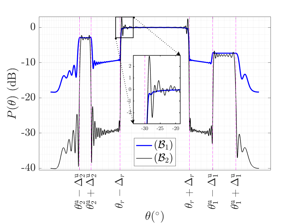
Figure 2: The resulting normalized beampatterns of $(\mathcal{B}_{1})$ and $(\mathcal{B}_{2})$. The radar operation is centered at $\theta_{r}=0^{\circ}$ with $\Delta_{r}=30^{\circ}$. The communication users are located at $\theta_{1}^{\tt{u}}=60^{\circ}$ and $\theta_{2}^{\tt{u}}=-60^{\circ}$. The problems were configured to beam-widths of $\Delta_{1}^{\tt{u}}=10^{\circ}$ and $\Delta_{2}^{\tt{u}}=5^{\circ}$. The power allocated for radar operation is $\varphi_{r}=0\operatorname{dB}$. The power allocated for users $1$ and $2$ correspond to $\varphi_{1}=-3\operatorname{dB}$ and $\varphi_{2}=-7.5\operatorname{dB}$, respectively.

VII Discussion

The reflected signal typically experiences a significant decrease in power due to double path-loss, consequently restricting detection performance unless dealt with pragmatically in practice. An area of active research involves integrating an analog-to-digital converter (ADC) model, such as $1$-bit or few-bit, that maps the analog signal, i.e. equation (11), to digital, i.e. (12) via an ADC function $\mathcal{Q}(.)$; see [33] and [34] for more details. Future investigations will delve into the estimation and detection limits with quantized received signals in order to examine the limitations of HRF when the reflected powers are significantly smaller than the direct LoS. Regardless of the scenario, the development of advanced algorithms specialized for low-resolution ADCs is essential to resolve these paths (see [35] for a proof-of-concept with $1-$bit ADC). Besides reflection powers versus user powers, future work will also accommodate power control mechanisms tailored for HRF as strong users should not overwhelm weaker users, which is of good advantage for low-resolution ADC structures [36]. As will be shown in the simulations section, the HRF has the potential of improving MSE performance on AoA, and in particular over mono-static communication-centric ISAC, as well as bi-static. This has a desirable impact not only on target sensing, but also on providing better channel estimates, which can be re-used for communication purposes. However, since we provide only a partial view of UL channels (i.e. delay, Doppler and gain are treated as nuisance parameters), then additional estimators are needed to compute the required sensing parameters. Hence, an overall improvement in MSE quality of sensing parameters has a direct impact on providing a better channel estimate, which has favorable returns on the decoding process for communications.

VIII Simulation Results

VIII-A Parameter Setup

Assume that both the transmit and receive antenna arrays are equipped with $N$ antennas and follow a uniform linear antenna (ULA) configuration spaced at half a wavelength, i.e. $\frac{\lambda}{2}$. The carrier frequency is set at $f_{c}=24$GHz. For OFDM transmissions, the subcarrier spacing is set to $\Delta_{f}=240$kHz; hence, the symbol duration is $T=\frac{1}{\Delta_{f}}=4.1667\mu$sec. The cyclic prefix duration is set to $T_{\text{CP}}=\frac{T}{4}=1.0417\mu$sec. Therefore, the total symbol duration is equal to $T_{o}=T+T_{\text{CP}}=5.2084\mu$sec. The constellation used is a quadrature phase shift keying (QPSK). Users are assumed to be located at equidistant angles, namely, the $k^{th}$ user is located at $\theta_{k}^{\tt{u}}=[-10-(k-1)\frac{60}{K-1}]^{\circ}$. All users are considered to be in LoS with the DFRC BS. Monte Carlo type experiments are conducted herein, where each trial generates an independent channel realization. The number of Monte Carlo simulations is set to $10^{4}$ trials. The MSE is computed as $\operatorname{MSE}=\frac{1}{qE}\sum_{e=1}^{E}\sum_{p=1}^{q}\big{(}\widehat{\theta}_{p}^{\tt{tar}}(e)-\theta_{k}\big{)}^{2}$, where $\widehat{\theta}_{p}^{\tt{tar}}(e)$ is the estimate of the $p^{th}$ target in the $e^{th}$ Monte Carlo experiment, and $E$ is the total number of experiments. All other parameters are mentioned in Section VIII-D.

The system setting adopted sets $d_{k}^{\tt{u}}=100$m for all users. The distances between the $k^{th}$ user and the $i^{th}$ target, i.e. $d_{k,i}$, are chosen from the $(k,i)^{th}$ entry of the following matrix

$$\boldsymbol{D}=\begin{bmatrix}64.8489&77.7906&94.2109\\ 68.6911&84.9746&100.8081\\ 74.9821&92.8385&107.1580\\ 82.8447&100.8129&112.9554\end{bmatrix}m.$$ (78)

On the other hand, the distance between the $i^{th}$ target and the DFRC BS, i.e. $d_{i}^{\tt{tar}}$ is selected from the $i^{th}$ entry of $i^{th}$ element of the following vector $\boldsymbol{d}^{\tt{tar}}=\begin{bmatrix}36&32.7951&27.0933\end{bmatrix}m$. Simulations consider either $1$ or $3$ targets. When $1$ target is selected, the index $i=1$ is used. The same approach is considered for users. The receive power is selected in a way to match the signal-to-noise ratio (SNR) for MSE evaluation.

VIII-B Benchmark Schemes

For the sake of performance comparisons, we include the following benchmarks in our performance study:

Naive MUSIC

We coin the term ”Naive MUSIC”, as the method which simply averages all the covariance matrices at hand to form a single covariance matrix $\widehat{\boldsymbol{R}}=\frac{1}{K}\sum_{k=1}^{K}\widehat{\boldsymbol{R}}_{k}$. This step is followed by an EVD to extract the signal and noise subspaces in order to compute the MUSIC criterion.

Algorithm 1 with prior knowledge of user AoAs

This benchmark runs Algorithm 1 under the condition that the true user AoAs are fed to the algorithm. More specifically, the first phase of Algorithm 1 is then unnecessary, and is therefore bypassed, because $\widehat{\theta}_{k}^{\tt{u}}$ are replaced by ${\theta}_{k}^{\tt{u}}$, for all $k=1\ldots K$. In practice, prior information can be leveraged with the aid of global navigation satellite system (GNSS) [37]. In [38], the authors used high-precision accuracy of $1$m. Note that centimeter and millimeter level accuracy is also possible [39]. An alternative is to run Algorithm 1 or Algorithm 2 without prior knowledge of user positions in a first stage, then utilize the estimated user positions in the second stage.

CRB

The CRB is a benchmark giving the lower bound on the variance of any unbiased estimator of deterministic parameters. Following the model introduced in Section II, the CRB of the target AoAs [40] can be shown to be

$$\operatorname{CRB}(\boldsymbol{\Theta}^{\tt{tar}})=\frac{\sigma^{2}}{2}\Big{(}\sum\nolimits_{k=0}^{K}\sum\nolimits_{\ell=0}^{\bar{L}_{k}}\boldsymbol{S}_{k}\boldsymbol{F}_{k,\ell}\boldsymbol{S}_{k}^{T}\Big{)}^{-1},$$ (79)

where

$$\boldsymbol{F}_{k,\ell}=\operatorname{Re}\{\operatorname{diag}(\boldsymbol{X}_{k}(:,\ell))^{*}\boldsymbol{H}_{k}\operatorname{diag}(\boldsymbol{X}_{k}(:,\ell))\},$$ (80)

$$\boldsymbol{H}_{k}=\boldsymbol{D}_{k}^{H}(\boldsymbol{I}-\boldsymbol{P}_{k})\boldsymbol{D}_{k}.$$ (81)

The expression of $\boldsymbol{P}_{k}$ is given in (31), $\boldsymbol{D}_{k}$ is the derivative of the manifold matrix given in (23), and $\boldsymbol{S}_{k}$ is a selection matrix indexing columns of the common manifold matrix, $\boldsymbol{A}({\boldsymbol{\Theta}}^{\tt{tar}})$. Also, the CRB of the monostatic and bistatic cases (for $K=1$) are also illustrated to show the advantage of the hybrid scheme. The communication-centric mono-static ISAC CRB accounts only for the DL, hence it contains only the $k=0$ term. The communication-centric bi-static ISAC CRB, on the other hand, incorporates the UL terms, i.e. the $k=1\ldots K$ terms.

VIII-C Scenarios

We distinguish between two scenarios:

• Scenario $1$: Here, the product of the number of subcarriers and the number of OFDM symbols are set to be equal. In other words, for any $K$ users, the factor $L_{k}|\mathcal{C}_{k}|$ is held constant for all $k$. The aim of studying this scheme is to show the performance of time-frequency resource fairness and its impact on the MSE of the estimated AoAs via the different methods described in this article. Specifically, if $K$ users are participating in the UL, the $k^{th}$ user is allocated $|\mathcal{C}_{k}|=\frac{32}{K}$ subcarriers, and $L_{k}=16K$ symbols.

• Scenario $2$: In this scenario, we fix the number of OFDM symbols to $L_{k}=32$ for each users and allocate $|\mathcal{C}_{k}|=32$ subcarriers for each user. In other words, more users participating in the UL requires more bandwidth.

VIII-D Simulation Results

(a) $N=5$ antennas

(b) $N=10$ antennas

Figure 3: Scenario 1: The MSE versus SNR of the proposed methods and benchmarks for different number of users and $q=1$ target located at $0^{\circ}$.

Scenario $1$ with a single target

In Fig. 3, we plot the MSE of the estimated AoAs as a function of varying SNR, for different number of antennas. In Fig. 3a, we fix $N=5$ antennas and $q=1$ target located at $\theta_{1}^{\tt{tar}}=0^{\circ}$. We see that Algorithm 1 with AoA prior achieves the best performance for any $K$ as compared to other methods, which is caused by less unknown parameters being estimated than other presented methods. Interestingly, as $K$ increases, Algorithm 1 without the user AoA prior knowledge coincides with that with prior information. Moreover, both versions of Algorithm 1 achieve the CRB starting at an SNR of $2\operatorname{dB}$. On the other hand, for an MSE accuracy of $10^{-4}$, Algorithm 2 loses about $4\operatorname{dB}$ in SNR as compared to Algorithm 1, and outperforms the Naive MUSIC benchmark, even at high SNR. When more users are participating in the UL, we see that doubling the number of users contributes to an overall MSE improvement of about $3.2\operatorname{dB}$. This can be explained through time diversity, i.e. the participation of more users within the same bandwidth, but through the availability of more OFDM symbols. In Fig. 3b, we fix $N=10$ antennas, as well as $q=1$ target with $\theta_{1}^{\tt{tar}}=0^{\circ}$. We can notice that both versions of Algorithm 1 achieve the CRB for all $K$, with an improved performance over that in Fig. 3a due to an increase in number of antennas. Moreover, as more users participate in the UL, the performance of both versions of Algorithm 1 approaches its CRB faster. This is due to the participation of more users in the UL over the same bandwidth resource. For instance, at $\operatorname{SNR}=-20\operatorname{dB}$, Algorithm 1 is only $0.0017\operatorname{rad}^{2}$ far away from its CRB for $K=4$, and $0.18\operatorname{rad}^{2}$ for $K=1$. Moreover, we see that for increasing $K$, Algorithm 1 approaches the version of itself with prior user AoAs, which is explained through time diversity, i.e. when more OFDM symbols are available at the disposal of the DFRC BS, a better MSE performance is expected, in general. In particular, for an accuracy of $10^{-3}$, and for $K=1$, the gap between both versions of Algorithm 1 is $1.2\operatorname{dB}$, compared to $1\operatorname{dB}$ for $K=2$, and $0.7\operatorname{dB}$ for $K=4$. Algorithm 2 generally performs better than the Naive MUSIC benchmark in the high SNR regime. For example, at $K=2$, the performance of Algorithm 2 begins to outperform the Naive MUSIC benchmark starting from $\operatorname{SNR}=-11\operatorname{dB}$, and $\operatorname{SNR}=-7\operatorname{dB}$ for $K=8$, which can also be explained through more users transmitting in the UL, thus providing more OFDM samples towards the DFRC BS. We notice that for both $N=5$ and $N=10$ cases, the CRB of the mono-static and bi-static are very close. In fact, the HRF CRB for only $K=1$ user, improves the MSE by nearly $5\operatorname{dB}$.

(a) $N=5$ antennas

(b) $N=10$ antennas

Figure 4: Scenario 1: The MSE versus SNR of the proposed methods and benchmarks for a different number of users and $q=3$ targets located at $0^{\circ},30^{\circ},60^{\circ}$.

Scenario $1$ with multiple targets

In Fig. 4, we follow the same scenario as in Fig. 3, but this time tripling the number of targets, i.e. $q=3$. The targets are assumed to be located at $0^{\circ},30^{\circ},60^{\circ}$, respectively. This study will show the improvements of MSE estimates with an increasing number of users, even with more targets. The number of subcarriers and OFDM symbols for the $k^{th}$ user is also the same as that in Fig. 3. Note that the case of $K=0$ refers to the mono-static only case, where only the echo received due to the DL signal is used at the DFRC BS. In Fig. 4a, we fix $N=5$ antennas. As was previously the case, we can observe that the benchmark of Algorithm 1 with AoA prior achieves the best performance for a different number of users. The improvement of performance with increasing users is still preserved, as we see a factor of $3\operatorname{dB}$ gain in CRB, when doubling $K$. Nevertheless, both versions of Algorithm 1 achieve the CRB starting at $\operatorname{SNR}=0\operatorname{dB}$. Moreover, we see that Algorithm 2 generally outperforms the Naive MUSIC benchmark starting from $\operatorname{SNR}=-11\operatorname{dB}$ for $K=1$, $\operatorname{SNR}=-10\operatorname{dB}$ for $K=8$, which can also be explained by the availability of more time resources, which becomes more notable for a higher number of users. In Fig. 4b, we fix $N=10$ antennas, as well as $q=3$ targets. We can also say that the gap between both versions of Algorithm 1 shrinks with increasing $K$. For e.g., both versions coincide at an accuracy of $10^{-2}$ and for $K=16$, as compared to a $0.5\operatorname{dB}$ gap for $K=1$. The Naive MUSIC benchmark also approaches the CRB for higher $N$, but saturates after $\operatorname{SNR}=4\operatorname{dB}$ for $K=1,2$. This loss of performance in Naive MUSIC is due to the fact that it does not exploit the common manifold and, so, treats all AoAs, whether targets or users, equally. We observe that for $N=5$ antennas the CRB for the single-user (SU) HRF improves that of the mono-static by $5\operatorname{dB}$, whereas there is a $10\operatorname{dB}$ gap between the mono-static and bi-static cases. For $N=10$, we see that the bi-static CRB approaches that of the mono-static. However, the SU HRF improves by $4\operatorname{dB}$.

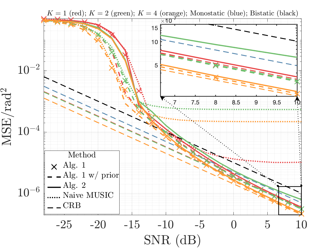
(a) $N=5$ antennas

(b) $N=10$ antennas

Figure 5: Scenario 2: The MSE versus SNR of the proposed methods and benchmarks for different number of users and $q=1$ target located at $0^{\circ}$.

Scenario $2$ with a single target

In Fig. 5, we switch to Scenario $2$, where we plot the MSE of the estimated AoAs as a function of varying SNR, for different number of antennas. As done previously, we study the performance for $N=5$ and $N=10$ antennas. In Fig. 5a, we fix $N=5$ antennas for a single target located at $0^{\circ}$. As is the case in previous experiments, both versions of Algorithm 1 coincide and meet the CRB at high SNR. Also, Algorithm 2 decays with the CRB, however, the MSE of Naive MUSIC saturates with increasing SNR. For instance, focusing on $K=2$, we can see that at $\operatorname{SNR}=-14\operatorname{dB}$, the MSE curve of Naive MUSIC begins to saturate, whereas the MSE of Algorithm 2 approaches the CRB with an increase of SNR. This is explained through Algorithm 2’s effectiveness in segregating the common manifold. A similar observation is given for all other values of $K$. In Fig. 5b, we fix $N=10$ antennas with a single source as in Fig. 5a. We can also report that both versions of Algorithm 1 converge towards the CRB at high SNR. Furthermore, for an MSE level of $10^{-4}\operatorname{rad}^{2}$, there is a $0.4\operatorname{dB}$ gain when doubling the number of users from $K=1$ to $K=2$, followed by a gain of $0.6\operatorname{dB}$ between $K=2$ and $K=4$. This gain is explained via the availability of more bandwidth, where by increasing $K$, we also increase the bandwidth to accommodate users. Moreover, each user will provide a better spatial view of the target through its UL contribution. We notice that the CRB for the $K=1$ case of HRF improves the mono-static CRB by $1.8\operatorname{dB}$, and $4.8\operatorname{dB}$ better than the bi-static configuration.

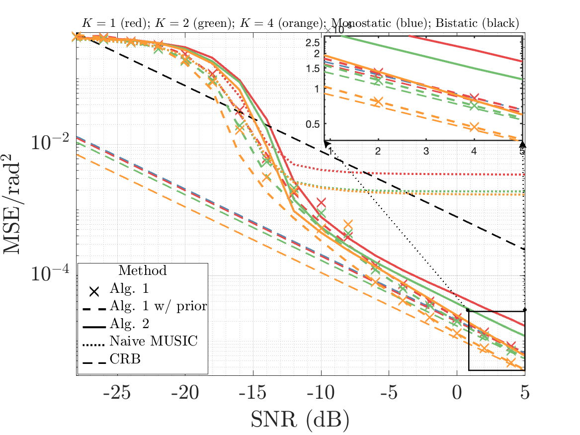
(a) $N=5$ antennas

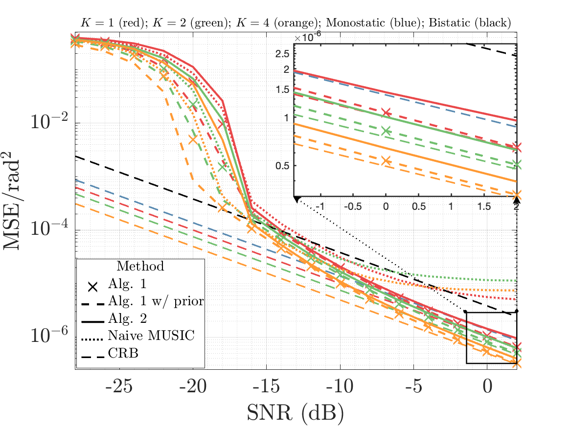
(b) $N=10$ antennas

Figure 6: Scenario 2: The MSE versus SNR of the proposed methods and benchmarks for a different number of users and $q=3$ targets located at $0^{\circ},30^{\circ},60^{\circ}$.

Scenario $2$ with multiple targets

In Fig. 6, we follow the same scenario as that in Fig. 5, but we place $q=3$ targets, instead of $q=1$. As is the case in Fig. 4, the targets are assumed to be located at $0^{\circ},30^{\circ},60^{\circ}$, respectively. We aim to study the performance with multiple targets. In Fig. 6a, we fix $N=5$ and $q=3$. We observe that both versions of Algorithm 1 coincide with the CRB as SNR increases. Observe that, in general, Naive MUSIC saturates earlier than the case of $q=1$, i.e. compared to Fig. 5a. For e.g., at $K=1$, the Naive MUSIC begins to saturate at $\operatorname{SNR}=-10\operatorname{dB}$ at an MSE level of about $0.003\operatorname{rad}^{2}$, as compared to $10^{-5}\operatorname{rad}^{2}$ at $\operatorname{SNR}=0\operatorname{dB}$, in Fig. 5a. This goes ahead to show that Naive MUSIC is expected to do worse for more targets, due to its inability to distinguish the common target manifold. In contrast, Algorithm 2 approaches the CRB for high SNR. In Fig. 6b, we fix $N=10$ and $q=3$. Again, we observe that both versions of Algorithm 1 converge to the CRB at high SNR, whereas the Naive MUSIC saturates. Algorithm 2 decays with the CRB for high SNR. We also see gains for Algorithm 2, when compared to Naive MUSIC. For e.g., at an MSE level of $10^{-5}\operatorname{rad}^{2}$ and at $K=1$, we see that Algorithm 2 gains about $2.5\operatorname{dB}$ compared to Naive MUSIC and a $5\operatorname{dB}$ gain for $K=4$. Moreover, by referring to Fig. 6b, we notice that the SU HRF CRB is $1.3\operatorname{dB}$ better than the mono-static case, and also improves the bi-static case by $5\operatorname{dB}$.

Figure 7: Behavior of the different algorithms as a function of iteration number.

AoA Behavior

In Fig. 7, we study the estimated AoA behavior of the proposed methods as a function of iteration number. The estimate of each AoA at any given iteration is averaged over Monte Carlo trials. The chosen $\operatorname{SNR}$ is $-12\operatorname{dB}$, $N=5$ and $K=16$. We observe that all methods converge, even at low $\operatorname{SNR}$. Even more, when the user AoAs are fed as prior information into Algorithm 1, we can see a slightly faster convergence than the case without prior information, most notably around the $3^{rd}$ iteration in an attempt to estimate $\theta_{3}^{\tt{tar}}=60^{\circ}$. Also, all methods converge after $5$ iterations. This proves the effectiveness and stability of the proposed methods, from a convergence viewpoint, even at low $\operatorname{SNR}$.

Figure 8: A spectrum comparison of $h^{-1}(\theta)$ given in Algorithm 2 vs. the MUSIC spectrum. Vertical dashed lines correspond to the true target AoAs.

Spectra Comparison

In Fig. 8, we reveal some internal dynamics of Algorithm 2, namely the spectrum $h^{-1}(\theta)$, where its maximization is involved within the second phase of Algorithm 2. So, a reasonable comparison of spectra would be $h^{-1}(\theta)$, compared to the classical MUSIC spectrum. Besides, the spectra of each method have been averaged over multiple trials. Herein, we fix $\operatorname{SNR}=10\operatorname{dB}$, $K=16$ users, $q=3$ located at $0^{\circ},30^{\circ},60^{\circ}$ and $N=5$. Not only can we notice an accurate estimation of the true target AoAs, but we can also report sharper peaks and an improved resolution, as compared to the Naive MUSIC one, which further allows for better target AoA estimation. Also, notice that the noise level of the spectra has been reduced by more than $6\operatorname{dB}$, especially around the region $[-70^{\circ},-50^{\circ}]$. This again proves the superiority of Algorithm 2, when compared to MUSIC.

Figure 9: The different spectra, i.e. $g_{1}^{-1}(\theta)\ldots g_{K}^{-1}(\theta)$, involved in the first phase of Algorithm 2. Vertical dashed lines correspond to the true user AoAs.

Behavior of $g(\theta)$

In Fig. 9, we further highlight additional dynamics of Algorithm 2, namely the spectrum $g_{k}^{-1}(\theta)$, found in the first phase of Algorithm 2. As a reminder, the $k^{th}$ spectrum, $g_{k}^{-1}(\theta)$, aids in identifying the AoA of the $k^{th}$ user. As is the case of Fig. 8, each spectrum is averaged over different Monte Carlo trials. The $\operatorname{SNR}$ is set to $10\operatorname{dB}$, the number of users is set to $K=16$, and the number of antennas is set to $N=5$ antennas. First, we can see one and only one peak for any $g_{k}^{-1}(\theta)$. This is a good indicator, as $g_{k}^{-1}(\theta)$ should be highly selective of its associated user (i.e. the $k^{th}$ user) and also capable of simultaneously rejecting off all other users and targets, even with a low number of antennas i.e., $N=5$. With this feature in mind, we see that there are no spurious peaks arising in any of the spectra. Moreover, we can observe that the peaks sharpen, as the user approaches the broad-fire of the antenna array. Furthermore, we notice that the noise levels decrease as the user approaches the end-fire of the antenna array, which is a typical characteristic of ULA.

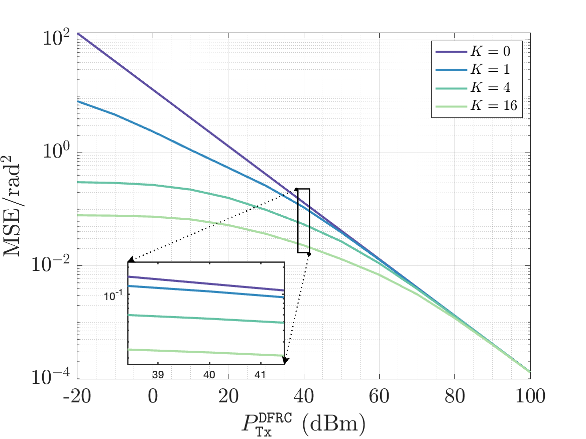
Figure 10: The CRB performance as a function of transmit DFRC BS power for a typical mmWave communication system.

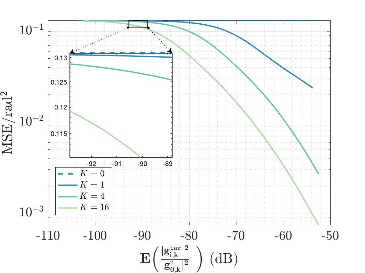
Figure 11: The CRB performance as a function of mean reflection-to-LoS power for a typical mmWave communication system at $P_{\tt{Tx}}^{\tt{DFRC}}=40\operatorname{dBm}$.

HRF Necessity

In practical scenarios, the communication user is characterized by a notably lower transmission power and deploys a comparatively smaller antenna array in contrast to the infrastructure of the DFRC BS [41]. The purpose of the simulation depicted in Fig. 10 is to examine the conditions where the utilization of the HRF becomes imperative for enhancing sensing performance across a range of diverse communication users. For that, we have utilized the same simulation parameters as those for a typical mmWave communication system [41] (c.f. Table XIV), and we have set the total power transmitted by the DFRC BS as $P_{\tt{Tx}}^{\tt{DFRC}}$ to study the attainable CRB for various number of UL users. We notice that at $P_{\tt{Tx}}^{\tt{DFRC}}=40\operatorname{dBm}$, which is the transmit power of a BS in typical mmWave systems [41], the HRF continues to bestow tangible sensing advantages with increasing number of users. For example, when $K=0$ the CRB is $0.13\operatorname{rad}^{2}$ and with the advent of $K=1$, the CRB experiences a reduction to $0.1\operatorname{rad}^{2}$. Upon quadrupling the user count, a proportionate reduction factor of $2$ emerges, resulting in CRB values of $0.05\operatorname{rad}^{2}$ for $K=4$ and $0.025\operatorname{rad}^{2}$ for $K=16$. Another noteworthy aspect to consider is the threshold transmit power level at which the HRF may no longer be useful. At $52\operatorname{dBm}$, it becomes evident that the performance of a single user ($K=1$) in the HRF scheme aligns closely with the performance of the DFRC BS operating in isolation. Similarly, when the transmit power exceeds $66\operatorname{dBm}$, we observe that the performance of the HRF scheme with $K=4$ coincides with that of the DFRC BS only-case. Moreover, upon reaching a transmit power of $78\operatorname{dBm}$, the convergence persists, with $K=16$ users in the HRF scheme closely mirroring the performance of the DFRC BS in standalone operation. The insight derived from these observations suggests that, in scenarios where transmit power surpasses the specified thresholds, the deployment of the HRF scheme may not yield substantial additional sensing gains beyond the capabilities of the DFRC operating independently. In Fig. 11, we aim to study the CRB evolution as a function of the ratio of the reflected power to the direct LoS transmission power. In this simulation, we fix $P_{\tt{Tx}}^{\tt{DFRC}}=40\operatorname{dBm}$ as specified in [41]. In the general case, our simulations reveal that the advantages of HRF remain significant, particularly when reflection-to-LoS power ratio is reasonable, and for increasing $K$. When the ratio between reflection-to-LoS power ratio falls below the threshold of $-90\operatorname{dB}$, the performance for $K=1$ users aligns with that of the standalone DFRC BS. Similarly, as the reflection-to-LoS power ratio decreases to values below $-96\operatorname{dB}$ and $-102\operatorname{dB}$, the performance for $K=4$ and $K=16$ users respectively coincides with that of the DFRC BS operating on its own. The observations suggest that as the reflection-to-LoS ratio decreases below certain thresholds, the performance of multiple users contributing to HRF approaches the performance level exhibited by the standalone DFRC BS. In addition, these thresholds decrease with increasing number of users participating for HRF operations. This insight underscores the significance of the reflection-to-LoS ratio in determining the system’s capability to support multiple users and indicates a critical threshold where the system’s performance is notably affected by the ratio of reflected to direct signals. In general, we see that quadrupling the number of users requires $6\operatorname{dB}$ to $7\operatorname{dB}$ less reflection power to achieve the same CRB performance.

IX Conclusions and Outlook

In this paper, a new hybrid radar model is proposed, where the DFRC BS acts as a monostatic radar in the DL and users act as distributed bistatic radars in the UL, following an FDD protocol. From the DFRC perspective, we derive the ML criterion of the AoA estimation problem, and assemble its connections with the classical AoA estimation problem. We take a step further in proposing two efficient estimators. The first one is built on the direct optimization of the FML criterion by alternating between user and target terms in the ML cost function. Furthermore, the second method diligently forms an iterative procedure via the formulation of suitable optimization methods that exploit the common manifold structure appearing over different communication bands. Our simulation findings prove the effectiveness of the proposed hybrid radar model, along with methods involved in resolving and estimating the locations. In short, the proposed communication-centric hybrid radar model has proven its potential and superiority in improving target location estimates in different settings.

Research directions include extensions toward wide-band, which further lead to frequency-dependent array response vectors. Also, due to full duplex operation, we plan to propose estimators, and compensators, for the self-interference leakage phenomenon caused by the transmitting onto the receipting unit of the DFRC BS. Another direction is the multi-parameter estimation case, where the ToA and Doppler parameters are to be jointly estimated with AoAs. Moreover, from an estimation perspective, we also allude to the need for more sophisticated algorithms that trade complexity for performance.

References

- [1] J. A. Zhang, M. L. Rahman, K. Wu, X. Huang, Y. J. Guo, S. Chen, and J. Yuan, “Enabling Joint Communication and Radar Sensing in Mobile Networks—A Survey,” IEEE Communications Surveys & Tutorials, vol. 24, no. 1, pp. 306–345, 2022.
- [2] F. Liu, C. Masouros, A. P. Petropulu, H. Griffiths, and L. Hanzo, “Joint Radar and Communication Design: Applications, State-of-the-Art, and the Road Ahead,” IEEE Transactions on Communications, vol. 68, no. 6, pp. 3834–3862, 2020.
- [3] K. V. Mishra, M. Bhavani Shankar, V. Koivunen, B. Ottersten, and S. A. Vorobyov, “Toward Millimeter-Wave Joint Radar Communications: A Signal Processing Perspective,” IEEE Signal Processing Magazine, vol. 36, no. 5, pp. 100–114, 2019.
- [4] A. Liu, Z. Huang, M. Li, Y. Wan, W. Li, T. X. Han, C. Liu, R. Du, D. K. P. Tan, J. Lu, Y. Shen, F. Colone, and K. Chetty, “A Survey on Fundamental Limits of Integrated Sensing and Communication,” IEEE Communications Surveys & Tutorials, vol. 24, no. 2, pp. 994–1034, 2022.
- [5] M. Chafii, L. Bariah, S. Muhaidat, and M. Debbah, “Twelve Scientific Challenges for 6G: Rethinking the Foundations of Communications Theory,” IEEE Communications Surveys & Tutorials, pp. 1–1, 2023.
- [6] J. Choi, V. Va, N. Gonzalez-Prelcic, R. Daniels, C. R. Bhat, and R. W. Heath, “Millimeter-Wave Vehicular Communication to Support Massive Automotive Sensing,” IEEE Communications Magazine, vol. 54, no. 12, pp. 160–167, 2016.
- [7] X. Cheng, D. Duan, S. Gao, and L. Yang, “Integrated Sensing and Communications (ISAC) for Vehicular Communication Networks (VCN),” IEEE Internet of Things Journal, vol. 9, no. 23, pp. 23 441–23 451, 2022.
- [8] H. Zhang, H. Zhang, B. Di, M. D. Renzo, Z. Han, H. V. Poor, and L. Song, “Holographic Integrated Sensing and Communication,” IEEE Journal on Selected Areas in Communications, vol. 40, no. 7, pp. 2114–2130, 2022.
- [9] F. Liu, Y. Cui, C. Masouros, J. Xu, T. X. Han, Y. C. Eldar, and S. Buzzi, “Integrated sensing and communications: Toward dual-functional wireless networks for 6g and beyond,” IEEE Journal on Selected Areas in Communications, vol. 40, no. 6, pp. 1728–1767, 2022.
- [10] Z. Xiao and Y. Zeng, “Waveform Design and Performance Analysis for Full-Duplex Integrated Sensing and Communication,” IEEE Journal on Selected Areas in Communications, vol. 40, no. 6, pp. 1823–1837, 2022.
- [11] J. Mu, R. Zhang, Y. Cui, N. Gao, and X. Jing, “UAV Meets Integrated Sensing and Communication: Challenges and Future Directions,” IEEE Communications Magazine, pp. 1–7, 2022.
- [12] A. Bazzi and M. Chafii, “On Outage-based Beamforming Design for Dual-Functional Radar-Communication 6G Systems,” IEEE Transactions on Wireless Communications, pp. 1–1, 2023.
- [13] Q. Qi, X. Chen, C. Zhong, and Z. Zhang, “Integrated Sensing, Computation and Communication in B5G Cellular Internet of Things,” IEEE Transactions on Wireless Communications, vol. 20, no. 1, pp. 332–344, 2021.
- [14] J. A. Zhang, F. Liu, C. Masouros, R. W. Heath, Z. Feng, L. Zheng, and A. Petropulu, “An Overview of Signal Processing Techniques for Joint Communication and Radar Sensing,” IEEE Journal of Selected Topics in Signal Processing, vol. 15, no. 6, pp. 1295–1315, 2021.
- [15] R. M. Mealey, “A Method for Calculating Error Probabilities in a Radar Communication System,” IEEE Transactions on Space Electronics and Telemetry, vol. 9, no. 2, pp. 37–42, 1963.
- [16] A. Bazzi and M. Chafii, “On Integrated Sensing and Communication Waveforms with Tunable PAPR,” IEEE Transactions on Wireless Communications, pp. 1–1, 2023.
- [17] A. Hassanien, M. G. Amin, Y. D. Zhang, and F. Ahmad, “Dual-Function Radar-Communications: Information Embedding Using Sidelobe Control and Waveform Diversity,” IEEE Transactions on Signal Processing, vol. 64, no. 8, pp. 2168–2181, 2016.
- [18] T. Huang, N. Shlezinger, X. Xu, Y. Liu, and Y. C. Eldar, “MAJoRCom: A Dual-Function Radar Communication System Using Index Modulation,” IEEE Transactions on Signal Processing, vol. 68, pp. 3423–3438, 2020.
- [19] A. Hassanien, M. G. Amin, Y. D. Zhang, and F. Ahmad, “Signaling strategies for dual-function radar communications: an overview,” IEEE Aerospace and Electronic Systems Magazine, vol. 31, no. 10, pp. 36–45, 2016.
- [20] A. Hassanien, M. G. Amin, E. Aboutanios, and B. Himed, “Dual-Function Radar Communication Systems: A Solution to the Spectrum Congestion Problem,” IEEE Signal Processing Magazine, vol. 36, no. 5, pp. 115–126, 2019.
- [21] S. D. Liyanaarachchi, T. Riihonen, C. B. Barneto, and M. Valkama, “Optimized Waveforms for 5G–6G Communication With Sensing: Theory, Simulations and Experiments,” IEEE Transactions on Wireless Communications, vol. 20, no. 12, pp. 8301–8315, 2021.
- [22] L. Leyva, D. Castanheira, A. Silva, and A. Gameiro, “Two-stage estimation algorithm based on interleaved OFDM for a cooperative bistatic ISAC scenario,” in 2022 IEEE 95th Vehicular Technology Conference: (VTC2022-Spring), 2022, pp. 1–6.
- [23] Z. Yu, X. Hu, C. Liu, M. Peng, and C. Zhong, “Location Sensing and Beamforming Design for IRS-Enabled Multi-User ISAC Systems,” IEEE Transactions on Signal Processing, vol. 70, pp. 5178–5193, 2022.
- [24] L. Pucci, E. Paolini, and A. Giorgetti, “System-Level Analysis of Joint Sensing and Communication Based on 5G New Radio,” IEEE Journal on Selected Areas in Communications, vol. 40, no. 7, pp. 2043–2055, 2022.
- [25] F. Liu, L. Zhou, C. Masouros, A. Li, W. Luo, and A. Petropulu, “Toward Dual-functional Radar-Communication Systems: Optimal Waveform Design,” IEEE Transactions on Signal Processing, vol. 66, no. 16, pp. 4264–4279, 2018.
- [26] N. Su, F. Liu, and C. Masouros, “Sensing-Assisted Eavesdropper Estimation: An ISAC Breakthrough in Physical Layer Security,” arXiv preprint arXiv:2210.08286, 2022.
- [27] Z. Huang, K. Wang, A. Liu, Y. Cai, R. Du, and T. X. Han, “Joint Pilot Optimization, Target Detection and Channel Estimation for Integrated Sensing and Communication Systems,” IEEE Transactions on Wireless Communications, vol. 21, no. 12, pp. 10 351–10 365, 2022.
- [28] Z. Gao, Z. Wan, D. Zheng, S. Tan, C. Masouros, D. W. K. Ng, and S. Chen, “Integrated Sensing and Communication With mmWave Massive MIMO: A Compressed Sampling Perspective,” IEEE Transactions on Wireless Communications, vol. 22, no. 3, pp. 1745–1762, 2023.
- [29] C. R. Rao, H. Toutenburg, H. C. Shalabh, and M. Schomaker, “Linear models and generalizations,” Least Squares and Alternatives (3rd edition) Springer, Berlin Heidelberg New York, 2008.
- [30] I. Ziskind and M. Wax, “Maximum likelihood localization of multiple sources by alternating projection,” IEEE Transactions on Acoustics, Speech, and Signal Processing, vol. 36, no. 10, pp. 1553–1560, 1988.
- [31] A. Bazzi and D. Slock, “Robust Music Estimation Under Array Response Uncertainty,” in ICASSP 2020 - 2020 IEEE International Conference on Acoustics, Speech and Signal Processing (ICASSP), 2020, pp. 4821–4825.
- [32] K. B. Petersen, M. S. Pedersen et al., “The matrix cookbook,” Technical University of Denmark, vol. 7, no. 15, p. 510, 2008.
- [33] J. Mo, P. Schniter, and R. W. Heath, “Channel Estimation in Broadband Millimeter Wave MIMO Systems With Few-Bit ADCs,” IEEE Transactions on Signal Processing, vol. 66, no. 5, pp. 1141–1154, 2018.
- [34] A. Mezghani and A. L. Swindlehurst, “Blind Estimation of Sparse Broadband Massive MIMO Channels with Ideal and One-bit ADCs,” IEEE Transactions on Signal Processing, vol. 66, no. 11, pp. 2972–2983, 2018.
- [35] P. Kumari, A. Mezghani, and R. W. Heath, “A Low-Resolution ADC Proof-of-Concept Development for a Fully-Digital Millimeter-wave Joint Communication-Radar,” in ICASSP 2020 - 2020 IEEE International Conference on Acoustics, Speech and Signal Processing (ICASSP), 2020, pp. 8619–8623.
- [36] S. Jacobsson, G. Durisi, M. Coldrey, U. Gustavsson, and C. Studer, “Throughput Analysis of Massive MIMO Uplink With Low-Resolution ADCs,” IEEE Transactions on Wireless Communications, vol. 16, no. 6, pp. 4038–4051, 2017.
- [37] A. Kakkavas, G. Seco-Granados, H. Wymeersch, M. H. C. Garcia, R. A. Stirling-Gallacher, and J. A. Nossek, “5G Downlink Multi-Beam Signal Design for LOS Positioning,” in 2019 IEEE Global Communications Conference (GLOBECOM), 2019, pp. 1–6.
- [38] N. Garcia, H. Wymeersch, E. G. Ström, and D. Slock, “Location-aided mm-wave channel estimation for vehicular communication,” in 2016 IEEE 17th International Workshop on Signal Processing Advances in Wireless Communications (SPAWC), 2016, pp. 1–5.
- [39] D. Odijk and P. J. G. Teunissen, High-Precision GNSS. Cham: Springer International Publishing, 2016, pp. 1–7. [Online]. Available: https://doi.org/10.1007/978-3-319-02370-0_8-1
- [40] P. Stoica and A. Nehorai, “MUSIC, maximum likelihood, and Cramer-Rao bound,” IEEE Transactions on Acoustics, Speech, and Signal Processing, vol. 37, no. 5, pp. 720–741, 1989.
- [41] I. A. Hemadeh, K. Satyanarayana, M. El-Hajjar, and L. Hanzo, “Millimeter-Wave Communications: Physical Channel Models, Design Considerations, Antenna Constructions, and Link-Budget,” IEEE Communications Surveys & Tutorials, vol. 20, no. 2, pp. 870–913, 2018.