Detection of a new molecular cloud in the LHAASO J2108+5157 region supporting a hadronic PeVatron scenario

Abstract

PeVatrons are the most powerful naturally occurring particle accelerators in the Universe. The identification of counterparts associated to astrophysical objects such as dying massive stars, molecular gas, star-forming regions, and star clusters is essential to clarify the underlying nature of the PeV emission, i.e., hadronic or leptonic. We present ^12,13CO(J=2$\rightarrow$1) observations made with the 1.85 m radio-telescope of the Osaka Prefecture University toward the Cygnus OB7 molecular cloud, which contains the PeVatron candidate LHAASO J2108+5157. We investigate the nature of the sub-PeV (gamma-ray) emission by studying the nucleon density determined from the content of HI and H₂, derived from the CO observations. In addition to MML[2017]4607, detected via the observations of the optically thick ¹²CO(J=1$\rightarrow$0) emission, we infer the presence of an optically thin molecular cloud, named [FKT-MC]2022, whose angular size is 1.1$\pm$0.2^∘. We propose this cloud as a new candidate to produce the sub-PeV emission observed in LHAASO J2108+5157. Considering a distance of 1.7 kpc, we estimate a nucleon (HI+H₂) density of 37$\pm$14 cm^-3, and a total nucleon mass(HI+H₂) of 1.5$\pm$0.6$\times$10⁴ M_⊙. On the other hand, we confirm that Kronberger 82 is a molecular clump with an angular size of 0.1^∘, a nucleon density $\sim$ 10³ cm^-3, and a mass $\sim$ 10³ M_⊙. Although Kronberger 82 hosts the physical conditions to produce the observed emission of LHAASO J2108+5157, [FKT-MC]2022 is located closer to it, suggesting that the latter could be the one associated to the sub-PeV emission. Under this scenario, our results favour a hadronic origin for the emission.

1 Introduction

While human-manufactured particle accelerators can achieve relatively high energies, up to 14 TeV (in a collision) with the Large Hadron Collider, and is planned to reach values as high as 100 TeV via the future circular collider in the 2040 decade, it is known that in the Universe there are natural sources that can accelerate particles reaching energies up to hundreds of Exa eV (EeV). Thus, one of the fundamental questions in high energy physics is: what is the maximum energy to which nature accelerates particles in the Galaxy?. The answer to this question can be obtained by studying high-energy radiation and astroparticles (cosmic-ray, neutrinos, and gamma-rays) produced by one type of the most powerful natural particle accelerators: PeVatrons. Although there is no consensus on its definition, a PeVatron can be considered an astronomical object that can accelerate particles up to PeV energies.

Since high-energy particles produce gamma rays and X-rays, they are studied within the field known as Gamma-Ray Astrophysics (GRA). This new research field provides key knowledge to our understanding of the physical laws and mechanisms underlying particle acceleration. In addition, given that cosmic particle accelerators are also sources of non-thermal radiation, GRA creates a connection between the study of high-energy cosmic rays, neutrinos, and gravitational waves and the multi-wavelength astronomy.

The energy regime of the emission studied in GRA can be divided in three: High Energy (0.1-100 GeV), Very High Energy (VHE) (0.1-100 TeV), and Ultra High Energy (UHE) (0.1-100 PeV). Since its emergence as a research field, GRA has gone through three eras sparked by major revolutions: 1.- The discovery of energetic phenomena in the Universe (e.g. the Galactic diffuse gamma rays and the gamma-ray pulsars; the GeV era) by satellite gamma-ray detectors (e.g. EGRET, FERMI-LAT), 2.- The development of water Cherenkov (e.g. Milagro and HAWC) and imaging air Cherenkov observatories; the construction of extensive (surface) air shower arrays (e.g. MAGIC, H.E.S.S., VERITAS, ARGO-YBJ, Tibet AS$\gamma$), which discovered extremely powerful objects like supernova remnants, pulsar wind nebulae, TeV Halos objects, binaries systems, and active galactic nuclei); the TeV era, and 3.- The rise of the UHE observations and the discovery of PeVatrons by HAWC, Tibet AS$\gamma$ and LHAASO observations: the PeV era.

While cosmic rays with energies $<$ 1 PeV are thought to have a Galactic origin, those with energies $>$ 1 EeV are thought to originate in extra-galactic sources. The transition in between is investigated through the study of PeVatrons. Since 2019, the Tibet AS$\gamma$ (Amenomori et al., 2019, 2021a, 2021b, 2021c), HAWC (Abeysekara et al., 2020, 2021; Albert et al., 2020a), and LHAASO (Cao et al., 2021a, b) experiments have detected a dozen of UHE sources on the Galactic plane. Thus, thanks to PeV astronomy, we became able to investigate particle acceleration within the Galaxy beyond the PeV energy regime. On the other hand, the question of whether only hadrons (protons) or leptons (electrons) should be considered in the acceleration process is critical to understand, e.g., the underlying nature of the observed gamma ray radiation.

To explain the production of the UHE gamma rays, two scenarios have been proposed: 1. Neutral pions decay caused by the interaction of PeV protons with molecular material of the ambient interstellar medium (ISM), known as the hadronic scenario, and 2. Inverse Compton (IC) scattering, caused by high-energy electrons scattering off ambient interstellar cosmic background photons, diffusive starlight and Galactic interstellar IR emission. This one is known as the leptonic scenario. The detection and characterization of atomic hydrogen (HI) and molecular gas are crucial to estimate the density of nucleons that could be interacting with high-energy cosmic rays. This would shed light on determining which of the two proposed gamma-ray emission mechanisms is playing a major role. The most used proxy to probe the physical properties of the neutral molecular component of the ISM is the CO molecule. To this end, CO emission lines are widely used to trace the cold (10–30 K), and dense (10³–10⁴ cm^-3) molecular gas phase of the ISM in the Galaxy (e.g Sano et al., 2020; Fukui et al., 2021). A detailed survey and study of CO emission from the ISM is necessary to characterize the physical conditions of molecular clouds and material lying nearby gamma-ray sources, which will allow to elucidate the nature and the origin of the high-energy cosmic rays. Therefore, without minimizing the co-acceleration (hadrons and leptons), carrying out a detailed study of the molecular gas in the vicinity of a PeVatron is essential to explore the hadronic nature of the gamma ray emission.

HAWC (Abeysekara et al., 2021; Albert et al., 2021), Tibet AS$\gamma$ (Amenomori et al., 2021c) and LHAASO (Cao et al., 2021a) have confirmed the presence of three PeVatrons candidates in the Cygnus constellation: 1.- The Cygnus Cocoon powered by Cygnus OB2 association (Ackermann et al., 2011; Aharonian et al., 2019), 2.- HAWC J2019+368 powered by PSR J2021+3651 and its associated pulsar wind Dragonfly Nebula (Albert et al., 2021), and 3.- LHAASO J2108+5157 (J2108 hereafter) in Cygnus OB7 molecular cloud (COB7-MC hereafter). Within Cao et al. (2021a) catalogue, where all PeVatrons candidates to date are included, J2108 is probably the most intriguing one due to not having a clear or typical counterpart, namely a pulsar, pulsar wind nebula (PWN in singular PWNe in plural), supernova remnant (SNR in singular, SNRs in plural) or a TeV Halo object (Cao et al., 2021b), albeit extended emission of CO is known to be present in the region. Observations of ¹²CO(J=1$\rightarrow$0), ¹³CO(J=1$\rightarrow$0) and C¹⁸O(J=1$\rightarrow$0) line emission toward this source have been reported (Dobashi et al., 1994, 2014). In addition, prominent star-forming regions are found within a couple-degree size region centred at the PeV peak emission of J2108, e.g., Kronberger 80, Kronberger 82 (Kron 82 hereafter; e.g., Kronberger et al. 2006) and IRAS 21046+5110 (IRAS 21046 hereafter; e.g. Kumar, Keto, & Clerkin 2006).

In this work we present a pioneering study of the COB7 region where we compare ¹²CO(J=2$\rightarrow$1) and ¹³CO(J=2$\rightarrow$1) line emission observations with the PeV energy gamma-ray emission to investigate the origin and nature of the sub-PeV emission in J2108. In section 2 we give an overview of the Cygnus region, J2108, and its vicinity. The observations are described in Section 3. The methodology is explained in section 4. The results and discussion are presented in section 5. We conclude our work in section 6.

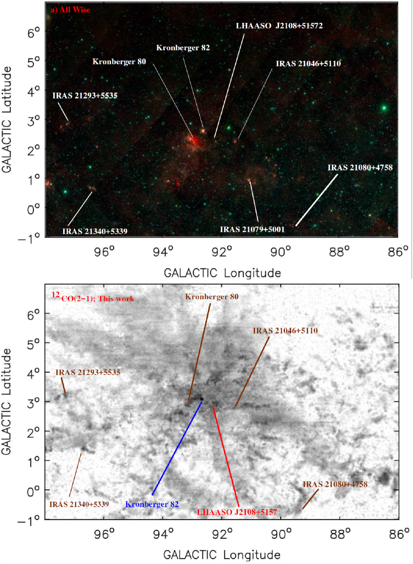
Figure 1: Top: All WISE RGB (22$\mu$m +4.6$\mu$m +3.4$\mu$m) image of COB7-MC centred at l = 93^∘ and b = +03^∘. No clear counterpart is observed for J2108, although Kronberger 80, Kron 82, and IRAS 21046 are predominant in its neighbourhood. Down: The low resolution total flux integrated ¹²CO(2$\rightarrow$1) map (Nishimura et al., 2020) discussed in the text. The brightest point corresponds to Kron 82 (blue marker). No clear condensation is observed on the J2108 position, but the vicinity is surrounded by molecular gas. Some IRAS sources and objects related to star-forming and star clusters are labelled for identification.

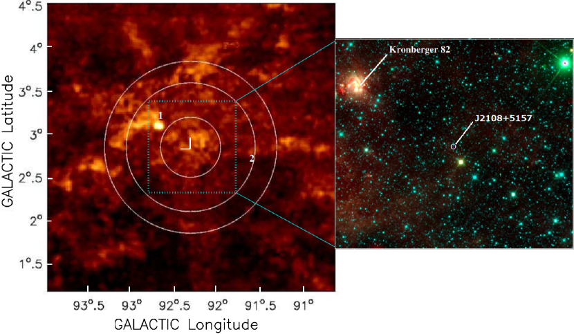
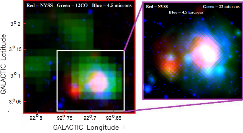
Figure 2: Top: Same as Fig. 1, but in a 3 square degree field and centred in J2108 (marks): $\alpha$(2000) = 21^h08^m36^s; $\delta$(2000) = +51^∘57’00” for the ¹²CO(2$\rightarrow$1) emission. The diameters of the circles are 0.7, 1.5, and 2^∘ respectively. The regions related to Kron 82 (peak) and IRAS 21046+5110 are labelled as 1 and 2 respectively. All WISE RGB image (red = 22$\mu$m, green = 4.6$\mu$m, and blue = 3.4 $\mu$m) with a size of $\sim$ 1^∘ is shown as an inset. The small circle shows the position of J2108. Down: A zoom of the zone labelled as 1 in the top left panel (Kron 82). This RGB image is NVSS (RC at 20 cm in red), our ¹²CO (2-1) data (in green), and the Spitzer–IRAC 4.5 $\mu$m image (in blue). Another RGB image (red = NVSS; green = WISE 22 $\mu$m; and blue = Spitzer–IRAC 4.5 $\mu$m) is shown as an inset. Thus, Kron 82 is the more prominent object across wavelengths. There are no RC or IR emissions in the vicinity of J2108 location.

2 Sources Overview

2.1 Cygnus OB7

The Cygnus constellation contains several prominent HII regions, OB associations, and massive star clusters. Particularly, the Cygnus OB2 association is notable in the Galaxy because of the large number of massive stars, including Wolf-Rayets. Reipurth & Schneider (2008) presented an extinction map of the Cygnus molecular cloud complex, providing a complete overview of the star forming regions and young star clusters in Cygnus showing (see their Fig. 1). Their map includes Cygnus-X, the North American Nebula, the Pelican Nebula, and COB7- MC, all of them lying within a distance from the Sun ranging from 600 pc (North American and Pelican Nebula) to 1.7 kpc (Cygnus-X; Schneider et al. (2006)). Considering a distance of 800 pc Humphreys (1978); Dobashi et al. (1994); Dobashi, Bernard, & Fukui (1996) estimate a total mass of M $\sim$ 1 $\times$ 10⁵ M_⊙.

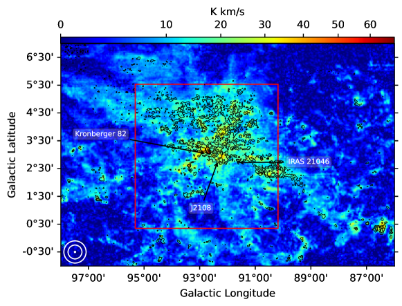
Figure 3: ¹²CO(J=2$\rightarrow$1) map for COB7-MC (Nishimura et al., 2020) with the ¹³CO(J=2$\rightarrow$1) emission overlaid as black contours for different representative velocities ranges (this work). The positions of Kron 82, IRAS 21046, and J2108 are indicated with black arrows. The red square represents the field in Fig. 4 within which only HI emission was observed. The beams of LHAASO (0.8^∘ and 0.5^∘) and OPU (2.7’) are shown as white circles in the bottom left corner.

The large-scale regions of COB7 were surveyed in the infrared by WISE and also partially by GLIMPSE 360 (3.6$\mu$m and 4.5$\mu$m). We show the the WISE RGB image (22$\mu$m + 4.6$\mu$m + 3.4$\mu$m) in Fig. 1 (top). Some regions, mainly associated with IRAS sources, are labelled for their easy identification. In the bottom panel of the same figure we also show an image of the ¹²CO(J=2$\rightarrow$1) emission obtained with the 1.85 m radio telescope at Osaka Prefecture University (OPU). These observations were presented by Nishimura et al. (2020), however, they did not perform any analysis of the observations. The morphology of the emission is compatible with the distribution of the emission in the low-resolution ¹³CO(J=1$\rightarrow$0) observations (angular resolution of $\sim$ 3’) performed with the two 4m-millimetre telescopes of the Nagoya Observatory (Dobashi et al., 1994, see also Fig. 1 of Dobashi et al. 2018). The ¹²CO(J=2$\rightarrow$1) map is the same one investigated and described in this work by adding the corresponding $,^{13}$CO(J=2$\rightarrow$1) observations (see § 3).

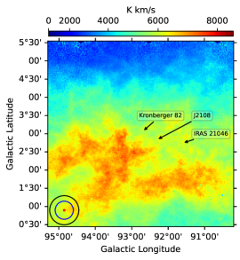
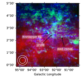
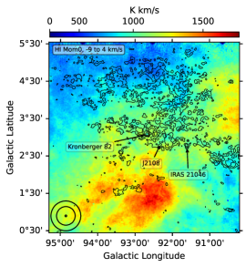
Figure 4: Left: DRAO HI (21 cm) line image with J2108 at the center ($\alpha$(2000) = 21^h08^m36^s; $\delta$(2000) = +51^∘57’00”). The image was generated considering an integration range between –150 and 50 km s^-1. The HI image does not cover the whole CO field compared with Fig. 3. Center: RGB (red = DRAO 21 cm, green = ¹³CO(J=2$\rightarrow$1), blue = ¹²CO(J=2$\rightarrow$1)) image from the same field at the left panel. Right: HI (21 cm) line emission, integrated between –9 and 4 km s^-1 in the same field of view as the left panel, with ¹³CO(J=2$\rightarrow$1) emission overlaid in black contours (integrated between –100 to 80 km s^-1). The size of images is 5$\times$5 degrees. The y-axis and x-axis are Galactic latitude and longitude, respectively. The beams of LHAASO (0.8^∘ and 0.5^∘) and OPU (2.7’) are shown in circles at the bottom left.

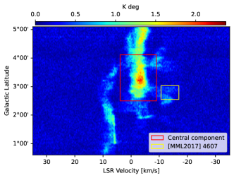
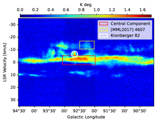
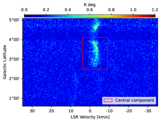
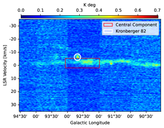
Figure 5: Galactic longitude and latitude ¹²CO(J=2$\rightarrow$1) (top panels) and ¹³CO(J=2$\rightarrow$1) (bottom panels) emission maps as function of the V_LSR for J2108 vicinity. Data have been integrated into an interval of 0.5^∘ around the centre location of LHAASO J2108+5157: $l$ = 92.31, and $b$ = 2.84. The molecular cloud in the red rectangle is [FKT-MC]2022 (V_LSR $\sim$ –3 km s^-1), and the yellow rectangle covers MML (V_LSR $\sim$ –13 km s^-1), which is not observed at ¹³CO(J=2$\to$1). The cloud just above the red rectangle in both right panels is Kron 82 (V_LSR $\sim$ –7 km s^-1), which was not considered in the [FKT-MC]2022 size calculation (see § 5.1.2).

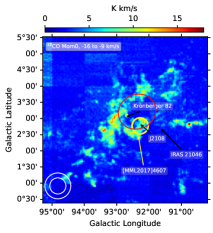
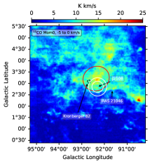
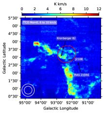
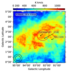
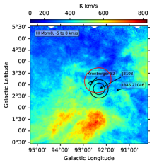
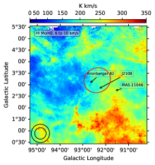
Figure 6: Maps of moment 0 for ¹²CO (top panels) and HI (bottom panels) emissions. The range of integration in LSR velocity corresponds to the FWHM for the three spectral components of ¹²CO emission shown in Fig. 7. Except for central panels, the beams of LHAASO (0.8^∘ and 0.5^∘) are shown as circles at the bottom left. For the central panels, these beams are located at centre. The yellow (top-left) and red circles (all panels) correspond to the sizes of MML and [FKT-MC]2022 respectively. Both clouds are inside the resolution of LHAASO. An intersection zone is observed at the center of J2108. In Fig. 5, Kron 82 only shows emissions in the galactic longitude maps. Nevertheless, we remove the associated pixels (small black dashed circle at top-centre panel) in the computing of [FKT-MC]2022 size (see §5.1.2). Therefore, the FKT-MC]2022 size does not include Kron 82 emission.

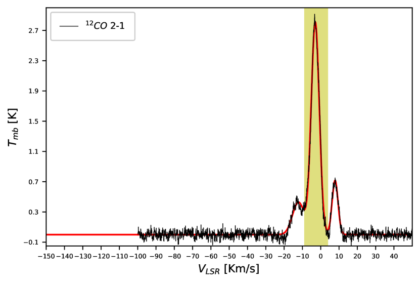
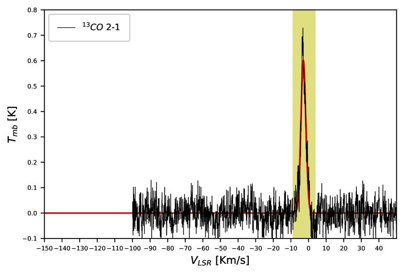
Figure 7: Total integrated spectra for the OPU ^12,13CO(J=2$\to$1) and DRAO HI (21 cm) lines observations. The spectra were obtained for the red region depicted in Fig. 6. The emission map for the different components is shown in Fig. 6 for CO and HI. The yellow hatched areas fill the velocity range of the main component for ^12,13CO(J=2$\to$1). This range covers part of the main (more intense) for the HI with part of the following right component (see text for details). The components to the left and right of the central line for ¹²CO(J=2$\to$1), correspond to COB-7 molecular gas at different LSR velocities.

2.2 LHAASO J2108+5157

J2108 is located at $\alpha$(2000) = 21^h08^m52.8^s; $\delta$(2000) = +51^∘57’00” or l = 92.30^∘; b = 2.84^∘. The LHAASO observatory detected very high-energy gamma-ray emission in the energy ranges of 25 to 100 TeV and above 100 TeV at 9.5 $\sigma$ and 8.5 $\sigma$ respectively, with an angular resolution of $\sim$0.3^∘(Cao et al., 2021a). Therefore, it was postulated to be a PeVatron candidate (Cao et al., 2021a, b). The observed morphology is circular with an upper limit on the source size of 0.26 degrees with 95% confidence level covering a flux at 100 TeV of 0.38$\pm$0.09 CU . A power law spectrum with a spectral index of –2.83 best describes the spectral energy distribution. The gamma-ray source has not been identified, no distance has been determined, and there is no known TeV counterpart. To date, neither HAWC (sensitive to a few hundred GeV to above 100 TeV; Albert et al. 2020b) nor the Tibet-AS$\gamma$ Observatory (sensitive to energy above 100 TeV; Albert et al. 2020b) has reported emission at that energies.

The NASA-FERMI source 4FGL J2108.0+5155 at J(2000) RA = 317.02^∘ and Dec = 51.92^∘) has a separation of 0.13^∘ from the sub-PeV emission observed by LHAASO being the only gamma source in the vicinity(Abdollahi et al., 2020). A symmetric Gaussian describes the morphology of the GeV emission with a width of 0.48^∘ (Cao et al., 2021b). Assuming that the spectral energy distribution of the source extends to the VHE energies, extrapolating the spectrum to these energies leads to a flux lower by a factor of 10 than the one observed by LHAASO(Abdollahi et al., 2020; Cao et al., 2021b). The nearest X-ray source, an eclipsing binary RX J2107.3+5202 (Motch et al., 1997), is separated by 0.3^∘.

According to LHAASO, the gamma-ray emission from J2108 can be described by leptonic and hadronic origins, although there are no known SNRs and PWNe within 0.8^∘ of the centre of the sub-PeV emission. Even though there is no known pulsar in this region to support the leptonic scenario, the possible contribution of a yet unknown pulsar cannot be ignored. On the other hand, Cao et al. (2021b) suggest an association with the molecular cloud [MML2017]4607 (MML hereafter) with radius = 0.24^∘, mass = 8469 M_⊙, and distance $\sim$ 3.3 kpc (3.28 kpc; Miville-Deschenes, Murray, & Lee, 2017), favouring the hadronic emission. This result is based on the ¹²CO(J=1$\rightarrow$0) survey of Dame, Hartmann, & Thaddeus (2001), where the optical depth ($\tau$) is optically thick and does not include emission from inner regions. In any case, although there is no consensus on the distance, it is worthwhile to make the same suggestion but considering optically thin observations, high-density tracers of clumps, and other distances to COB7-MC such as those reported by Humphreys (1978); Schneider et al. (2006) from 800 pc to 1.7 kpc instead of 3.3 kpc.

A lepto-hadronic model in sub-PeV emission environments associated with giant molecular clouds without a strong pulsar or supernova remnant as in J2108 is described by Kar & Gupta (2022). This model assumes collisionally accelerated electrons and protons injected into the local interstellar medium from past supernova explosions thousands of years ago. This model can be tested by combining high-resolution HI (unavailable) with X-rays (leptonic emission), shocked HII gas tracers such as H$\alpha$, forbidden lines (optical supernova remnants), and radio-continuum (RC) observations at 20 cm (synchrotron and pulsars) and 3.6 cm (Bremsstrahlung). Successful examples of the discovery, confirmation, and study of supernova remnants interacting with molecular clouds include SN 1006, RX J1713.7-3946, 3C400.2, G350.0-2.0, IC443 G352.7-0.1, and others (e.g Sano et al., 2022; Fukui et al., 2021, 2012; Erging et al., 2017; Karpova et al., 2016; Toledo-Roy et al., 2014; Jiang et. al, 2010; Schneiter, de la Fuente, & Velázquez, 2008; Albert et al., 2007; Ambrocio-Cruz, Rosado, & de La Fuente, E., 2006, and references therein). Detecting a supernova (and its remnant) in J2108 is crucial for understanding the contribution of leptonic (and possibly hadronic) emission to the observed sub-PeV emission.

3 Observations

We report observations of COB7-MC carried out with the 1.85 m radio-telescope (Nishimura et al., 2020; Onishi et al., 2013) of the OPU at Nobeyama Radio Observatory. The observations were conducted from February to May 2011. A receiver for observation at 230 GHz was used to produce ¹²CO(J=2$\rightarrow$1) and ¹³CO(J=2$\rightarrow$1) maps with an angular resolution of $\sim$3$\arcmin$ covering a spectral window from -100 to 80 km s^-1 in the local standard of rest (LSR). The data were calibrated with the standard procedure used for previous data sets obtained with the same telescope (Onishi et al., 2013; Nishimura et al., 2015). The RMS value of the noise is $\sim$0.3 K at a velocity resolution of 0.3 km s^-1.

We retrieve atomic hydrogen (HI) 21 cm line observations from the Dominion Radio Astrophysical Observatory (DRAO) archives (Taylor et al., 2003), at a Galactic longitude and latitude that includes the position of J2108. These observations were taken on August 20, 2001, with a resolution of 1 arcminute at 1420 MHz. The data set is projected into a 1024$\times$ 1024, 18 arcsec pixel mosaic image, with 0.82 km s^-1 velocity channels. The RMS noise of the brightness temperature for an empty channel is between 2.1 and 3.2 K.

4 Methodology: The density of nucleons; n(H)

Assuming that no external astronomical source such as the PeVatron is found in the region where the sub-PeV emission is observed, a molecular cloud or clump in a molecular environment, where the neutral pion decay process may occur, is a good candidate to produce this (hadronic) emission. In this scenario, the hadronic contribution (N${}^{\rm had}_{\gamma}$) may be calculated from the observed total flux of gamma-ray emission.

$$\rm{N^{\rm obs}_{\gamma}=\rm{N^{\rm had}_{\gamma}}+N^{\rm lep}_{\gamma}},$$ (1)

as

$$\rm{N^{had}_{\gamma}}=\rm{N^{obs}_{\gamma}}-\rm{N^{lep}_{\gamma}}\propto c~{}n(\rm{H})N_{\rm P}(\rm CR),$$ (2)

with:

$$\rm{N^{\rm lep}_{\gamma}}\propto\rm{N^{\rm obs}_{X-Ray}\Bigg{[}\frac{N(CMB)}{B^{2}}\Bigg{]}}.$$ (3)

In these equations, c is the speed of light in vacuum, N_γ is a differential flux $\frac{dN}{dE}$ corresponding to total emission (hadronic and leptonic) expressed in units of $\rm TeV^{-1}\ cm^{-2}\ s^{-1}$, n(H) is the numeric density of the nucleons (protons) involved in the hadronic emission (N${}^{\rm had}_{\gamma}$), N_P(CR) corresponds to cosmic ray counts (CR) in hadronic emission (e.g Amenomori et al., 2021b; Ackermann et al., 2011), N${}^{\rm obs}_{\rm X-ray}$ is the observed X–ray count, N(CMB) is the photon density from the cosmic microwave background, and B is the ISM magnetic field. The X–ray emission is required to calculate the leptonic contribution using the inverse Compton effect. The Eq. 2 is supported by standard models (Kelner, Aharonian, & Bugayov, 2006) and has been used effectively to SNR RX J1713.7-3946 (Fukui et al., 2021, 2012). Observations of leptonic emission can constrain the value of N${}^{\rm lep}_{\gamma}$ (e.g. X–rays; Fukui et al., 2021, and references therein), and n(H) can be calculated from the total proton column density, N(H), obtained from CO and HI observations as

$$\rm N(H)=2N(H_{2})+N(HI),$$ (4)

where N(H₂) is calculated from the CO column density, N(CO). To obtain a complete understanding of the protons in the ISM, the column density of HI, N(HI), must be included in this equation(see Fukui et al., 2021, 2012; Ade et al., 2011, and references therein). Then, in the standard way (see Appendix 1)

$$\rm N(H_{2})=5\times 10^{5}\ N\left({}^{13}CO\right),$$ (5)

$$\left[\frac{N({\rm HI})}{\rm cm^{-2}}\right]=1.823\times 10^{18}\left[\frac{\int T_{\rm MB}^{HI}dv}{\rm K\ km\ s^{-1}}\right],$$ (6)

where N(¹³CO) is the ¹³CO column density (derived from J=2$\rightarrow$1 line), and $T_{\rm MB}^{HI}$ is the brightness temperature averaged over the main beam as a result of a Gaussian fit of the HI emission spectrum. Using the relationship between column and number density and assuming a constant number density of the cloud, we can estimate the number density as follows:

$${\rm n(H)}=l^{-1}\rm{N(H)},$$ (7)

where $l$ is the physical size of the region under consideration.

The latter requires a careful search for the molecular clump and the determination of a suitable size, mass and distance, because the calculation of these parameters is fundamental for determining the density of the nucleons. This computing is particularly hard for COB7 due to its complex morphology, since the size, morphology (mainly), and distance are significant sources of uncertainty.

5 Results and Discussion

In Fig. 2 (top-left) we present close-up of the ¹²CO(J=2$\to$1) images from Fig. 1, but centred on J2108. The circles cover regions of interest (ROIs) with diameters of 0.7, 1.5, and 2.0 degrees, where all source candidates for PeVatron (Cao et al., 2021b) including IRAS 21046+5110 are located. Kron 82 and IRAS 21046 are marked 1 and 2, respectively, and are the closest star clusters to J2108. The WISE RGB image (red = 22$\mu$m, green = 4.6$\mu$m blue = 3.4$\mu$m) is shown as a one-degree square ($\sim$ four times the upper limit of LHAASO KM2A PSF for J2108 Cao et al. (2021b) inset in the upper right panel. The Kron 82 emission stands out, and IRAS 21046 does not appear in the field. In the images from WISE, IRAS 21046 is fainter than Kron 82, its emission is not as spectacular, and it is further away from J2108 than Kron 82 (at a distance of $\sim$ 0.7^∘ versus $\sim$ 0.4^∘; a reason to be discarded by Cao et al. (2021b).

There are no precise molecular emissions and counterparts in the centre of J2108, particularly in the upper limits emission extension circles at the upper edge at GeV (NASA-FERMI) and sub-PeV (LHAASO) emissions (see Fig. 4 of Cao et al., 2021b, which includes observations from Dame, Hartmann, & Thaddeus 2001). Kron 82 shows a 20 cm radio continuum (RC; Taylor et al. (2003)) in agreement with the 20 cm RC emission from NVSS (Condon et al., 1998), but no CO emission is observed.

In contrast, Kron 82 is a bright source on the map in our OPU ^12,13CO(J=2$\to$1) emission. Kron 82 is the closest optical/radio counterpart to J2108. If the Cygnus OB2 star cluster is the PeVatron in the Cygnus cocoon, it is worth investigating and confirming whether Kron 82 could be the counterpart of J2108. Therefore, we reinforce the idea that a molecular clump or Kron 82 is the gamma-ray emission candidate. Nevertheless, there is no extended X-ray evidence in the literature for stellar winds or similar processes in massive stars at several degrees.

In Fig. 2 (bottom left) we show a zoom of Kron 82 in an RGB image (NVSS in red, OPU ¹²CO(J=2$\to$1) in green, and Spitzer-IRAC at 4.5$\mu$ in blue). As an inset (bottom right), another RGB image (NVSS in red, WISE 22$\mu$m in green, and Spitzer–IRAC 4.5$\mu$m in blue) is shown. Kron 82 is the only object with NVSS emission in the vicinity of J2108 at least in several degrees.

We present the OPU ^12,13CO(J=2$\to$1) study and gamma-ray modelling for Kron 82 in Appendix  2. This appendix shows that although Kron 82 requires a cosmic-ray energy (proton) of $\sim 10^{45}$ erg to produce the reported LHAASO emission, it is located outside the radial angular extension of J2108. Thus, discarding Kronberger 80 (distance $\sim$ 5 kpc; Cao et al. 2021b), IRAS 21046 (distance $\sim$ 600 pc; Kumar, Keto, & Clerkin 2006) and Kron 82 (due to their stellar content, mass and angular separation from J2108; distance $\sim$ 1.6 kpc), a molecular cloud near J2108 could be the best option to produce the observed sub-PeV emission. However, this molecular cloud could not be MML (distance of $\sim$ 3.3 kpc), as stated in § 2.2.

5.1 Cygnus OB7 and the vicinity of LHAASO J2108+5157

5.1.1 HI and CO emission

In Fig. 3, we show the integrated ¹²CO(J=2$\to$1) emission (in colour) in the velocity range between -100 and 80 km s^-1) with the integrated ¹³CO(J=2$\to$1) emission (same velocity range) superimposed as black contours. The ¹³CO(J=2$\to$1) emission predominates in the north, especially in the NE, and is almost absent in the south, where the ¹²CO(J=2$\to$1) emission remains. The red square marks the region shown in Fig. 4, the only one with HI reported. In this Fig. we show the DRAO HI 21 cm map (left), an RGB image (center) with DRAO 21 cm in red, ¹³CO(J=2$\rightarrow$1) in green, ¹²CO(J=2$\rightarrow$1) in blue, and a HI 21 cm map integrated between –9 and 4 km s^-1 (corresponding to the brightest spectral component of the region; right), overlaid with the ¹³CO(J=2$\to$1) emission. The positions of J2108 (LHAASO) and Kron 82 are labelled. The extent of HI and CO gas is huge, but neither J2108 nor Kron82 have a clear clump or counterpart in HI. Remarkably, we observed a strong anti-correlation between the ¹³CO(J=2$\to$1) and the HI maps. Furthermore, the ¹²CO(J=2$\to$1) emission is more extended than the ¹³CO(J=2$\to$1).

To identify molecular clouds near J2108, we show ^12,13CO(J=2$\to$1) maps of Galactic latitude and longitude as a function of V_LSR in Fig. 5. We detect MML at V_LSR $\sim$ –13 km s^-1 (yellow rectangle) and a gas parcel with V_LSR $\sim$ –3 km s^-1, called central component and enclosed with a red rectangle (see § 5.1.2). We observe this cloud ([FKT-MC]2022 below) at ¹³CO(J=2$\to$1) (optically thin emission), unlike MML. Therefore, [FKT-MC]2022 and MML are molecular clouds near J2108, but [FKT-MC]2022 is detected by its optically thin emission.

We can see in Fig. 5 the ¹²CO(J=2$\to$1) emission associated with Kron 82 at V${}_{\rm LSR}\sim-6$ km s^-1 (white circle). To exclude this contribution, we integrate between -5 and 0 km s^-1 and present a ¹²CO(J=2$\to$1) moment-0 map in the top central panel of Fig 6. We identify [FKT-MC]2022 in the central region of the map by fitting a 2-dimensional Gaussian. We estimate a central position of $l=$ 92.4^∘ and $b=$ 3.2^∘ with corresponding standard deviations $\sigma_{l}$ = 0.50^∘ and $\sigma_{b}$ = 0.45^∘ with a P.A. = 19 deg. Using these fitted values, we estimate the angular extent of the cloud at FWHM from the central position, shown as a red ellipse in Fig 6. Finally, if we consider a beam of 2.7$\arcmin$ $\times$ 2.7 $\arcmin$, we obtain a deconvolved size of 1.1 $\pm$ 0.2^∘ (Nishimura et al., 2020).

In Fig. 6 we show moment 0 maps for ¹²CO(J=2$\to$1) and HI emissions for three different ranges of LSR velocity: –16 to –9, –5 to 0 and 6 to 10 km s^-1. The yellow circle in the top-left panel shows the vicinity of J2108 at 0.5^∘ where MML is marked. The red ellipse covers [FKT-MC]2022 to its full extent (size of 1.1 ^∘) in all panels. Except in the central panels, we show the two “beam sizes” of LHAASO at 0.8^∘ and 0.5^∘ the bottom left, respectively. In central panels, these “beams” appear centred in J2108. Comparing the position of [FKT-MC]2022 with the LHAASO beams and MML, [FKT-MC]2022 can also be considered a candidate for producing the sub-PeV emission.

We show in Fig. 7 the average spectra of the ^12,13CO and HI line emissions obtained from the angular extension of [FKT-MC]2022. The ¹²CO spectrum shows three main velocity components, denoted as left, centre (the brightest), and right (see Tab. 1). We have performed a Gaussian fit for the three components. At V${}_{\rm LSR}\approx$ –2.9 km s^-1 to –3.0 km s^-1, the central component is detected with a signal-to-noise ratio of $\sim$ 15. This brightest component is the only one detected in the spectrum of ¹³CO with an signal-to-noise ratio of $\sim$ 13. As a result, as shown in Fig. 6, the left and right components are ¹²CO gases with different velocities, respectively. The spectrum of HI has a complex structure and several velocity line components; a Gaussian curve with five components was fitted to this spectrum. The brightest line (main line) and the next one to the right cover the three lines observed in ¹²CO and the main line in ¹³CO. We can explain this behaviour by the fact that these two HI lines are one spectral line that suffers self-absorption (e.g. Jackson et. al, 2002). All fitting parameters are shown in Tab. 1.

After discovering [FKT-MC]2022 at V${}_{\rm LSR}\sim-3$ km s^-1, and calculating its angular extension, we estimate its physical parameters, confirming through modeling the amount of energy required to produce the gamma-ray emission detected by LHAASO. Finally, both clouds, MML and [FKT-MC]2022, are compared to one another.

5.1.2 [FKT-MC]2022 Physical parameters

Table 1: Fitted parameters of HI, ¹²CO(J=2$\rightarrow$1) and ¹³CO(J=2$\rightarrow$1) emission via Gaussian fit. The main beam (MB) averaged peak temperature ($T^{p}_{\rm MB}$) uncertainties are only due to rms noise. Velocity channel resolutions are used to show the LSR velocity (V_LSR) and FWHM ($\Delta V$) uncertainties.

Spectral	Size	VLSR	$\Delta V$	$T^{\rm p}_{\rm MB}$	$\int T_{\rm MB}dv$
Line	[deg]	$\rm km\ s^{-1}$	$\rm km\ s^{-1}$	[K]	[$\rm K\ km\ s^{-1}$]
12CO 2-1 (left)	1.1 $\pm$ 0.2	–12.19 $\pm$ 0.08	7.55 $\pm$ 0.19	0.43 $\pm$ 0.01	3.45 $\pm$ 0.10
12CO 2-1 center (main)	1.1 $\pm$ 0.2	–2.98 $\pm$ 0.01	5.21 $\pm$ 0.02	2.80 $\pm$ 0.01	15.54 $\pm$ 0.08
12CO 2-1 (right)	1.1 $\pm$ 0.2	7.84 $\pm$ 0.03	3.78 $\pm$ 0.06	0.72 $\pm$ 0.01	2.88 $\pm$ 0.06
13CO 2-1 (main)	1.0 $\pm$ 0.2	–2.91 $\pm$ 0.03	3.31 $\pm$ 0.07	0.60 $\pm$ 0.01	2.12 $\pm$ 0.06
HI (main)	1.1 $\pm$ 0.2	–10.18 $\pm$ 0.11	15.01 $\pm$ 0.25	108.46 $\pm$ 0.90	1740.37 $\pm$ 32.21
HI (right to main)	1.1 $\pm$ 0.2	4.42 $\pm$ 0.15	9.76 $\pm$ 0.30	58.62 $\pm$ 1.32	608.88 $\pm$ 23.34

In Tab. 2 we present the relevant parameters of the ^12,13CO and HI fitted spectra (see Fig. 7) used to estimate the physical parameters of [FKT-MC]2022. Based on a gas region of 1.1^∘ size (red ellipse in Fig. 6), we examine only the central component of the ¹²CO(J=2$\to$1) spectrum and the single component fit for the ¹³CO(J=2$\to$1). In the case of the HI emission, we focus on the V_LSR range similar to the ^12,13CO(J=2$\to$1) emission (between $\sim$ –4 and 9 km s^-1), which corresponds to the velocity range considered only in the main-beam averaged brightness temperature (see Fig. 7)

We estimate T_ex from Eq. 1.2 using the ¹²CO(J=2$\to$1) emission line, assuming it is optically thick. The result with a mean value of $\approx$ 7.0 K is shown in Tab. 2. This value agrees with the lower value given by Schneider et al. (2006) for several clumps in Cygnus-X (7-28 K) and is similar to the temperature (10 K) given by Dobashi et al. (2014) for the core L1004E of the dark nebula LDN 1004 in the COB7- MC.

Considering the local thermodynamic equilibrium (LTE) conditions for the ^12,13CO(J=2$\to$1) emission, assuming an optically thin emission for ¹³CO, and using the main-beam peak brightness temperature of the fitted spectra (see Tab. 2), we calculate the optical depth $\tau^{13}_{\rm CO}$ from the ¹³CO emission according to Eq. 1.3. Assuming a standard value for the isotopic abundance ratio of $\rm{}^{12}CO/^{13}CO\approx 60$ for the local interstellar medium (Langer et al., 1993), we estimate the optical depth of ¹²CO as $\tau^{12}_{CO}$ = 60 $\tau^{13}_{\rm CO}$. The estimated optical depths $\tau^{13}_{\rm CO}$ and $\tau^{12}_{\rm CO}$ can be found in Tab. 2.

We calculate the column densities of ^12,13CO using Eqs. 1.5 and 1.6 introducing the corresponding values presented in Tab. 2. The HI column density is determined using Eq. 6 assuming optically thin emission. We show the estimated column densities for all emissions in Tab. 3. We obtain a mean value of N(¹³CO) $\approx$ 1.8 $\times$ 10¹⁵ cm^-2, similar to the lower values reported by Schneider et al. (2006) for Cygnus-X (0.6 – 6.9 $\times 10^{16}$ cm^-2). The H₂ column density is calculated from ^12,13CO using Eq. 1.7. The results are shown in Tab. 3. Mean values of N(${\rm H_{2}}$) = 3.1 $\times$ 10²¹ and 9.1 $\times$ 10²⁰ cm^-2 are obtained from ¹²CO(J=2$\to$1) and ¹³CO(J=2$\to$1) emissions, respectively. These values agree in order of magnitude with those reported for Cygnus-X (Uyaniker et al., 2001). Finally, we estimate the total proton column density $N(\rm H)$ using both ^12,13CO(J=2$\to$1) emission (separately) and Eq. 4. The calculated values are shown in Tab. 4. Nucleon column densities of $\rm N(H)$ = $3.7\times 10^{21}$ or $8.1\times 10^{21}$ cm^-2 are obtained with ¹²CO(J=2$\to$1) or ¹³CO(J=2$\to$1) emission, respectively.

The distance of 3.3 kpc to MML molecular cloud candidate (Cao et al., 2021b) was estimated using the rotation curve of Brand & Blitz (1993) by Miville-Deschenes, Murray, & Lee (2017). For comparison, using the ¹³CO(J=2$\to$1) V_LSR of -2.9 km s^-1, we estimate a (far) kinematic distance of 1.7${}^{+0.5}_{-0.7}$ kpc to [FKT-MC]2022 using the same rotation curve. The latter implies a physical size of the cloud of 33.4 $\pm$ 11.5 pc using a small angle approximation with an angular size of 1.1^∘. Substituting the size of the cloud into Eq. 7, we calculate the corresponding n(H) via ^12,13CO emission using both distances (3.3 and 1.7 kpc). We present the estimated n(H) values in Tab. 4 using both distances to MML and [FKT-MC]2022. Using ¹³CO(J=2$\to$1) and ¹²CO(J=2$\to$1) emissions we obtain nucleon number densities of $\rm n(H)\sim$ 37 and $\sim$ 80 cm^-3, respectively. In addition, using the rotation curve of Reid et al. (2014), we estimate a kinematic distance of $\sim$ 1.2$\pm$0.6 kpc, and a nucleon density of $\sim$ 52$\pm$28 $\rm cm^{-3}$ (via ¹³CO emission), comparable within uncertainties to that using a distance of 1.7 kpc.

Finally, for [FKT-MC]2022, we estimated the average number density of molecular hydrogen n$({\rm H_{2}})$ for both ^12,13CO emissions using the Eq. 7 using the estimated column density of H₂ in Tab. 3. The total mass of the molecular gas M($\rm H_{2}$) is obtained as follows:

$$M({\rm H_{2}})=\frac{4}{3}\pi(2\mu m_{H})R^{3}n({\rm H_{2}}),$$ (8)

where $m_{H}=$ 1.67 $\times 10^{-24}$ g is the mass of the hydrogen atom and a molecular weight $\mu=$ 1.36 (Miville-Deschenes, Murray, & Lee, 2017; Takekoshi et al., 2019) is considered. We estimate the virial mass $\rm M_{vir}$ of the molecular cloud with (Garay and Lizano, 1999) as:

$$M_{\rm vir}=210\left[\frac{R}{\rm pc}\right]\left[\frac{(\Delta\rm V)}{\rm kms^{-1}}\right]^{2},$$ (9)

where we use the FWHM velocity width $\Delta\rm V$ of the ^12,13CO fitted spectra from Tab 2. The calculated $\rm H_{2}$ number densities and masses are shown in Tab. 5. Comparing this mass to the virial mass, it appears that [FKT-MC]2022 is close to virial equilibrium. The mean value of n(${\rm H_{2}}$) $\sim$ 20 cm^-3 for both ^12,13CO emissions is similar to the mean value of $\sim$ 24 cm^-3 given in the ¹²CO(J=1$\rightarrow$0) catalogue of molecular clouds by Miville-Deschenes, Murray, & Lee (2017), including MML. For MML using Eq. 23 of these authors: n(${\rm H_{2}}$) = 12 cm^-3; (see Tab. 5), which implies a density of nucleons (without HI) n(H) = 2n(${\rm H_{2}}$) = 24 cm^-3.

Table 2: Values used for the column density analysis.

Species	Diameter	$T_{\rm MB}^{\rm peak}$	$\int T_{\rm MB}dV$	$T_{\rm ex}$	$\tau^{12,13}_{\rm CO}$
	[deg]	[K]	[K km s-1]	[K]
HI	1.1 $\pm$ 0.2	–	1018.45 $\pm$ 21.63	–	–
12CO 2-1	1.1 $\pm$ 0.2	2.80 $\pm$ 0.04	15.54 $\pm$ 0.08	7.16 $\pm$ 0.05	13.91 $\pm$ 1.23
13CO 2-1	1.1 $\pm$ 0.2	0.60 $\pm$ 0.05	2.12 $\pm$ 0.06	7.16 $\pm$ 0.05	0.23 $\pm$ 0.02

Table 3: Estimated column density (N) of HI, ¹²CO, ¹³CO, and $\rm H_{2}$ for [FKT-MC]2022. The 12 and 13 labels correspond to the respective CO emission used in the calculations.

Diameter	$N(\rm^{13}CO)$	$N(\rm^{12}CO)$	$N(\rm HI)$	$N^{\rm{}^{12}CO}(\rm H_{2})$	$N^{\rm{}^{13}CO}(\rm H_{2})$
deg	[$10^{15}$ cm-2]	[$10^{17}$ cm-2]	[$10^{21}$ cm-2]	[$10^{21}$ cm-2]	[$10^{20}$cm-2]
1.1 $\pm$ 0.2	1.8 $\pm$ 0.1	1.7 $\pm$ 0.2	1.9 $\pm$ 0.4	3.1 $\pm$ 0.9	9.1 $\pm$ 2.7

Table 4: Estimated nucleon (H = 2H₂ + HI) column (N) and numeric (n) densities of the molecular cloud [FKT-MC]2022 using distances of 1.7 kpc and 3.3 kpc. The 12 and 13 labels correspond to the respective CO emission used in the calculations.

Diameter	$N^{12}(\rm H)$	$N^{13}(\rm H)$	$n^{12}(\rm H){\scriptstyle(1.7kpc)}$	$n^{13}(\rm H){\scriptstyle(1.7kpc)}$	$n^{12}(\rm H){\scriptstyle(3.3kpc)}$	$n^{13}(\rm H){\scriptstyle(3.3kpc)}$
$[\rm deg]$	[$10^{21}\rm cm^{-2}$]	[$10^{21}\rm cm^{-2}$]	[$\rm cm^{-3}$]	[$\rm cm^{-3}$]	[$\rm cm^{-3}$]	[$\rm cm^{-3}$]
1.1 $\pm$ 0.2	8.1 $\pm$ 1.9	3.7 $\pm$ 0.7	80 $\pm$ 34	37 $\pm$ 14	42 $\pm$ 10	19 $\pm$ 3

Table 5: Parameters of the molecular cloud [FKT-MC] 2022 and comparing with [MML2017]4607

Source	VLSR	$D$	Distance	$n({\rm H_{2}})$	$M_{\rm vir}({\rm H_{2}})$	$M({\rm H_{2}})$	$M(\rm HI+H_{2})$	Projected Size
	[$\rm km\ s^{-1}$]	[deg]	[kpc]	[$\rm cm^{-3}$]	[$10^{4}M_{\odot}$]	[$10^{4}M_{\odot}$]	[$10^{4}M_{\odot}$]	[deg]
MML	-13.71	0.5	3.3	12.26	–	0.84	–	0.5 at 3.3 kpc
FKT-MC (12CO)	-3.0 $\pm$ 0.1	1.1 $\pm$ 0.2	1.7 $\pm$ 0.6	31 $\pm$ 14	9.5 $\pm$ 0.1	3.0 $\pm$ 1.4	3.6 $\pm$ 1.6	1.1 at 1.7 kpc
FKT-MC (13CO)	-2.9 $\pm$ 0.1	1.1 $\pm$ 0.2	1.7 $\pm$ 0.6	9 $\pm$ 4	3.8 $\pm$ 0.2	0.9 $\pm$ 0.4	1.5 $\pm$ 0.6	1.1 at 1.7 kpc

5.1.3 Modelling gamma-rays

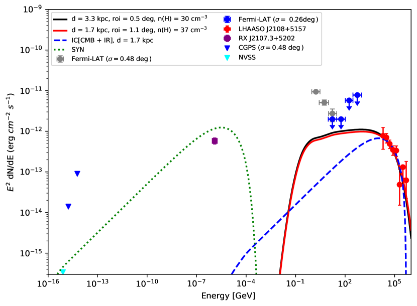
Figure 8: Spectral energy distribution of the LHAASO J2108+5157 region. Red circles are from the LHAASO observatory (Cao et al., 2021b). The grey and blue circles are GeV fluxes and the upper limit reported by the Fermi-LAT observatory, respectively (Abdollahi et al., 2020, and references therein). The purple square is the ROSAT X-ray source RX J2107.3+5202 (Motch et al., 1997). The blue and cyan triangles are radio observations from CGPS survey (Taylor et al., 2003) and NVSS survey (Condon et al., 1998) respectively. The green dotted curve is the spectral energy distribution expected from synchrotron radiation. The blue dashed curve represents the expected spectral energy from the inverse Compton effect, considering a CMB and IR seed photon field (see text for details). The solid curves are the expected gamma-ray spectra for MML (black) and [FKT-MC]2022 (red), respectively. The SED parameters for hadronic models are shown in Tab. 6.

Table 6: Results of hadronic models of Naima, considering Results for MML and [FKT-MC]2002

	Distance	n(H2)	n(H)	ROI	$W_{p}$	Cutoff	Molecular	Remark
	[kpc]	[cm-3]	[cm-3]	[degree]	[$10^{47}$erg]	[TeV]	Observation
MML	3.3	—	30	0.5	9${}_{-2}^{+4}$	$600_{-300}^{+300}$	12CO(J=1$\to$0)	n(H); Cao et al. (2021b)
MML	3.3	12	—	0.5	22 $\pm$ 7	$700_{-300}^{+400}$	12CO(J=1$\to$0)	n(H2); Miville et al. (2017)
MML	3.3	—	24	0.5	12 $\pm$ 3	$600_{-200}^{+300}$	12CO(J=1$\to$0)	n(H)=2n(H2)
$[{\rm FKT}$-${\rm MC}]$ 2022	1.7	9	—	1.1	7 $\pm$ 2	$700_{-300}^{+400}$	13CO(J=2$\to$1)
$[{\rm FKT}$-${\rm MC}]$ 2022	1.7	—	37	1.1	1.7${}_{-0.4}^{+0.7}$	$700_{-300}^{+400}$	13CO(J=2$\to$1)

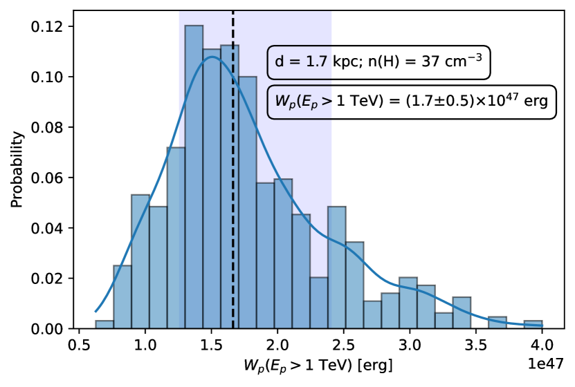
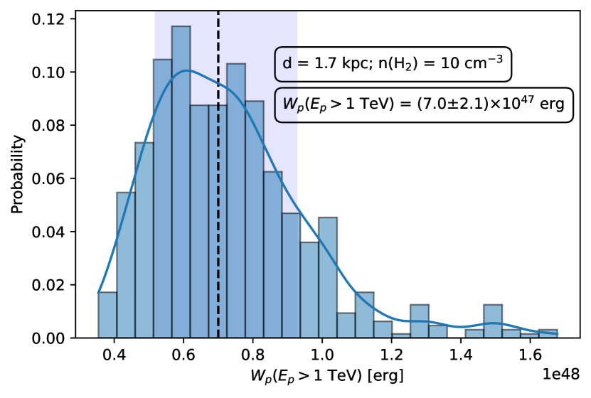
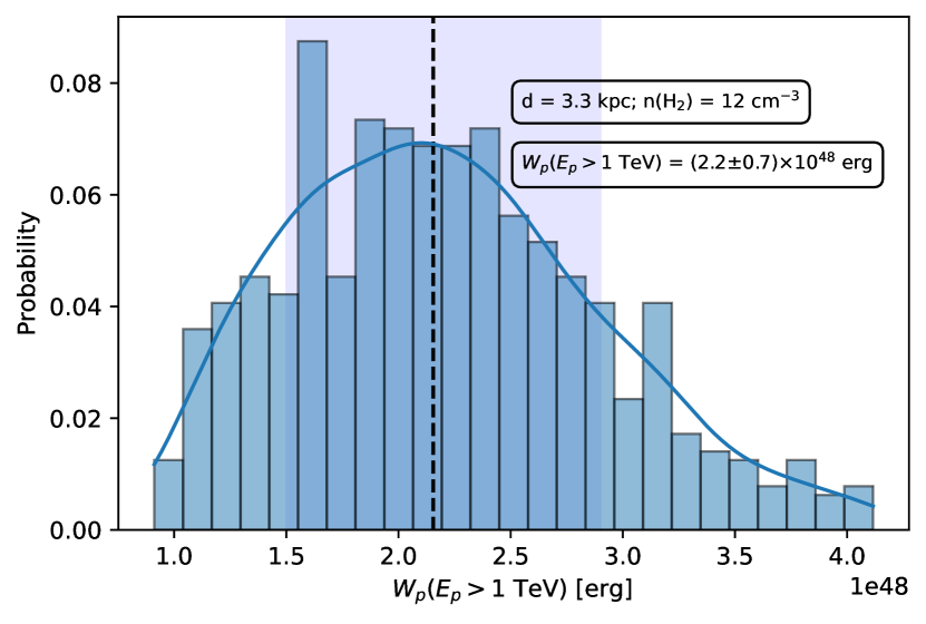
Figure 9: Computed Hadronic model using Naima for [FKT-MC]2022, considering LHAASO parameters (Cao et al., 2021a), a distance of 1.7 kpc, and optically thin gas for a) density of nucleons n(H) = 37 cm^-3, and b) n(H₂) = 10 cm^-3 (this work). c) The same for the [MML2017]4607 molecular cloud, but considering a distance of 3.3 kpc, and optically thick gas with n(H₂) = 12 cm^-3 from Miville-Deschenes, Murray, & Lee (2017).

The first spectral energy distribution (SED) of J2108 was presented by Cao et al. (2021b). Nevertheless, this SED does not include RXJ2107.3$+$5202 and the NVSS emission. In Fig. 8 we show this SED with these two emissions. The SED was calculated using the models of Zabalza (2016) in Naima software. A similar complementary SED is presented by Kar & Gupta (2022). At high energies, it is complicated to distinguish between the leptonic and hadronic nature of the emission (see § 2.2 and Cao et al. 2021b), although the leptonic nature seems to be favoured at lower energies.

The hadronic and leptonic modeling considers a power law spectrum with an exponential cutoff and fixed spectral indexes of 2.0 and 2.2, respectively. In the leptonic modeling we adopt an energy cutoff of 200 TeV and a magnetic field strength of 3 $\mu$G (Cao et al., 2021b). For IC scattering, we include CMB and IR seed photon fields with temperatures of 2.72 and 20.0 K, and energy densities of 0.26 and 0.3 eV cm^-3, respectively (e.g. Hinton and Hofmann, 2009; Vernetto & Lipari, 2016). Considering a distance of 1.7 kpc, we obtain a total energy of electrons with energy above 1 GeV of 2.2 $\pm$ 0.4 $\times 10^{46}$ erg. Nevertheless, no clear source for the leptonic emission nor extended X-ray emission in the vicinity (neither in the FOV nor in Kron 82) has been observed or reported.

Regarding this fact and the presence of two molecular clouds (MML and [FKT-MC]2022) as candidates for the generation of the sub-PeV emission, we favour the scenario of a hadronic origin: gamma rays generated by the decay of neutral pions due to the interaction between accelerated protons and molecular clouds. Here, the pion decay model in Zabalza (2016) is based on Kelner, Aharonian, & Bugayov (2006); Kamae et al. (2006) and implemented by Kafexhiu et al. (2014). We used a distance of 3.3 kpc for MML (Cao et al., 2021b) and 1.7 kpc for [FKT-MC]2022, considering ROIs of 0.5^∘ and 1.1^∘, respectively. We use a nucleon number density of 30 cm^-3 (estimated by Cao et al., 2021b) for MML and 37 cm^-3 for [FKT-MC]2022, and calculate the total proton energy as follows:

$$\Bigg{[}\frac{\rm E_{P}}{\rm erg}\Bigg{]}=9.0\pm 3.0\times 10^{47}\Bigg{[}\rm\frac{n(H)}{30~{}cm^{-3}}\Bigg{]}^{-1}\Bigg{[}\rm\frac{D}{3.3~{}kpc}\Bigg{]}^{2}\quad\rm{for\ MML},$$ (10)

and

$$\Bigg{[}\rm\frac{E_{P}}{erg}\Bigg{]}=1.7\pm 0.5\times 10^{47}\Bigg{[}\rm\frac{n(H)}{37~{}cm^{-3}}\Bigg{]}^{-1}\Bigg{[}\rm\frac{D}{1.7~{}kpc}\Bigg{]}^{2}\\ \rm{for\ FKT}.$$ (11)

In Tab. 6, we show the results of several hadronic models (via neutral pion decay process) by using Naima software, considering different parameters for [FKT-MC]2022 and MML. In Fig. 9 we show the energy distribution of the proton population (with energy above 1 TeV) of three of the hadronic models: [FKT-MC]2022 with a proton density of 37 cm^-3, [FKT-MC]2022 with an optically thin H₂ density of 10 cm^-3, and MML with an optically thick H₂ density of 12 cm^-3 (Miville-Deschenes, Murray, & Lee, 2017). Comparing these energy distributions, the W_p (7$\pm$2$\times$10⁴⁷ erg) of [FKT-MC]2022 (optically thin gas with H₂ density of 10 cm^-3) is close to that for MML of 2.2$\pm$0.7$\times$10⁴⁸ erg (optically thick gas with H₂ density = 12 cm^-3). The latter is consistent with the W_p = 2.0$\times$10⁴⁸ erg reported in Cao et al. (2021b), which was calculated using the Naima software with a distance of 3.3 kpc, and optically thick gas approximation with n(H) = 2n(H₂) = 30 cm^-3.

On the other hand, for [FKT-MC]2022 at 100 TeV and assuming no leptonic contribution, we obtain a flux of E² $\frac{dN}{dE}$ $\sim$ 2 $\times$ 10^-13 erg cm^-2 s^-1 from the hadronic contribution of Fig. 8. The latter corresponds to a differential flux of N${}_{\gamma}^{\rm had}$ = 1.25 $\times$ 10^-17 photons TeV^-1 cm^-2 s^-1. This value corresponds to the N${}_{P}({\rm CR})$ = 1.04 $\times$ 10^-29 TeV^-1 in Eq. 2

[FKT-MC]2022 (see Eq.  11) reproduces an observed differential flux of $\sim$ 10^-17 photons TeV^-1 cm^-2 s^-1 (Fig. 8) assuming an optically thin nucleon density of n(H) = 37 cm^-3. This flux corresponds to an E_P ($\sim 1.7\times 10^{47}$ erg), which is slightly less than the required energy for MML ($\sim 9.0\times 10^{47}$ erg; optically thick gas). In addition, a lower required energy of $E_{\rm P}=$ 6.7 $\pm$ 2.3 $\times 10^{46}$ ergs is obtained [FKT-MC]2022, if a distance of 1.2 kpc (obtained with the rotation curve of Reid et al. 2014) and a nucleon density of 52 cm^-3 are considered. Finally, if we project the size of [FKT-MC]2022 to the distance of MML (3.3 kpc) or if we project MML to a distance of [FKT-MC]2022, the size of the clouds matches accordingly (see Tab. 5).

The energies of both molecular clouds are much lower than the energy of a single SN ($\sim$ 10⁵¹ erg). Therefore, an ancient unidentified SNR could be the PeVatron(e.g Kar & Gupta, 2022, and references therein). Ultimately, we favour the presence of a molecular cloud, MML or [FKT-MC]2022, as a place to produce the emission observed by LHAASO in J2108. High-resolution radio observations, including denser gas tracers, are needed to clarify the scenery.

6 Conclusions

We present low-resolution ^12,13CO(2$\rightarrow$1) observations made with the 1.85-m radio-telescope at Osaka Prefecture University to detect a molecular counterpart to the PeVatron associated with LHAASO J2108+5157 in the OB7 molecular cloud at Cygnus. We discuss the methodology to obtain the observed flux of gamma-ray emission by determining an appropriate density of nucleons, including HI and H₂ (through CO observations) emissions:

• In addition to MML[2017]4607, we propose molecular cloud [FKT-MC]2022 as another candidate to produce the observed emission for LHAASO J2108+5157, favouring the hadronic emission because neither a source nor data support leptonic emission.

• $[$FKT-MC$]$2022 is situated at a distance of 1.7 $\pm$ 0.6 kpc. It is $\sim$ 1.1^∘ in size and has nucleon densities (HI + H₂) of $\sim$ 80 and 37 cm^-3 for ¹²CO (optically thick) and ¹³CO (optically thin) emission respectively. These values correspond to M(HI +H₂) of $\sim$ 4$\times$10⁴ M_⊙ and 2$\times$10⁴ M_⊙ respectively. We computed a total required energy of protons of W${}_{p}\sim 1.7\times 10^{47}$ erg to reproduce the gamma-ray emission observed by LHAASO.

• The ^12,13CO(2$\rightarrow$1) observations of Kronberger 82 reveal a clump morphology with a V_LSR $\sim$ –7 km s^-1 and a size of 0.1^∘. For optically thin gas at a distance between 1.63 and 2.30 kpc, the n(HI+2H₂) or n(H) is between 1.7 and 2.5 $\times$ 10³ cm^-3 and M(HI +H₂) is between 0.4 and 1.7 $\times$ 10³ M_⊙. These values are consistent with the optically thick gas and with other molecular observations, confirming Kronberger 82 as a star-forming region rich in molecular species

• By modelling its hadronic gamma-ray emission, Kronberger 82 uses less energy (W${}_{p}\sim 2.6-7.0\times 10^{45}$ erg) to produce the observed (sub)PeV gamma-ray emission in LHAASO J2108+5157 than [FKT-MC]2022 and MML[2017]4607. Nevertheless, due to its angular separation from J2108+5157, it is not a strong candidate to be the gamma-ray source.
  

Conflict of Interest

The authors state that have no conflict of interest directly relevant to the content of this article

This work was (partially) supported by the Inter-University Research Program of Institute for Cosmic Ray Research (ICRR), the University of Tokyo. IT–J acknowledges support from Consejo Nacional de Ciencia y Tecnología (CONACyT), México; grant 754851. We are grateful for the computational resources and technical support offered by the Data Analysis and Supercomputing Center (CADS) through the Leo-Atrox supercomputer of the Universidad de Guadalajara. EdelaF thanks colegio departamental, departamento de Física, and respective authorities of the Centro Universitario de Ciencias Exactas e Ingenierías (CUCEI), Universidad de Guadalajara, for authorization and permissions to perform the academic stays.

Chapter 1 Determination of column densities and n(H)

First, we compare the distribution of HI with the ^12,13CO gas to reliably clarify the position of the associated molecular cloud. Then we obtain the spectra and calculate the physical parameters in a standard way.

Assuming optically thin emission, the column density (N) using HI is computed as (Dickey & Lockman, 1990):

$$\left[\frac{N({\rm HI})}{\rm cm^{-2}}\right]=1.823\times 10^{18}\left[\frac{\int T_{\rm MB}^{HI}dv}{\rm K\ km\ s^{-1}}\right],$$ (1.1)

where $T_{\rm MB}^{HI}$ is the averaged brightness temperature of the main beam (MB) resulting from a Gaussian fit of the spectrum of HI emission.

Under LTE conditions and assuming ¹²CO optically thick gas the excitation temperature $T_{\rm ex}$ is:

$$T_{\rm ex}=\frac{T_{0}}{\ln\left(1+\frac{T_{0}}{T_{\rm MB}^{12,p}+T_{0}/\left(\exp(T_{0}/T_{\rm CMB})-1\right)}\right)},$$ (1.2)

where $T_{\rm MB}^{12,p}$ is the main beam averaged peak temperature of the ¹²CO emission, T_CMB = 2.725 K is the temperature of the cosmic microwave background (CMB) and $T_{0}=h\nu/k$ is the characteristic temperature of the ^12,13CO (J=2$\rightarrow$1) at a rest frequency of $\nu^{12}_{\rm CO}=$ 230.538 and $\nu^{13}_{\rm CO}=$ 220.398 GHz, respectively. The optical depth $\tau^{13}_{\rm CO}$ of the ¹³CO gas is determined assuming an optically thin emission and using (Rohlfs, 2004):

$$\tau^{13}_{\rm CO}=-\ln\Bigg{[}1-\frac{J_{\nu}^{12}(T_{\rm ex})-J_{\nu}^{12}(T_{\rm CMB})}{J_{\nu}^{13}(T_{\rm ex})-J_{\nu}^{13}(T_{\rm CMB})}\frac{T_{\rm MB}^{13,p}}{T_{\rm MB}^{12,p}}\Bigg{]},$$ (1.3)

where $T_{\rm MB}^{13,p}$ is the main beam averaged peak temperature of the ¹³CO emission and,

$$J_{\nu}(T)=\frac{h\nu/k}{e^{h\nu/kT}-1},$$ (1.4)

is the intensity in units of temperature related with the CMB and the excitation temperature for the ^12,13CO(J=2$\rightarrow$1) emission.

From Scoville et al. (1986) and Palau et al. (2007) we derived an expression to calculate the column density of ¹³CO from a rotational transition $J\to J-1$ as

$$\begin{split}\left[\frac{N(\rm^{13}CO)}{\rm cm^{-2}}\right]&=4.70\times 10^{13}\frac{T_{\rm ex}}{J^{2}}\exp\left(\frac{2.64\ J(J+1)}{T_{\rm ex}}\right)\\ &\times\frac{\tau^{13}_{\rm CO}}{1-e^{-\tau^{13}_{\rm CO}}}\left[\frac{\int T_{\rm MB}^{13}(v)dv}{\rm K\ km\ s^{-1}}\right],\end{split}$$ (1.5)

where the integrated brightness temperature of the main beam for the ¹³CO emission, $\int T^{13}_{\rm MB}(v)dv$, is obtained from the Gaussian fit for the respective velocity component of the ¹³CO spectrum. Taking a standard value for the isotopic abundance ratio of $\rm{}^{12}CO/^{13}CO\approx 60$ for the ISM (Langer et al., 1993), we estimate the optical depth of ¹²CO as $\tau^{12}_{\rm CO}$= 60$\tau^{13}_{\rm CO}$. Similarly, the column density of ¹²CO can then be calculated with (Palau et al., 2007):

$$\begin{split}\left[\frac{N(\rm^{12}CO)}{\rm cm^{-2}}\right]&=4.33\times 10^{13}\frac{T_{\rm ex}}{J^{2}}\exp\left(\frac{2.77\ J(J+1)}{T_{\rm ex}}\right)\\ &\times\frac{\tau^{12}_{\rm CO}}{1-e^{-\tau^{12}_{\rm CO}}}\left[\frac{\int T_{\rm MB}^{12}(v)dv}{\rm K\ km\ s^{-1}}\right].\end{split}$$ (1.6)

where $\int T^{12}_{\rm MB}(v)dv$ is the integrated brightness temperature of the main beam for the ¹²CO emission. Using an abundance ratio of $[\rm H_{2}/^{13}CO]=10^{5}$ (Dickman, 1978; Pineda et al., 2008), the column density of H₂ (via the ¹³CO emission) can be estimated by

$$N(\rm{H_{2}})=5\times 10^{5}\ N(^{13}{\rm CO})$$ (1.7)

Moreover, several studies (e.g Bolatto et. al, 2013) find a “¹²CO-to-H₂” conversion factor with a Galactic mean of $X_{\rm CO}=$ 2.0 $\times 10^{20}$ cm^-2 (K km s^-1)^-1 with 30% uncertainty within the Milky Way disk. Then, the H₂ column density (via the ¹²CO emission) can be estimated as:

$$N({\rm H_{2}})=X_{\rm CO}\int T_{\rm MB}^{12}(v)dv$$ (1.8)

Finally, the total proton column density N(H) is calculated using Eq. 4.

Chapter 2 IRAS 21046+5110 and Kronberger 82

B.1 IRAS 21046+5110

IRAS 21046 is a star-forming region with more than 200 massive protostellar candidates in 54 embedded clusters at a distance of $\sim$ 600 pc (Kumar, Keto, & Clerkin, 2006). These authors present a complete and detailed NIR study confirming that the clusters and their properties have more to do with the formation process than with evolution. Considering its stellar content mass, M_stellar, of 17 M_⊙ (Kumar, Keto, & Clerkin, 2006), the clear but fainter OPU ¹³CO(J=2$\to$1) emission compared to Kron 82 (integrated flux ratio $\sim$ 0.3; see Fig. 3), its farthest distance from J2021 compared to Kron 82 ($\sim$ 0.7^∘ vs. $\sim$ 0.4^∘), and the fact that its nature is not comparable to the Cygnus OB2, we do not support it as a producer of the sub-PeV emission observed by LHAASO. Furthermore, it was not considered in the inspection of Cao et al. (2021b).

B.2 Kronberger 82

Kron 82 is a poorly studied star-forming region. A visual inspection of IR using 2MASS (images not shown), IRAC, WISE, and NVSS emission (see lower panels in Fig. 2) suggests that Kron 82 has the classic IR morphology observed in star-forming regions, including ultra-compact HII regions with extended emission and OB stars covered by arcminute-sized RC emission (e.g de la Fuente, et al., 2020a, b; Churchwell et al., 2007, and references therein). The latter implies that ionised gas coexists with star clusters (2.12 $\mu$m, 3.6 $\mu$m, 4.5 $\mu$m and RC at 20 cm; in agreement with the corresponding WISE emission), with associated dust traced at WISE 22 $\mu$m (no IRAC data at 5.8, 8.0 and 24 $\mu$m). In this context, the remarkable HII region IRAS 21078+5211 (distance of $\sim$ 1.6 kpc; Moscadelli et al. 2021 and references therein), the star-forming region IRAS 21078+5209 (distance of $\sim$ 1.5 kpc; see Gieser et al. (2021) and references therein), and the star cluster DSH J2109.5+5223 (Kronberger et al., 2006) are located in the interior of the Kron 82 region. Nevertheless, a literature search for massive and WR stars in the vicinity, and a quick 2MASS photometry shows that Kron 82 resembles more IRAS 21046+5110 than Cygnus OB2: ruled by YSOs and no WR detected. A more detailed study of the stellar content in IR is needed to determine the nature of Kron 82 as a star cluster (formation dominated by YSOs like IRAS 21046, or evolution dominated like Cygnus OB2 with intense stellar winds).

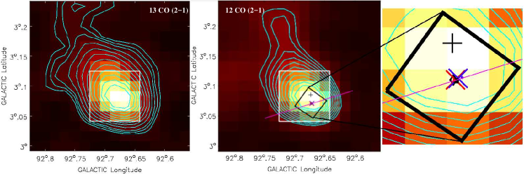
Figure 10: Same as the bottom left of Fig. 2, but for the OPU ^12,13CO(J=2$\rightarrow$1) emission of Kron 82 (colours and contours). The selected region of 0.1^∘ that was used to extract the spectrum in Fig. 11 is shown as a square in the leftmost panel of the Figure. In the middle panel, the rotated square, which indicates the direction of the equatorial coordinates, shows the region studied at higher angular–resolution by Moscadelli et al. (2021); see their Fig. 2. The peak position of the IRAM 30 m data is shown as a diamond mark right at the centre of the rotated square. In the same panel the cross corresponds to the tip of the protrusion of the emission observed their Fig. 2. The blue and red ”x” marks indicate the position of the blue-and red–shifted, respectively, SW lobes originating from source 1 (see their Figs 1 and 5). The line shows the projection of these lobes when transferred to larger scales. The size of the beam is 0.045${}^{\circ}\times$0.045^∘..

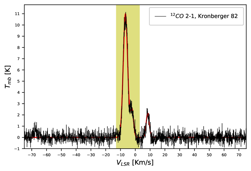
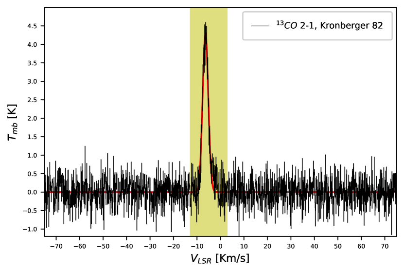
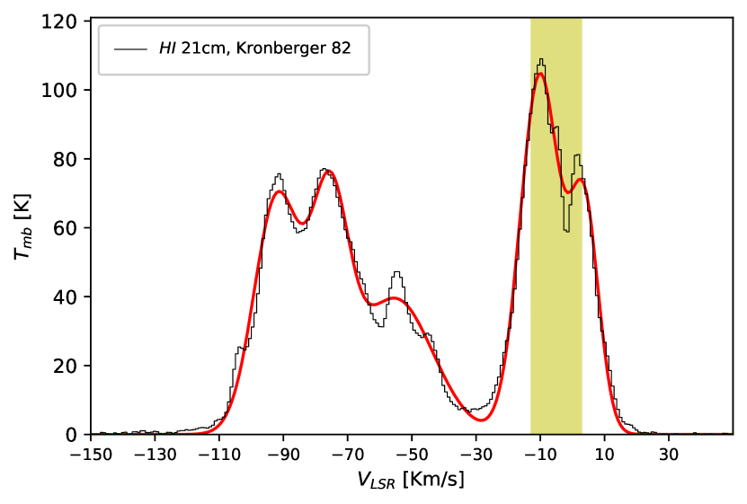
Figure 11: Same as Fig. 7 but for Kronberger 82 (see Fig. 2). The weak component at $\sim$ 7 km s^-1 corresponds to COB-7 gas in the vicinity.

In Fig. 10 we show the low-resolution ^12,13CO(J=2$\to$1) emission maps of the OPU around Kron 82 (cf. Fig. 1 down ). The white square represents the region of $\approx$ 0.1 deg around the brightest emission where the spectra were extracted. The averaged spectra for ^12,13CO(J=2$\to$1) and HI emissions are shown in Fig. 11. The fitting parameters are shown in Tab. 7. The black square, the crosses and the plus sign refer to objects studied by Moscadelli et al. (2021).

¹²CO (J=2$\to$1) and ¹³CO (J=2$\to$1) spectra show the brightest principal component in a –13 $\gtrsim$ V_LSR $\gtrsim$ 3 km s^-1 range, centered at V${}_{\rm LSR}\sim$ –6.6 km s^-1 (see Tab. 7). This value agrees with the systemic velocity of $\sim$ 6.1 km s^-1 reported by Moscadelli et al. (2021). Besides the main line in the ¹²CO(J=2$\to$1) spectrum, we discover a weak wing component at $\sim$ –2.2 km s^-1. This component is probably related to the main velocity component of the CO gas in the COB7-MC region. On the other hand, the ¹²CO(J=2$\to$1) spectrum shows another weak component at V_LSR of 8.41 km s^-1 with an observed frequency of 230.5315 GHz and a signal-to-noise ratio $\sim$ 6. We believe this line is related to CO molecular gas in COB7–MC, but high-resolution observations are needed to clarify its nature.

To estimate the physical parameters, we consider emission in the range V${}_{\rm LSR}=$ -13 to 3 km s^-1 (see Fig. 11), which includes both the main and wing components of the ¹²CO(J=2$\to$1) spectrum. The fitted parameters in this range are shown in Tab. 8.

We follow the same methodology described in section 5.1.2 for the molecular cloud and use the peak brightness of the principal component to estimate the average excitation temperature using Eq. 1.2 and the corresponding optical depth using Eq. 1.3. We obtain an average of $T_{\rm ex}\sim$ 16 K within this region. The optical depth $\tau^{12}_{CO}$ is then estimated from $\tau^{13}_{CO}$. Next, the column densities of ¹³CO and ¹²CO are calculated using Eqs. 1.5 and 1.6, respectively. The H₂ column density is estimated using the equations  5 and 1.6. The results are shown in Tab. 9. Finally, the number density of H₂ and H (H₂+ HI) is calculated using the distance to Kron 82 $\approx$ 1.63 kpc (Moscadelli et al., 2021; Xu et al., 2013) and the Eq. 7, which is shown in Tab. 10. The physical parameters agree with those of Moscadelli et al. (2021).

On the other hand, using the rotation curve of (Brand & Blitz, 1993), we obtain a far kinematic distance of 2.3$\pm$ 0.5 kpc. The parameters calculated at this distance are also shown in Tab. 10 for comparison with those calculated at 1.63 kpc. The estimated physical parameters are similar at both distances. Thus, in a distance range between 1.63 and 2.30 kpc, Kron 82 is a molecular clump with a size of $\sim$ 0.1^∘; a nucleon density (H₂+ HI) of about 10³ cm^-3 and an M(H₂+ HI) of 10³ M_⊙. The estimated H₂ number densities, H₂ total mass, and the viarl mass are shown in Tab. 11. We show the results for the computed hadronic model in Fig. 12 and Tab. 12, taking into consideration these physical parameters and utilizing the same models derived by Naima as stated in  § 5.1.3. We calculated proton energies of 2.6 $\times$ 10⁴⁵ and 7.0 $\times$ 10⁴⁵ ergs for distances of 1.63 and 2.3 kpc, respectively.

Comparing these values to those of MML and [FKT-MC]2022 (9.0$\times$10⁴⁷ ergs and 1.6$\times$10⁴⁷ ergs; see Fig. 9), Kron 82 requires significantly less cosmic-ray energy (proton) to replicate the emission of J2108, regardless of whether it was caused by a supernova explosion or massive stellar winds. These energies are $\sim$ 10⁵¹ erg for supernova explosions and $\sim$ 10⁵² erg for stellar winds from star clusters similar to Cygnus OB2 (e.g. Lozinskaya et al., 2002, and references therein). Even if Kron 82 appears to have a stellar component more similar to IRAS 21046+5110 than Cygnus OB2, it is possible for molecular gas to produce the LHAASO-measured energy for J2108. Nonetheless, due to its 0.4^∘ radius separation from J2108, outside its (sub-PeV emission) upper limit radial extension ($\sim$ 0.35^∘; Cao et al., 2021b), this scenery is not favorable.

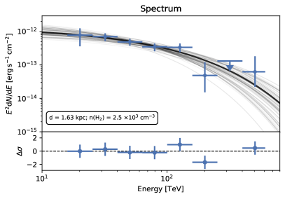
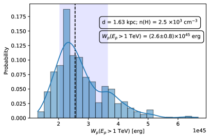
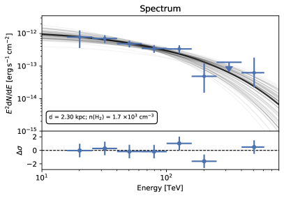
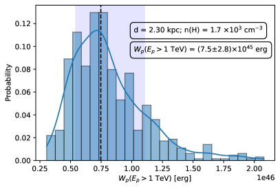
Figure 12: Same as Fig. 9, but for Kronberger 82. The hadronic model was calculated for the range of a) 1.63 kpc and b) 2.30 kpc. We use the respective nucleon density given in Tab. 10 and a cutoff of 600 TeV (see Tab. 12). The total proton energy of $\sim$ 10⁴⁵ ergs required to reproduce the flux observed by LHAASO (blue points) is lower than those of [FKT-MC]2022 and MML (W_p $\sim$ 10⁴⁷ ergs), so we cannot discard Kron 82 as a candidate for J2108 sub-PeV emission.

Table 7: Parameters of the adjusted Gaussian fits of the emissions of ¹²CO(J=2$\rightarrow$1) and ¹³CO(J=2$\rightarrow$1) around Kron 82. The main beam (MB) averaged peak temperature ($T^{p}_{\rm MB}$) uncertainties are only due to rms noise. Velocity channel resolutions are used to show the LSR velocity (V_LSR) and FWHM ($\Delta V$) uncertainties.

Line	Diameter	VLSR	$\Delta V$	$T_{\rm MB}^{\rm peak}$	$\int T_{\rm MB}dV$
	[deg]	$\rm km\ s^{-1}$	$\rm km\ s^{-1}$	[K]	[K km s-1]
12CO 2-1 main	0.10 $\pm$ 0.01	-6.64 $\pm$ 0.08	3.511 $\pm$ 0.08	11.00 $\pm$ 0.40	41.10 $\pm$ 0.56
12CO 2-1 wing	0.10 $\pm$ 0.01	-2.24 $\pm$ 0.08	2.48 $\pm$ 0.14	2.46 $\pm$ 0.40	6.48 $\pm$ 0.45
12CO 2-1 weak	0.10 $\pm$ 0.01	8.41 $\pm$ 0.08	2.44 $\pm$ 0.13	2.16 $\pm$ 0.40	5.60 $\pm$ 0.40
13CO 2-1	0.10 $\pm$ 0.01	-6.39 $\pm$ 0.08	2.83 $\pm$ 0.08	4.30 $\pm$ 0.40	12.95 $\pm$ 0.41

Table 8: Values used for the column density analysis (Kronberger 82).

Species	Diameter	$T_{\rm MB}^{\rm peak}$	$\int T_{\rm MB}dV$	$T_{\rm ex}$	$\tau$
	[deg]	[K]	[K km s-1]	[K]
12CO 2-1 main + wing	0.10 $\pm$ 0.02	11.00 $\pm$ 0.40	47.58 $\pm$ 0.72	16.1 $\pm$ 0.4	29.2 $\pm$ 3.4
13CO 2-1	0.10 $\pm$ 0.02	4.30 $\pm$ 0.40	12.95 $\pm$ 0.41	16.1 $\pm$ 0.4	0.5 $\pm$ 0.1
HI	0.10 $\pm$ 0.02	–	1379.3 $\pm$ 304.3	–	–

Table 9: Estimated column (N) and number (n) densities of HI, ¹²CO, ¹³CO, and $\rm H_{2}$ for Kronberger 82. The 12 and 13 labels correspond to the respective CO emission used in the calculations.

Diameter	$N(\rm^{13}CO)$	$N(\rm^{12}CO)$	$N(\rm HI)$	$N^{\rm{}^{12}CO}(\rm H_{2})$	$N^{\rm{}^{13}CO}(\rm H_{2})$	$n^{{}^{12}CO}(\rm H_{2})$	$n^{{}^{13}CO}(\rm H_{2})$
deg	[$10^{15}$ cm-2]	[$10^{17}$ cm-2]	[$10^{21}$ cm-2]	[$10^{21}$ cm-2]	[$10^{21}$cm-2]	[$10^{3}$cm-3]	[$10^{3}$cm-3]
0.10 $\pm$ 0.01	8.3 $\pm$ 0.3	6.8 $\pm$ 0.8	2.5 $\pm$ 0.5	9.5 $\pm$ 2.8	4.1 $\pm$ 1.2	1.1 $\pm$ 0.3	0.5 $\pm$ 0.1

Table 10: Column (N) and number (n) densities of nucleons for Kronberger 82.

Diameter	Distance	$N^{12}(\rm H)$	$N^{13}(\rm H)$	$n^{12}(\rm H)$	$n^{13}(\rm H)$
$[\rm deg]$	[kpc]	[$10^{22}\rm cm^{-2}$]	[$10^{22}\rm cm^{-2}$]	[$10^{3}\rm cm^{-3}$]	[$10^{3}\rm cm^{-3}$]
0.10 $\pm$ 0.01	1.63 $\pm$ 0.05	1.1 $\pm$ 0.3	2.2 $\pm$ 0.6	2.5 $\pm$ 0.7	1.2 $\pm$ 0.3
0.10 $\pm$ 0.01	2.30 $\pm$ 0.50	1.1 $\pm$ 0.3	2.2 $\pm$ 0.6	1.7 $\pm$ 0.6	0.9 $\pm$ 0.3

Table 11: Parameters of the molecular emission for Kronberger 82

Source	VLSR	$D$	Distance	$M_{\rm vir}({\rm H_{2}})$	$M({\rm H_{2}})$	$M(\rm HI+H_{2})$
	[$\rm km\ s^{-1}$]	[deg]	[kpc]	[$10^{4}M_{\odot}$]	[$10^{3}M_{\odot}$]	[$10^{3}M_{\odot}$]
Kronberger 82 (13CO)	-6.6 $\pm$ 0.1	0.10 $\pm$ 0.01	1.63 $\pm$ 0.05	2.4 $\pm$ 0.1	0.4 $\pm$ 0.1	0.5 $\pm$ 0.1
Kronberger 82 (12CO)	-6.6 $\pm$ 0.1	0.12 $\pm$ 0.01	1.63 $\pm$ 0.05	3.7 $\pm$ 0.1	1.5 $\pm$ 0.5	1.7 $\pm$ 0.5
Kronberger 82 (13CO)	-6.6 $\pm$ 0.1	0.10 $\pm$ 0.01	2.33 $\pm$ 0.51	2.4 $\pm$ 0.1	0.3 $\pm$ 0.1	0.4 $\pm$ 0.1
Kronberger 82 (12CO)	-6.6 $\pm$ 0.1	0.12 $\pm$ 0.01	2.33 $\pm$ 0.51	3.7 $\pm$ 0.1	1.1 $\pm$ 0.4	1.2 $\pm$ 0.4

Table 12: Naima Results for Kronberger 82

	Distance	n(H)	ROI	$W_{p}$	Cutoff	Obtained
	[kpc]	[cm-3]	[deg]	[$10^{45}$erg]	[TeV]	from
Kron 82 2022	1.63	2.5 $\times$ 103	0.1	2.6${}_{-0.5}^{+1.1}$	$600\pm 300$	13CO(J=2$\rightarrow$1)
Kron 82 2022	2.30	1.7 $\times$ 103	0.1	7.0${}_{-2.0}^{+4.0}$	$600_{-200}^{+400}$	13CO(J=2$\rightarrow$1)

References

- Abeysekara et al. (2020) Abeysekara, A. U., et al. 2020, PRL, 124, 021102
- Abeysekara et al. (2021) Abeysekara, A.U, et al. 2021, Nat. Astron., 5, 465
- Abdollahi et al. (2020) Abdollahi, S., Acero, F., Ackermann, M., et al. 2020, ApJS, 247, 33
- Ackermann et al. (2011) Ackermann, M., et al. 2011, Science, 334, 1103
- Ade et al. (2011) Ade, P. A. R., Aghanim, N., Arnaud, M., Ashdown, M., et al. 2011, A&A, 536, 19
- Aharonian et al. (2019) Aharonian, F., et al., 2019, Nat. Astron., 3, 561
- Albert et al. (2021) Albert, A., et al. 2020, ApJ, 911, 143
- Albert et al. (2020a) Albert, A., et al. 2020, ApJ, 896, L29
- Albert et al. (2020b) Albert, A., et al. 2020, ApJ, 905, 1
- Albert et al. (2007) Albert, J., et al. 2007, ApJ, 664L, 87
- Ambrocio-Cruz, Rosado, & de La Fuente, E. (2006) Ambrocio-Cruz, P., Rosado, M., & de La Fuente, E. 2006, RMxAA, 42, 241
- Amenomori et al. (2019) Amenomori, M., et al. 2019, PRL, 123, 051101 (2019)
- Amenomori et al. (2021a) Amenomori, M., et al. 2021a, Nat. Astron., 5, 460
- Amenomori et al. (2021b) Amenomori, M., et al. 2021b, PRL, 126, 141101
- Amenomori et al. (2021c) Amenomori, M., et al. 2021c, PRL, 127, 031102
- Bolatto et. al (2013) Bolatto A. D., Wolfire M., Leroy A. K., 2013, ARA& A, 51, 207
- Brand & Blitz (1993) Brand J., Blitz L., 1993, A&A, 275, 67
- Cao et al. (2021a) Cao, Z., et al. 2021a, Nature, 594, 33
- Cao et al. (2021b) Cao, Z., et al. 2021b, ApJ, 919, L22
- Churchwell et al. (2007) Churchwell, E., Watson, D. F., Povich, M. S., Taylor, M. G. 2007, ApJ, 670, 428
- Condon et al. (1998) Condon, J. J., et al. 1985, AJ, 115, 1693
- Dame, Hartmann, & Thaddeus (2001) Dame, T. M., Hartmann, D., & Thaddeus, P. 2001, ApJ, 547, 792
- de la Fuente, et al. (2020a) de la Fuente, E., Porras, A., Trinidad, M. A., Kurtz, S. E. 2020a, MNRAS, 492, 895
- de la Fuente, et al. (2020b) de la Fuente, E., Tafoya, D., Trinidad, M. A., Porras, A. 2020b, MNRAS, 497, 4436
- Dickey & Lockman (1990) Dickey, J. M., and Lockman, F. J. 1990, ARA&A, 28, 215
- Dickman (1978) Dickman RL. 1978. Ap. J. Suppl. 37:407–27
- Dobashi et al. (1994) Dobashi, K., Bernard, J.-Ph., Yonekura, Y., & Fukui, Y. 1994, ApJS, 95, 419
- Dobashi, Bernard, & Fukui (1996) Dobashi, K., Bernard, J.-Ph., & Fukui, Y. 1996, ApJ, 466, 282
- Dobashi et al. (2018) Dobashi, K., Shimoikura, T., Endo, N., Takagi, C., et al. 2019, PASJ, 71, S11
- Dobashi et al. (2014) Dobashi, K., Matsumoto, T., Shimoikura, T., Saito, H., et al. 2014, ApJ, 797, 58
- Erging et al. (2017) Ergin, T., Sezer, A., Sano, H., & Yamazaki, R. 2017, ApJ, 842, 22
- Fukui et al. (2021) Fukui, Y., Sano, H., Yamane, Y., et al. 2021, ApJ, 915, 84
- Fukui et al. (2012) Fukui, Y., Sano, H., Sato, J., et al. 2012, ApJ, 746, 82
- Garay and Lizano (1999) Garay, G. and Lizano, S., 1999, PASP, 111, 1049
- Gieser et al. (2021) Gieser, C., Beuther, H., Semenov, D., Ahmadi, A., 2021, A&A, 648, A66
- Humphreys (1978) Humphreys, R. M. 1978, ApJS, 38, 309
- Hinton and Hofmann (2009) Hinton, J. A., and Hofmann, W. 2009, ARA&A, 47, 523
- Jackson et. al (2002) Jackson, J. M., Bania, T. M., Simon, R., et al. 2002, ApJ, 566 L81
- Jiang et. al (2010) Jiang, B., Chen, Y., Wang, J., Su, Y., et al. 2010, ApJ, 712, 1147
- Kafexhiu et al. (2014) Kafexhiu, E., Aharonian, F., Taylor, A.M., & Vila, G.S. 2006, Phys. Rev. D, 90, 123014
- Kamae et al. (2006) Kamae, T., Karlsson, N., Mizuno, T., Abe, T., & Koi, T. 2006, ApJ, 647, 692
- Kar & Gupta (2022) Kar, A., & Gupta, N. 2022, ApJ, 926, 110
- Karpova et al. (2016) Karpova, A., Shternin, P., Zyuzin, D.,Danilenko, A., et al. 2016, MNRAS, 462, 3845
- Kelner, Aharonian, & Bugayov (2006) Kelner, S. R., Aharonian, F. A., and Bugayov, V. V. 2006, Phys. Rev. D, 74, 034018
- Kronberger et al. (2006) Kronberger, M., Teutsch, P., Alessi, B., et al. 2006, A&A, 447, 921
- Kumar, Keto, & Clerkin (2006) Kumar, M. S. N., Keto, E., & Clerkin, E. 2006, A&A, 449, 1033
- Langer et al. (1993) Langer W. D. and Penzias A. A. 1993, ApJ, 408, 539-547.
- Lozinskaya et al. (2002) Lozinskaya, T. A., Pravdikova, V. V., and Finoguenov, A. V. 2002, Astron. Lett. 28, 223-236
- Miville-Deschenes, Murray, & Lee (2017) Miville-Deschenes, M.-A., Murray, N., & Lee, E. J. 2017, ApJ, 834, 57
- Motch et al. (1997) Motch, C., Guillout, P., Haberl, F., Pakull, M. W., et al. 2017, A&AS, 122, 201
- Moscadelli et al. (2021) Moscadelli, L., Beuther, H., Ahmadi, A., Gieser, C. 2021, A&A, 647, A114
- Nishimura et al. (2020) Nishimura, A., Tokuda, K., Kimura, K., et al. 2020, Proceedings of the SPIE, 11445, 114457F1-114457F13. doi:10.1117/12.2560955
- Nishimura et al. (2015) Nishimura, A., Tokuda, K., Kimura, K., et al. 2015, ApJS, 216, 18. doi:10.1088/0067-0049/216/1/18
- Palau et al. (2007) Palau, A., et al. 2007, A&A, 474, 911
- Pineda et al. (2008) Pineda JE, Caselli P, Goodman A. A. 2008. ApJ. 679:481–96
- Onishi et al. (2013) Onishi, T., Nishimura, A., Ota, Y., et al. 2013, PASJ, 65, 78. doi:10.1093/pasj/65.4.78
- Reid et al. (2014) Reid M. J., et al., 2014, ApJ, 783, 130
- Reipurth & Schneider (2008) Reipurth B., & Schnider, N. 2008, in Handbook of Star Forming Regions Vol. I Astronomical Society of the Pacific, ed. Bo Reipurth , Nicola Schneider, 1–54
- Rohlfs (2004) Rohlfs, K. & Wilson, T. L. 2004, Tools of Radioastronomy, ed. Springer-Verlag, Berlin-Heidelberg.
- Sano et al. (2022) Sano, H., Yamaguchi, H., Aruga M., Fukui, Y., et al. 2022, ApJ, 933, 157
- Sano et al. (2020) Sano, H., Inoue, T., Tokuda, K., Tanaka, T., et al. 2020, ApJ, 904, L24
- Schneider et al. (2006) Schneider, N., et al. 2006, A&A, 458, 855
- Schneiter, de la Fuente, & Velázquez (2008) Schneiter, E. M, de La Fuente, E., & Velázquez, P. F. 2008, MNRAS, 371, 369
- Scoville et al. (1986) Scoville, N. Z., et al. 1986, ApJ, 303, 416
- Takekoshi et al. (2019) Takekoshi, T., et al. 2019, ApJ, 883, 156
- Taylor et al. (2003) Taylor, A. R., Gibson, S. J., Peracaula, M., et al. 2003, AJ, 125, 3145
- Toledo-Roy et al. (2014) Toledo-Roy, J. C., Velazquez, P. F., Esquivel, A., and Giacani, E. 2014, MNRAS, 437, 898
- Uyaniker et al. (2001) Uyaniker, B., Fürst, E., Reich, W., et al. 2001, A&A, 371, 675
- Vernetto & Lipari (2016) Vernetto, S. & Lipari, P. 2016, Phys. Rev., D94, 063009
- Xu et al. (2013) Xu, Y., Li, J. J., Reid, M. J., et al. 2013, ApJ, 769, 15
- Zabalza (2016) Zabalza, V., 2016 in Proceedings of the 34th International Cosmic Ray Conference (ICRC2015). 30 July - 6 August, 2015. The Hague, The Netherlands, Proceedings of Science, 236, 922