Quantized Phase-Shift Design of Active IRS for
Integrated Sensing and Communications

Abstract

Integrated sensing and communications (ISAC) is a spectrum-sharing paradigm that allows different users to jointly utilize and access the crowded electromagnetic spectrum. In this context, intelligent reflecting surfaces (IRSs) have lately emerged as an enabler for non-line-of-sight (NLoS) ISAC. Prior IRS-aided ISAC studies assume passive surfaces and rely on the continuous-valued phase-shift model. In practice, the phase-shifts are quantized. Moreover, recent research has shown substantial performance benefits with active IRS. In this paper, we include these characteristics in our IRS-aided ISAC model to maximize the receive radar and communications signal-to-noise ratios (SNR) subjected to a unimodular IRS phase-shift vector and power budget. The resulting optimization is a highly non-convex unimodular quartic optimization problem. We tackle this problem via a bi-quadratic transformation to split the design into two quadratic sub-problems that are solved using the power iteration method. The proposed approach employs the $M$-ary unimodular sequence design via relaxed power method-like iteration (MaRLI) to design the quantized phase-shifts. Numerical experiments employ continuous-valued phase shifts as a benchmark and demonstrate that our active-IRS-aided ISAC design with MaRLI converges to a higher value of SNR with an increase in the number of IRS quantization bits.

Index Terms—  Dual-function radar and communications, intelligent reflecting surface, integrated sensing and communications, non-line-of-sight radar, unimodularity.

1 Introduction

Next-generation communications are expected to provide significant performance enhancements to meet the demands of emerging applications such as vehicular networks, smart warehouses, and virtual/augmented reality with high throughput and low latency [1]. This requires a judicious sharing of the electromagnetic spectrum, which is a scarce resource, by both incumbent and opportunistic users [2]. In this context, integrated sensing and communications (ISAC) offers significant advantages over traditional wireless systems by combining sensing and communications functions into a single device and a joint waveform to prevent mutual interference [3].

A recent trend in ISAC research is employing intelligent reflecting surfaces (IRSs) to enable non-line-of-sight (NLoS) sensing and communications [4, 5, 6, 7, 8]. An IRS comprises several subwavelength units or meta-atoms that are able to manipulate incoming electromagnetic waves in a precisely controlled manner through modified boundary conditions [9, 10]. Recent studies have shown that IRS exploits NLoS signals to extend the coverage area and bypass line-of-sight (LoS) blockages in radar [11, 12, 13] and communications [14].

Prior IRS-aided ISAC research assumes IRS as a passive device, whose continuous-valued phase-shifts need to be optimized [8, 6, 15]. However, in hardware implementations, IRS phases are quantized [16, 17, 18]. While there is some literature [19, 20] on using quantized IRS for ISAC, they model IRS as a completely passive device. In general, IRS may be equipped with active RF components that allow changing the amplitude of the incoming signal, among other functionalities [21, 22]. An active IRS consumes less power and has low processing latency in comparison to a relay [23, 22, 24]. In this paper, we impose constraints on both the transmitter and IRS power leading to a design criterion that allocates only a fraction of the transmit power to the IRS. Contrary to previous research, we employ active IRS with quantized phase-shifts for the ISAC system. In particular, we focus on optimizing the DFBS precoder and active IRS parameters. In the case of continuous-valued passive IRS-ISAC [19, 25], this joint optimization problem is highly non-convex because of the unit modulus constraint or unimodularity on each element of the IRS parameter matrix. In such cases, the problem is cast as a unimodular quadratic program (UQP) [26] which is NP-hard when the phase-shifts are quantized. A semi-definite program (SDP) may relax the problem but it is computationally expensive [27, 28]. Recently, power method-like iteration (PMLI) algorithms, inspired by the power iteration method’s advantage of simple matrix-vector multiplications [26, 29], have been shown to address UQPs efficiently [26].

We cast the IRS-ISAC quantized phase-shifts design as a unimodular quartic program (UQ²P) that we split into two low-complexity quadratic sub-problems through a quartic to bi-quadratic transformation [30, 12, 31]. We then tackle each quadratic sub-problem with respect to the quantized phase-shifts using the recently proposed $M$-ary unimodular sequence design via relaxed PMLI (MaRLI) algorithm [30]. Here, the conventional projection operator of the exponential function in the PMLI is replaced by a relaxation operator [32, 30]. This ensures enhanced convergence to the desired discrete set. Our numerical experiments show that the proposed algorithm increases the signal-to-noise ratio (SNR) even with quantized phase-shifts.

Throughout this paper, we use bold lowercase and bold uppercase letters for vectors and matrices, respectively. The $mn$-th element of the matrix $\mathbf{B}$ is $\left[\mathbf{B}\right]_{mn}$. $(\cdot)^{\top}$, $(\cdot)^{\ast}$and $(\cdot)^{\mathrm{H}}$ are the vector/matrix transpose, conjugate and the Hermitian transpose, respectively; The trace of a matrix is denoted by$\operatorname{Tr}(.)$; the function $\textrm{diag}(.)$ returns the diagonal elements of the input matrix, while $\textrm{Diag}(.)$ produces a diagonal matrix with the same diagonal entries as its vector argument. The Kronecker and Hadamard products are denoted by $\otimes$ and $\odot$, respectively. The vectorized form of a matrix $\mathbf{B}$ is written as $\mathrm{vec}\left(\mathbf{B}\right)$. The $s$-dimensional all-zeros vector, and the identity matrix of size $s\times s$ are $\mathbf{0}_{N}$, and $\mathbf{I}_{s}$, respectively. For any real number $x$, the function $[x]$ yields the closest integer to $x$ (the largest is chosen when this integer is not unique) and $\{x\}=x-[x]$.

2 Signal model

Consider an IRS-aided ISAC system (Fig. 1) that consists of a dual-function base station (DFBS) with $N$ elements each in transmit (Tx) and receive (Rx) antenna arrays. The IRS comprises $L=L_{x}\times L_{y}$ reflecting elements arranged as a uniform planar array (UPA) with $L_{x}$ ($L_{y}$) elements along the x- (y-) axes in the Cartesian coordinate plane. Define the IRS steering vector $\mathbf{a}(\theta_{h},\theta_{v})=\mathbf{a}_{x}(\theta_{h},\theta_{v})\otimes\mathbf{a}_{x}(\theta_{h},\theta_{v})$, where $\theta_{h}$ ($\theta_{v}$) is the azimuth (elevation) angle, $\mathbf{a}_{x}(\theta_{h},\theta_{v})=[1,e^{\textrm{j}\frac{2\pi d}{\lambda}cos\theta_{h}sin\theta_{v}},\ldots,e^{\textrm{j}\frac{2\pi d(L_{x}-1)}{\lambda}cos\theta_{h}sin\theta_{v}}]^{\top}$ and $\mathbf{a}_{y}(\theta_{h},\theta_{v})=[1,e^{\textrm{j}\frac{2\pi d}{\lambda}cos\theta_{h}sin\theta_{v}},\ldots,e^{\textrm{j}\frac{2\pi d(L_{y}-1)}{\lambda}cos\theta_{h}sin\theta_{v}}]^{\top}$, $\lambda=c/f_{c}$ is the carrier wavelength, $c=3\times 10^{8}$ m/s is the speed of light, $f_{c}$ is the carrier frequency, and $d=0.5\lambda$ is the inter-element (Nyquist) spacing. The IRS operation is characterized by the parameter matrix $\bm{\Phi}=\mathrm{Diag}\left(\mathbf{v}\right)=\mathrm{Diag}\left([b_{1}e^{\mathrm{j}\phi_{1}},\ldots,b_{L}e^{\mathrm{j}\phi_{L}}]\right)=\mathrm{Diag}\left(\mathbf{b}\odot\mathbf{u}\right)$, where $\mathbf{b}=[b_{1},\ldots,b_{L}]^{\top}$ and $\mathbf{u}=[e^{\mathrm{j}\phi_{1}},\ldots,e^{\mathrm{j}\phi_{L}}]$ are gain and phase-shift vectors, respectively.

For active (passive) IRS we have $|b_{l}|>1$ ($|b_{l}|=1$), i.e., a passive IRS modifies only the phase shift of the impinging waveform. For IRS phase-shifts with with $M$ quantization-levels, the feasible set of $\mathbf{u}$ is the set of polyphase sequences

$$\Omega^{L}_{M} =\left\{\mathbf{u}\in\mathds{C}^{L}|u_{l}=e^{\textrm{j}\omega_{l}},\omega_{l}\in\Psi_{M},\leavevmode\nobreak\ 0\leq l\leq L-1\right\},$$ (1)

where $\Psi_{M}=\left\{1,\frac{2\pi}{M},\cdots,\frac{2\pi(M-1)}{M}\right\}$ is quantized phase-shift set.

Assume that the DFBS transmits an orthogonal symbol vector $\mathbf{s}=[s_{1},\ldots,s_{K}]^{\top}$ where $\mathds{E}\left\{{\mathbf{s}\mathbf{s}^{H}}\right\}=\mathbf{I}_{K}$ to $K$ communications users and sense a target. The Tx and active IRS powers are $P_{{}_{T}}$ and $P_{{}_{\textrm{IRS}}}$, respectively. The continuous-time transmit signal from $n_{t}$-th Tx antenna is

$$x_{{}_{n_{t}}}(t)=\sum_{k=1}^{K}[\mathbf{P}]_{{}_{n_{t},k}}s_{{}_{k}}\textrm{rect}(t-k\Delta t)e^{\mathrm{j}2\pi f_{c}t},\;0<t<K\Delta t,$$ (2)

where $[\mathbf{P}]_{{}_{n_{t},k}}$ is the $(n_{t},k)$-th element of the DFBS precoder $\mathbf{P}\in\mathds{C}^{N\times K}$, $\Delta t$ is the symbol duration, and $\textrm{rect}(t)=\begin{cases}1&\text{if}\;|t|<\frac{1}{2},\\ 0&\text{otherwise}.\end{cases}$. The covariance of the DFBS Tx signal is $\mathbf{R}_{D}=\mathbf{P}\mathbf{P}^{\mathrm{H}}$.

Communications Rx signal: In communications setup, denote the direct channel state information (CSI) and IRS-reflected non-line-of-sight (NLoS) CSI matrices by $\mathbf{F}\in\mathds{C}^{N\times N}$ and $\mathbf{H}\in\mathds{C}^{K\times L}$, respectively. Then, at each communications receiver after sampling, the discrete-time received signal is $\mathbf{y}_{c,k}$. Concatenating the signal of all users, we obtain the $K\times 1$ vector:

$$\mathbf{y}_{c}=(\mathbf{F}+\mathbf{H}\bm{\Phi}\mathbf{G})\mathbf{P}\mathbf{s}+\mathbf{n}_{c},$$ (3)

where the Tx-IRS CSI matrix $\mathbf{G}\in\mathds{C}^{L\times N}$ is assumed to be estimated a priori through suitable channel estimation techniques [5] and $\mathbf{n}_{c}\sim\mathcal{N}(\bm{0},\sigma^{2}_{c}\mathbf{I}_{K})$ is the noise at communications receivers.

DFBS Rx signal: Consider the NLoS Swerling-0 [33] radar target located at range $r_{t}$ with respect to the DFBS and direction-of-arrival (DoA) $(\theta_{h_{t}},\theta_{v_{t}})$ with respect to the IRS and radar cross-section (RCS) $\alpha_{{}_{T}}$. Define $\mathbf{R}=\alpha_{{}_{T}}\mathbf{G}^{T}\bm{\Phi}\mathbf{a}(\theta_{h_{t}},\theta_{v_{t}})\mathbf{a}(\theta_{h_{t}},\theta_{v_{t}})^{\top}\bm{\Phi}\mathbf{G}$. The continuous-time baseband signal at $n_{r}$-th DFBS Rx antenna is

$$y_{{}_{n_{r}}}(t)=\sum_{n_{t}=1}^{N}[\mathbf{R}]_{{}_{n_{r},n_{t}}}x_{{}_{n_{t}}}(t-\tau),\;0<t<K\Delta t,$$ (4)

where $\tau=\frac{2r_{t}}{c}$ is the range-time delay and $[\mathbf{R}]_{{}_{n_{r},n_{t}}}$ accounts for the RCS and DoA information of the target with respect to the $n_{t}$-th transmit and $n_{r}$-th receive antenna. Stacking the echoes for all receiver antennas, the $N\times 1$ signal at radar receiver after downconversion and sampling is $\mathbf{y}_{{}_{r}}=[y_{{}_{1}}(t),\ldots,y_{{}_{N}}(t)]^{\top}=\mathbf{R}\mathbf{P}\mathbf{s}+\mathbf{n}_{r}$, where $\mathbf{n}_{r}\sim\mathcal{N}(\bm{0},\sigma^{2}_{r}\mathbf{I}_{N})$ is the noise at radar receiver.

Fig. 1: A simplified illustration of IRS-aided ISAC system. When the LoS is blocked, the NLoS paths via the IRS allow for establishing the link between the targets/users with the DFBS.

Denote $\mathbf{C}=\mathbf{F}+\mathbf{H}\bm{\Phi}\mathbf{G}$. The output SNR at communications and DFBS Rx are, respectively,

$$\textrm{SNR}_{c} =\frac{1}{\sigma^{2}_{c}}\mathrm{Tr}\left(\mathbf{C}\mathbf{P}\mathbf{P}^{\mathrm{H}}\mathbf{C}^{\mathrm{H}}\right),$$ (5)

and

$$\textrm{SNR}_{r} =\frac{1}{\sigma^{2}_{r}}\mathrm{Tr}\left(\mathbf{R}\mathbf{P}\mathbf{P}^{\mathrm{H}}\mathbf{R}^{\mathrm{H}}\right).$$ (6)

The following Proposition states $\textrm{SNR}_{r}$ as a quartic function with respect to the IRS phase shift vector $\mathbf{v}$ or equivalently with respect to $\mathbf{b}$ and $\mathbf{u}$. It further expresses $\textrm{SNR}_{c}$ as a quadratic function with respect to IRS complex gain. Hereafter, we assume the DFBS is scanning a specified azimuth-elevation bin of the environment for the target. The DoA $(\theta_{h},\theta_{v})$ is estimated by solving a separate optimization problem that we omit in this work because of the paucity of space. and denote $\mathbf{a}(\theta_{h},\theta_{v})$ by $\mathbf{a}$, for brevity.

Proposition 1.

Define the variables $\tilde{\mathbf{F}}=\mathrm{vec}\left(\mathbf{F}\right)$, $\tilde{\mathbf{G}}=\mathbf{G}^{\top}\otimes\mathbf{H}$, $\hat{\mathbf{Q}}=(\mathbf{P}^{\top}\otimes\mathbf{I}_{K})^{\mathrm{H}}(\mathbf{P}^{\top}\otimes\mathbf{I}_{K})$, $T=[\mathrm{vec}\left(\bm{\aleph}_{1}\right)\leavevmode\nobreak\ \vdots\leavevmode\nobreak\ \ldots\leavevmode\nobreak\ \vdots\leavevmode\nobreak\ \mathrm{vec}\left(\bm{\aleph}_{L}\right)]$, and $\bm{\aleph}_{l}$ as an $L\times L$ matrix with $[\bm{\aleph}]_{{}_{ll}}=1$ and zero everywhere else. Denote $\bm{\upalpha}=\mathbf{T}^{\mathrm{H}}\tilde{\mathbf{G}}^{\mathrm{H}}\hat{\mathbf{Q}}\tilde{\mathbf{F}}$ and $\tilde{\mathbf{Q}}=\mathbf{T}^{\mathrm{H}}\tilde{\mathbf{G}}^{\mathrm{H}}\hat{\mathbf{Q}}\tilde{\mathbf{G}}\mathbf{T}$. Then,

$$\text{SNR}_{c}=\bar{\mathbf{v}}^{\mathrm{H}}\tilde{\bm{\Omega}}\bar{\mathbf{v}},$$ (7)

where $\bar{\mathbf{v}}=\bar{\mathbf{b}}\odot\bar{\mathbf{u}}$, with $\bar{\mathbf{b}}=[\mathbf{b}^{\top}1]^{\top}$, $\bar{\mathbf{u}}=[\mathbf{u}^{\top}1]^{\top}$, and $\tilde{\bm{\Omega}}=\frac{1}{\sigma^{2}_{c}}\begin{bmatrix}\tilde{\mathbf{Q}}&\bm{\upalpha}\\ \bm{\upalpha}^{\mathrm{H}}&\tilde{\mathbf{F}}\hat{\mathbf{Q}}\tilde{\mathbf{F}}\end{bmatrix}$. Then,

$$\text{SNR}_{c}=\bar{\mathbf{u}}^{\mathrm{H}}\tilde{\bm{\Omega}}^{(1)}\bar{\mathbf{u}}=\bar{\mathbf{b}}^{\mathrm{H}}\tilde{\bm{\Omega}}^{(2)}\bar{\mathbf{b}},$$ (8)

where $\tilde{\bm{\Omega}}^{(1)}=\bar{\mathbf{b}}^{*}\bar{\mathbf{b}}^{\top}\odot\tilde{\bm{\Omega}}$ and $\tilde{\bm{\Omega}}^{(2)}=\bar{\mathbf{u}}^{*}\bar{\mathbf{u}}^{\top}\odot\tilde{\bm{\Omega}}$. Similarly,

$$\textrm{SNR}_{r}=\mathbf{v}^{H}\mathbf{Q}(\mathbf{v})\mathbf{v},$$ (9)

where $\mathbf{v}=\mathbf{b}\odot\mathbf{u}$ , $\mathbf{Q}(\mathbf{v})=\frac{|\alpha_{{}_{T}}|^{2}}{\sigma^{2}_{r}}\left(\mathbf{v}^{\mathrm{H}}\bm{\Omega}^{\star}\otimes\bm{\Omega}^{\star}\mathbf{P}^{\star}\right)\left(\bm{\Omega}^{\top}\mathbf{v}\otimes\mathbf{P}^{\top}\bm{\Omega}^{\top}\right)$ and $\bm{\Omega}=\mathrm{Diag}\left(\mathbf{a}\right)\mathbf{G}$. Then, (9) is rewritten as

$$\textrm{SNR}_{r}=\mathbf{u}^{\mathrm{H}}\mathbf{Q}^{(1)}(\mathbf{v})\mathbf{u}=\mathbf{b}^{\mathrm{H}}\mathbf{Q}^{(2)}(\mathbf{v})\mathbf{b},$$ (10)

where $\mathbf{Q}^{(1)}(\mathbf{v})=\mathbf{b}^{*}\mathbf{b}^{\top}\odot\mathbf{Q}(\mathbf{v})$ and $\mathbf{Q}^{(2)}(\mathbf{v})=\mathbf{u}^{*}\mathbf{u}^{\top}\odot\mathbf{Q}(\mathbf{v})$.

Consider the following expression in $\textrm{SNR}_{c}$:

$$\mathrm{Tr}\left(\mathbf{C}\mathbf{P}\mathbf{P}^{H}\mathbf{C}^{\mathrm{H}}\right)=\mathrm{vec}\left(\mathbf{C}\mathbf{P}\right)^{\mathrm{H}}\mathrm{vec}\left(\mathbf{C}\mathbf{P}\right)$$

$$=\left((\mathbf{P}^{\top}\otimes\mathbf{I}_{K})\mathrm{vec}\left(\mathbf{C}\right)\right)^{\mathrm{H}}(\mathbf{P}^{\top}\otimes\mathbf{I}_{K})\mathrm{vec}\left(\mathbf{C}\right)$$

$$=\mathbf{v}^{\mathrm{H}}\tilde{\mathbf{Q}}\mathbf{v}+\bm{\upalpha}^{\mathrm{H}}\mathbf{v}+\mathbf{v}^{H}\bm{\upalpha}+\tilde{\mathbf{F}}\hat{\mathbf{Q}}\tilde{\mathbf{F}}=\begin{bmatrix}\mathbf{v}\\ 1\end{bmatrix}^{\mathrm{H}}\begin{bmatrix}\tilde{\mathbf{Q}}&\bm{\upalpha}\\ \bm{\upalpha}^{\mathrm{H}}&\tilde{\mathbf{F}}\hat{\mathbf{Q}}\tilde{\mathbf{F}}\end{bmatrix}\begin{bmatrix}\mathbf{v}\\ 1\end{bmatrix}$$ (11)

where we used $\mathrm{vec}\left(\bm{\Phi}\right)=\mathrm{vec}\left(\mathrm{Diag}\left(\mathbf{v}\right)\right)=\mathbf{T}\mathbf{v}$ [34, Lemma 1] and $\mathrm{vec}\left(\mathbf{C}\right)=\mathrm{vec}\left(\mathbf{F}\right)+(\mathbf{G}^{\top}\otimes\mathbf{H})\mathrm{vec}\left(\bm{\Phi}\right)=\tilde{\mathbf{F}}+\tilde{\mathbf{G}}\mathbf{T}\mathbf{v}$. Substituting $\mathbf{v}=\mathrm{Diag}\left(\mathbf{b}\right)\mathbf{u}=\mathrm{Diag}\left(\mathbf{u}\right)\mathbf{b}$ in (7) will result in (8). The proofs of (9) and (10) follow, mutatis mutandis, through (6). Our goal is to jointly design the IRS and DFBS precoder matrix to maximize the SNR at communications and DFBS Rx.

3 Problem formulation

Prior studies on IRS-ISAC design are either radar- or communications-centric choosing to optimize either of the systems while constraining the performance of the other. For instance, [8] minimizes the trace of the radar target parameter Cramér–Rao lower bound matrix subject to a minimum communications user SNR. Here, we adopt an equitable approach to optimize the SNRs of both systems.

Define the weighted sum of the radar and communications SNRs, with a weight factor $\beta$ as $\textrm{SNR}_{{}_{T}}=\beta\textrm{SNR}_{r}+(1-\beta)\textrm{SNR}_{c}$ as the design criterion and the power allocated to Tx and IRS as constraints. Our design problem is

$$\mathcal{P}_{1}: \;\underset{\mathbf{u},\mathbf{b},\mathbf{P}}{\textrm{maximize}}\;\textrm{SNR}_{{}_{T}}$$

$$\;\textrm{subject to}\;\mathbf{P}\mathbf{P}^{\mathrm{H}}=\mathbf{R}_{D},\;\left\|\mathbf{P}\right\|^{2}_{\mathrm{F}} =P_{{}_{T}},\;\left\|\mathbf{b}\right\|^{2}_{2}=P_{{}_{\textrm{IRS}}},$$ (12)

The problem $\mathcal{P}_{1}$ is highly nonconvex because of the coupling between quantized phase-shifts and precoder parameters. We, therefore, solve it via a cyclic optimization over each design parameter as detailed below.

IRS Design: Using  (7) and  (9) from Proposition 1, the IRS beamforming design problem is formulated as

$$\mathcal{P}_{{}_{2}}:\leavevmode\nobreak\ \underset{\bar{\mathbf{v}}}{\textrm{maximize}}\quad\bar{\mathbf{v}}^{\mathrm{H}}\check{\bm{\Omega}}\bar{\mathbf{v}},$$ (13)

where $\check{\bm{\Omega}}=\beta\begin{bmatrix}\mathbf{Q}(\mathbf{v})&\bm{0}_{{}_{L}}\\ 0&0\end{bmatrix}+(1-\beta)\tilde{\bm{\Omega}}$ and $\bar{\mathbf{v}}=\bar{\mathbf{b}}\odot\bar{\mathbf{u}}$ is comprised of the vector of amplitudes $\mathbf{b}$ and quantized phase-shifts $\mathbf{u}$. Consequently, (13) is split into two quartic sub-problems that are cyclically solved with respect to $\mathbf{b}$ and $\mathbf{u}$. From (8), $\mathcal{P}_{{}_{2}}$ with respect to $\mathbf{b}$ is

$$\mathcal{P}^{(1)}_{{}_{2}}:\leavevmode\nobreak\ \underset{\mathbf{b}}{\textrm{maximize}}\;\bar{\mathbf{b}}^{\mathrm{H}}\check{\bm{\Omega}}^{(1)}\bar{\mathbf{b}}\quad\textrm{subject to}\;\left\|\mathbf{b}\right\|^{2}_{2}=P_{{}_{\textrm{IRS}}},$$ (14)

where $\check{\bm{\Omega}}^{(1)}=\bar{\mathbf{u}}^{*}\bar{\mathbf{u}}^{\top}\odot\check{\bm{\Omega}}$. Further, $\mathcal{P}_{{}_{2}}$ with respect to $\mathbf{u}$ is

$$\mathcal{P}^{(2)}_{{}_{2}}:\leavevmode\nobreak\ \underset{\mathbf{u}\in\Omega^{L}_{M}}{\textrm{maximize}} \quad\bar{\mathbf{u}}^{\mathrm{H}}\check{\bm{\Omega}}^{(2)}\bar{\mathbf{u}},$$ (15)

where $\check{\bm{\Omega}}^{(2)}=\bar{\mathbf{b}}^{*}\bar{\mathbf{b}}^{\top}\odot\check{\bm{\Omega}}$. Passive IRS does not require $\mathcal{P}^{(1)}_{2}$.

DFBS Precoder Design: Substituting (6) and (5) into (3), problem $\mathcal{P}_{1}$ with respect to $\mathbf{P}$ becomes equivalent to

$$\mathcal{P}_{3}:\leavevmode\nobreak\ \underset{\mathbf{P}}{\textrm{maximize}} \quad\mathrm{Tr}\left(\mathbf{P}\mathbf{P}^{\mathrm{H}}\mathbf{Z}\right)$$ (16)

subject to $$\quad\left\|\mathbf{P}\mathbf{P}^{\mathrm{H}}-\mathbf{R}_{D}\right\|^{2}_{\mathrm{F}}\leq\eta,\leavevmode\nobreak\ \left\|\mathbf{P}\right\|^{2}_{\mathrm{F}}=P_{{}_{T}}$$

where $\mathbf{Z}=\frac{\beta}{\sigma^{2}_{r}}\mathbf{R}^{\mathrm{H}}\mathbf{R}+\frac{1-\beta}{\sigma^{2}_{c}}\mathbf{C}^{\mathrm{H}}\mathbf{C}$ and $\eta$ is a positive constant. Define $\check{\mathbf{Z}}=(\mathbf{I}_{K}\otimes\mathbf{Z})$ and $\tilde{\mathbf{p}}=\mathrm{vec}\left(\mathbf{P}\right)$. If one employs same algebraic transformations as in (2), we have $\mathrm{Tr}\left(\mathbf{P}\mathbf{P}^{\mathrm{H}}\mathbf{Z}\right)=\tilde{\mathbf{p}}^{\mathrm{H}}\check{\mathbf{Z}}\tilde{\mathbf{p}}$.

Assume $\lambda_{m}$ is the maximum eigenvalue of $\check{\mathbf{Z}}$, where $\lambda_{m}\mathbf{I}\succeq\check{\mathbf{Z}}$. We deploy diagonal loading to replace $\check{\mathbf{Z}}$ with $\breve{\mathbf{Z}}$. One can verify that diagonal loading with $\breve{\mathbf{Z}}=\lambda_{m}\mathbf{I}-\check{\mathbf{Z}}$ will not change the solution and only changes the maximization to minimization and ensures that $\breve{\mathbf{Z}}$ is positive semidefinite.

$$\mathcal{P}^{(1)}_{3}:\leavevmode\nobreak\ \underset{\mathbf{P}}{\textrm{minimize}} \quad\tilde{\mathbf{p}}^{\mathrm{H}}\breve{\mathbf{Z}}\tilde{\mathbf{p}}+\gamma\left\|\mathbf{P}\mathbf{P}^{\mathrm{H}}-\mathbf{R}_{D}\right\|^{2}_{\mathrm{F}}$$ (17)

subject to $$\quad\left\|\mathbf{P}\right\|^{2}_{\mathrm{F}}=\left\|\tilde{\mathbf{p}}\right\|^{2}_{2}=P_{{}_{T}},$$ (18)

where $\gamma$ is the Lagrangian multiplier. Reformulate $\left\|\mathbf{P}\mathbf{P}^{\mathrm{H}}-\mathbf{R}_{D}\right\|^{2}_{\mathrm{F}}$ as $\tilde{\mathbf{p}}^{\mathrm{H}}\left(\mathbf{I}_{K}\otimes\mathrm{vec}\left(\mathbf{P}\mathbf{P}^{\mathrm{H}}\right)\right)\tilde{\mathbf{p}}-2\tilde{\mathbf{p}}^{\mathrm{H}}(\mathbf{I}_{K}\otimes\mathbf{R}_{D})\tilde{\mathbf{p}}+\mathbf{R}^{\mathrm{H}}_{D}\mathbf{R}_{D}$. Consequently, we obtain the following quartic program

$$\mathcal{P}^{(1)}_{3}:\leavevmode\nobreak\ \underset{\tilde{\mathbf{p}}}{\textrm{minimize}}\;\tilde{\mathbf{p}}^{\mathrm{H}}\breve{\bm{\Omega}}\left(\tilde{\mathbf{p}}\right)\tilde{\mathbf{p}}\quad\textrm{subject to}\;\left\|\tilde{\mathbf{p}}\right\|^{2}_{2}=P_{{}_{T}},$$ (19)

where $\breve{\bm{\Omega}}\left(\tilde{\mathbf{p}}\right)=\breve{\mathbf{Z}}+\gamma\left(\mathbf{I}_{K}\otimes\mathrm{vec}\left(\mathbf{P}\mathbf{P}^{\mathrm{H}}\right)\right)-2\gamma(\mathbf{I}_{K}\otimes\mathbf{R}_{D})$. Using the diagonal loading, we change (19) to a maximization problem. Assume $\lambda_{M}$ is the maximum eigenvalue of $\breve{\bm{\Omega}}$. Thus, $\hat{\bm{\Omega}}=\lambda_{M}\mathbf{I}-\breve{\bm{\Omega}}$ is positive definite and we get

$$\mathcal{P}^{(2)}_{3}:\leavevmode\nobreak\ \underset{\tilde{\mathbf{p}}}{\textrm{maximize}}\;\tilde{\mathbf{p}}^{\mathrm{H}}\hat{\bm{\Omega}}\left(\tilde{\mathbf{p}}\right)\tilde{\mathbf{p}}\quad\textrm{subject to}\;\left\|\tilde{\mathbf{p}}\right\|^{2}_{2}=P_{{}_{T}},$$ (20)

Note that a diagonal loading with $\lambda_{M}\mathbf{I}$ has no effect on the solution of (20) because $\tilde{\mathbf{p}}^{\mathrm{H}}\hat{\bm{\Omega}}\left(\tilde{\mathbf{p}}\right)\tilde{\mathbf{p}}=\lambda_{M}P_{0}-\tilde{\mathbf{p}}^{\mathrm{H}}\breve{\bm{\Omega}}\left(\tilde{\mathbf{p}}\right)\tilde{\mathbf{p}}$.

4 Proposed Algorithm

In this section, we employ diagonal loading to turn each transform into a quadratic form suitable to apply power iteration methods.

To tackle $\mathcal{P}^{(1)}_{{}_{2}}$ for $\mathbf{b}$ and $\mathbf{u}$ cyclically: We resort to a task-specific alternating optimization (AO) or cyclic optimization algorithm [35, 36, 37]. We split $\mathcal{P}^{(1)}_{{}_{2}}$ into two quadratic optimization sub-problems with respect to $\mathbf{b}$. Define variables $\bar{\mathbf{b}}_{1}=[\mathbf{b}^{\top}_{1}\leavevmode\nobreak\ 1]^{\top}$ and $\bar{\mathbf{b}}_{2}=[\mathbf{b}^{\top}_{2}\leavevmode\nobreak\ 1]^{\top}$. This changes $\mathcal{P}^{(1)}_{2}$ to

$$\mathcal{P}^{(3)}_{{}_{2}}:\leavevmode\nobreak\ \underset{\mathbf{b}_{j}}{\textrm{maximize}} \quad\bar{\mathbf{b}}^{\mathrm{H}}_{j}\check{\bm{\Omega}}^{(1)}(\mathbf{b}_{i})\bar{\mathbf{b}}_{j},\quad i\neq j\in\left\{1,2\right\},$$ (21)

subject to $$\quad\left\|\mathbf{b}_{1}\right\|^{2}_{2}=\left\|\mathbf{b}_{2}\right\|^{2}_{2}=P_{{}_{\textrm{IRS}}},$$ (22)

If either $\mathbf{b}_{1}$ or $\mathbf{b}_{2}$ is fixed, minimizing the objective with respect to the other variable is achieved via quadratic programming. To guarantee that $\mathcal{P}^{(3)}_{{}_{2}}$ leads to $\mathcal{P}^{(1)}_{{}_{2}}$, we must show that $\mathbf{b}_{1}$ and $\mathbf{b}_{2}$ are convergent to the same value. Adding the second norm error between $\mathbf{b}_{1}$ and $\mathbf{b}_{2}$ as a penalty with the Lagrangian multiplier to $\mathcal{P}^{(3)}_{{}_{2}}$ results in the following regularized Lagrangian problem[29, 31]:

$$\mathcal{P}^{(4)}_{{}_{2}}:\leavevmode\nobreak\ \underset{\mathbf{b}_{j}}{\textrm{minimize}} \quad\bar{\mathbf{b}}^{\mathrm{H}}_{j}\left(\lambda^{\prime}\mathbf{I}-\check{\bm{\Omega}}^{(1)}(\mathbf{b}_{i})\right)\bar{\mathbf{b}}_{j}+\uptau\left\|\bar{\mathbf{b}}_{i}-\bar{\mathbf{b}}_{j}\right\|^{2}_{2},$$

subject to $$\quad\left\|\mathbf{b}_{1}\right\|^{2}_{2}=\left\|\mathbf{b}_{2}\right\|^{2}_{2}=P_{{}_{\textrm{IRS}}},$$ (23)

where $\lambda^{\prime}$ is the maximum eigenvalue of $\check{\bm{\Omega}}^{(1)}$, and $\uptau$ is the Lagrangian multiplier. Also, $\mathcal{P}^{(4)}_{{}_{2}}$ is recast as

$$\mathcal{P}^{(4)}_{{}_{2}}:\quad\underset{\mathbf{b}_{j}}{\textrm{minimize}} \quad\begin{bmatrix}\bar{\mathbf{b}}_{j}\\ 1\end{bmatrix}^{\mathrm{H}}\underbrace{\begin{bmatrix}\lambda^{\prime}\mathbf{I}-\check{\bm{\Omega}}^{(1)}(\mathbf{b}_{i})&-\uptau\bar{\mathbf{b}}_{i}\\ -\uptau\bar{\mathbf{b}}_{i}^{\mathrm{H}}&2\uptau P_{{}_{\textrm{IRS}}}\end{bmatrix}}_{\mathcal{E}(\mathbf{b}_{i})}\begin{bmatrix}\bar{\mathbf{b}}_{j}\\ 1\end{bmatrix},$$

subject to $$\quad\left\|\mathbf{b}_{1}\right\|^{2}_{2}=\left\|\mathbf{b}_{2}\right\|^{2}_{2}=P_{{}_{\textrm{IRS}}},$$ (24)

Diagonal loading for $\mathcal{P}^{(4)}_{{}_{2}}$: Assume $\check{\lambda}$ is the maximum eigenvalue of $\mathcal{E}$. Rewrite $\mathcal{P}^{(4)}_{{}_{2}}$ using the diagonal loading $\check{\mathcal{E}}=\check{\lambda}\mathbf{I}-\mathcal{E}$ as

$$\mathcal{P}^{(5)}_{{}_{2}}:\leavevmode\nobreak\ \underset{\mathbf{b}_{j}}{\textrm{maximize}} \leavevmode\nobreak\ \begin{bmatrix}\bar{\mathbf{b}}_{j}\\ 1\end{bmatrix}^{\mathrm{H}}\underbrace{\begin{bmatrix}(\check{\lambda}-\lambda^{\prime})\mathbf{I}+\check{\bm{\Omega}}^{(1)}(\mathbf{b}_{i})&\uptau\bar{\mathbf{b}}_{i}\\ \uptau\bar{\mathbf{b}}_{i}^{\mathrm{H}}&\check{\lambda}-2\uptau P_{{}_{\textrm{IRS}}}\end{bmatrix}}_{\check{\mathcal{E}}(\mathbf{b}_{i})}\begin{bmatrix}\bar{\mathbf{b}}_{j}\\ 1\end{bmatrix},$$

subject to $$\quad\left\|\mathbf{b}_{1}\right\|^{2}_{2}=\left\|\mathbf{b}_{2}\right\|^{2}_{2}=P_{{}_{\textrm{IRS}}}.$$ (25)

Define $\bar{\bar{\mathbf{b}}}_{j}=[\mathbf{b}^{\top}_{j}\leavevmode\nobreak\ 1\leavevmode\nobreak\ 1]^{\top}=[\bar{\mathbf{b}}^{\top}_{j}\leavevmode\nobreak\ 1]^{\top}$, and $\bar{\mathbf{I}}=\left[\mathbf{I}_{L}\leavevmode\nobreak\ \vdots\leavevmode\nobreak\ \mathbf{0}_{L\times 2}\right]\in\mathds{R}^{L\times(L+2)}$. The optimal beamforming gain $\mathbf{b}_{j}$ is the eigenvector corresponding to the dominant eigenvalue of $\check{\mathcal{E}}\left(\mathbf{b}_{i}\right)$, evaluated using the power iteration [38] at each iteration $t$ as follows:

$$\mathbf{b}^{(t+1)}_{j}=\sqrt{P_{{}_{\textrm{IRS}}}}\leavevmode\nobreak\ \bar{\mathbf{I}}\frac{\bm{\check{\mathcal{E}}}\left(\mathbf{b}^{(t)}_{i}\right)\bar{\bar{\mathbf{b}}}^{(t)}_{j}}{\left\|\bm{\check{\mathcal{E}}}\left(\mathbf{b}^{(t)}_{i}\right)\bar{\bar{\mathbf{b}}}^{(t)}_{j}\right\|_{2}},\;t\geq 0,\quad i\neq j\in\left\{1,2\right\}.$$ (26)

In each iteration, $\sqrt{P_{{}_{\textrm{IRS}}}}$ is considered to satisfy the norm-$2$ constraint, i.e., $\left\|\mathbf{b}\right\|^{2}_{2}=P_{{}_{\textrm{IRS}}}$. The projection is multiplied by $\bar{\mathbf{I}}$ to select only the first $L$ elements of the resulting vector.

To obtain quantized phase-shifts, we use the same bi-quadratic transformation process as (21)-(26). Define new variables $\bar{\mathbf{u}}_{1}=[\mathbf{u}^{\top}_{1}\leavevmode\nobreak\ 1]^{\top}$ and $\bar{\mathbf{u}}_{2}=[\mathbf{u}^{\top}_{2}\leavevmode\nobreak\ 1]^{\top}$. The UQ²P proposed as $\mathcal{P}^{(2)}_{{}_{2}}$ becomes

$$\mathcal{P}^{(6)}_{{}_{2}}:\leavevmode\nobreak\ \underset{\mathbf{u}_{j}\in\Omega^{L}_{M}}{\textrm{maximize}} \leavevmode\nobreak\ \begin{bmatrix}\bar{\mathbf{u}}_{j}\\ 1\end{bmatrix}^{\mathrm{H}}\underbrace{\begin{bmatrix}(\breve{\lambda}-\uplambda)\mathbf{I}+\check{\bm{\Omega}}^{(2)}(\mathbf{u}_{i})&\breve{\uptau}\bar{\mathbf{u}}_{i}\\ \breve{\uptau}\bar{\mathbf{u}}_{i}^{\mathrm{H}}&\breve{\lambda}-2\breve{\uptau}L\end{bmatrix}}_{\bm{\mathcal{K}}(\mathbf{u}_{i})}\begin{bmatrix}\bar{\mathbf{u}}_{j}\\ 1\end{bmatrix},$$ (27)

where $\breve{\lambda}$ is the diagonal loading parameter satisfying $\breve{\lambda}\mathbf{I}\succeq\check{\bm{\Omega}}^{(2)}$, $\uplambda$ is the maximum eigenvalue of $\check{\bm{\Omega}}^{(2)}$, and $\breve{\uptau}$ is the Lagrangian multiplier.

The constraint $\mathbf{u}_{j}\in\Omega^{L}_{M}$ (discrete phase-shift constellation) makes the problem $\mathcal{P}^{(6)}_{2}$ NP-hard [39, 30]. Therefore, an exhaustive search is required to identify good local quantized phase-shifts [32]. We tackle this problem using MaRLI algorithm [30], deploying the relaxation operator in conjunction with the power iteration algorithm to approximate the solution.

Define $\bar{\bar{\mathbf{u}}}_{j}=[\mathbf{u}^{\top}_{j}\leavevmode\nobreak\ 1\leavevmode\nobreak\ 1]^{\top}=[\bar{\mathbf{u}}^{\top}_{j}\leavevmode\nobreak\ 1]^{\top}$, the desired quantized IRS phase shifts $\mathbf{u}_{j}$ is therefore given at each iteration as

$$\mathbf{u}^{(t+1)}_{j}=\bar{\mathbf{I}}\left|\tilde{\mathbf{u}}^{(t)}_{ij}\right|^{e^{-\nu_{1}t}}e^{\textrm{j}\frac{2\pi}{M}\left(\left[\frac{M\operatorname{arg}\left(\tilde{\mathbf{u}}^{(t)}_{ij}\right)}{2\pi}\right]+\left\{\frac{M\operatorname{arg}\left(\tilde{\mathbf{u}}^{(t)}_{ij}\right)}{2\pi}\right\}e^{-\nu_{2}t}\right)},$$ (28)

where $\nu_{1}$ and $\nu_{2}$ are parameters of relaxation operator and $\tilde{\mathbf{u}}^{(t)}_{ij}=\bm{\mathcal{K}}\left(\mathbf{u}^{(t)}_{i}\right)\bar{\bar{\mathbf{u}}}^{(t)}_{j}$. Even though the final result is nearly identical to the quantized solution, we reapply quantization to ensure that the phases are accurately quantized. For continuous-valued (unquantized) phase-shift scenario, i.e., $M\rightarrow\infty$, and $\left\{\nu_{1},\nu_{2}\right\}=0$, the projection (28) is $\mathbf{u}^{(t+1)}_{j}=\bar{\mathbf{I}}e^{\textrm{j}\operatorname{arg}\left(\bm{\mathcal{K}}\left(\mathbf{u}^{(t)}_{i}\right)\bar{\bar{\mathbf{u}}}^{(t)}_{j}\right)}$.

To tackle $\mathcal{P}^{(1)}_{3}$ with respect to $\tilde{\mathbf{p}}$: We apply the same bi-quadratic transformation process as in (21)-(26) to obtain

$$\mathcal{P}^{(3)}_{{}_{3}}:\leavevmode\nobreak\ \underset{\mathbf{b}_{j}}{\textrm{maximize}} \leavevmode\nobreak\ \begin{bmatrix}\tilde{\mathbf{p}}_{j}\\ 1\end{bmatrix}^{\mathrm{H}}\underbrace{\begin{bmatrix}\lambda\mathbf{I}-\breve{\bm{\Omega}}(\tilde{\mathbf{p}}_{i})&\check{\uptau}\tilde{\mathbf{p}}_{i}\\ \check{\uptau}\tilde{\mathbf{p}}_{i}^{\mathrm{H}}&\lambda-2\check{\uptau}P_{{}_{T}}\end{bmatrix}}_{\mathcal{B}(\tilde{\mathbf{p}}_{i})}\begin{bmatrix}\tilde{\mathbf{p}}_{j}\\ 1\end{bmatrix},$$

subject to $$\quad\left\|\tilde{\mathbf{p}}_{1}\right\|^{2}_{2}=\left\|\tilde{\mathbf{p}}_{2}\right\|^{2}_{2}=P_{{}_{T}},$$ (29)

where $\lambda$ is the diagonal loading parameter satisfying $\lambda\mathbf{I}\succeq\breve{\bm{\Omega}}$, and $\check{\uptau}$ is the Lagrangian multiplier. Define $\bar{\tilde{\mathbf{p}}}_{j}=[\tilde{\mathbf{p}}^{\top}_{j}\leavevmode\nobreak\ 1]^{\top}=[\bar{\mathbf{u}}^{\top}_{j}\leavevmode\nobreak\ 1]^{\top}$, $\tilde{\mathbf{I}}=\left[\mathbf{I}_{L}\leavevmode\nobreak\ \vdots\leavevmode\nobreak\ \mathbf{0}_{L\times 1}\right]\in\mathds{R}^{L\times(L+1)}$. The desired precoder $\tilde{\mathbf{p}}=\operatorname{vec}\left(\mathbf{P}\right)$ is obtained at each iteration as

$$\tilde{\mathbf{p}}^{(t+1)}_{j}=\sqrt{P_{{}_{T}}}\leavevmode\nobreak\ \tilde{\mathbf{I}}\frac{\bm{\mathcal{B}}\left(\tilde{\mathbf{p}}^{(t)}_{i}\right)\bar{\tilde{\mathbf{p}}}^{(t)}_{j}}{\left\|\bm{\mathcal{B}}\left(\tilde{\mathbf{p}}^{(t)}_{i}\right)\bar{\tilde{\mathbf{p}}}^{(t)}_{j}\right\|_{2}},\;t\geq 0,\quad i\neq j\in\left\{1,2\right\}.$$ (30)

Design Algorithm: We iterate over (26), (28), and (30) until the convergence criteria $|\textrm{SNR}_{{}_{T}}^{(t)}-\textrm{SNR}_{{}_{T}}^{(t-1)}|\leq\epsilon$, is met.

5 Numerical Experiments

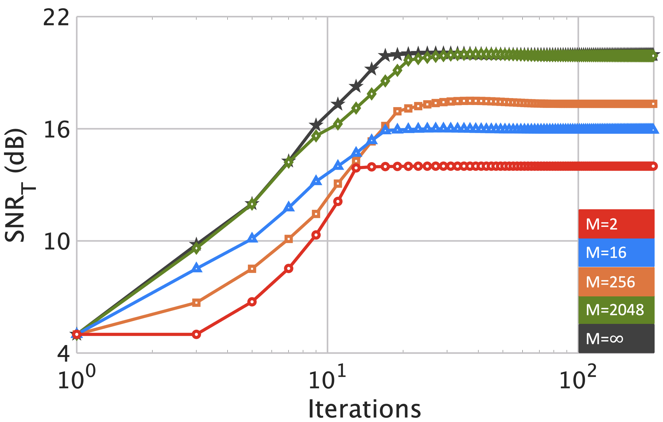
Fig. 2: The optimized SNR${}_{{}_{T}}$(dB) achieved for $\beta=0.5$ , $P_{{}_{T}}=50$ dBm and $P_{{}_{\textrm{IRS}}}=30$ dBm versus $10^{3}$ iterations by jointly designing an active IRS and DFBS precoder matrix.

We validated our model and methods through numerical experiments. Throughout all simulations, we set the number of DFBS antennas to $N=4$. The IRS had $L=16$ reflecting elements and the number of communications users was $K=5$. The radar target was located at DoA $(45^{\degree},45^{\degree})$ and $r_{t}=2500$m with respect to the IRS. The CSI matrices are generated according to the Rician fading channel model [27]. The noise variances at the receivers of all communications users and DFBS were $\sigma_{c}^{2}=0$dBm. Following [30], the MaRLI relaxation parameters were set to $\nu_{1}=1.2$ and $\nu_{2}=10^{-9}$. Fig. 2 shows the achievable $\textrm{SNR}_{{}_{T}}$ with weight factor $\beta=0.5$ through the iterations. At our algorithm, the convergence threshold was set to $\epsilon=10^{-3}$. The proposed algorithm converges to a higher value of SNR${}_{{}_{T}}$ when we increase the number of quantization bits $M$ because the size of the feasible set in $\mathcal{P}_{1}$ grows larger. While MaRLI typically produces high-quality designs over discrete constellations, it is not a monotonic local optimizer [30]. The non-monotonic behavior of the SNR curves is presumably attributed to this characteristic of the MaRLI algorithm.

6 Summary

We considered an IRS-ISAC setup and optimized the performance of both radar and communications receivers through the recently proposed tools in UQP optimization. In particular, our formulation includes the practical setting of quantization in IRS phase-shifts. Numerical experiments with both binarized and densely quantized levels indicate a convergence of our algorithm.

References

• [1] F. Boccardi, R. W. Heath, A. Lozano, T. L. Marzetta, and P. Popovski, “Five disruptive technology directions for 5G,” IEEE Communications Magazine, vol. 52, no. 2, pp. 74–80, 2014.
• [2] K. V. Mishra, M. Shankar, V. Koivunen, B. Ottersten, and S. Vorobyov, “Toward millimeter-wave joint radar communications: A signal processing perspective,” IEEE Signal Processing Magazine, vol. 36, no. 5, pp. 100–114, 2019.
• [3] A. Hassanien, M. G. Amin, E. Aboutanios, and B. Himed, “Dual-function radar communication systems: A solution to the spectrum congestion problem,” IEEE Signal Processing Magazine, vol. 36, no. 5, pp. 115–126, 2019.
• [4] A. M. Elbir, K. V. Mishra, M. B. Shankar, and S. Chatzinotas, “The rise of intelligent reflecting surfaces in integrated sensing and communications paradigms,” IEEE Network, 2022, in press.
• [5] T. Wei, L. Wu, K. V. Mishra, and M. Shankar, “Multi-IRS-aided Doppler-tolerant wideband DFRC system,” arXiv preprint arXiv:2207.02157, 2022.
• [6] T. Wei, L. Wu, K. V. Mishra, and M. B. Shankar, “Multiple IRS-assisted wideband dual-function radar-communication,” in IEEE International Symposium on Joint Communications & Sensing, 2022, pp. 1–5.
• [7] T. Wei, L. Wu, K. V. Mishra, and S. M. Bhavani, “Simultaneous active-passive beamformer design in IRS-enabled multi-carrier DFRC system,” in European Signal Processing Conference, 2022, pp. 1007–1011.
• [8] Z. Wang, X. Mu, and Y. Liu, “STARS enabled integrated sensing and communications,” IEEE Transactions on Wireless Communications, 2023.
• [9] J. A. Hodge, K. V. Mishra, and A. I. Zaghloul, “Intelligent time-varying metasurface transceiver for index modulation in 6G wireless networks,” IEEE Antennas and Wireless Propagation Letters, vol. 19, no. 11, pp. 1891–1895, 2020.
• [10] J. A. Hodge, K. V. Mishra, B. M. Sadler, and A. I. Zaghloul, “Reconfigurable intelligent surfaces for 6G wireless networks using index-modulated metasurface transceivers,” IEEE Journal of Selected Topics in Signal Processing, 2023, in press.
• [11] Z. Esmaeilbeig, K. V. Mishra, A. Eamaz, and M. Soltanalian, “Cramér-Rao lower bound optimization for hidden moving target sensing via multi-IRS-aided radar,” IEEE Signal Processing Letters, vol. 29, pp. 2422–2426, 2022.
• [12] Z. Esmaeilbeig, A. Eamaz, K. V. Mishra, and M. Soltanalian, “Joint waveform and passive beamformer design in multi-IRS aided radar,” in IEEE International Conference on Acoustics, Speech and Signal Processing, 2023, in press.
• [13] Z. Esmaeilbeig, K. V. Mishra, and M. Soltanalian, “IRS-aided radar: Enhanced target parameter estimation via intelligent reflecting surfaces,” in IEEE Sensor Array and Multichannel Signal Processing Workshop, 2022, pp. 286–290.
• [14] B. Zheng, C. You, W. Mei, and R. Zhang, “A survey on channel estimation and practical passive beamforming design for intelligent reflecting surface aided wireless communications,” IEEE Communications Surveys & Tutorials, 2022.
• [15] K. V. Mishra, A. Chattopadhyay, S. S. Acharjee, and A. P. Petropulu, “OptM3Sec: Optimizing multicast IRS-aided multiantenna DFRC secrecy channel with multiple eavesdroppers,” in IEEE International Conference on Acoustics, Speech and Signal Processing, 2022, pp. 9037–9041.
• [16] H. Di, B.and Zhang, L. Song, Y. Li, Z. Han, and H. Poor, “Hybrid beamforming for reconfigurable intelligent surface based multi-user communications: Achievable rates with limited discrete phase shifts,” IEEE Journal on Selected Areas in Communications, vol. 38, no. 8, pp. 1809–1822, 2020.
• [17] C. You, B. Zheng, and R. Zhang, “Intelligent reflecting surface with discrete phase shifts: Channel estimation and passive beamforming,” in IEEE International Conference on Communications, 2020, pp. 1–6.
• [18] H. Gao, K. Cui, C. Huang, and C. Yuen, “Robust beamforming for RIS-assisted wireless communications with discrete phase shifts,” IEEE Wireless Communications Letters, vol. 10, no. 12, pp. 2619–2623, 2021.
• [19] T. Wei, L. Wu, K. V. Mishra, and M. B. Shankar, “IRS-aided wideband dual-function radar-communications with quantized phase-shifts,” in IEEE Sensor Array and Multichannel Signal Processing Workshop, 2022, pp. 465–469.
• [20] X. Wang, Z. Fei, J. Huang, and H. Yu, “Joint waveform and discrete phase shift design for RIS-assisted integrated sensing and communication system under Cramér-Rao bound constraint,” IEEE Transactions on Vehicular Technology, vol. 71, no. 1, pp. 1004–1009, 2021.
• [21] J. A. Hodge, K. V. Mishra, and A. I. Zaghloul, “Deep inverse design of reconfigurable metasurfaces for future communications,” arXiv preprint arXiv:2101.09131, 2021.
• [22] K. V. Mishra, A. M. Elbir, and A. I. Zaghloul, “Machine learning for metasurfaces design and their applications,” in Advances in Electromagnetics Empowered by Machine Learning, ser. Electromagnetic Wave Theory and Applications.   Wiley-IEEE Press, 2023, in press.
• [23] D. Xu, X. Yu, D. W. K. Ng, and R. Schober, “Resource allocation for active irs-assisted multiuser communication systems,” in Asilomar Conference on Signals, Systems, and Computers.   IEEE, 2021, pp. 113–119.
• [24] Y. Zhang, J. Chen, C. Zhong, H. Peng, and W. Lu, “Active IRS-assisted integrated sensing and communication in C-RAN,” IEEE Wireless Communications Letters, vol. 12, no. 3, pp. 411–415, 2023.
• [25] Y. Li and A. Petropulu, “Dual-function radar-communication system aided by intelligent reflecting surfaces,” in IEEE Sensor Array and Multichannel Signal Processing Workshop, 2022, pp. 126–130.
• [26] M. Soltanalian and P. Stoica, “Designing unimodular codes via quadratic optimization,” IEEE Transactions on Signal Processing, vol. 62, no. 5, pp. 1221–1234, 2014.
• [27] Y.-K. Li and A. Petropulu, “Minorization-based low-complexity design for IRS-aided ISAC systems,” arXiv preprint arXiv:2302.11132, 2023.
• [28] A. Eamaz, F. Yeganegi, and M. Soltanalian, “One-bit phase retrieval: More samples means less complexity?” IEEE Transactions on Signal Processing, vol. 70, pp. 4618–4632, 2022.
• [29] A. Eamaz, F. Yeganegi, and M. Soltanalian, “CyPMLI: WISL-minimized unimodular sequence design via power method-like iterations,” in IEEE International Conference on Acoustics, Speech and Signal Processing, 2023, in press.
• [30] A. Eamaz, F. Yeganegi., and M. Soltanalian, “MaRLI: Attack on the discrete-phase WISL minimization problem,” arXiv preprint arXiv, 2023.
• [31] A. Eamaz, F. Yeganegi, K. V. Mishra, and M. Soltanalian, “Near-field low-WISL unimodular waveform design for terahertz automotive radar,” arXiv preprint arXiv:2303.04332, 2023.
• [32] M. Soltanalian and P. Stoica, “Computational design of sequences with good correlation properties,” IEEE Transactions on Signal processing, vol. 60, no. 5, pp. 2180–2193, 2012.
• [33] M. I. Skolnik, Radar handbook, 3rd ed.   McGraw-Hill, 2008.
• [34] Z. Esmaeilbeig, A. Eamaz, K. V. Mishra, and M. Soltanalian, “Moving target detection via multi-IRS-aided OFDM radar,” in IEEE Radar Conference, 2023, in press.
• [35] J. Bezdek and R. Hathaway, “Convergence of alternating optimization,” Neural, Parallel & Scientific Computations, vol. 11, no. 4, pp. 351–368, 2003.
• [36] B. Tang, J. Tuck, and P. Stoica, “Polyphase waveform design for MIMO radar space time adaptive processing,” IEEE Transactions on Signal Processing, vol. 68, pp. 2143–2154, 2020.
• [37] M. Soltanalian, B. Tang, J. Li, and P. Stoica, “Joint design of the receive filter and transmit sequence for active sensing,” IEEE Signal Processing Letters, vol. 20, no. 5, pp. 423–426, 2013.
• [38] C. Van Loan and G. Golub, Matrix computations.   The Johns Hopkins University Press, 1996.
• [39] M. A. Kerahroodi, A. Aubry, A. De Maio, M. Naghsh, and M. Modarres-Hashemi, “A coordinate-descent framework to design low PSL/ISL sequences,” IEEE Transactions on Signal Processing, vol. 65, no. 22, pp. 5942–5956, 2017.