Explainable Semantic Medical Image Segmentation with Style

Abstract

Semantic medical image segmentation using deep learning has recently achieved high accuracy, making it appealing to clinical problems such as radiation therapy. However, the lack of high-quality semantically labelled data remains a challenge leading to model brittleness to small shifts to input data. Most works require extra data for semi-supervised learning and lack the interpretability of the boundaries of the training data distribution during training, which is essential for model deployment in clinical practice. We propose a fully supervised generative framework that can achieve generalisable segmentation with only limited labelled data by simultaneously constructing an explorable manifold during training. The proposed approach creates medical image style paired with a segmentation task driven discriminator incorporating end-to-end adversarial training. The discriminator is generalised to small domain shifts as much as permissible by the training data, and the generator automatically diversifies the training samples using a manifold of input features learnt during segmentation. All the while, the discriminator guides the manifold learning by supervising the semantic content and fine-grained features separately during the image diversification. After training, visualisation of the learnt manifold from the generator is available to interpret the model limits. Experiments on a fully semantic, publicly available pelvis dataset demonstrated that our method is more generalisable to shifts than other state-of-the-art methods while being more explainable using an explorable manifold.

1 Introduction

Convolutional Neural Networks (CNN) Ronneberger et al. (2015); Çiçek et al. (2016); Isensee et al. (2021, 2017); Dai et al. (2022) have been widely used to enhance the segmentation performance for medical images. However, large quantities of training samples are often required by CNN models to avoid over-fitting, which is especially challenging in medical image segmentation, as data scarcity is common due to the extensive time and expertise involved in labelled data acquisition. Semi-supervised and unsupervised generative adversarial methods Li et al. (2017); Xue et al. (2018); Yuan et al. (2019); Rezaei et al. (2019); Gaj et al. (2020); Nie and Shen (2020); Jafari et al. (2019); Dong et al. (2018); Ning et al. (2018); Xing et al. (2020); Decourt and Duong (2020); Lei et al. (2020) have been proposed to address these problems through direct translation between images and masks. While using unlabelled or multi-model data, these methods are still vulnerable to distribution shifts due to the lack of sample diversities. Mixup Zhang et al. (2017) was proposed recently to diversify training samples for deep learning models through linear interpolation of random inputs. However, it still requires human intervention to balance the trade-off between model accuracy and generalizability.

To make segmentation models generalisable to distribution shifts, another group of Generative Adversarial Networks (GAN)-based methods Jin et al. (2018); Chaitanya et al. (2019); Shen et al. (2019); Shin et al. (2018); Huo et al. (2018) have also been proposed to increase the diversity of training samples through augmentation. However, these methods often require a separated segmentation model trained individually with the augmented data and the segmentation training is not directly linked to adversarial learning. While some methods Yuan et al. (2019); Zhao et al. (2018) achieve end-to-end training with both segmentation and augmentation pipelines, they often involve multiple pairs of GANs, which substantially increase the training complexity. Furthermore, none of the mentioned methods are explainable as they lack the style to map the input distribution, hence, it is impossible to build a manifold of the learnt features for model evaluation.

Accurate medical image segmentation is crucial for clinical diagnosis. Hence, it is critical to identify the boundary of valid input distribution for the trained model, as deep learning models tend to be unpredictable when handling inputs outside the training distribution. Confidence learning Decourt and Duong (2020); Nie and Shen (2020), which generates pixel-wise probability maps from discriminator, were proposed to validate the segmentation outputs. However, they cannot identify the learnt distribution due to the lack of style. Style-based methods Abdal et al. (2021); Li et al. (2021); Lee et al. (2022); Chai and Liu (2022); Shi et al. (2020) were proposed to map the input distribution using style by extracting multi-scale features during segmentation. However, they were neither designed to record the learnt distribution nor to visualise them for clinical evaluation. Moreover, none of them explores the possibility of StyleGAN for supervised training with limited medical data only that are semantically labelled.

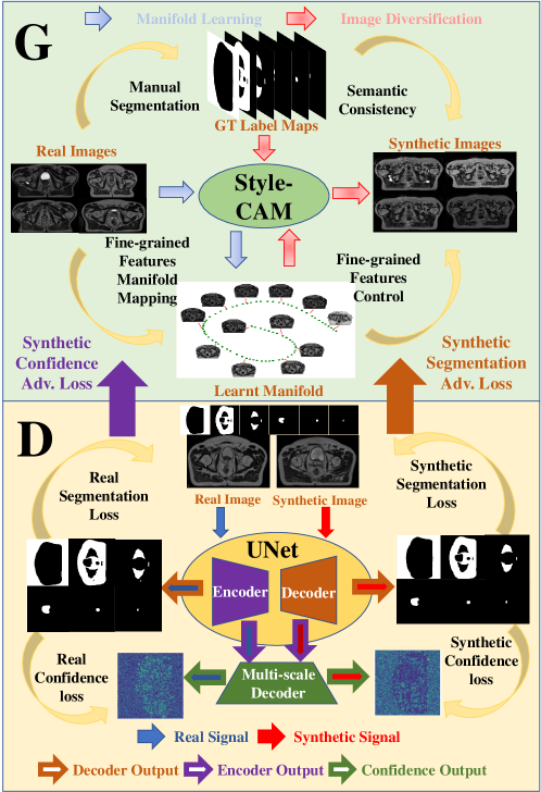
Figure 1: Our GASE framework. Generator G learns an explorable manifold using Style-CAM, which implements style-based modulated convolution with kernel dilation and synthesizes images using the learnt manifold. Discriminator D segments input images semantically while supervising the manifold learning using confidence maps and segmentation outputs.

In this work, we propose Generative Adversarial Segmentation Evolution (GASE), an end-to-end style-based generative model for the semantic segmentation of medical images supervised with limited labelled data. GASE can build a manifold of the learnt input distribution entirely based on the existing labelled data during segmentation training. Instead of augmenting images through the direct translation using training samples, GASE can diversify the samples through the combination of ground truth (GT) masks and extracted features from the learnt manifold. Our aim is to improve the segmentation performance using gradients from both real and diversified samples during segmentation training. To do so, we integrate manifold-based synthesis and semantic segmentation into a generator and a discriminator respectively, while training them in an end-to-end adversarial manner. The generator utilises Modulated Convolution (ModConv) with style Karras et al. (2020a) as a mapping function to build the manifold of the input feature space for synthesis, and the discriminator segments input images with the help of the synthetic samples. Unlike a similar work Shi et al. (2020) which is based on adaptive instance normalization Karras et al. (2019), we introduce Style-CAM, which implements the style-based ModConv with kernel dilation for Context Aggregation Module (CAM) Dai et al. (2022) in our generator, to achieve multi-scale fine-grained features control without any resampling operations. Moreover, the segmentation training process requires no artificial label maps using semantic consistency, thus, preserving the target structural information within the synthetic labelled pairs, which is essential for clinical requirements. The main contributions of this paper are as follows:

1. We propose GASE, a style-based generative model that improves the generalizability of the segmentation model to data shifts by enhancing the diversity of training samples via manifold learning. To the best of our knowledge, GASE is the first method to introduce manifold learning with modulated convolution to supervised semantic medical image segmentation.

2. The proposed model achieves end-to-end training with dual functional networks, a generator that visualises the manifold of learnt distribution for model interpretation, and a discriminator that segments the medical images semantically. We also introduce style-CAM, which implements modulated convolution with kernel dilation for the first time, as far as we know.

3. We demonstrate the effectiveness of GASE with a series of experiments on an open-access labelled pelvis MR dataset with multiple classes. GASE outperforms previous state-of-the-art methods for the chosen dataset, especially for imbalanced classes, and demonstrates better generalisation to input distribution shifts.

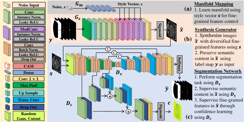
Figure 2: Overall architecture of the proposed GASE. The generator contains two modules, (a) Manifold Mapping $G_{m}$ and (b) Synthesis Generator $G_{s}$. It is used to learn the manifold of input features while diversifying training samples for segmentation based on the learnt manifold. The discriminator consists of two branches, (c) Segmentation branch $D_{s}$ and (d) Confidence Learning branch $D_{c}$. It performs semantic segmentation while guiding manifold learning. $D_{s}$ supervises semantic content in $\hat{x}$ and $D_{c}$ supervises fine features in $\hat{x}$.

2 Related Work

2.1 GAN-based Segmentation Methods

Direct Translation Methods: Since image segmentation can also be considered as image translation between the image domain and the label domain, GAN-based methods, which are noted for high-quality cross-domain image translation, have also been proposed to translate medical images into label maps directly using generator Li et al. (2017); Rezaei et al. (2019); Dong et al. (2018). Segmentation losses for the generator and multi-scale feature losses for the discriminator were added in  Zhao et al. (2018); Xue et al. (2018); Gaj et al. (2020) for extra supervision during training. Multistream translation and segmentation methods Yuan et al. (2019); Xing et al. (2020) based on CycleGANZhu et al. (2017) were also proposed to utilize multi-model data under cycle consistency. Confidence learning Nie and Shen (2020); Decourt and Duong (2020); Jafari et al. (2019), which outputs a pixel-wise probability map from the discriminator, was introduced to supervise the translation on a pixel level. Dual discriminators Lei et al. (2020) were also proposed to supervise the segmentation using both semantic information and contextual environment. However, these methods are vulnerable to model over-fitting due to data scarcity.

Augmentation Methods: To address the problem of data scarcity and make segmentation model generalizable to data shifts, GAN-based methods were also proposed to augment the training samples through image synthesis Jin et al. (2018); Shen et al. (2019). Chaitanya et.al. Chaitanya et al. (2019) used two sub-networks with shared intermediate layers to achieve separate control on the deformation and intensity of augmented images. Artificial label maps were also used to generate synthetic pairs for augmentation by translating them to the target image domain Shin et al. (2018); Shi et al. (2020). CycleGAN-based approach Huo et al. (2018) augments synthetic pairs to train unlabelled data using labelled data from another domain. However, none of the augmentation methods model the input data distribution, hence, lacking generalization capability to distribution shifts.

Style-based Methods: To make segmentation more generalizable to distribution shifts, StyleGANs Karras et al. (2019, 2020a), which learn input distribution by extracting multi-scale features using style, has been recently proposed for segmentation tasks in computer vision  Abdal et al. (2021); Li et al. (2021); Lee et al. (2022). Abdal et.al. Abdal et al. (2021) proposed a style-based unsupervised segmentation network that is trained using synthetic images from two pre-trained generators. Li et.al. Li et al. (2021) tackled semantic segmentation using StyleGAN by modelling the joint image-label distribution for unlabeled images using limited labelled ones in a semi-supervised manner. Chai et.al. Chai and Liu (2022) also proposed a semi-supervised method to segment medical images by generating attention-based label maps during a two-stage hierarchical synthesis using style-based generators.

3 Methodology

3.1 Definition and Overview

We denote the limited labelled dataset as $S=\{x,y\}$, where $x\in\mathbb{R}^{B\times H\times W\times 1}$ represents a batch of images under real image distribution $P_{data}(x)$ with batch size $B$, $y\in\mathbb{R}^{B\times H\times W\times C}$ is the corresponding one-hot encoded GT label batch with $C$ classes. The overall architecture of GASE is shown in Fig. 2. The generator $G$ contains two sub-models: manifold mapping $G_{m}:z\rightarrow s$, which generates style vectors $s\in\mathbb{R}^{1\times P}$ given noise vectors $z\in\mathbb{R}^{1\times L}$, and the synthesis generator $G_{s}:(y,s)\rightarrow\hat{x}$, where $\hat{x}$ represents synthesized images from a recovered fake distribution $P_{fake}(x)$ after manifold learning. The discriminator $D:(x,\hat{x})\rightarrow(\hat{y}_{x},\hat{y}_{\hat{x}},c_{x},c_{\hat{x}})$ is a segmentation network which takes both $x$ and $\hat{x}$ as input and outputs predicted label map $\hat{y}\in\mathbb{R}^{B\times H\times W\times C}$ and confidence map $c\in\mathbb{R}^{B\times H\times W\times 1}$ for both inputs simultaneously.

Overall, we propose a style-based $G$ that controls the features within $\hat{x}$ by injecting learnable $s$ into the intermediate layers of $G_{s}$ using ModConv. As $G$ gets better at synthesizing $\hat{x}$, different $s$ will be mapped to a manifold that recovers the distribution of input features. By using $y$ as input for $G$ and outputting $\hat{y}$ from $D$, semantic consistency can be achieved during adversarial training so the semantic content from input $y$ will be preserved in the corresponding $\hat{x}$. Such consistency will make manifold mapping focus more on fine-grained features, such as pixel density and contrast, and preserve global features, such as real semantic information from $y$. The whole manifold mapping process is supervised by the pixel-wise probability map $c$ from $D$ through adversarial training. By feeding different $s$, extracted from the learnt manifold, with the same $y$ into $G$, images with the same semantic content as $y$ but diversified fine-grained features could be synthesized, thus, forming a new synthetic pair $(\hat{x},y)$ that shares the same label map with the corresponding real pair $(x,y)$. During segmentation training, gradient information from the $(\hat{x},y)$ is progressively propagated along with the $(x,y)$ as the $P_{fake}(x)$ better resembles the $P_{data}(x)$. Once the training is done, $G$ can be used to visualize the learnt manifold by projecting $s$ into the lower dimension with the corresponding $\hat{x}$. We now discuss the technical details for each part of the proposed architecture.

3.2 Analyszing Role of Style-based Generator

Two strategies are taken to make the segmentation task more generalizable to distribution shifts under limited training samples. First, we want to diversify the training samples while preserving the semantic content from GT label maps. Doing so will avoid using artificial label maps when generating synthetic labelled pairs, preventing augmentation leakage Karras et al. (2020b). Second, we want to make the model interpretable so the training data distribution can be mapped into a manifold for visualization. Based on these ideas, we proposed a style-based generator with two sub-models, manifold mapping $G_{m}$ and synthesis generator $G_{s}$

Manifold Mapping, $G_{m}$: As shown in Fig. 2a, $G_{m}$ is designed to generate style vectors $s$ that control the fine-grained features within the $\hat{x}$. Given a Gaussian noise vector $z$, $G_{m}$ will transform $z$ into style vector $s$ using consecutive dense layers. Each $s$ is learned during training to match a specific fine-grained feature from the input distribution. However, due to the limited training samples, over-fitting could easily occur when all $z$ are transformed into the same $s$. To address this, we propose a penalizing term when training $G$ by regularizing the transformation as follows:

$$\mathcal{L}_{Gp}(y,z_{1},z_{2};\theta_{G_{m},G_{s}})=\frac{\lambda_{1}}{\mathcal{L}_{mse}(\hat{x}_{1},\hat{x}_{2})+\lambda_{2}},$$ (1)

where $\hat{x}_{1}$ and $\hat{x}_{2}$ are two synthetic images generated using different noise input $z_{1}$ and $z_{2}$. Taking the reciprocal of Mean Squared Error (MSE) between two synthetic images, a large loss will be applied when similar images are generated with different $z$. By doing so, $s$ will be forced to learn the correlation among different input features, building a manifold with diversified features that ensemble $P_{data}(x)$ as well as possible. Values of 0.01 and 0.001 are chosen for $\lambda_{1}$ and $\lambda_{2}$, to limit the maximum penalty with a sharp gradient. Moreover, to avoid sparse distribution of $s$ and distribute them evenly across the manifold, spectral normalization Miyato et al. (2018) is applied to each dense layer in $G_{m}$ to mitigate large gradient of $\theta_{G_{m}}$ during training.

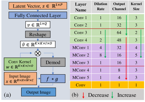
Figure 3: a) Structure of the modified modulated convolution layer. b) Details for convolution layers within synthesis generator $G_{m}$. Layers between two red lines represent the layers within the context aggregation module (CAM).

Modulated Convolution Layer: To map $s$ from $G_{m}$ to various fine-grained features within input images through manifold learning, a modified ModConv layer shown in Fig. 3a is designed to modulate convolution kernel using $s$. Unlike the original ModConv layer Karras et al. (2020a), which uses different $s$ for different layers during multi-scale features extraction, the same $s$ is used instead to match a unique feature during manifold learning. To achieve this, a dense operation is firstly applied to transform $s\in\mathbb{R}^{1\times P}$ to $v\in\mathbb{R}^{1\times Q}$, so the vector size $Q$ matches the number of trainable weights within convolution kernel $w\in\mathbb{R}^{K\times K\times I\times O}$, where K is the kernel size, I and O represent layer input and output channel numbers respectively. After reshaping $v$, $\hat{v}\in\mathbb{R}^{K\times K\times I\times O}$ is used to modulate convolution kernel through simple multiplication: $\hat{w}=w\cdot\hat{v}$. Finally, the same demodulation procedure in Karras et al. (2020a) is implemented to normalize the scaled kernel weights, and the resulting kernel is used to conduct convolution operation with layer input.

Synthesis Generator, $G_{s}$: As illustrated in Fig. 2b, multiple standard convolution blocks are first applied to learn the general shape information of the input masks. Then a modified version of CAM Dai et al. (2022) is implemented with ModConv layers to modify the fine-grained features on multiple scales under a larger receptive field without any re-sampling operations. As shown in Fig. 3b, different to the original CAM, the kernel sizes of the convolution layers are increased gradually to expand the regions that could be modulated by $s$. Concurrently, the number of output channels for each layer is progressively decreased to avoid model over-parameterization. In this supervised learning, other than the penalty term introduced in Eq. 1, all other training signals for $G_{s}$ only come from the $D$. By taking the same $y$ and different $s$, $G_{s}$ can diversify the training samples with various fine-grained features while preserving the semantic content from $y$.

3.3 Segmentation Discriminator with Supervision

As illustrated in Fig. 2c, the proposed $D$ consists of two branches, a segmentation branch $D_{s}$ and a confidence learning branch $D_{c}$. $D_{s}$ is the backbone of GASE that performs image segmentation tasks. At the same time, it also supervises semantic content of $\hat{x}$ during $G$ training. $D_{c}$ is designed to supervise the fine-grained features within the $\hat{x}$ through confidence learning.

Discriminator for Segmentation: The $D_{s}$ is designed based on the 2D-UNet Ronneberger et al. (2015) with additional dropout for image segmentation. By training $D_{s}$ with the synthetic pair $(\hat{x},y)$ and the real pair $(x,y)$ simultaneously, the different fine-grained features with the same label map between $x$ and $\hat{x}$ will force $D_{s}$ to handle more diversified features during segmentation, hence, becoming more robust to distribution shifts. The loss for such counter pairs is defined as:

$$\mathcal{L}_{Ds}(x,\hat{x}:\theta_{D_{s}})=\\ \mathcal{L}_{dsl}(D_{s}(x),y)+\lambda_{3}\cdot\gamma\cdot\mathcal{L}_{dsl}(D_{s}(\hat{x}),y),$$ (2)

where $\mathcal{L}_{dsl}$ is the weighted Dice Squared Loss (DSL) proposed in Dai et al. (2022) and $\lambda_{3}$ is a weighting factor which limits the maximum signal provided by the $\hat{x}$. To limit the second loss term when the quality of $\hat{x}$ is low at the initial training stage, a scheduled weighting factor $\gamma$, which starts from zero, is increased progressively based on the inverse of polynomial decay until reaching one when $G$ is capable of synthesizing realistic $\hat{x}$. Moreover, to give $G$ more freedom during synthesis and balance the training between $G$ and $D$, we designed a random cutout layer with Gaussian noise to inject local randomness into the input of $D$ ( Fig. 2c). Compared to the original random cutout DeVries and Taylor (2017), which uses the constant value in the cutout region, Gaussian noise is used instead for better gradient propagation.

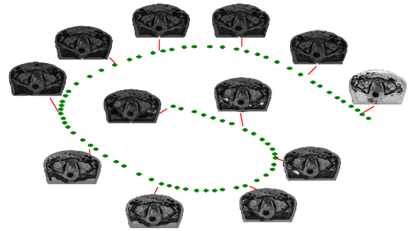
Figure 4: Visualization of the manifold learnt by GASE during segmentation training. Green dots represent the sampled style vectors projected onto a 2D plane. Each style vector represents a specific fine-grained feature shown in the provided images. Such a manifold can be used to explain the segmentation training.

Discriminator for Supervision: While getting better at the segmentation task, $D_{s}$ also supervises the semantic content within $\hat{x}$ by propagating segmentation loss between $y$ and $\hat{y}$ to $G$ during adversarial training, which is defined as:

$$\mathcal{L}_{Gs}(y,z;\theta_{G_{m},G_{s}})=\mathcal{L}_{dsl}(D_{s}(\hat{x}),y).$$ (3)

By minimizing $\mathcal{L}_{Gs}$, $G$ is forced to synthesize images with the same semantic content as $y$, therefore, achieving semantic consistency between $\hat{x}$ and $y$. To supervise fine-grained features within $\hat{x}$, the encoder of $D_{s}$ also extracts features from the input images for confidence branch $D_{c}$. Compared to the standalone encoder proposed in Xue et al. (2018), the features extracted in our approach are constrained by the multi-class shape information from $y$ as the encoder is trained under the guidance of the decoder, which performs shape reconstruction. Such shape-constrained features will provide class information to $D_{c}$ when generating confidence map $c$.

As illustrated in Fig. 2c, $D_{c}$ uses multi-scale features extracted by the encoder of $D_{s}$ as input. It supervises $G$ by providing an adversarial loss based on the generated probability map $c\in\mathbb{R}^{B\times H\times W\times 1}$ that indicates the pixel-wise realness of fine-grained features within $\hat{x}$. Due to the down-sampling operations within the encoder of $D_{s}$, large-scaled features will cover more local information, whereas lower-scaled features will contain more global information. By aggregating the multi-scale features, the generated confidence map will better distinguish the ’real’ or ’fake’ features based on local and global information. The confidence loss when training $D_{c}$ is defined as:

$$\mathcal{L}_{Dc}(x,\hat{x};\theta_{Dc})=\mathcal{L}_{bce}(c_{x},(1-\zeta))+\mathcal{L}_{bce}(c_{\hat{x}},\zeta),$$ (4)

where $\mathcal{L}_{bce}$ is the binary cross-entropy loss, $c_{x}$ and $c_{\hat{x}}$ are the confidence maps generated with $x$ and $\hat{x}$ respectively, $\zeta$ is a small Gaussian noise used to provide better gradient. The adversarial confidence loss for $G$ is defined as:

$$\mathcal{L}_{Gc}(y,z;\theta_{G_{m},G_{s}})=\mathcal{L}_{bce}(c_{\hat{x}},(1-\zeta)).$$ (5)

3.4 Training Losses Details

During the training, $G$ and $D$ will be trained iteratively for specified epochs. We define the hybrid adversarial loss function for $G$ as:

$$\mathcal{L}_{G}\left(\theta_{G_{m}},\theta_{G_{s}}\right)=\beta\mathcal{L}_{Gs}+\mathcal{L}_{Gc}+\mathcal{L}_{Gp},$$ (6)

where $\beta$ is set to 2 to enforce the semantic consistency. The hybrid loss function defined for $D$ is:

$$\mathcal{L}_{D}\left(\theta_{D_{s}},\theta_{D_{c}}\right)=\mathcal{L}_{Ds}+\mathcal{L}_{Dc}.$$ (7)

4 Experiments

Table 1: The ablation study for each module of the proposed GASE. The modules are $G_{s}$: synthesis generator, $G_{m}$: manifold mapping, $D$: segmentation discriminator and Mixup: mixup augmentation technique.

$G_{s}$

$G_{m}$

D

Mixup

DSC

HD

MSD

Bladder

Rectum

Prostate

Bladder

Rectum

Prostate

Bladder

Rectum

Prostate

✓

0.91 ± 0.07

0.93 ± 0.05

0.72 ± 0.16

10.2 ± 13.9

4.70 ± 11.4

8.08 ± 5.22

1.76 ± 1.36

1.13 ± 1.67

3.61 ± 1.83

✓

✓

0.91 ± 0.07

0.93 ± 0.05

0.73 ± 0.19

12.0 ± 22.1

4.64 ± 9.20

9.89 ± 19.1

1.75 ± 2.14

1.16 ± 1.69

4.28 ± 14.9

✓

✓

0.92 ± 0.07

0.92 ± 0.07

0.74 ± 0.16

7.78 ± 15.2

4.73 ± 5.19

8.19 ± 4.22

1.44 ± 0.93

1.25 ± 1.17

3.46 ± 1.66

✓

✓

✓

0.92 ± 0.06

0.93 ± 0.02

0.75 ± 0.17

6.67 ± 7.79

5.14 ± 8.75

8.52 ± 6.09

1.37 ± 0.83

1.21 ± 1.23

3.31 ± 1.91

Datasets: Due to the lack of public medical datasets that are fully segmented semantically with multiple classes (including body and bone), an open-access magnetic resonance (MR) dataset of the pelvis Dowling et al. (2015) was used for our experiment. The 3D pelvis dataset consists of 211 MR examinations acquired each week longitudinally for up to 8 weeks for a cohort of 38 patients diagnosed with prostate cancer. Single 3D CT image was also acquired at baseline for each patient and used for cross-modality evaluation. All images are manually segmented into six classes: background, pelvic cavity, bone, bladder, prostate and rectum. Each examination has an image size of $256\times 256\times 256$ voxels with a resolution of $1.68\times 1.68\times 1.56$ mm.

Preprocessing: To make the 3D images suitable for our 2D models, 2D slices containing all classes were extracted from each volume along the axial axis after bias-field correction Tustison et al. (2010). The resulting 1775 slices were then used as our training set after being normalised to $[0,1]$ in intensity values with zero mean and standard deviation. Finally, three-fold cross-validation studies were conducted by randomly splitting the extracted slices into three subsets (751/656/368) on a patient basis. The testing set from each fold was also used as the validation set during training. All results reported in this paper are the averaged 3-fold cross-validation results using the testing set only.

Implementation: We employed the proposed model with the Tensorflow v2.9.0 framework on NVIDIA Volta V100 GPU with 32GB of memory. All models were trained for 2000 epochs with a batch size of 15. The model with the best validation performance during training was saved for evaluation. Adam optimizers with initial learning rates of $5\times 10^{-3}$ and $1\times 10^{-3}$ were chosen for the training of $G$ and $D$ respectively. Furthermore, the polynomial decay was used to decrease both learning rates with a power of two after each epoch until reaching zero at the end of training.

Evaluation Metrics: Three evaluation metrics were adopted in this experiment. The Dice Similarity Coefficient (DSC) was used to access the overlapping ratios between the $\hat{y}$ and $y$. Hausdorff Distance (HD) and Mean Surface Distance (MSD) values were used to calculate the maximum and averaged surface distance error between the anatomical boundaries of the $\hat{y}$ and $y$.

4.1 Ablation Studies

Fig. 4 visualises the manifold of fine-grained features of the inputs learnt by $G$ during adversarial training. To visualise such a manifold, noise vectors, $z$, were randomly chosen to generate different style vectors $s$ using $G_{m}$. The manifold was then obtained by projecting the generated $s$ onto a 2D plane using T-SNE Van der Maaten and Hinton (2008). The corresponding synthetic images $\hat{x}$ used for manifold visualisation were then generated by combining different $s$ with the same label input $y$ using $G_{s}$ and were placed in the 2D plane based on the location of their corresponding $s$. As demonstrated in Fig. 4, all synthetic images have the same semantic content with fine-grained features, such as pixel density and contrast, gradually changing along the learnt manifold. This indicates that the proposed model successfully explores the possible combinations of fine-grained features extracted from the limited dataset, which are then used to improve the segmentation performance by diversifying the training samples based on the learnt manifold. Such visualisation could also be used to explain the trained model by displaying all valid inputs that $D$ has seen during segmentation training.

Tab. 1 gives the ablation study of each module in our approach. To evaluate the baseline performance of the segmentation model $D_{s}$, we trained it using the limited labelled data both with and without mixup Zhang et al. (2017) augmentation. As shown in Tab. 1, the diversified training samples after mixup improve the performance of the $D_{s}$ as expected. To evaluate the performance of our model with and without the ModConv layer using $s$ from $G_{m}$, we separated $G_{m}$ from $G_{s}$ by replacing the ModConv layer with the standard convolution. As shown in the table, training $D$ with $G_{s}$ makes the segmentation performance worse than the $D$ without it. Such results are expected as the synthesized images lose the fine-grained feature control due to the missing manifold learnt by $G_{m}$. However, when we combined $G_{s}$ with $G_{m}$ using ModConv during $D$ training, the segmentation performance increases substantially and even surpasses $D$ with mixup for both DSC and MSD. Such results indicate that our method successfully improves the segmentation performance by diversifying the training samples based on the learnt manifold.

Table 2: Comparison of quantitative results for GASE in semantic segmentation averaged cross-validation testing results.

Region	Mean Metric	GASE	nnUnet Isensee et al. (2021)	ConfiGAN Nie and Shen (2020)	IUNET Isensee et al. (2017)	UNET Ronneberger et al. (2015)
Rectum	DSC	0.94 ± 0.04	0.92 ± 0.06	0.88 ± 0.09	0.87 ± 0.10	0.91 ± 0.07
	HD(mm)	4.29 ± 6.87	5.23 ± 11.9	7.41 ± 7.09	13.8 ± 25.0	9.17 ± 19.3
	MSD(mm)	1.11 ± 0.98	1.63 ± 4.75	1.93 ± 1.78	2.68 ± 3.48	1.96 ± 3.00
Prostate	DSC	0.78 ± 0.16	0.76 ± 0.16	0.74 ± 0.18	0.71 ± 0.17	0.71 ± 0.23
	HD(mm)	8.21 ± 9.33	7.37 ± 7.08	10.5 ± 17.4	16.1 ± 32.0	23.7 ± 62.5
	MSD(mm)	3.30 ± 6.01	3.39 ± 5.20	4.78 ± 15.3	5.64 ± 16.5	18.2 ± 60.6
Bladder	DSC	0.90 ± 0.10	0.90 ± 0.11	0.82 ± 0.17	0.85 ± 0.17	0.85 ± 0.17
	HD(mm)	8.43 ± 9.95	8.34 ± 14.9	55.7 ± 28.5	20.5 ± 32.6	15.7 ± 27.5
	MSD(mm)	1.71 ± 1.66	2.16 ± 6.36	9.26 ± 16.6	4.57 ± 13.0	4.47 ± 19.9
Bone	DSC	0.93 ± 0.02	0.93 ± 0.02	0.90 ± 0.03	0.90 ± 0.04	0.91 ± 0.03
	HD(mm)	21.1 ± 14.8	15.9 ± 12.7	41.8 ± 17.7	28.7 ± 17.8	25.9 ± 17.6
	MSD(mm)	2.08 ± 0.80	1.84 ± 0.56	3.95 ± 1.86	3.02 ± 1.41	2.51 ± 1.33

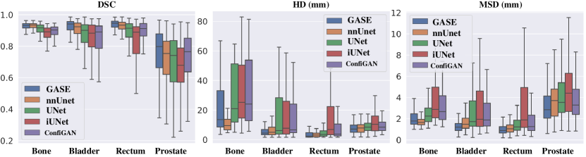
Figure 5: Testing results of GASE and the chosen models for the validation fold containing extreme data shifts within its testing set due to extreme abdominal body fat and non-normal bladder contrast. The outliers are removed from the plot.

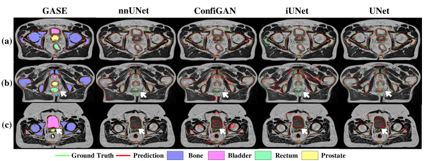
Figure 6: Illustration of segmentation results for three cases. a) Easy case when all classes have distinct features. b) Difficult case when all classes have intricate features, especially for the imbalanced classes like the rectum and prostate. c) Data shifting case when the patient has a large amount of abdominal fat and abnormal bladder contrast. Segmentation outlines are drawn in red (Prediction) and green (GT).

4.2 Comparison with State-of-the-Art Methods

State-of-the-art supervised methods were chosen to evaluate the performance of our GASE with limited labelled data only. Popular UNet Ronneberger et al. (2015) and improved UNet Isensee et al. (2017) were chosen as the baseline models for comparison. GASE was also compared with nnUNet Isensee et al. (2021) directly, which is an automatic configuration pipeline based on UNet. GAN-based model with confidence learning Nie and Shen (2020) was chosen as the related generative model for comparison.

Tab. 2 shows the quantitative results for the chosen models. GASE performs the best in terms of DSC and HD for non-rigid components such as the bladder, prostate and rectum segmentation. It performs slightly worse than nnUnet on HD and does not perform as well as nnUnet for the rigid component such as bone. The reason is that fine-grained features of the bone are relatively consistent across all training samples, which limits the features that could be diversified during image synthesis, hence, the segmentation accuracy of the bone. The visualisation of segmentation results is also demonstrated in Fig. 6. As shown in Fig. 6a, all models achieve accurate segmentation results when all classes have distinct features such as density, contrast and shape from each other. However, as the features among classes become more intricate, for example, the smaller bladder, multiple sections of bone, and similar features between rectum and prostate, shown in Fig. 6b. GASE is the only model that can consistently produce accurate label maps for all classes, especially the rectum, which is missing in all other models’ results. Moreover, it is found that GASE performs substantially better than other models for one validation fold whose testing set contains one case with extreme data shifts compared to the corresponding training set. The results are displayed in Fig. 5. As demonstrated in Fig. 6c, the extreme case has an abnormal bladder contrast with substantially more body fat compared to images in a) and b), and only GASE and nnUnet could segment all classes properly. However, by comparing the segmented prostate from both models, GASE successfully mitigates the misclassified prostate within the bladder. The nnUnet, on the other hand, falsely segments a large portion of the bladder as the prostate due to the unseen bladder contrast. Both quantitative and qualitative results indicate that our GASE is more generalisable to distribution shifts than other models.

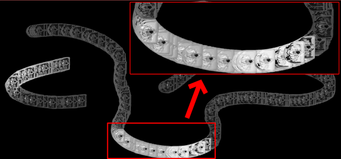
Figure 7: The visualisation of manifold learnt by GASE when mixing both MRI and CT images as training samples. The red section shows the location of CT images within the manifold. This figure is similar to Fig. 4 but with all images plotted.

4.3 Generalisation to Input Diversity

To test how generalisable the GASE is when training with a more complex dataset, we trained GASE and nnUnet with both MRI and CT images provided and tested them with the original MR testing set. As shown in Fig. 7, GASE successfully distinguishes the CT from MR images by grouping images with CT features together within the learnt manifold. Fig. 8 illustrates that while the extra CT data decreases the performance of nnUnet, the accuracy of GASE increases slightly for DSC and HD. Therefore, unlike the nnUnet, whose performance is easily influenced by the quality of the inputs, GASE is more generalisable to a diversified training set due to the learnt manifold, providing consistent accuracy even if the complexity of the training set is increased.

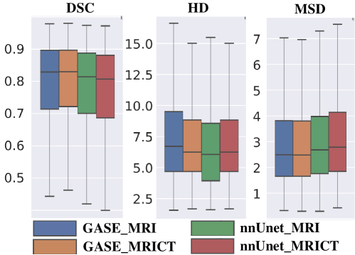
Figure 8: Box-plot results for GASE and nnUnet when both models are trained with a mixture of MRI and CT images. With the extra CT images as input, GASE’s performance increases slightly while nnUnet’s performance decreases.

5 Conclusion

In this paper, we propose GASE, a style-based generative framework that achieves supervised segmentation that generalises to distribution shifts with limited labelled data. We proposed a synthesis generator and a segmentation discriminator trained in a novel way using adversarial losses incorporating confidence. Our GASE learns the manifold for segmentation with the discriminator guiding the manifold learning by supervising semantic content and fine-grained features within the synthetic samples. This manifold can be visualised to explain the trained model by demonstrating the features that the discriminator sees during segmentation training. Our GASE outperforms four state-of-the-art methods on an open-access semantic pelvis MR data set with substantially higher accuracy when handling images with extreme distribution shifts. GASE also shows consistent performance regardless of the increased complexity of the training set, but requires fully semantically labelled datasets for optimal performance.

References

- Ronneberger et al. [2015] Olaf Ronneberger, Philipp Fischer, and Thomas Brox. U-net: Convolutional networks for biomedical image segmentation. In International Conference on Medical image computing and computer-assisted intervention, pages 234–241. Springer, 2015.
- Çiçek et al. [2016] Özgün Çiçek, Ahmed Abdulkadir, Soeren S Lienkamp, Thomas Brox, and Olaf Ronneberger. 3d u-net: learning dense volumetric segmentation from sparse annotation. In International conference on medical image computing and computer-assisted intervention, pages 424–432. Springer, 2016.
- Isensee et al. [2021] Fabian Isensee, Paul F Jaeger, Simon AA Kohl, Jens Petersen, and Klaus H Maier-Hein. nnu-net: a self-configuring method for deep learning-based biomedical image segmentation. Nature methods, 18(2):203–211, 2021.
- Isensee et al. [2017] Fabian Isensee, Philipp Kickingereder, Wolfgang Wick, Martin Bendszus, and Klaus H Maier-Hein. Brain tumor segmentation and radiomics survival prediction: Contribution to the brats 2017 challenge. In International MICCAI Brainlesion Workshop, pages 287–297. Springer, 2017.
- Dai et al. [2022] Wei Dai, Boyeong Woo, Siyu Liu, Matthew Marques, Craig Engstrom, Peter B Greer, Stuart Crozier, Jason A Dowling, and Shekhar S Chandra. Can3d: Fast 3d medical image segmentation via compact context aggregation. Medical Image Analysis, 82:102562, 2022.
- Li et al. [2017] Zeju Li, Yuanyuan Wang, and Jinhua Yu. Brain tumor segmentation using an adversarial network. In International MICCAI brainlesion workshop, pages 123–132. Springer, 2017.
- Xue et al. [2018] Yuan Xue, Tao Xu, Han Zhang, L Rodney Long, and Xiaolei Huang. Segan: adversarial network with multi-scale l1 loss for medical image segmentation. Neuroinformatics, 16(3):383–392, 2018.
- Yuan et al. [2019] Wenguang Yuan, Jia Wei, Jiabing Wang, Qianli Ma, and Tolga Tasdizen. Unified attentional generative adversarial network for brain tumor segmentation from multimodal unpaired images. In International Conference on Medical Image Computing and Computer-Assisted Intervention, pages 229–237. Springer, 2019.
- Rezaei et al. [2019] Mina Rezaei, Haojin Yang, Konstantin Harmuth, and Christoph Meinel. Conditional generative adversarial refinement networks for unbalanced medical image semantic segmentation. In 2019 IEEE winter conference on applications of computer vision (WACV), pages 1836–1845. IEEE, 2019.
- Gaj et al. [2020] Sibaji Gaj, Mingrui Yang, Kunio Nakamura, and Xiaojuan Li. Automated cartilage and meniscus segmentation of knee mri with conditional generative adversarial networks. Magnetic resonance in medicine, 84(1):437–449, 2020.
- Nie and Shen [2020] Dong Nie and Dinggang Shen. Adversarial confidence learning for medical image segmentation and synthesis. International journal of computer vision, 128(10):2494–2513, 2020.
- Jafari et al. [2019] Mohammad H Jafari, Hany Girgis, Amir H Abdi, Zhibin Liao, Mehran Pesteie, Robert Rohling, Ken Gin, Terasa Tsang, and Purang Abolmaesumi. Semi-supervised learning for cardiac left ventricle segmentation using conditional deep generative models as prior. In 2019 IEEE 16th International Symposium on Biomedical Imaging (ISBI 2019), pages 649–652. IEEE, 2019.
- Dong et al. [2018] Nanqing Dong, Michael Kampffmeyer, Xiaodan Liang, Zeya Wang, Wei Dai, and Eric Xing. Unsupervised domain adaptation for automatic estimation of cardiothoracic ratio. In International conference on medical image computing and computer-assisted intervention, pages 544–552. Springer, 2018.
- Ning et al. [2018] Yang Ning, Zhongyi Han, Li Zhong, and Caiming Zhang. Automated pancreas segmentation using recurrent adversarial learning. In 2018 IEEE International Conference on Bioinformatics and Biomedicine (BIBM), pages 927–934. IEEE, 2018.
- Xing et al. [2020] Jie Xing, Zheren Li, Biyuan Wang, Yuji Qi, Bingbin Yu, Farhad G Zanjani, Aiwen Zheng, Remco Duits, and Tao Tan. Lesion segmentation in ultrasound using semi-pixel-wise cycle generative adversarial nets. IEEE/ACM transactions on computational biology and bioinformatics, 2020.
- Decourt and Duong [2020] Colin Decourt and Luc Duong. Semi-supervised generative adversarial networks for the segmentation of the left ventricle in pediatric mri. Computers in Biology and Medicine, 123:103884, 2020.
- Lei et al. [2020] Baiying Lei, Zaimin Xia, Feng Jiang, Xudong Jiang, Zongyuan Ge, Yanwu Xu, Jing Qin, Siping Chen, Tianfu Wang, and Shuqiang Wang. Skin lesion segmentation via generative adversarial networks with dual discriminators. Medical Image Analysis, 64:101716, 2020.
- Zhang et al. [2017] Hongyi Zhang, Moustapha Cisse, Yann N Dauphin, and David Lopez-Paz. mixup: Beyond empirical risk minimization. arXiv preprint arXiv:1710.09412, 2017.
- Jin et al. [2018] Dakai Jin, Ziyue Xu, Youbao Tang, Adam P Harrison, and Daniel J Mollura. Ct-realistic lung nodule simulation from 3d conditional generative adversarial networks for robust lung segmentation. In International Conference on Medical Image Computing and Computer-Assisted Intervention, pages 732–740. Springer, 2018.
- Chaitanya et al. [2019] Krishna Chaitanya, Neerav Karani, Christian F Baumgartner, Anton Becker, Olivio Donati, and Ender Konukoglu. Semi-supervised and task-driven data augmentation. In International conference on information processing in medical imaging, pages 29–41. Springer, 2019.
- Shen et al. [2019] Tianyu Shen, Chao Gou, Fei-Yue Wang, Zilong He, and Weiguo Chen. Learning from adversarial medical images for x-ray breast mass segmentation. Computer methods and programs in biomedicine, 180:105012, 2019.
- Shin et al. [2018] Hoo-Chang Shin, Neil A Tenenholtz, Jameson K Rogers, Christopher G Schwarz, Matthew L Senjem, Jeffrey L Gunter, Katherine P Andriole, and Mark Michalski. Medical image synthesis for data augmentation and anonymization using generative adversarial networks. In International workshop on simulation and synthesis in medical imaging, pages 1–11. Springer, 2018.
- Huo et al. [2018] Yuankai Huo, Zhoubing Xu, Hyeonsoo Moon, Shunxing Bao, Albert Assad, Tamara K Moyo, Michael R Savona, Richard G Abramson, and Bennett A Landman. Synseg-net: Synthetic segmentation without target modality ground truth. IEEE transactions on medical imaging, 38(4):1016–1025, 2018.
- Zhao et al. [2018] Miaoyun Zhao, Li Wang, Jiawei Chen, Dong Nie, Yulai Cong, Sahar Ahmad, Angela Ho, Peng Yuan, Steve H Fung, Hannah H Deng, et al. Craniomaxillofacial bony structures segmentation from mri with deep-supervision adversarial learning. In International conference on medical image computing and computer-assisted intervention, pages 720–727. Springer, 2018.
- Abdal et al. [2021] Rameen Abdal, Peihao Zhu, Niloy J Mitra, and Peter Wonka. Labels4free: Unsupervised segmentation using stylegan. In Proceedings of the IEEE/CVF International Conference on Computer Vision, pages 13970–13979, 2021.
- Li et al. [2021] Daiqing Li, Junlin Yang, Karsten Kreis, Antonio Torralba, and Sanja Fidler. Semantic segmentation with generative models: Semi-supervised learning and strong out-of-domain generalization. In Proceedings of the IEEE/CVF Conference on Computer Vision and Pattern Recognition, pages 8300–8311, 2021.
- Lee et al. [2022] Seunghun Lee, Wonhyeok Choi, Changjae Kim, Minwoo Choi, and Sunghoon Im. Adas: A direct adaptation strategy for multi-target domain adaptive semantic segmentation. In Proceedings of the IEEE/CVF Conference on Computer Vision and Pattern Recognition, pages 19196–19206, 2022.
- Chai and Liu [2022] Lu Chai and Qinyuan Liu. Semi-supervised semantic segmentation of class-imbalanced images: A hierarchical self-attention generative adversarial network. In 2022 7th International Conference on Image, Vision and Computing (ICIVC), pages 398–404. IEEE, 2022.
- Shi et al. [2020] Haoqi Shi, Junguo Lu, and Qianjun Zhou. A novel data augmentation method using style-based gan for robust pulmonary nodule segmentation. In 2020 Chinese Control and Decision Conference (CCDC), pages 2486–2491. IEEE, 2020.
- Karras et al. [2020a] Tero Karras, Samuli Laine, Miika Aittala, Janne Hellsten, Jaakko Lehtinen, and Timo Aila. Analyzing and improving the image quality of stylegan. In Proceedings of the IEEE/CVF conference on computer vision and pattern recognition, pages 8110–8119, 2020a.
- Karras et al. [2019] Tero Karras, Samuli Laine, and Timo Aila. A style-based generator architecture for generative adversarial networks. In Proceedings of the IEEE/CVF conference on computer vision and pattern recognition, pages 4401–4410, 2019.
- Zhu et al. [2017] Jun-Yan Zhu, Taesung Park, Phillip Isola, and Alexei A Efros. Unpaired image-to-image translation using cycle-consistent adversarial networks. In Proceedings of the IEEE international conference on computer vision, pages 2223–2232, 2017.
- Karras et al. [2020b] Tero Karras, Miika Aittala, Janne Hellsten, Samuli Laine, Jaakko Lehtinen, and Timo Aila. Training generative adversarial networks with limited data. Advances in Neural Information Processing Systems, 33:12104–12114, 2020b.
- Miyato et al. [2018] Takeru Miyato, Toshiki Kataoka, Masanori Koyama, and Yuichi Yoshida. Spectral normalization for generative adversarial networks. arXiv preprint arXiv:1802.05957, 2018.
- DeVries and Taylor [2017] Terrance DeVries and Graham W Taylor. Improved regularization of convolutional neural networks with cutout. arXiv preprint arXiv:1708.04552, 2017.
- Dowling et al. [2015] Jason A Dowling, J Sun, P Pichler, D Rivest-Hénault, S Ghose, H Richardson, C Wratten, J Martin, J Arm, L Best, et al. Automatic substitute ct generation and contouring for mri-alone external beam radiation therapy from standard mri sequences. Int. J. Radiat. Oncol. Biol. Phys., DOI: http://dx. doi. org/10.1016/j. ijrobp, 45, 2015.
- Tustison et al. [2010] Nicholas J Tustison, Brian B Avants, Philip A Cook, Yuanjie Zheng, Alexander Egan, Paul A Yushkevich, and James C Gee. N4itk: improved n3 bias correction. IEEE transactions on medical imaging, 29(6):1310–1320, 2010.
- Van der Maaten and Hinton [2008] Laurens Van der Maaten and Geoffrey Hinton. Visualizing data using t-sne. Journal of machine learning research, 9(11), 2008.