EHRDiff : Exploring Realistic EHR Synthesis with Diffusion Models

Abstract

Electronic health records (EHR) contain vast biomedical knowledge and are rich resources for developing precise medicine systems. However, due to privacy concerns, there are limited high-quality EHR data accessible to researchers hence hindering the advancement of methodologies. Recent research has explored using generative modelling methods to synthesize realistic EHR data, and most proposed methods are based on the generative adversarial network (GAN) and its variants for EHR synthesis. Although GAN-style methods achieved state-of-the-art performance in generating high-quality EHR data, such methods are hard to train and prone to mode collapse. Diffusion models are recently proposed generative modelling methods and set cutting-edge performance in image generation. The performance of diffusion models in realistic EHR synthesis is rarely explored. In this work, we explore whether the superior performance of diffusion models can translate to the domain of EHR synthesis and propose a novel EHR synthesis method named EHRDiff . Through comprehensive experiments, EHRDiff achieves new state-of-the-art performance for the quality of synthetic EHR data and can better protect private information in real training EHRs in the meanwhile. The code will be released soon in https://github.com/sczzz3/ehrdiff.

1 Introduction

Electronic health records (EHR) contain vast biomedical knowledge. EHR data may enable the development of state-of-the-art computational biomedical methods for dynamical treatment [1], differentiable diagnosis [2], biomedical natural language processing [3], etc. However, EHRs contain sensitive patients’ private health information. The real-world EHRs need de-identification before publicly accessible [4, 5]. Primarily, the de-identification process uses automatic algorithms and requires tedious thorough human reviewing. Then pending releasing approval can take months out of legal or ethical concerns [6]. Such situations limit the open-resourcing of rich EHR data, hence hindering the advancement of precision medicine methodologies. To mitigate the issue of limited publicly available EHR data, researchers explore generating synthetic EHR data alternatively [7, 8]. Realistic synthetic EHR generation has become a research field of medical informatics and many methods have been proposed.

A line of work regards EHR synthesizing as a generative modelling problem, where they use machine learning methods to train generative models of EHRs. Recent research develops variants of auto-encoders [9, 10] or generative adversarial networks (GAN) [11, 7] to approach the problem. In the literature on synthesizing realistic EHR data by generative modelling, GAN-style methods dominate the methodology [7, 12, 13, 14]. Although such methods achieved state-of-the-art performance with respect to synthetic EHR quality and privacy preservation, they suffer from unstable training and mode collapse. Previous research proposed different techniques to mitigate the problem, while as shown in our experiments, GAN-style methods still are prone to such problems, and the generation quality is less satisfying. This may raise concerns for real-world implementation of GAN-style EHR synthesis methods.

Most recently, a novel technique in generative modelling named the diffusion model [15] has been proposed and has achieved cutting-edge generation performance in the field of vision [16, 17], audio [18], or texts [19, 20]. Many variants of diffusion models have been developed and surpassed the generation performance of GANs in quality and diversity. Generally, starting from random noise features, diffusion models use a trained denoising distribution to gradually remove noise from the features and ultimately generate realistic synthetic features. The capability of diffusion models on this problem is rarely studied in realistic EHR synthesis. Considering the superior performance of diffusion models in other research fields, our work explores the synthesizing performance of such techniques on EHR data. We design and introduce EHRDiff , a diffusion-based realistic EHR synthesizing model in this work.

We conduct extensive experiments on publicly available EHR data and compare EHRDiff with several GAN-style EHR synthesizing methods. We empirically demonstrate that primarily, EHRDiff can generate synthetic EHR data with high quality. Compared with GAN-style models, the synthetic EHR data have superior quality and are more distributionally consistent with real-world EHR data. The main contribution of this work can be summarized as:

1. We introduce diffusion models to the fields of realistic EHR synthesis and propose a diffusion-based method named EHRDiff .

2. We conduct extensive experiments on publicly available EHR data. Empirically, we demonstrate the superior generation quality of EHRDiff over GAN-style EHR synthesizing methods. Synthetic EHR data by EHRDiff is more correlated with real-world data.

2 Related Works

2.1 Realistic EHR synthesis

In the literature on EHR synthesis, researchers are usually concerned with the generation of discrete code features such as ICD codes rather than clinical narratives. Researchers have developed various methods to generate synthetic EHR data. Early works were usually disease-specific or covered several diseases. Buczak et al. [21] developed a method that generates EHR related to tularemia and the features in synthetic EHR data are generated based on similar real-world EHR which is inflexible and prone to privacy leakage. Walonoski et al. [8] developed a software named Synthea which generates synthetic EHR based on publicly available data. They build generation workflows based on biomedical knowledge and statistics. Synthea covered the 20 most common conditions and released a synthetic EHR dataset.

Recently, researchers altered to using machine learning methods for EHR synthesis [22]. Medical GAN (medGAN) [7] introduced GAN-style methods to EHR synthesis. medGAN can generate synthetic EHR data with high quality and is free of tedious feature engineering. Following medGAN, various GAN-style methods are proposed, such as medBGAN [12], EHRWGAN [13], CorGAN [23], etc. These GAN-style methods advance realistic synthetic EHR to higher quality. However, a common drawback of GAN-style methods is that these methods suffer from the mode collapse phenomenon which results in a circumstance where a GAN-style model is only capable to generate only few modes of real data distribution. [24] To mitigate the problem, GAN methods for EHR generation rely on pre-trained auto-encoders to reduce the feature dimensions for training stability. Inappropriate hyper-parameter choices and autoencoder pre-training will lead to sharp degradation of synthetic EHR quality or even failure to generate realistic data. There is also research that uses GAN-style models for conditional synthetic EHR generation to model the temporal structure of real EHR data. [25] Since diffusion models are less studied in EHR synthesis, we focus on the unconditional generation of EHR and leave modelling temporal structure with diffusion models to future works.

Besides GAN-style methods, there exists research that explores generating synthetic EHR data through variational auto-encoders [10] or language models [26]. Concurrently, MedDiff [27] is proposed and explores diffusion models for synthetic EHR generation, and they propose a new sampling technique without which the diffusion model fails to generate high-quality EHRs. In our work, we explore the direct implementation of diffusion models to generate high-quality EHR data.

2.2 Diffusion Models

Diffusion models are formulated with forward and reverse processes. The forward process corrupts real-world data by gradually injecting noise while the reverse process generates realistic data by removing noise. Diffusion models are first proposed and theoretically supported by Sohl-Dickstein et al. [15]. DDPM [16] and NCSN [17] discover the superior capability in image generation, and diffusion models become a focused research direction since then. Recent research generalizes diffusion models to the synthesis of other data modalities and achieves excellent performance [19, 18]. Our work for the first time introduces diffusion models to realistic EHR synthesis.

3 Method

In this section, we give an introduction to the problem formulation of realistic EHR synthesis and the technical details of our proposed EHRDiff .

3.1 Problem Formulation

Following previous research [7, 12], we assume a set of codes $\mathcal{C}$ of interest, and one EHR sample is encoded as a fixed-size feature vector $\boldsymbol{x}_{0}\in\{0,1\}^{|\mathcal{C}|}$. The $i$-th dimension represents the occurrence of the corresponding code feature, where $1$ stands for occurrence and $0$ otherwise. In EHRDiff , we treat the binaries as real numbers and directly apply diffusion models upon $\boldsymbol{x}_{0}$.

3.2 EHRDiff

Generally, diffusion models are characterized by forward and reverse Markovian processes with latent variables. As demonstrated by Song et al. [17], the forward and reverse processes can be described by stochastic differential equations (SDE). In EHRDiff , we use differential equations to describe the processes. The general SDE form for modelling the forward process follows:

$$\mathrm{d}\boldsymbol{x}=f(\boldsymbol{x},t)\mathrm{d}t+g(t)\mathrm{d}\boldsymbol{w},$$ (1)

where $\boldsymbol{x}$ represents data points, $\boldsymbol{w}$ represents standard Wiener process, $t$ is diffusion time and ranges from $0$ to $T$, functions $f$ and $g$ define the sample corruption pattern and the level of injected noises, respectively. $f$ and $g$ together corrupt real-world data to random noise, following the SDE above. Based on the forward SDE, we can derive the SDE for the reverse process as:

$$\mathrm{d}\boldsymbol{x}=\left(f(\boldsymbol{x},t)-g^{2}(t)\nabla_{\boldsymbol{x}}\log p_{t}(\boldsymbol{x})\right)\mathrm{d}t+g(t)\mathrm{d}\boldsymbol{w},$$ (2)

where $p_{t}(\boldsymbol{x})$ is the marginal density of $\boldsymbol{x}$ at time $t$. Therefore, to generate data from random noise, we need to learn the score function $\nabla_{\boldsymbol{x}}\log p_{t}(\boldsymbol{x})$ with score matching. The score function indicates a vector field in which the direction is pointed to the high-density data area. The objective is to estimate the score function and is formulated as:

$$\min_{\theta}\mathrm{E}_{p(\boldsymbol{x}_{0})p_{\sigma_{t}}(\boldsymbol{x}|\boldsymbol{x}_{0})}\left[\|s_{\theta}(\boldsymbol{x})-\nabla_{\boldsymbol{x}}\log p_{\sigma_{t}}(\boldsymbol{x}|\boldsymbol{x}_{0})\|^{2}_{2}\right],$$ (3)

where $p(\boldsymbol{x_{0}})$ is the density for real data, $s_{\theta}$ is the score function to learn with parameters $\theta$, $\nabla_{\boldsymbol{x}}$ is the operator of derivation with respect to $\boldsymbol{x}$, $p_{\sigma_{t}}(\boldsymbol{x}|\boldsymbol{x}_{0})$ is named the perturbation kernel corresponding to the SDE. The kernel represents the conditional density of noisy sample $\boldsymbol{x}$ at noise level $\sigma_{t}$ and is formulated as:

$$p_{\sigma_{t}}(\boldsymbol{x}|\boldsymbol{x}_{0})=\mathcal{N}(h(t)\boldsymbol{x}_{0},h(t)^{2}\sigma_{t}^{2}\boldsymbol{I}),$$ (4)

where $h(t)$ and $\sigma_{t}$ are reformed from $f$ and $g$ for concise notations:

$$h(t)=\exp\left(\int_{0}^{t}f(\xi)\mathrm{d}\xi\right),$$

$$\sigma_{t}=\sigma(t)=\sqrt{\int_{0}^{t}\frac{g(\xi)^{2}}{h(\xi)^{2}}\mathrm{d}\xi}.$$

Note that we change the subscript of $p_{t}$ to $p_{\sigma_{t}}$ in Equation 3, since $t$ controls the noisy sample distribution through the noise level $\sigma_{t}$. In EHRDiff , we follow the perturbation kernel design from previous research [28] in which $h(t)=1$ and $\sigma_{t}=t$. Since $\nabla_{\boldsymbol{x}}\log p_{\sigma_{t}}(\boldsymbol{x}|\boldsymbol{x_{0}})=-\frac{x-x_{0}}{\sigma_{t}^{2}}$ and we reparameterize $s_{\theta}(\boldsymbol{x})=-\frac{x-D_{\theta}(x,\sigma_{t})}{\sigma_{t}^{2}}$, then the objective can be derived as:

$$\min_{\theta}\mathrm{E}_{p(\boldsymbol{x_{0}})p_{\sigma_{t}}(\boldsymbol{x}|\boldsymbol{x_{0}})}\left[\left\|-\frac{x-D_{\theta}(x,\sigma_{t})}{\sigma_{t}^{2}}+\frac{x-x_{0}}{\sigma_{t}^{2}}\right\|^{2}_{2}\right],$$ (5)

$$\min_{\theta}\mathrm{E}_{p(\boldsymbol{x_{0}})p_{\sigma_{t}}(\boldsymbol{x}|\boldsymbol{x_{0}})}\left[\left\|\frac{D_{\theta}(x,\sigma_{t})-x_{0}}{\sigma_{t}^{2}}\right\|^{2}_{2}\right],$$ (6)

and with further simplification, the final objective becomes:

$$\min_{\theta}\mathrm{E}_{p(\boldsymbol{x_{0}})p_{\sigma_{t}}(\boldsymbol{x}|\boldsymbol{x_{0}})}\left[\|D_{\theta}(x,\sigma_{t})-x_{0}\|^{2}_{2}\right],$$ (7)

where $D(x,\sigma_{t})$ is the denoising function that predicts the denoised samples based on noisy ones. With such parameterization, the score function $\nabla_{\boldsymbol{x}}\log p_{\sigma_{t}}(\boldsymbol{x})$ can be recovered by:

$$\nabla_{\boldsymbol{x}}\log p_{\sigma_{t}}(\boldsymbol{x})=-\frac{x-D_{\theta}(x,\sigma_{t})}{\sigma_{t}^{2}}.$$ (8)

Algorithm 1 Heun’s $2$nd Method for Sampling

0:  Time Step $t_{i}$ and noise level $\sigma_{t_{i}}$

1:  Using Equation 8 and 10, calculate the derivative $\boldsymbol{g}_{t_{i}}=\mathrm{d}\boldsymbol{x}/\mathrm{d}t$:$\boldsymbol{g}_{t_{i}}=t_{i}^{-1}\boldsymbol{x}_{t_{i}}-t_{i}^{-1}D(\boldsymbol{x}_{t_{i}};\sigma_{t_{i}})$,

2:  Get intermediate $\tilde{\boldsymbol{x}}_{t_{i+1}}$ by taking Euler step: $\tilde{\boldsymbol{x}}_{t_{i+1}}=\boldsymbol{g}_{t_{i}}(t_{i+1}-t_{i})+\boldsymbol{x}_{t_{i}}$,

3:  Calculate the gradient correction $\tilde{\boldsymbol{g}}_{t_{i}}$: $\tilde{\boldsymbol{g}}_{t_{i}}=t_{i+1}^{-1}\tilde{\boldsymbol{x}}_{t_{i+1}}-t_{i+1}^{-1}D(\tilde{\boldsymbol{x}}_{t_{i+1}};\sigma_{t_{i+1}})$,

4:  Get next time step sample $\boldsymbol{x}_{t_{i+1}}$: $\boldsymbol{x}_{i+1}=\boldsymbol{x}_{i}+(t_{i+1}-t_{i})(\frac{1}{2}\boldsymbol{g}_{i}+\frac{1}{2}\tilde{\boldsymbol{g}}_{i+1})$

5:  return  $\boldsymbol{x}_{t_{i+1}}$

3.3 Deterministic Reverse Process

Diffusion models generate synthetic samples following the reverse process. Generally, the reverse processes are described by SDEs, and noise is injected in each step when solving the reverse SDE numerically. We can equivalently describe the reverse generation process with ordinary differential equations (ODE) instead of SDEs [17]:

$$\mathrm{d}\boldsymbol{x}=\left(f(\boldsymbol{x},t)-\frac{1}{2}g(t)^{2}\nabla_{\boldsymbol{x}}\log p_{t}(\boldsymbol{x})\right)\mathrm{d}t.$$ (9)

The corresponding ODE is named the probability flow ODE which indicates a deterministic generation process (i.e., a deterministic numerical solution trajectory). Wsith the aforementioned formalization of $h(t)$ and $\sigma_{t}$, the probability flow ODE can be rewritten as:

$$\mathrm{d}\boldsymbol{x}=-t\nabla_{x}\log p_{\sigma_{t}}(\boldsymbol{x})\mathrm{d}t.$$ (10)

With the learned denoising function $D_{\theta}(x,\sigma_{t})$ and Equation 8, we can solve the ODE in Equation 10 and generate realistic synthetic EHRs from random noise.

Solving the ODE numerically requires discretization of the time step $t$ and a proper design of noise level $\sigma_{t}$ along the solution trajectory. As suggested in previous works, using a fix discretization of $t$ may result in sub-optimal performance and the noise level should decrease during generation. Therefore, following previous research [28], we set the maximum and minimum of noise level as $\sigma_{\text{max}}$ and $\sigma_{\text{min}}$ respectively, and according to our design of $\sigma_{t}$, we use the following form of discretization:

$$t_{i}=\sigma_{t_{i}}=((\sigma_{\text{max}})^{\frac{1}{\rho}}+\frac{i}{N-1}((\sigma_{\text{min}})^{\frac{1}{\rho}}-(\sigma_{\text{max}})^{\frac{1}{\rho}})^{\rho},$$ (11)

where $i$’s are integers and range from $0$ to $N$, $\sigma_{t_{N}}=0,\sigma_{t_{N-1}}=\sigma_{\text{min}}$, and $\rho$ controls the schedules of discretized time step $t_{i}$ and trades off the discretized strides $t_{i}-t_{i-1}$ the larger value of which indicates a larger stride near $t_{0}$. Numerically solving the probability flow ODE with the above-mentioned discretized time schedule leads to approximate solution and the precision is hampered by truncation errors. In order to solve the ODE more precisely and generate synthetic EHR with higher quality, we use the Heun’s $2$nd order method, which adds a correction updating step for each $t_{i}$ and alleviates the truncation errors comparing to the $1$st order Euler methods.

We brief our $2$nd order sampling method in Algorithm 1 for each time step $t_{i}$.

3.4 Design of Denoising Function

In this section, we further discuss the parameterization of the denoising function $D_{\theta}(x,\sigma_{t})$. The denoising function $D_{\theta}(x,\sigma_{t})$ takes the noisy sample $x$ and current noisy level $\sigma_{t}$ as inputs to cancel out the noise in $x$ at time step $t$. It is natural to direct model $D(x,\sigma_{t})$ with neural networks, while such direct modelling may set obstacles for the training of neural networks, because, at different time step $t$, the variance of $x$ and scale of $\sigma_{t}$ are diverse. Another common practice of diffusion models is to decouple noise from input noisy sample $x$ hence $D_{\theta}(\boldsymbol{x};\sigma)=\boldsymbol{x}-\sigma F_{\theta}(\boldsymbol{x};\sigma)$ [16, 16]. $F_{\theta}(\boldsymbol{x};\sigma)$ is modelled with neural networks and predicts the noise in $x$. Under this design, the prediction error of $F_{\theta}(\boldsymbol{x};\sigma)$ may be amplified by the noise scale $\sigma$, especially when $\sigma$ is large.

Emphasizing the above problems, we use an recently proposed adaptive parameterization of $D_{\theta}(\boldsymbol{x};\sigma)$ [28], where

$$D_{\theta}(\textbf{x};\sigma)=c_{\text{skip}}(\sigma)\textbf{x}+c_{\text{out}}(\sigma)F_{\theta}(c_{\text{in}}(\sigma)\textbf{x};c_{\text{noise}}(\sigma)).$$ (12)

Specifically, $c_{\text{in}}(\sigma)=1/\sqrt{\sigma^{2}+\sigma_{\text{data}}^{2}}$ and it regulate the input to be unit variance across different noise levels. $c_{\text{out}}$ and $c_{\text{skip}}$ together set the neural model prediction to be unit variance with minimized scale $c_{\text{out}}$. Therefore, $c_{\text{out}}=\sigma\sigma_{\text{data}}/\sqrt{\sigma^{2}+\sigma_{\text{data}}^{2}}$ and $c_{\text{skip}}(\sigma)=\sigma_{\text{data}}^{2}/(\sigma^{2}+\sigma_{\text{data}}^{2})$. $c_{\text{noise}}(\sigma)=0.25\ln{\sigma}$ which is designed empirically and the principal is to constrain the input noise scale from varying immensely.

By substituting $D_{\theta}(\textbf{x};\sigma)$ in the objective Equation 7 with Equation 12, the loss function for neural model training is:

$$\mathbb{E}_{\sigma,\boldsymbol{x},\boldsymbol{x_{0}}}[c_{\text{out}}(\sigma)^{2}||F_{\theta}(c_{\text{in}}(\sigma)\cdot(\boldsymbol{x});c_{\text{noise}}(\sigma))-\frac{1}{c_{\text{out}}(\sigma)}(\boldsymbol{x_{0}}-c_{\text{skip}}(\sigma)\cdot(\boldsymbol{x}))||_{2}^{2}].$$ (13)

To balance the loss at different noise levels $\sigma$, the weight $c_{\text{out}}^{2}(\sigma)$ is omitted in the final loss function. During training, the noise distribution is assumed to be $\ln(\sigma)\sim\mathcal{N}(P_{\text{mean}},P_{\text{std}}^{2})$, where $P_{\text{mean}}$ and $P_{\text{std}}$ are hyperparameters to be set.

4 Experiments

To demonstrate the effectiveness of our proposed EHRDiff , we conduct extensive experiments evaluating the quality of synthetic EHRs and the privacy concerns of the method. We also compare EHRDiff the several GAN-style realistic EHR synthesis methods to illustrate the superior performance of EHRDiff .

4.1 Dataset

Many previous works use in-house EHR data which is not publicly available for method evaluation [13, 14]. Such experiment designs set obstacles for later research to reproduce experiments. In this work, we use a publicly available EHR database, MIMIC-III, to evaluate EHRDiff .

Deidentified and comprehensive clinical EHR data is integrated into MIMIC-III [4]. The patients are admitted to the intensive care units of the Beth Israel Deaconess Medical Center in Boston. For each patient’s EHR, we extract the diagnosis and procedure ICD-9 code and truncate the ICD-9 code to the first three digits. This preprocessing can reduce the long-tailed distribution of the ICD-9 code distribution and results in a 1,782 code set. Therefore, the EHR for each patient is formulated as a binary vector of 1,782 dimensions. The final extracted number of EHRs is 46,520 and we randomly select 41,868 for model training while the rest are held out for evaluation.

4.2 Baselines

To better demonstrate EHR synthesis performance, we compare EHRDiff to several strong baseline models as follows.

medGAN

[7] is the first work that introduces GAN to generating realistic synthetic EHR data. Considering the obstacle of directly using GAN on generating high-dimensional binary EHR vectors, medGAN alters to a low-dimensional dense space for generation by taking advantage of pre-trained auto-encoders. The model generates a dense EHR vector and then recovers a synthetic EHR with decoders.

medBGAN and medWGAN

[12] are two improved GAN models for realistic EHR synthesis. medGAN is based on the conventional GAN model for EHR synthesis, and such a model is prone to mode collapse where GAN models may fail to learn the distribution of real-world data. medBGAN and medWGAN integrate Boundary-seeking GAN (BGAN) [29] and Wasserstein GAN (WGAN-GP) [30] with gradient penalty respectively to improve the performance of medGAN and stabilize model training.

CorGAN

[31] is a novel work that utilizes convolutional neural networks (CNN) instead of multilayer perceptrons (MLP) to model EHR data. Specifically, they use CNN to model the autoencoder and the generative network. They empirically elucidate through experiments that CNN can perform better than the MLP in this task.

EMR-WGAN

[32] is proposed to further refine the GAN models from several perspectives. To avoid model collapse, the authors take advantage of WGAN. The most prominent feature of EMR-WGAN is that it is directly trained on the discrete EHR data, while the previous works universally use an autoencoder to first transform the raw EHR data into low-dimensional dense space. They utilize BatchNorm [33] for the generator and LayerNorm [34] for the discriminator to improve performance. As is shown in their experiments, these modifications significantly improve the performance of GAN.

4.3 Evaluation Metric

In our experiments, we evaluate the generative models’ performance from two perspectives: utility and privacy [35]. Utility metrics evaluate the quality of synthetic EHRs and privacy metrics assess the risk of privacy breach. In the following metrics, we generate and use the same number of synthetic EHR samples as the number of real EHR samples.

4.3.1 Utility Metrics

We follow previous works for a set of utility metrics. The following metrics evaluate synthetic EHR quality from diverse perspectives.

Dimension-wise distribution

describes the feature-level resemblance between the synthetic data and the real data. The metric is widely used in previous works to investigate whether the generative model is capable to learn the high-dimensional distribution of real EHR data. For each code dimension, we calculate the empirical mean estimation for synthetic and real EHR data respectively. The mean estimation means the prevalence of the code. We visualize the dimension-wise distribution using scatter plots where both axes represent the prevalence of synthetic and real EHR respectively. To quantify the distributional discrepancy, we use the absolute prevalence difference for evaluation, which measures the average difference of code prevalence between synthetic and real EHR data. Besides, many codes have very low prevalence in real EHR data. The generation model may prone to mode collapse and fails to generate the codes with low prevalence. Therefore, we count the number of codes that exist in the synthetic EHR samples and dub the quantity non-zero code columns.

Dimension-wise correlation

measures difference between the feature correlation matrices of real and synthetic EHR data. For both the synthetic and real EHR data, we calculate first the Pearson correlation coefficients, and then the averaged absolute differences of the correlation matrices. To make the result readable, we multiply the values by 1000² to make the result readable.

Dimension-wise prediction

evaluates whether generative models capture the inherent code feature relation by designing classification tasks. Specifically, we select one of the code features to be the classification target and use the rest of the features as predictors. To harvest a balanced target distribution, we sort the code features according to the entropy $H(p)$ of code prevalence $p$, where $H(p)=-p\log(p)-(1-p)\log(1-p)$. We select the top 20 code features according to entropies and form 30 individual classification tasks. For each task, we fit a classification model with logistic regression using real training and synthetic EHR data and assess the F1 score on the preset evaluation real EHR data.

Latent cluster analysis

evaluates the distributional difference between the synthetic and real EHR data in the latent space. The metric first use principle component analysis to reduce the sample dimension for both data and then cluster the samples in the latent space. Ideally, if synthetic and real EHR data are identically distributed, the synthetic and real EHR samples should respectively comprise half of the samples in one cluster. Therefore, the metric is calculated as:

$$\log\left(\frac{1}{K}\sum_{i=1}^{K}[\frac{n_{i}^{\text{real}}}{n_{i}}-0.5]^{2}\right),$$ (14)

where $K$ is the number of resulted clusters, $n_{i}$ and $n_{i}^{\text{real}}$ are the sample number and the real sample number in $i$th cluster, respectively. The lower the value, the less synthetic data distribution deviates from the real data distribution. In our experiments, $K$ is decided by the elbow method [36] for each synthetic data and in this work is 4 or 5 according to different methods.

Medical concept abundance

assesses the synthetic EHR data distribution on the record level. The metric calculates the empirical distribution of the unique code number within each sample. The empirical distributions are calculated by histograms. The discrepancy between synthetic and real EHR data is calculated as follows:

$$\sum_{i=1}^{M}\frac{1}{2N}|h_{r}(i)-h_{s}(i)|,$$ (15)

where $M$ is the number of bins in histograms, $N$ denotes the number of samples for real (or synthetic) data, and $h_{r}(i)$ and $h_{s}(i)$ respectively represent the $i$th bin in the histograms of real and synthetic EHR data. In this work, M is set to $20$.

4.3.2 Privacy Metrics

Generative modelling methods need real EHR data for training which raises privacy concerns among practitioners. Attackers may infer sensitive private information from trained models. Besides the utility of synthetic EHR data, we also evaluate existing models from a privacy protection perspective [7, 13, 35].

Attribute inference risk

describes the risk that sensitive private information of real EHR training data may be exposed based on the synthetic EHR data It assumes a situation that the attackers already have several real EHR training samples with partially known code features and try to infer the rest code features through synthetic data. Specifically, we assume that attackers first use the k-nearest neighbors method to find the top $k$ most similar synthetic EHRs to each real EHRs based on the known code features, and then recover the rest of unknown code features by majority voting of $k$ similar synthetic EHRs. We set $k$ to 1 and use the most frequent 256 codes as the features known by the attackers. The metric is quantified by the prediction F1-score of the unknown code features.

Membership inference risk

evaluates the risk that given a set of real EHR samples, attackers may infer the samples used for training based on synthetic EHR data. We use the training and evaluation of real EHR data to form an EHR set. For each EHR in this set, we calculate the minimum L2 distance with respect to the synthetic EHR data. The EHR whose distance is smaller than a preset threshold is predicted as the training EHR. We report the prediction F1 score to demonstrate the performance of each model under membership inference risk.

4.4 Implementation Detail

In our experiments on MIMIC-III, for the diffusion noise schedule, we set $\sigma_{\text{min}}$ and $\sigma_{\text{max}}$ to be $0.02$ and $80$. $\rho$ is set to $7$ and the time step is discretized to $N=32$. $P_{mean}$ is set to $-1.2$ and $P_{std}$ is set to $1.2$ for noise distribution in the training process. For $F_{\theta}$ in Equation 12, it is parameterized by an MLP with ReLU [37] activations and the hidden states are set to $[1024,384,384,384,1024]$. For the baseline methods, we follow the settings reported in their papers.

Figure 1: The dimension-wise probability scatter plot of synthetic EHR data from different generative models against real EHR data. The diagonal lines represent the perfect match of code prevalence between synthetic and real EHR data.

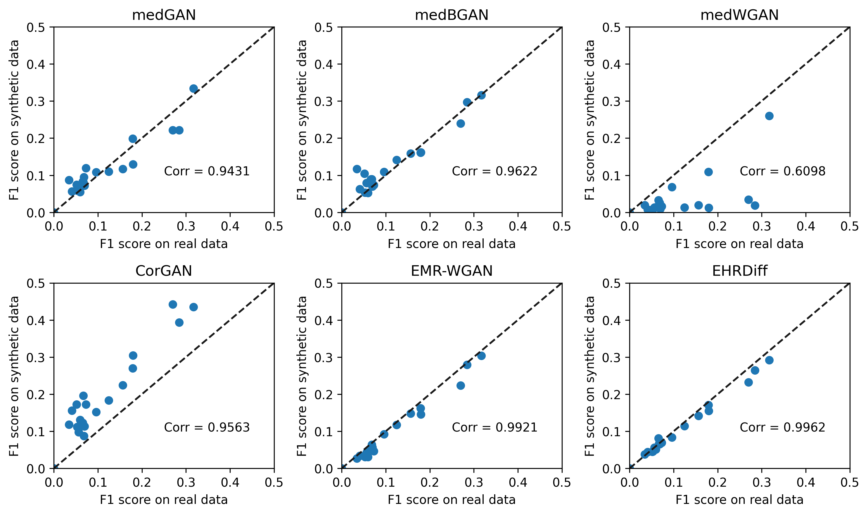
Figure 2: The dimension-wise prediction scatter plot of synthetic EHR data from different generative models against real EHR data. The diagonal lines represent the perfect match of code prediction between synthetic and real EHR data. Each scatter represents a task.

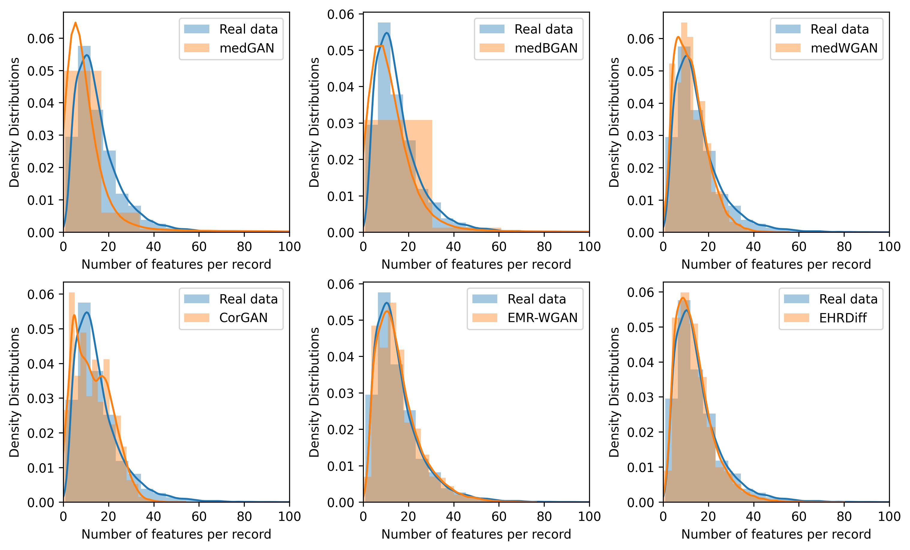
Figure 3: The histograms plot the empirical distributions of the unique code counts on the sample level (bins=20). The solid lines are the kernel density estimations of the distribution.

	APD ($\downarrow$)	NZC ($\uparrow$)	CMD ($\downarrow$)	LD ($\downarrow$)	MCAD ($\downarrow$)
medGAN	1.967	560	29.302	-4.307	0.250
medBGAN	1.406	848	54.833	-4.309	0.112
medWGAN	2.225	420	8.395	-14.761	0.071
CorGAN	2.164	799	11.439	-7.667	0.145
EMR-WGAN	0.511	1039	6.938	-13.881	0.078
EHRDiff	1.256	1677	8.005	-14.487	0.066

Table 1: APD represents Absolute Prevalence Difference, NZC represents Non-Zero code Colunms, CMD represents Correlation Matrix Distance, LD represents Latent Distance, and MCAD represents Medical Concept Abundance Distance. $\downarrow$ and $\uparrow$ indicate the respectively lower and higher numbers for the better results.

	Attribute Inference Risk ($\downarrow$)	Membership Inference Risk ($\downarrow$)
medGAN	0.0009	0.3037
medBGAN	0.0050	0.3036
medWGAN	0.0058	0.2967
CorGAN	0.0023	0.2393
EMR-WGAN	0.0405	0.3139
EHRDiff	0.0129	0.2962

Table 2: The privacy assessment for each model. $\downarrow$ indicates the lower numbers for the better results.

4.5 Results

4.5.1 Utility Results

Figure 1 depicts the dimension-wise prevalence distribution of synthetic EHR data against real data. The scatters from EHRDiff are distributed more closely to the diagonal dashed line compared to other baseline models, and EHRDiff and EMR-WGAN achieve near-perfect correlation values. As shown in Table 1, although EHRDiff lags behind EMR-WGAN in terms of APD, EHRDiff outperforms all baseline methods in NZC by large margins. This shows that APD can be biased by the high prevalence codes and GAN-style baselines all suffer from model collapse to different extents. The results above demonstrate that EHRDiff can better capture the code feature distribution of the real data than the GAN-style baselines. The results above demonstrate that EHRDiff can better capture the overall code prevalence distributions of the real EHR data than the GAN-style baselines and is free from mode collapse.

From CMD results in Table 1, EHRDiff surpasses most baseline models. As shown in Figure 2, the scatters of EHRDiff are closer to the diagonal lines, and achieve the highest correlation value. This means that compared to baselines, the 30 F1 scores of logistic models trained on respectively real and synthetic EHR data are more correlated when evaluated on the same held-out evaluation EHR data. The results demonstrate that EHRDiff can better capture the inherent code feature relation of real EHR data.

From Table 1, it is shown that EHRDiff performs better than most baselines and only marginally falls behind medWGAN by 0.274. In terms of MCAD, EHRDiff consistently outperforms all baselines, and as depicted in Figure 3, we can see that the histogram of unique code count distribution of EHRDiff fits the histogram from real data most. Both metrics demonstrate that the sample-level distribution of the synthetic EHR from EHRDiff resembles that of the real EHR most.

Overall, from the data utility perspective, we can conclude that synthetic EHR data generated by EHRDiff is more realistic and of higher quality compared with baselines. EHRDiff is capable of capturing the real EHR data distribution.

4.5.2 Privacy Results

In Table 2, we list the results on privacy concerns. In terms of attribute inference risk and membership inference risk, EHRDiff achieves middling results. The best results on attribute inference risk and membership inference risk are achieved by medGAN and CorGAN respectively. However, as shown in utility results, the synthesis quality of both models is far worse than EHRDiff . In an extreme circumstance where a generative model fails to fit the real EHR data distribution, the model may achieve perfect results on both privacy metrics. We conjecture that medGAN and CorGAN can better preserve privacy due to mediocre synthesis quality. When compared to EMR-WGAN, which has a satisfying EHR synthesis quality as shown previously, EHRDiff surpasses EMR-WGAN on both metrics. To conclude, EHRDiff can preserve the sensitive private information of real EHR training data.

5 Conclusion

In this work, we explore realistic EHR synthesis with diffusion models. We proposed EHRDiff , a diffusion-based model, for EHR synthesis. Through comprehensive experiments, we empirically demonstrate the superior performance in generating high-quality synthetic EHR data from multiple evaluation perspectives, setting new state-of-the-art EHR synthesis methods. In the meanwhile, we also show EHRDiff can preserve the sensitive private information of real EHR training data. The privacy-preserving advantage allows EHRDiff ’s implementation in real-world scenarios.

References

- Sonabend et al. [2020] Sonabend, A.; Lu, J.; Celi, L. A.; Cai, T.; Szolovits, P. Expert-Supervised Reinforcement Learning for Offline Policy Learning and Evaluation. Advances in Neural Information Processing Systems. 2020; pp 18967–18977.
- Yuan and Yu [2021] Yuan, H.; Yu, S. Efficient Symptom Inquiring and Diagnosis via Adaptive Alignment of Reinforcement Learning and Classification. CoRR 2021, abs/2112.00733.
- Huang et al. [2019] Huang, K.; Altosaar, J.; Ranganath, R. ClinicalBERT: Modeling Clinical Notes and Predicting Hospital Readmission. arXiv:1904.05342 2019,
- Johnson et al. [2016] Johnson, A. E. W.; Pollard, T. J.; Shen, L.; wei H. Lehman, L.; Feng, M.; Ghassemi, M. M.; Moody, B.; Szolovits, P.; Celi, L. A.; Mark, R. G. MIMIC-III, a freely accessible critical care database. Scientific Data 2016, 3.
- Johnson et al. [2023] Johnson, A. E. W.; Bulgarelli, L.; Shen, L.; Gayles, A.; Shammout, A.; Horng, S.; Pollard, T. J.; Moody, B.; Gow, B.; wei H. Lehman, L.; Celi, L. A.; Mark, R. G. MIMIC-IV, a freely accessible electronic health record dataset. Scientific Data 2023, 10.
- Hodge et al. [1999] Hodge, J. G., Jr; Gostin, L. O.; Jacobson, P. D. Legal Issues Concerning Electronic Health InformationPrivacy, Quality, and Liability. JAMA 1999, 282, 1466–1471.
- Choi et al. [2017] Choi, E.; Biswal, S.; Malin, B.; Duke, J.; Stewart, W. F.; Sun, J. Generating Multi-label Discrete Patient Records using Generative Adversarial Networks. Proceedings of the 2nd Machine Learning for Healthcare Conference. 2017; pp 286–305.
- Walonoski et al. [2017] Walonoski, J.; Kramer, M.; Nichols, J.; Quina, A.; Moesel, C.; Hall, D.; Duffett, C.; Dube, K.; Gallagher, T.; McLachlan, S. Synthea: An approach, method, and software mechanism for generating synthetic patients and the synthetic electronic health care record. Journal of the American Medical Informatics Association 2017, 25, 230–238.
- Vincent et al. [2008] Vincent, P.; Larochelle, H.; Bengio, Y.; Manzagol, P.-A. Extracting and Composing Robust Features with Denoising Autoencoders. Proceedings of the 25th International Conference on Machine Learning. New York, NY, USA, 2008; p 1096–1103.
- Biswal et al. [2020] Biswal, S.; Ghosh, S. S.; Duke, J. D.; Malin, B. A.; Stewart, W. F.; Sun, J. EVA: Generating Longitudinal Electronic Health Records Using Conditional Variational Autoencoders. ArXiv 2020, abs/2012.10020.
- Goodfellow et al. [2014] Goodfellow, I.; Pouget-Abadie, J.; Mirza, M.; Xu, B.; Warde-Farley, D.; Ozair, S.; Courville, A.; Bengio, Y. Generative Adversarial Nets. Advances in Neural Information Processing Systems. 2014.
- Baowaly et al. [2018] Baowaly, M. K.; Lin, C.-C.; Liu, C.-L.; Chen, K.-T. Synthesizing electronic health records using improved generative adversarial networks. Journal of the American Medical Informatics Association 2018, 26, 228–241.
- Zhang et al. [2019] Zhang, Z.; Yan, C.; Mesa, D. A.; Sun, J.; Malin, B. A. Ensuring electronic medical record simulation through better training, modeling, and evaluation. Journal of the American Medical Informatics Association 2019, 27, 99–108.
- Yan et al. [2020] Yan, C.; Zhang, Z.; Nyemba, S.; Malin, B. A. Generating Electronic Health Records with Multiple Data Types and Constraints. AMIA Annual Symposium proceedings. AMIA Symposium 2020, 2020, 1335–1344.
- Sohl-Dickstein et al. [2015] Sohl-Dickstein, J.; Weiss, E.; Maheswaranathan, N.; Ganguli, S. Deep Unsupervised Learning using Nonequilibrium Thermodynamics. Proceedings of the 32nd International Conference on Machine Learning. Lille, France, 2015; pp 2256–2265.
- Song et al. [2021] Song, J.; Meng, C.; Ermon, S. Denoising Diffusion Implicit Models. International Conference on Learning Representations. 2021.
- Song et al. [2021] Song, Y.; Sohl-Dickstein, J.; Kingma, D. P.; Kumar, A.; Ermon, S.; Poole, B. Score-Based Generative Modeling through Stochastic Differential Equations. International Conference on Learning Representations. 2021.
- Kong et al. [2021] Kong, Z.; Ping, W.; Huang, J.; Zhao, K.; Catanzaro, B. DiffWave: A Versatile Diffusion Model for Audio Synthesis. International Conference on Learning Representations. 2021.
- Li et al. [2022] Li, X. L.; Thickstun, J.; Gulrajani, I.; Liang, P.; Hashimoto, T. Diffusion-LM Improves Controllable Text Generation. Advances in Neural Information Processing Systems. 2022.
- Yuan et al. [2022] Yuan, H.; Yuan, Z.; Tan, C.; Huang, F.; Huang, S. SeqDiffuSeq: Text Diffusion with Encoder-Decoder Transformers. ArXiv 2022, abs/2212.10325.
- Buczak et al. [2010] Buczak, A. L.; Babin, S.; Moniz, L. J. Data-driven approach for creating synthetic electronic medical records. BMC Medical Informatics and Decision Making 2010, 10, 59 – 59.
- Ghosheh et al. [2022] Ghosheh, G. O.; Li, J.; Zhu, T. A review of Generative Adversarial Networks for Electronic Health Records: applications, evaluation measures and data sources. ArXiv 2022, abs/2203.07018.
- Torfi and Fox [2020] Torfi, A.; Fox, E. A. CorGAN: Correlation-Capturing Convolutional Generative Adversarial Networks for Generating Synthetic Healthcare Records. The Florida AI Research Society. 2020.
- Thanh-Tung et al. [2018] Thanh-Tung, H.; Tran, T.; Venkatesh, S. On catastrophic forgetting and mode collapse in Generative Adversarial Networks. ArXiv 2018, abs/1807.04015.
- Zhang et al. [2020] Zhang, Z.; Yan, C.; Lasko, T. A.; Sun, J.; Malin, B. A. SynTEG: a framework for temporal structured electronic health data simulation. Journal of the American Medical Informatics Association : JAMIA 2020,
- Wang and Sun [2022] Wang, Z.; Sun, J. PromptEHR: Conditional Electronic Healthcare Records Generation with Prompt Learning. Conference on Empirical Methods in Natural Language Processing. 2022.
- He et al. [2023] He, H.; Zhao, S.; Xi, Y.; Ho, J. C. MedDiff: Generating Electronic Health Records using Accelerated Denoising Diffusion Model. 2023; https://arxiv.org/abs/2302.04355.
- Karras et al. [2022] Karras, T.; Aittala, M.; Aila, T.; Laine, S. Elucidating the Design Space of Diffusion-Based Generative Models. Proc. NeurIPS. 2022.
- Hjelm et al. [2018] Hjelm, R. D.; Jacob, A. P.; Trischler, A.; Che, G.; Cho, K.; Bengio, Y. Boundary Seeking GANs. International Conference on Learning Representations. 2018.
- Adler and Lunz [2018] Adler, J.; Lunz, S. Banach Wasserstein GAN. Advances in Neural Information Processing Systems. 2018.
- Torfi and Fox [2020] Torfi, A.; Fox, E. A. CorGAN: Correlation-capturing convolutional generative adversarial networks for generating synthetic healthcare records. arXiv preprint arXiv:2001.09346 2020,
- Zhang et al. [2020] Zhang, Z.; Yan, C.; Mesa, D. A.; Sun, J.; Malin, B. A. Ensuring electronic medical record simulation through better training, modeling, and evaluation. Journal of the American Medical Informatics Association 2020, 27, 99–108.
- Ioffe and Szegedy [2015] Ioffe, S.; Szegedy, C. Batch Normalization: Accelerating Deep Network Training by Reducing Internal Covariate Shift. Proceedings of the 32nd International Conference on Machine Learning. Lille, France, 2015; pp 448–456.
- Ba et al. [2016] Ba, J. L.; Kiros, J. R.; Hinton, G. E. Layer Normalization. 2016; https://arxiv.org/abs/1607.06450.
- Yan et al. [2022] Yan, C.; Yan, Y.; Wan, Z.; Zhang, Z.; Omberg, L.; Guinney, J.; Mooney, S. D.; Malin, B. A. A Multifaceted benchmarking of synthetic electronic health record generation models. Nature Communications 2022, 13.
- Yuan and Yang [2019] Yuan, C.; Yang, H. Research on K-value selection method of K-means clustering algorithm. J 2019, 2, 226–235.
- Agarap [2018] Agarap, A. F. Deep Learning using Rectified Linear Units (ReLU). 2018; https://arxiv.org/abs/1803.08375.