Efficient Real Time Recurrent Learning through combined activity and parameter sparsity

Abstract

Backpropagation through time (BPTT) is the standard algorithm for training recurrent neural networks (RNNs), which requires separate simulation phases for the forward and backward passes for inference and learning, respectively. Moreover, BPTT requires storing the complete history of network states between phases, with memory consumption growing proportional to the input sequence length. This makes BPTT unsuited for online learning and presents a challenge for implementation on low-resource real-time systems. Real-Time Recurrent Learning (RTRL) allows online learning, and the growth of required memory is independent of sequence length. However, RTRL suffers from exceptionally high computational costs that grow proportional to the fourth power of the state size, making RTRL computationally intractable for all but the smallest of networks. In this work, we show that recurrent networks exhibiting high activity sparsity can reduce the computational cost of RTRL. Moreover, combining activity and parameter sparsity can lead to significant enough savings in computational and memory costs to make RTRL practical. Unlike previous work, this improvement in the efficiency of RTRL can be achieved without using any approximations for the learning process.

1 Introduction

Recurrent neural networks are powerful models with a wide variety of applications ranging from language modelling [Merity et al., 2017] to reinforcement learning [Espeholt et al., 2018]. Transformers have supplanted RNNs in many areas of task performance but are impractical for training or inference in resource-constrained environments due to their computational and memory requirements. RNNs may provide a viable alternative, but the most commonly used training algorithm, backpropagation through time (BPTT), requires memory that grows with the length of sequences and does not allow for online updates. Real-time recurrent learning (RTRL) allows for online updates. Memory requirements are independent of sequence length, but the computational requirements are extremely high. This makes it impractical for larger networks – even for a network with 100 units, each step would require on the order of $10^{6}$ computations.

Event-based neural networks (EvNNs) with activity sparsity have been previously proposed to make RNNs more efficient and include spiking neural networks [Maass, 1997] and the EGRU [Subramoney et al., 2022] among others. For the EGRU, which is a form of EvNN based on GRU dynamics, Subramoney et al. [2022] show that an EvNN with activity sparsity requires fewer operations not only for inference but also during training with BPTT. However, due to the disadvantages of BPTT listed above, we explore using RTRL for these EvNNs. We show that for EvNNs with activity sparsity, the computational requirements of RTRL can be reduced to be proportional to $\tilde{\beta}^{2}n^{2}p$ (rather than $n^{2}p$ for dense RTRL) where $\beta=1-\tilde{\beta}$ is the sparsity of the derivative of the activations of the units in the backward pass. The memory requirement is also reduced by a factor of $\tilde{\beta}$. Moreover, we show that benefits due to activity sparsity compose well with those with parameter sparsity. With the combination of the two sparsities, the computational cost is ameliorated significantly to be proportional to $\tilde{\omega}^{2}\tilde{\beta}^{2}n^{2}p$ (rather than $n^{2}p$ for dense RTRL) where $\omega=1-\tilde{\omega}$ is the parameter sparsity, $n$ is the size of the network state, and $p$ is the number of parameters ($p=n^{2}$ for a fully connected vanilla RNN). Since $\tilde{\beta}$ and $\tilde{\omega}$ are value between 0 and 1, the savings in compute cost can be significant. Subramoney et al. [2022] demonstrate that the EGRU achieves about 50% backward sparsity in most of their experiments. With just activity sparsity, this translates to a multiplier of $\tilde{\beta}^{2}=(1-0.5)^{2}=0.25$ or 25% of the operations required for dense RTRL without activity sparsity. Combined with parameter sparsity of  80%, the multiplier is $0.2^{2}0.5^{2}=0.01$, which translates to 1% of operations required for dense RTRL. This is achieved without the need for approximating the RTRL updates.

The benefits of these computational savings can be realised to the fullest extent on devices with support for unstructured sparsity. Support for unstructured sparsity has been increasing both on established hardware types such as GPUs [Pool et al., 2021] and newer hardware designed for deep learning [Jia et al., 2019, Lewington, 2021] as well as neuromorphic devices [Davies et al., 2018, Höppner et al., 2017].

2 Related work

There is a long line of work exploring methods to make RTRL more efficient – see Marschall et al. [2020] for an extensive review. But most previous approaches have involved finding good approximations for calculating the influence matrix in RTRL. We use the canonical, exact equations for calculating the RTRL influence matrix while taking advantage of the natural computational advantage that arises from having an activity-sparse network such as the EvNN/EGRU. Menick et al. [2020] have explored the influence of parameter sparsity in making RTRL more efficient and conclude that by itself, the gains are limited due to the form of interactions between parameters and activations in recurrent networks. They propose approximations combined with parameter sparsity that can lead to computationally more efficient RTRL, whereas we use the exact form of RTRL updates to achieve computational efficiency.

3 Real Time Recurrent Learning

Method		memory	time per step
Fully dense	BPTT	$Tn+p$	$n^{2}+p$
	RTRL	$n+np$	$n^{2}+n^{2}p$
Sparse RTRL	with parameter sparsity	$n+\tilde{\omega}np$	$\tilde{\omega}n^{2}+\tilde{\omega}^{2}n^{2}p$
	with activity sparsity	$\tilde{\alpha}n+\tilde{\beta}np$	$\tilde{\alpha}n^{2}+\tilde{\beta}^{2}n^{2}p$
	with both	$\tilde{\alpha}n+\tilde{\omega}\tilde{\beta}np$	$\tilde{\omega}\tilde{\alpha}n^{2}+\tilde{\omega}^{2}\tilde{\beta}^{2}n^{2}p$
Approximate RTRL	SnAp-1 [Menick et al., 2020]	$n+\tilde{\omega}p$	$\tilde{\omega}n^{2}+\tilde{\omega}p$
	SnAp-2 [Menick et al., 2020]	$n+\tilde{\omega}^{2}np$	$\tilde{\omega}n^{2}+\tilde{\omega}^{3}n^{2}p$

Table 1: Computational and memory costs for sparse and dense methods, including approximations. $T$ refers to sequence length, $n$ the number of hidden units, $p$ the number of dense parameters. $\omega=1-\tilde{\omega}$ is the level of parameter sparsity, $\alpha=1-\tilde{\alpha}$ is the level of activity sparsity in the forward pass, and $\beta=1-\tilde{\beta}$ is the level of sparsity in the derivative of activation (see text for further explanation). The first term of each compute cost is for the forward pass, and the second term is for updating the influence matrix.

Following the notation in [Marschall et al., 2020], we define a recurrent network that has a state $\mathbf{a}^{(t)}\in\mathbb{R}^{n}$ at each timestep $t$. This state is updated with function $F:\mathbb{R}^{m}\rightarrow\mathbb{R}^{n}$ parameterised by the flattened recurrent parameter vector $\mathbf{w}\in\mathbb{R}^{p}$, and input parameter vector $\mathbf{w}_{\text{in}}\in\mathbb{R}^{n_{\text{in}}}$. Here $m=n+n_{\text{in}}+1$ is the total number of input dimensions, $n$ being the number of hidden units, $n_{\text{in}}$ the dimensionality of the input, and the $+1$ to include a bias term. For a densely connected vanilla RNN $p=n^{2}$. We first consider activity sparsity and derive the computational savings for a fully connected vanilla RNN (the derivation is equivalent for architectures such as the GRU or EGRU).

Consider a network whose dynamics is defined by

$$\mathbf{a}^{(t)}=F\left(\mathbf{a}^{(t-1)},\;\mathbf{x}^{(t)};\mathbf{w}\right).$$ (1)

An output $\mathbf{y}^{(t)}\in\mathbb{R}^{n_{\text{out}}}$ is computed at every timestep using a readout function $\mathbf{y}^{(t)}=F_{\text{out}}\left(\mathbf{a}^{(t)};\mathbf{w}_{o}\right)$, where $\mathbf{w}_{o}$ are the readout parameters. This output determines the instantaneous loss at every time step, calculated as $L^{(t)}=L\left(\mathbf{y}^{(t)},\;\mathbf{y}_{\text{target}}^{(t)}\right)$, where $L$ is some loss function, say MSE or cross-entropy loss. The goal of training is to minimize the total loss over all timesteps $\mathcal{L}=\sum_{t}L^{(t)}$ using gradient descent on all the parameters.

For updating the recurrent parameters, we need to calculate $\frac{\partial\mathcal{L}}{\partial\mathbf{w}}$. We consider how this quantity can be calculated using RTRL, starting with

$$\frac{\partial\mathcal{L}}{\partial\mathbf{w}}=\sum_{t=0}^{T}\frac{\partial L^{(t)}}{\partial\mathbf{w}}=\sum_{t}\sum_{s=0}^{t}\frac{\partial L^{(t)}}{\partial\mathbf{w}^{(s)}},$$ (2)

where $\mathbf{w}^{(s)}$ refers to the application of the parameters $\mathbf{w}$ at timestep $s$ (equivalent to the partial derivative of $L^{(t)}$). Using chain rule, this can be written as

$$\frac{\partial L^{(t)}}{\partial\mathbf{w}}=\left(\frac{\partial\mathbf{a}^{(t)}}{\partial\mathbf{w}}\right)^{T}\frac{\partial L^{(t)}}{\partial\mathbf{a}^{(t)}}\equiv\left(\mathbf{M}^{(t)}\right)^{T}\bar{\mathbf{c}}^{(t)},$$ (3)

where $.^{T}$ refers to matrix transpose. We refer to $\mathbf{M}^{(t)}=\partial\mathbf{a}^{(t)}/\partial\mathbf{w}\in\mathbb{R}^{n\times p}$ as the influence matrix, and $\bar{\mathbf{c}}^{(t)}=\partial L^{(t)}/\partial\mathbf{a}^{(t)}\in\mathbb{R}^{n}$ as the credit assignment vector.

In RTRL, $\mathbf{M}^{(t)}$ is defined by the following recursive relationship:

$$\mathbf{M}^{(t)}\equiv\mathbf{J}^{(t)}\mathbf{M}^{(t-1)}+\bar{\mathbf{M}}^{(t)},$$ (4)

where the jacobian $\mathbf{J}^{(t)}=\partial\mathbf{a}^{(t)}/\partial\mathbf{a}^{(t-1)}\in\mathbb{R}^{n\times n}$ and the immediate influence matrix $\bar{\mathbf{M}}^{(t)}=\partial\mathbf{a}^{(t)}/\partial\mathbf{w}^{(t)}\in\mathbb{R}^{n\times p}$ are used.

The main computational cost of RTRL arises from having to multiply $\mathbf{J}^{(t)}$ and $\mathbf{M}^{(t-1)}$, which are $n\times n$ and $n\times p$ matrices respectively, which requires $\mathcal{O}(n^{2}p)$ computations. Moreover, we need to store $\mathbf{M}^{(t)}$ at every step, requiring $\mathcal{O}(np)$ memory. For a fully connected vanilla RNN, $p=n^{2}$, requiring $\mathcal{O}(n^{4})$ computations and $\mathcal{O}(n^{3})$ memory.

4 Efficient RTRL with activity sparsity

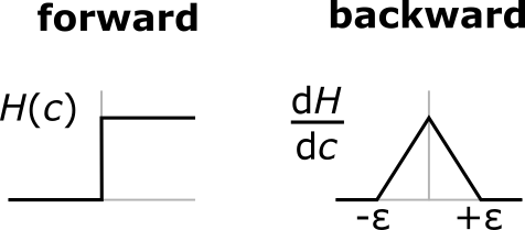
Figure 1: Illustration of surrogate gradient (pseudo-derivative)

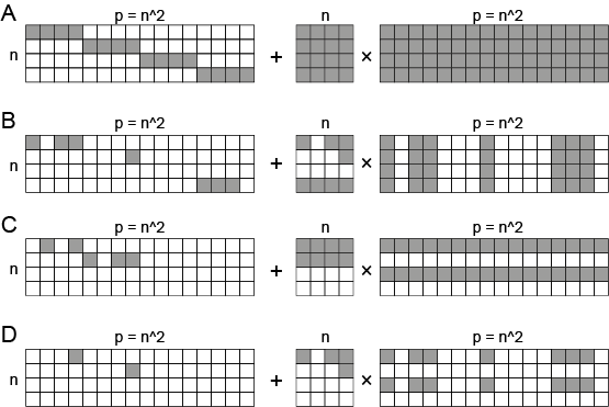
Figure 2: Illustration of RTRL updates with various types of sparsity. (A) Dense network. (B) With only parameter sparsity. (C) With only activity sparsity. (D) With both activity and parameter sparsity.

We now show how activity sparsity can ameliorate these computational and memory requirements. Any network with an activation function and derivative that induces sparsity, and with the appropriate dynamics can potentially benefit from computational and memory savings. For simplicity, we focus on showing this for a network based on the EGRU [Subramoney et al., 2022] that uses a Heaviside step function with a pseudo-derivative. Specifically, consider a network where the internal state is gated by a threshold function

$$\mathbf{a}^{(t)}=H\left(\mathbf{v}^{(t)}\right),$$ (5)

where $H$ is the Heaviside step function, and $\mathbf{v}^{(t)}=F\left(\mathbf{a}^{(t-1)},\mathbf{x}^{(t)}\right)-\mathbf{\vartheta}$, $\mathbf{\vartheta}$ defined as a vector containing ‘thresholds’ for each unit of the network. As in Subramoney et al. [2022], the gradient of the Heaviside step function is defined using a surrogate function (or pseudo-derivative) to be $H^{\prime}(\mathbf{v}_{k}^{(t)})=\gamma\text{max}\{0,1-\frac{|\mathbf{v}_{k}^{(t)}|}{2\epsilon}\}$, where $\gamma$ defines the height of the pseudo-derivative, and $\epsilon$ defines the width of the pseudo-derivative. See Fig. 2 for an illustration.

At timestep $t$, let $\alpha^{(t)}$ be the activity-sparsity of the network i.e. $\alpha^{(t)}$ fraction of the units have zero activation. For a unit $k$ with zero activation, $\mathbf{a}^{(t)}_{k}=0$ because $\mathbf{v}^{(t)}_{k}\leq 0$. Let $\beta^{(t)}$ be the fraction of the units which have a zero derivative. For a unit $k$ with zero derivative, $H^{\prime}(\mathbf{v}^{(t)}_{k})=0$ because $\mathbf{v}^{(t)}_{k}>\epsilon\text{ or }\mathbf{v}^{(t)}_{k}<-\epsilon$.

Now considering a single element of the Jacobian,

$$\mathbf{J}_{kl}^{(t)}=\frac{\partial\mathbf{a}_{k}^{(t)}}{\partial\mathbf{a}_{l}^{(t-1)}}=H^{\prime}\left(\mathbf{v}_{k}^{(t)}\right)\frac{\partial\mathbf{v}_{k}^{(t)}}{\partial\mathbf{a}_{l}^{(t-1)}},$$ (6)

it is clear that this term is zero for all units $k$ where $\mathbf{v}^{(t)}_{k}>\epsilon\text{ or }\mathbf{v}^{(t)}_{k}<-\epsilon$. This implies that entire rows of the matrix $\mathbf{J}$ are zero, when the unit state $\mathbf{v}_{k}^{(t)}$ lies in that range ($\beta^{(t)}\times n$ rows to be precise).

Similarly, for the immediate influence matrix $\bar{\mathbf{M}}^{(t)}$,

$$\bar{\mathbf{M}}^{(t)}_{kp}=\frac{\partial\mathbf{a}^{(t)}_{k}}{\partial\mathbf{w}^{(t)}_{p}}=H^{\prime}\left(\mathbf{v}^{(t)}_{k}\right)\frac{\partial\mathbf{v}_{k}^{(t)}}{\partial\mathbf{w}^{(t)}_{p}},$$ (7)

all rows corresponding to units whose states $\mathbf{v}_{k}^{(t)}$ lie between $\pm\epsilon$ are zero ($\beta^{(t)}\times n$ rows to be precise). This is in addition to the default sparsity of $\bar{\mathbf{M}}$ since only terms immediately local to each unit are non-zero.

Each recursive update of the influence matrix can be written as

$$\mathbf{M}_{kp}^{(t)} =\sum_{l}\mathbf{J}_{kl}^{(t)}\mathbf{M}_{lp}^{(t-1)}+\bar{\mathbf{M}}_{kp}^{(t)},$$ (8)

$$=\sum_{l}H^{\prime}\left(\mathbf{v}_{k}^{(t)}\right)\frac{\partial\mathbf{v}_{k}^{(t)}}{\partial\mathbf{a}_{l}^{(t-1)}}\mathbf{M}_{lp}^{(t-1)}+H^{\prime}\left(\mathbf{v}^{(t)}_{k}\right)\frac{\partial\mathbf{v}_{k}^{(t)}}{\partial\mathbf{w}^{(t)}_{p}}$$ (9)

$$=H^{\prime}\left(\mathbf{v}^{(t)}_{k}\right)\left[\sum_{l}\frac{\partial\mathbf{v}_{k}^{(t)}}{\partial\mathbf{a}_{l}^{(t-1)}}\mathbf{M}_{lp}^{(t-1)}+\frac{\partial\mathbf{v}_{k}^{(t)}}{\partial\mathbf{w}^{(t)}_{p}}\right].$$ (10)

This implies that at each timestep $t$, $\beta^{(t)}\times n$ rows of the matrix $\mathbf{M}^{(t)}$ are fully $0$.

Taken together with Eqns. (6), (7), at each time $t$, $\mathbf{J}^{(t)}$ has $\beta^{(t)}$ fraction of rows zero, and $\mathbf{M}^{(t-1)}$ has $\beta^{(t-1)}$ fraction of rows zero. Defining $\tilde{\beta}^{(t)}=1-\beta^{(t)}$ and $\tilde{\beta}^{(t-1)}=1-\beta^{(t-1)}$, the matrix multiplication is on the order of $\mathcal{O}(\tilde{\beta}^{(t)}n\times\tilde{\beta}^{(t-1)}n\times p)=\mathcal{O}(\tilde{\beta}^{(t-1)}\tilde{\beta}^{(t)}n^{2}p)$. And at each timestep $t$, we would require $\mathcal{O}(\tilde{\beta}^{(t)}n\times p)=\mathcal{O}(\tilde{\beta}^{(t)}np)$ storage.

5 Efficient RTRL with activity AND parameter sparsity

As described in Menick et al. [2020], for recurrent networks in the form of a vanilla RNN or GRU (and by extension EGRU), parameter sparsity introduces sparsity in elements of $\mathbf{J}$, and sets entire columns of $\bar{\mathbf{M}}$ to zero. If the parameter sparsity pattern is fixed, then corresponding columns of $\mathbf{M}$ remain zero across timesteps as well. Therefore, with a parameter sparsity of $\omega=1-\tilde{\omega}$, and activity sparsity, the compute requirement for the influence matrix updates from Eq. (4) is $\mathcal{O}(\tilde{\beta}^{(t)}n\times\tilde{\omega}\tilde{\beta}^{(t-1)}n\times\tilde{\omega}p)=\mathcal{O}(\tilde{\beta}^{(t)}\tilde{\beta}^{(t-1)}\tilde{\omega}^{2}n^{2}p)$. The memory requirement for storing the influence matrix is $\mathcal{O}(\tilde{\beta}^{(t)}n\times\tilde{\omega}p)=\mathcal{O}(\tilde{\beta}^{(t)}\tilde{\omega}np)$.

Fig. 2 demonstrates various different cases without and with activity and parameter sparsity. The sparsity of the influence matrix due to activity sparsity depends on the sparsity of the derivative of the activation function. And in this case, corresponding rows of $\mathbf{J}$ and $\mathbf{M}$ and $\bar{\mathbf{M}}$ become zeros when the derivative of the activation function becomes zero for a neuron. In the case of parameter sparsity, elements of $\mathbf{J}$ and columns of $\mathbf{M}$ and $\bar{\mathbf{M}}$ become zero when a parameter is zero. See Table 1 for the full comparison.

6 Results

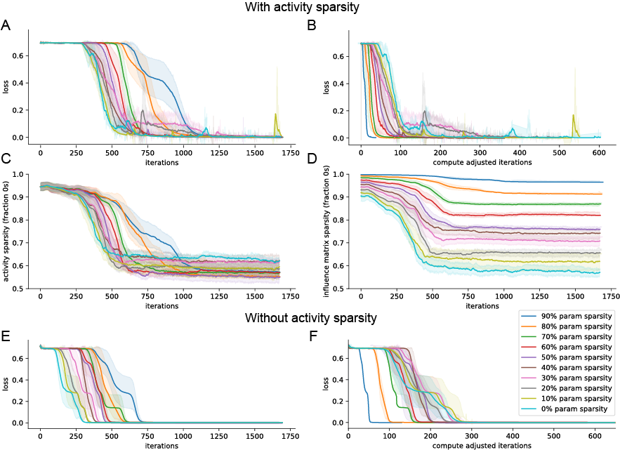
Figure 3: Computational savings and sparsity results on synthetic dataset. Mean and std err over 5 runs.

We use RTRL with combined activity and parameter sparsity on a synthetic classification task where a two-dimensional spiral unwinding over time is classified as clockwise or anti-clockwise. The dataset consisted of 10,000 randomly generated spirals of 17 timesteps length assigned to one of the two classes depending on the orientation of the spiral. We trained an EGRU [Subramoney et al., 2022] with 16 hidden units for 1700 iterations with Adam [Kingma and Ba, 2015] and a batch size of 32. Note that most variants converge well before 1700 iterations. For cases where the parameter sparsity was non-zero, we chose a fixed random sparsity mask at initialisation and trained the network with this sparsity mask throughout.

The learning curves of a network with activity sparsity and various levels of parameter sparsity are shown in Fig. 3A. Those for the case without activity sparsity are shown in Fig. 3E. The x axis here shows the number of iterations/epochs corresponding to parameter updates. We consider a measure of total compute with the compute adjusted iteration, defined as the cumulative sum of the computational savings factor $\tilde{\omega}^{2}\tilde{\beta}^{2}$ (or $\tilde{\omega}^{2}$). Note that the compute adjusted iteration is an analytical measure for the total compute used in an optimal case where the underlying hardware architecture is optimised for the algorithm, and does not take memory access and computational bottlenecks into consideration. Using this measure, we can see in Figs. 3B and F that the combination of high (90%) parameter sparsity with activity sparsity converges with the least total compute. Figs. 3C and D show the activity and influence matrix sparsity respectively for different degrees of parameter sparsity for a network with activity sparsity enabled. Since the parameter sparsity is fixed at initialisation does not change, the influence matrix sparsity also remains fixed throughout training when activity sparsity is turned off.

7 Discussion

We demonstrate the advantage of combining activity and parameter sparsity both analytically and empirically on a small synthetic dataset. We demonstrate the result on an event-based network architecture (EGRU [Subramoney et al., 2022]) that is naturally activity sparse. Even with modest levels of activity and parameter sparsity, the computational savings realisable in RTRL is quite significant, making RTRL potentially applicable to real world tasks. While we use fixed parameter sparsity, methods such as [Bellec et al., 2018] allow for optimising the parameter sparsity pattern during training.

In order to fully realise the compute savings, an optimised implementation that runs on hardware supporting unstructured sparsity is required. With the two forms of sparsity considered here, a message-passing implementation of RTRL can provide a new practical event-based way of training recurrent neural networks on neuromorphic devices as well. On the whole, given the appropriate hardware substrate, RTRL with a combination of activity and parameter sparsity can provide a practical and competitive alternative to BPTT.

8 Acknowledgements

We acknowledge the use of Fenix Infrastructure resources, which are partially funded from the European Union’s Horizon 2020 research and innovation programme through the ICEI project under the grant agreement No. 800858. AS was funded by the Ministry of Culture and Science of the State of North Rhine-Westphalia, Germany during this work. AS would like to thank Mark Schöne, Khaleelulla Khan Nazeer and David Kappel for helpful discussions and comments on this manuscript, and Laurenz Wiskott for institutional support.

References

- Bellec et al. [2018] G. Bellec, D. Kappel, W. Maass, and R. Legenstein. Deep Rewiring: Training very sparse deep networks. In International Conference on Learning Representations, Feb. 2018. URL https://openreview.net/forum?id=BJ_wN01C-.
- Davies et al. [2018] M. Davies, N. Srinivasa, T.-H. Lin, G. Chinya, Y. Cao, S. H. Choday, G. Dimou, P. Joshi, N. Imam, S. Jain, et al. Loihi: A neuromorphic manycore processor with on-chip learning. Ieee Micro, 38(1):82–99, 2018.
- Espeholt et al. [2018] L. Espeholt, H. Soyer, R. Munos, K. Simonyan, V. Mnih, T. Ward, Y. Doron, V. Firoiu, T. Harley, I. Dunning, S. Legg, and K. Kavukcuoglu. IMPALA: Scalable Distributed Deep-RL with Importance Weighted Actor-Learner Architectures. arXiv:1802.01561 [cs], Feb. 2018. URL http://arxiv.org/abs/1802.01561.
- Höppner et al. [2017] S. Höppner, Y. Yan, B. Vogginger, A. Dixius, J. Partzsch, F. Neumärker, S. Hartmann, S. Schiefer, S. Scholze, G. Ellguth, et al. Dynamic voltage and frequency scaling for neuromorphic many-core systems. In 2017 IEEE International Symposium on Circuits and Systems (ISCAS), pages 1–4. IEEE, 2017.
- Jia et al. [2019] Z. Jia, B. Tillman, M. Maggioni, and D. P. Scarpazza. Dissecting the graphcore ipu architecture via microbenchmarking. arXiv preprint arXiv:1912.03413, 2019.
- Kingma and Ba [2015] D. P. Kingma and J. Ba. Adam: A method for stochastic optimization. In Y. Bengio and Y. LeCun, editors, 3rd International Conference on Learning Representations, ICLR 2015, San Diego, CA, USA, May 7-9, 2015, Conference Track Proceedings, 2015. URL http://arxiv.org/abs/1412.6980.
- Lewington [2021] R. Lewington. Cerebras systems: Achieving industry best ai performance through a systems approach. https://8968533.fs1.hubspotusercontent-na1.net/hubfs/8968533/Whitepapers/Cerebras-CS-2-Whitepaper.pdf, 2021. [Online; accessed 07-Feb-2023].
- Maass [1997] W. Maass. Networks of spiking neurons: the third generation of neural network models. Neural networks, 10(9):1659–1671, 1997.
- Marschall et al. [2020] O. Marschall, K. Cho, and C. Savin. A Unified Framework of Online Learning Algorithms for Training Recurrent Neural Networks. Journal of Machine Learning Research, 21(135):1–34, 2020. ISSN 1533-7928. URL http://jmlr.org/papers/v21/19-562.html.
- Menick et al. [2020] J. Menick, E. Elsen, U. Evci, S. Osindero, K. Simonyan, and A. Graves. Practical Real Time Recurrent Learning with a Sparse Approximation. In International Conference on Learning Representations, Sept. 2020. URL https://openreview.net/forum?id=q3KSThy2GwB.
- Merity et al. [2017] S. Merity, N. S. Keskar, and R. Socher. Regularizing and Optimizing LSTM Language Models. arXiv:1708.02182 [cs], Aug. 2017.
- Pool et al. [2021] J. Pool, A. Sawarkar, and J. Rodge. Accelerating Inference with Sparsity Using the NVIDIA Ampere Architecture and NVIDIA TensorRT. https://developer.nvidia.com/blog/accelerating-inference-with-sparsity-using-ampere-and-tensorrt/, 2021. [Online; accessed 07-Feb-2023].
- Subramoney et al. [2022] A. Subramoney, K. K. Nazeer, M. Schöne, C. Mayr, and D. Kappel. EGRU: Event-based GRU for activity-sparse inference and learning, June 2022. URL http://arxiv.org/abs/2206.06178.