Self-Supervised One-Shot Learning for Automatic Segmentation of StyleGAN Images

Abstract

We propose a framework for the automatic one-shot segmentation of synthetic images generated by a StyleGAN. Our framework is based on the observation that the multi-scale hidden features in the GAN generator hold useful semantic information that can be utilized for automatic on-the-fly segmentation of the generated images. Using these features, our framework learns to segment synthetic images using a self-supervised contrastive clustering algorithm that projects the hidden features into a compact space for per-pixel classification. This contrastive learner is based on using a novel data augmentation strategy and a pixel-wise swapped prediction loss that leads to faster learning of the feature vectors for one-shot segmentation. We have tested our implementation on five standard benchmarks to yield a segmentation performance that not only outperforms the semi-supervised baselines by an average wIoU margin of $1.02\%$ but also improves the inference speeds by a factor of $4.5$. Finally, we also show the results of using the proposed one-shot learner in implementing BagGAN, a framework for producing annotated synthetic baggage X-ray scans for threat detection. This framework was trained and tested on the PIDRay baggage benchmark to yield a performance comparable to its baseline segmenter based on manual annotations.

1 Introduction

Generative Adversarial Networks or GANs [20] have consistently defined the state-of-the-art in generative modeling of image data for synthesizing photo-realistic images for several applications. Style-based implementations of GANs have not only enabled the synthesis of high fidelity, high resolution images but also paved the way to learning disentangled latent representations that can control semantic attributes in the generated images [26, 25, 27].

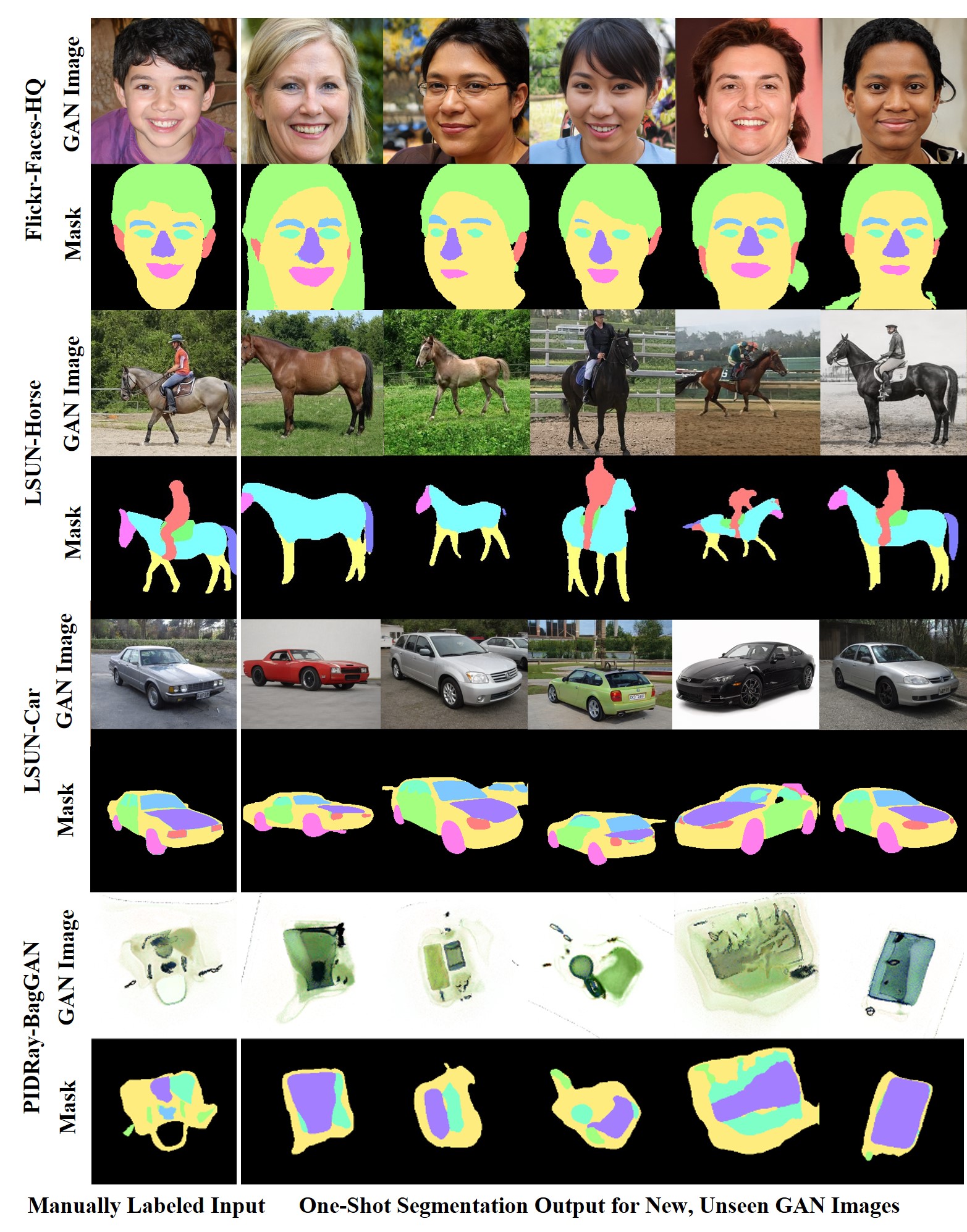
Figure 1: Results of one-shot segmentation with our proposed framework on different datasets: For each of the four example illustrations, the first column denotes the manually labeled input sample to our one-shot segmenter while the other columns denote the segmenter outputs produced for new unseen images. The first three illustrations show the results for the FF-HQ [26], LSUN-Horse and LSUN-Car [47] datasets respectively, while the last illustration shows the results for our BagGAN framework for generating synthetic X-ray baggage scans. For the BagGAN case, the StyleGAN model was pre-trained on the PIDRay dataset [43].

The data generated using GANs, however, does not lend itself to being directly used in supervised learning applications without first being curated through annotations. For segmentation tasks, the pixel-wise annotation of images can be costly and time-consuming for both real and synthetic images alike. A number of works have therefore investigated the problem of automatic extraction of segmentation labels from synthetic images generated using GANs [51, 31, 42, 45]. Section 2 presents a review of these methods.

As pointed out in Y. Zhang . [51], what makes the case of GAN-generated images special in this regard is the fact that a GAN has already learned the latent feature representations at different scales of the generated image when it is trained to map a lower dimensional latent vector to a full-scale image. These learned feature representations, which are extracted from the style block activations of a GAN during image synthesis, can be used to predict the semantic properties of the generated pixels. For example, Yang . [44] and Pakhomov . [37] have demonstrated the use of these feature representations for unsupervised data clustering with GANs.

In this paper, we further explore the properties of these GAN-generated feature representations for the self-supervised learning [24] of what it takes to automatically segment the images into semantically meaningful components as they are being generated by the GAN. For carrying out such automatic segmentation we employ one-shot learning wherein only a single sample is required to specify the regions of interest to be identified in new unseen images.

To that end, we make use of the aforementioned hidden features obtained from different GAN layers that have been observed to characterize the multi-scale visual properties of images produced by GANs [52]. This feature set is used in our work to implement a framework for on-the-fly, one-shot segmentation of GAN-generated images.

The novelty of our proposed one-shot learning framework lies in the self-supervised clustering model used for feature learning during the segmentation of GAN-generated images. While existing methods like DatasetGAN [51] and RepurposeGAN [42] also use generator hidden features to segment GAN images, our framework introduces an additional self-supervised clustering model to process these features before they are fed to the segmenter. The new feature space learnt by the self-supervised model allows for faster, improved learning for the one-shot segmenter.

To construct this self-supervised model, our starting point is the prior work [39, 1] with extended latent spaces for GANs. These authors have shown that given an extended latent space $W^{+}\{\textbf{w}_{i}|\>i=1,\ldots,L\}$ for a pre-trained StyleGAN, how it is possible to exploit the latent vectors that are fed into the different layers of a StyleGAN to affect meaningful changes at different scales in the output. What’s interesting is that these controlled perturbations to the latent vectors generate exactly the sort of output-image augmentations that are needed for the self-supervised contrastive learning in our framework. To that effect, we have implemented a novel image augmentation strategy based on latent vector perturbations in our proposed work on self-supervised one-shot segmentation.

This work uses a clustering based approach to implement the self-supervised learner for one-shot segmentation. In general, clustering-based methods for self-supervision learn latent representations for unlabeled data through ‘pseudo-label’ assignments obtained from unsupervised data clustering [7, 3] – these pseudo-label assignments serve as intermediate data encodings which can later be fine-tuned for downstream supervised learning tasks.

Our particular contrastive clustering strategy is based on the well-known SwAV (Swapped Assignment between Views) approach [8] in which representational learning is achieved by comparing cluster assignments for a set of images and their augmented counterparts instead of using direct feature comparisons between transformed image pairs. In our implementation, we have applied this approach to the hidden features of a pre-trained StyleGAN. The scalability of the SwAV method allows us to process large batches of pixelwise cluster assignments for image segmentation without having to process every pixel pair. As we will show, using the GAN hidden features in this manner also contributes to more efficient learning that is required for one-shot segmentation. A detailed formulation of our implemented self-supervised algorithm is described in Section 6 along with the implementation results that are presented in Section 7.

We have tested our framework on a number of standard datasets for one-shot segmentation, including the CelebA dataset [34], the LSUN dataset [48] and the PASCAL-Part dataset [48]. The tests were performed by using StyleGAN models which were pre-trained on these datasets and then connecting the one-shot segmenter to the pre-trained generator to process the synthesized image. The segmentation performance of our implementation shows a higher wIOU for one-shot learning compared with the other baseline methods like DatasetGAN [51] and RepurposeGAN [42] especially for low-frequency object labels. Furthermore, a comparison of the inference times reveals a 4.5x faster performance with the implemented models.

We have also used the proposed framework in the implementation of BagGAN, a GAN-based framework for generating annotated synthetic X-ray baggage scans for threat detection. The BagGAN framework is designed to produce realistic X-ray scans of checked baggage using StyleGANs while automatically extracting segmentation labels from the simulated images. This framework was implemented with a StyleGAN pre-trained on the PIDRay baggage screening benchmark [43] and our proposed one-shot segmenter was then applied to the synthesized images to create new annotated samples for different threat items. Testing the framework for 5 different threat categories has yielded an segmentation performance which stands close to the performance of its baseline segmenter based on manual annotations.

The organization of the paper is as follows: Section 2 provides a literature survey on automatic segmentation methods using GANs and the different methods for one-shot learning. Section 3 then describes the concepts and methods used in our proposed framework. This is followed by Section 4 that presents our self-supervised model for hidden feature clustering, followed by Section 5 that describes how automatic one-shot learning for segmentation is carried out over the output of hidden-feature clustering. The results on the datasets used are presented in Section 7 and the results obtained via the BagGAN application of the framework are presented in Section 8. Finally, Section 9 presents the ablation studies.

2 Related Work

2.1 GANs for Image Synthesis

There now exist several different classes of deep generative models [6] that can learn from a domain data distribution and synthesize new data that resembles samples from that distribution. These classes include encoder-decoder architectures such as VAEs [28], generative adversarial networks (GANs) [20], auto-regressive models [4] and the more recently proposed diffusion models [17]. Out of these, the family of generative adversarial networks (GANs) have for a long time remained the dominant technique in synthesizing high quality image datasets for several applications.

Style-based implementations of GANs, which form the current state-of-the-art for these models, not only excel in producing photo-realistic images at scale [26, 25, 27] but have also paved the way for effective disentangled representation learning [21]. The broad goal of representation learning is to enable GANs to learn the latent representations for the different semantic components in the images. This allows for the training of more ‘interpretable’ GANs that can control the semantic attributes of the generated images. A number of works have therefore utilized StyleGANs for applications like semantic image editing [32], guided image generation [40] and image inpainting [14]. In our own work, we have exploited the disentangled latent space, $W^{+}$ of StyleGANs for one-shot learning as discussed in Section 3.

2.2 Automatic Segmentation with GANs

The ability of GANs to create large-scale synthetic image datasets also raises the question of the annotation of these images for supervised learning tasks like semantic segmentation. Several methods have thus been proposed for the automatic extraction of segmentation labels from GAN generated images. These methods broadly fall into the two following categories depending on whether the segmentation is learnt using unsupervised or semi-supervised methods:

2.2.1 Unsupervised Approaches

Unsupervised methods of automatic segmentation use latent feature representations from pretrained GANs to implicitly learn pixel-wise labels for the GAN generated images. Such methods are useful for automatic foreground-background discrimination when a GAN is trained on data samples that portray a distinct object class against diverse backgrounds (Z. Liu . [34] being an example of such a dataset). Works such as Abdal . [2] and Benny  Wolf [5] fall into this category and are mainly applicable for segmentation tasks where the foreground and the background are independent of each other. Other implementations such as Pakhomov . [37] also use unsupervised clustering to partition the image into semantically meaningful regions but still require a contextual encoder to assign labels to the clustered regions.

2.2.2 Semi-Supervised Approaches

Semi-supervised learning involves the combined use of a small set of labeled data with a larger set of unlabeled data to facilitate network training with small labeled datasets. For our problem case, the corpus of unlabeled data is the set of synthetic images generated using GANs for which the network has already learnt the latent feature representations during training. Works like DatasetGAN [51] and SemanticGAN [31] exploit this fact to perform semantic segmentation of GAN generated data using a small set of manually annotated samples. Notably, in DatasetGAN [51], this is done by using hidden feature activations from the GAN to train a style interpreter for semantic segmentation. In our work, we use a similar strategy for one-shot segmentation wherein the hidden features are processed using self-supervised learning as described in the rest of this paper.

2.3 One-Shot Learning for Image Segmentation

One-shot learning refers to a special subset of supervised learning where the training data is limited to only one labeled sample. The problem typically translates into fine-tuning a pre-trained classifier to identify unseen class labels using a small support set of training samples and with the help of the knowledge acquired through pre-training on other class labels. Hence, one-shot learning is practically implemented using either semi-supervised or self-supervised methods. Both these approaches are enumerated for semantic segmentation as follows:

2.3.1 Semi-Supervised Segmentation

Semi-supervised one-shot learners have been implemented for semantic segmentation either by tuning the parameters of a pre-trained network to segment new semantic classes [18] or by using comparison networks for similarity matching between the query and support images [50, 49]. The former approach relies on segmenters that are pre-trained on similar annotation tasks as the support samples while the latter requires training a new comparison network using support-query image pairs. Hence, neither approach can be incorporated in a GAN network that must automatically output a labeled segmentation map for the generated images. In that context, new methods for one-shot segmentation with GANs have been proposed which are inspired from the success of Y. Zhang . [51] in automatic annotation. For example, RepurposeGANs [42] have demonstrated the use of hidden multi-scale features to execute few-shot learning for semantic part segmentation using GANs. Yang . [45] has also implemented a similar framework for part segmentation using a gradient matching strategy. All the three methods serve as our baseline for comparison as we propose our own one-shot learning framework in this paper.

2.3.2 Self-Supervised Segmentation

Recent trends in self-supervised learning [30, 33] have contributed significantly to reducing the performance gap between supervised and unsupervised learning from data - this has also led to the development of robust few-shot learners for several applications. Several self-supervised methods have been implemented for image classification using one of the following approaches: (i) pretext-based methods which define a pretext or proxy task to perform self-supervision [19, 38], (ii) contrastive learning which uses contrastive losses to learn latent representations [11, 12] or (iii) clustering-based methods which use soft unsupervised clustering as an intermediate task for pre-training [7, 3, 8]. All these methods rely on defining a fixed set of image level augmentations for self-supervision. This makes it difficult to use the same methods directly for image segmentation as it would require defining similar augmentations at the pixel-level. Hung . [23], for example, performs self-supervised segmentation by using local loss formulations based on geometric consistency and pixel equivariance. Clustering-based methods have also been proposed for self-supervised segmentation that use patch-level attention maps or Sinkhorn distances for contrastive clustering [53]. In this paper, we investigate and implement a similar clustering based method for image segmentation that is based on Swapped Assignment between Views [8] and is applied to hidden features extracted from GANs.

3 Method

In this section, we discuss the concepts and principles utilized in our framework for the automatic segmentation of GAN-generated images. The section explores two central ideas behind our implementation: it begins with an overview of the visual properties of hidden feature representations within GANs and is followed by an in-depth explanation of the SwAV learning model used for self-supervised clustering within our framework. Both these topics are elaborated upon in the subsections that follow:

3.1 Hidden Features in a StyleGAN

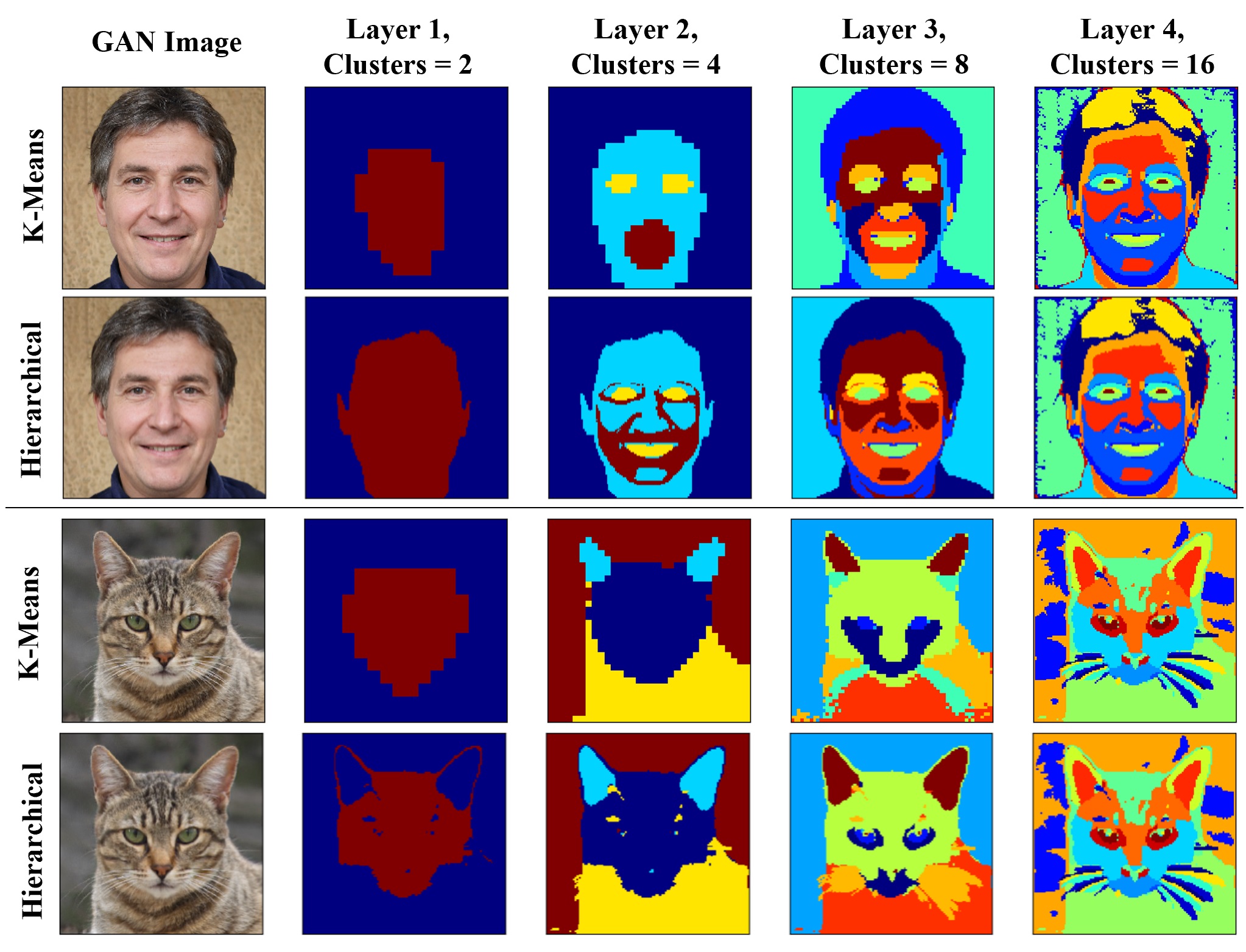
Figure 2: Segmentation using Hidden Features from a StyleGAN: The figure shows the results for unsupervised segmentation of GAN-generated images for FF-HQ and AF-HQ datasets respectively, using the hidden features extracted from a pre-trained StyleGAN generator. The first and the third rows show the segmentation results for the K-Means clusterer used in Pakhomov . [37] for individual GAN layers while the second and the fourth rows depict the clustering results obtained with hidden features from all StyleGAN layers using hierarchical merging. Both methods depict the utility of the GAN hidden features for unsupervised segmentation.

Generative adversarial networks (GANs) are trained for image synthesis by learning to map a randomly-sampled lower-dimensional latent vector to a full-scale image using deep neural networks. For a sequential GAN, such as Goodfellow . [20], this is done by passing the latent vector through a series of convolutional layers that transform it into an output image. For a style-based GAN [26], it is a constant vector that is passed through these layers while latent vectors are injected into every layer via adaptive instance normalization [22]. For both cases, the latent vector-to-image mapping is carried out by processing a lower-dimensional vector with a sequence of convolutional layers that gradually expand it into a full-scale image.

What’s interesting is that in the process of being trained to map a latent vector to an image, the hidden layers of a GAN learn the intermediate feature representations at different scales for the generated image. Several works have therefore utilized these multi-scale features to predict semantic labels for the different parts of a GAN generated image. For example, Pakhomov . [37] uses these features to perform unsupervised semantic segmentation of the synthetic images generated using a StyleGAN. This is done by picking a single layer from the GAN generator and applying K-Means clustering to the hidden features of the selected layer. The results of such clustering for different GAN layers are shown in the first and third rows of Fig. 2. The figure also illustrates the unsupervised segmentation results obtained by clustering all the GAN hidden features hierarchically with bottom-up merging. In either case, we can see that a simple clustering of the hidden features can partition the image into semantically meaningful regions.

The utility of GAN hidden features for few-shot segmentation has been explored in Y. Zhang . [51] and Tritrong . [42] by feeding the hidden features directly to a segmenter network for few-shot learning. Using the hidden features directly, however, causes the model to be biased towards the training data when limited to a single sample. This is because the effective feature space spanned by the entire hidden feature set is too large to be learned from one sample (For example, grouping all the hidden features together for the StyleGAN model used in the example in Fig. 2 results in a $5376\times 256\times 256$ feature vector for segmentation).

In our implementation, we propose an alternative self-supervised approach to one-shot segmentation. Our approach adds a contrastive clustering model to the segmentation process that first maps the hidden features onto a smaller encoded space and is later fine-tuned with a single training sample for segmentation. To that end, in the next section, we will describe the SwAV-based contrastive clustering model that we have utilized for self-supervised learning in our framework.

3.2 Self-Supervision for Image Segmentation

Before delving into a description of our proposed method, we provide, in this subsection, an overview of how contrastive learning works for one-shot image classification and the challenges faced when extending the same approach to image segmentation. The design motivations behind our implementation are to address these challenges for the segmentation of GAN-generated images.

3.2.1 Contrastive Learning for Image Segmentation

The principle of contrastive learning, as enunciated in Le-Khac . [30], makes it naturally effective for few-shot learning. By definition, it involves applying transformations to image samples within a dataset and setting up a loss function to minimize the similarity distance between the transformed versions of the one dataset image while maximizing the same between those transformed from all other classes. The learnt representations obtained by minimizing this contrastive loss serve as intermediate feature vectors for the unlabeled data that can be later used for downstream supervised learning with fewer training data requirements. This logic for contrastive learning is explained in Fig. 3.

For the framework in the figure, contrastive learning begins by first augmenting the input image using a fixed set of transformations, $\mathcal{T}$ and designating the transformed images thus obtained, $\{\textbf{x}_{t}|\>\>t\sim\mathcal{T}\}$, as the set of similar or ‘positive’ instances for the sample (also referred to as views). Likewise, image views obtained from other samples are considered as dissimilar or ‘negative’ instances for the given sample. With these positive and negative instances, contrastive loss can be computed for the projected representations $\{\textbf{z}_{t}|\>\>t\sim\mathcal{T}\}$ using a suitable similarity measure $sim(\cdot,\cdot)$ as follows:

$$\mathcal{L}\left(\textbf{x}_{i},\textbf{x}_{j}\right) =\>l_{+}\left(\textbf{z}_{si},\textbf{z}_{ti}\right)\>\>+\>\>l_{-}\left(\textbf{z}_{si},\textbf{z}_{tj}\right)$$ (1)

$$=\>\textbf{Y}\cdot sim\left(\textbf{z}_{si},\textbf{z}_{ti}\right)+$$

$$\>\>\>\>\>\>\>(1-\textbf{Y})\cdot\max\left\{0,\tau-sim\left(\textbf{z}_{si},\textbf{z}_{tj}\right)\right\}$$

Here, the contrastive loss is calculated by transforming samples $\textbf{x}_{i}$ and $\textbf{x}_{j}$ using the image transforms $s,\>t\sim T$ respectively. For the formulated loss, Y denotes the flag specifying positive sample pairs, $\tau$ determines the loss sensitivity to negative samples and the rest of the notations are adopted from Fig. 3.

While the central logic of a contrastive learner makes it ideal for one-shot learning, its effectiveness depends largely on one’s definition of what constitutes a negative instance for a given data sample. For domains and datasets where this is not possible, representation learning with contrastive methods becomes a challenge. Furthermore, the pairwise comparison between different images sampled from the unlabeled dataset, as expressed in Equation 1, is not scalable.

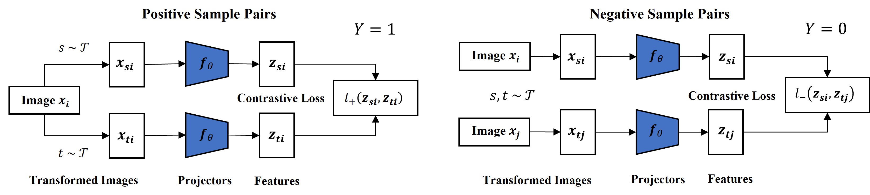
Figure 3: Contrastive Learning for Image Classification: The figure shows the signal flow visualization for computing a contrastive loss for image classification. The computation begins by transforming input samples using transforms $s,t$ selected from a fixed set of transformations $\mathcal{T}$ and then comparing the projected latent representations $\textbf{z}_{s},\textbf{z}_{t}$ between similar and dissimilar samples. The computed loss minimizes the distance $l_{+}(\cdot,\cdot)$ between positive image pairs transformed from the same sample while maximizing the distance $l_{-}(\cdot,\cdot)$ between negative ones.

These issues with contrastive learning become even more pronounced when considered in the context of image segmentation where the loss is computed at the pixel-level. For image segmentation, you are also faced with the challenge of selecting the transforms required by the logic of contrastive learning since they must be applied to the individual pixels separately. In Fig. 3, the set of transformations, $\mathcal{T}$, comprises of geometric and color-based transforms such as rotation, cropping and color jittering which operate on an entire image instance at a time. For segmentation, however, contrastive learning would need to take place at the pixel-level, hence, the transformed views must also be defined locally for every image pixel Chaitanya . [9]. Whole-image based transformations such as rotation and scaling fail to be effective for this task. In Section 4.1, we take a closer look at image augmentation strategies that allow us to formulate pixel-level contrastive losses for GAN images.

In the next subsection, we explain the SwAV algorithm that addresses some of these issues for contrastive learners.

3.2.2 Contrastive Learning with Swapped Assignment Between Views (SwAV)

Figure 4: Contrastive Learning with SwAV: The figure depicts the steps for contrastive loss computation using Swapped Assignment between Views (SwAV) [8]. Computation begins by picking a batch of $B$ images X, transforming them via a pair of fixed transformations $s,t\sim\mathcal{T}$ and projecting them into the space C spanned by the prototype vectors, one for each of the $K$ putative clusters in the training data. This yields the codes $\textbf{Q}=(\textbf{q}_{i}|\>i=1\dots B)$ for each of the batch images. Subsequently, through a solution to an on-line minimization of a transport criterion, the otherwise continuous values for the codes are mapped to cluster-assignment probability scores $\textbf{Q}^{*}=({\textbf{q}^{*}}_{i}|\>i=1\dots B)$. The crossed red lines in the figure are to be construed as an evaluation of the cluster assignment probabilities in one arm of contrastive learning vis-a-vis the projections generated in the other arm.

Fortunately, the issues with pure contrastive learning as described in the previous subsection can be addressed by inserting a clustering step before the invocation of similarity metrics. Stated very simply, this amounts to representation learning vis-a-vis the cluster labels assigned to different samples. An implementation of this is in the SwAV (Swapped Assignment between Views) mechanism [8] that uses such cluster assignments to fashion a self-supervised contrastive loss for visual feature learning. This subsection explains the SwAV mechanism and also how this clustering approach can be scaled to large uncurated datasets efficiently.

As should be evident from the caption of Fig. 4, the main conceptual difference between the contrastive learning depicted in Fig. 3 and the SwAV based approach is the projection of the batch images in each arm of the dataflow into the prototype space being learned, estimation of the cluster assignments for each batch image and the evaluation of these assignments in each arm vis-a-vis the projections in the other arm. This contrastive evaluation is carried out through the SwAV loss that is a sum of the cross-entropy losses in each arm of Fig. 4 as defined by:

$$L(\textbf{Z}_{s},\textbf{Z}_{t})=\ell(\textbf{Z}_{s},\textbf{Q}^{*}_{t})+\ell(\textbf{Z}_{t},\textbf{Q}^{*}_{s})\vspace{-2mm}$$ (2)

with

$$\ell(\textbf{z}_{si},\textbf{q}_{ti}^{*}) =-\sum_{k=1}^{K}q_{k,ti}^{*}\log p_{k,si}$$ (3)

$$=-\sum_{k=1}^{K}q_{k,ti}^{*}\log\frac{\exp(\textbf{c}_{k}^{T}\textbf{z}_{si}/\tau)}{\overset{K}{\underset{k^{\prime}=1}{\sum}}\exp(\textbf{c}_{k^{\prime}}^{T}\textbf{z}_{si}/\tau)}$$

where $\tau$ is the temperature of the loss, $i$ denotes the $i^{th}$ sample from the image batch of size $B$ and the rest of the notations are as displayed in Fig. 4. Here, the term $\textbf{c}_{k}$ represents the prototype vectors which are used for calculating the cluster assignments and which are defined ahead.

The formulation of the cross-entropy loss shown above is based on the expectation that its minimization would train the projection network $\textbf{f}_{\theta}$ to map each batch image as closely as possible to the prototype vector corresponding to its assigned cluster.

This raises the question of how each image in a batch can be given a cluster assignment efficiently and accurately for loss propagation during every training iteration.

The solution to this problem comes from Asano . [3] where the cluster assignment problem is cast and solved as an instance of an optimal transport problem. In this approach, the image features Z are first projected onto a space spanned by learnable prototype vectors $\textbf{C}=\{\textbf{c}_{1},\textbf{c}_{2},\ldots,\textbf{c}_{K}\}$ and our goal is then to determine an optimal cluster assignment $\textbf{q}^{*}_{i}$ for each of the projections $\textbf{C}^{T}\textbf{z}_{i}$. Recall that $i$ is the batch image index. Caron . [8] formulates the search for the optimal $\textbf{Q}^{*}$ as the following minimization problem for optimal transport:

$$\underset{\textbf{Q}\in\mathcal{Q}}{\arg\min}\left<\textbf{Q},-\textbf{C}^{T}\textbf{Z}\right>+\upvarepsilon\cdot H(\textbf{Q})$$ (4)

where the additional entropy term $H(\textbf{Q})$ serves as a regularizer. It was shown in Cuturi [16] that this regularizer allows for the following analytical solution to the minimization problem stated above:

$$\textbf{Q}^{*}=Diag(\textbf{u})\cdot\exp\left(\frac{\textbf{C}^{T}\textbf{Z}}{\upvarepsilon}\right)\cdot Diag(\textbf{v})$$ (5)

where $\textbf{Q}^{*}$ is the optimal solution for translating the codes Q into cluster assignment probabilities for the individual images in a batch and where u and v are renormalization vectors computed using the iterative Sinkhorn-Knopp algorithm. A more detailed formulation of the optimization problem in Equation 4 and its solution as shown in Equation 5 are presented in the appendix. The advantage of the analytical solution in Equation 5 is that the clustering can be performed in as few as three iterations of the Sinkhorn-Knopp algorithm which allows for a fast computation of the SwAV loss for self-supervised learning.

The scalability of the SwAV method for larger datasets makes it especially useful for image segmentation which requires calculating the contrastive losses at each pixel. Recent works [53] have already demonstrated the utility of SwAV clustering for unsupervised image segmentation. In the next section, we explain our GAN-based framework that uses the SwAV model for carrying out the hidden feature clustering required in our one-shot segmentation model.

4 Our GAN-Adaptation of SwAV-Based Clustering

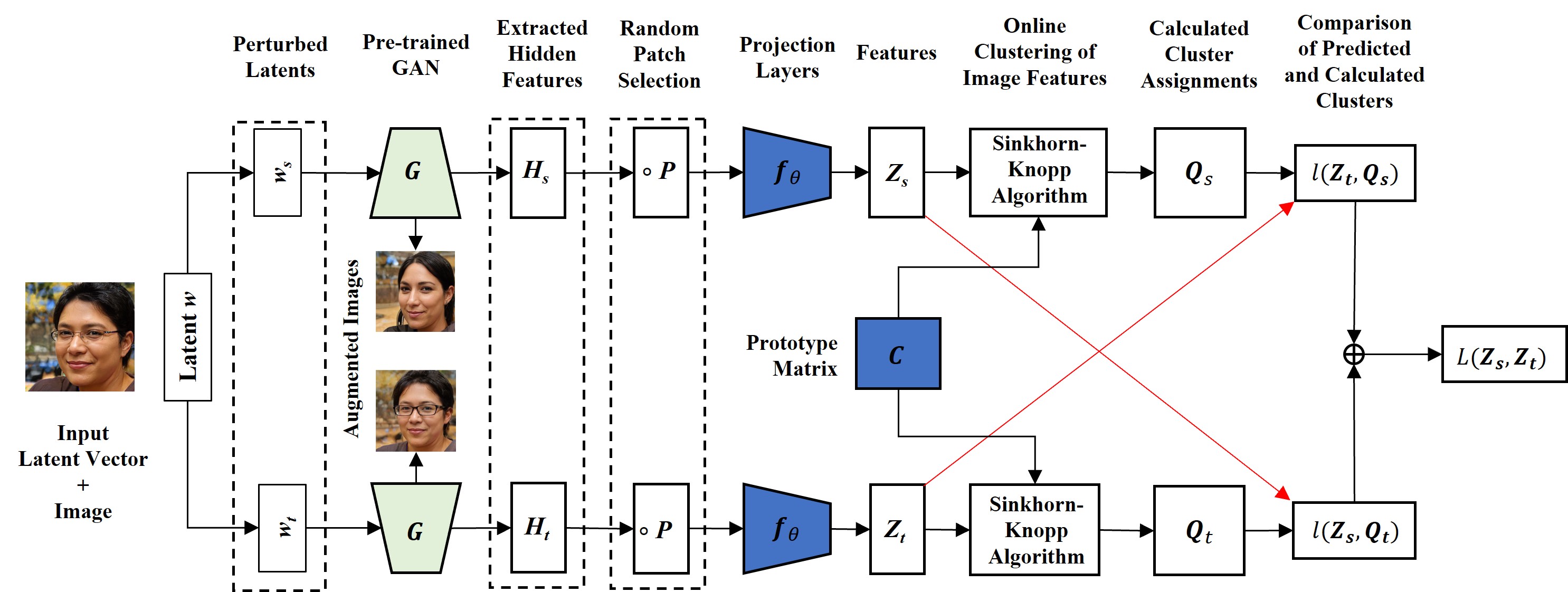
Figure 5: Our Adaptation of the SwAV-based Contrastive Learning for Pixel-Level Clustering in a GAN: Image augmentation for the SwAV model is performed using latent vector perturbations as explained in Section 4.1. The SwAV loss is calculated using the hidden features extracted from the GAN during image synthesis and is formulated in Section 4.2.

Fig. 5 illustrates how we have adapted the self-supervised SwAV approach to our needs for clustering the pixels (each pixel being a vector of hidden features) in a GAN-generated image. To summarize what is depicted in the figure, the training data generation begins with the latent vectors fed into the GAN generator. Subsequently, white-noise perturbed versions of the input latent vector, $\textbf{w}_{i}$ are used to create augmented versions of the original image. Finally, the hidden features are extracted for the resulting transformed images from the pretrained StyleGAN and subsequently used for SwAV loss calculation.

Note that there are two main differences between the general SwAV model shown in Fig. 4 and the one in Fig. 5: The first difference is with regard to how image augmentations are carried out for computing the contrastive loss. And the second difference is in the formulation of the SwAV loss itself. Both of these steps are explained in what follows.

4.1 Image Augmentation via Sampling in $\textbf{W}^{+}$ Space

In our proposed framework in Fig. 5, the augmented data for contrastive loss calculations is not generated via fixed image transformations like those used in the original SwAV model in Section 3.2.2. Instead, we have taken advantage of the latent space properties of the StyleGAN2 architecture [27] to introduce a new data augmentation method for GAN-generated images. The core idea behind our proposed method is to augment a GAN-generated image by sampling a new latent vector in the vicinity of the original vector that produces the image. Because of the perceptual smoothing properties of StyleGANs [27], the image produced by the new latent vector shares most of its features with the original image and can be used as an augmented variant of the same. How this is done is described as follows:

Since different latent vectors are fed in parallel into the different blocks of a StyleGAN, the images produced by the GAN can be sampled in the extended $W^{+}$ latent space spanned by those vectors [39]. This extended latent space uses a set of latent vectors, $\{\textbf{w}_{i}|\>i=1,\ldots,L\}$ wherein each vector, $\textbf{w}_{i}$ is associated independently with the i^th style block of an $L$-layer generator.

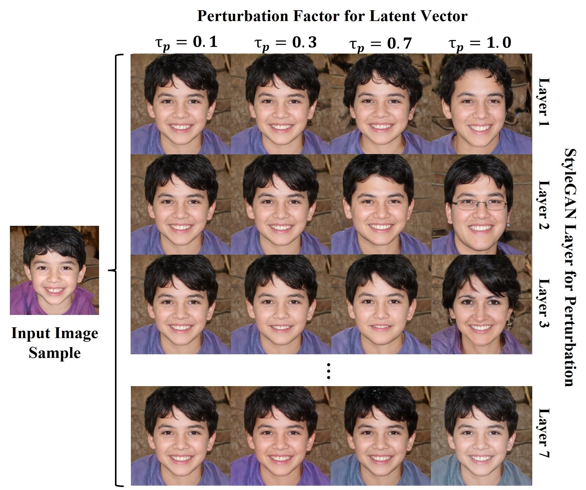
Figure 6: Image Augmentation via Sampling in $\textbf{W}^{+}$ latent space: The figure shows the augmented image samples produced by perturbing the extended latent vectors at different StyleGAN layers. The perturbed layer determines the scale at which the image properties are affected while the perturbation factor $\uptau_{p}$ determines the sampling diversity.

For each generated image, therefore, our framework creates new image samples by perturbing the extended latent vectors for one of the style blocks to produce similar synthetic images as the original image. Examples of these augmentations are shown in Fig. 6 where a GAN image is augmented using the extended latent vectors $\{\textbf{w}_{i}|\>i=1,\ldots,L\}$ associated with it.

Now, for every $i^{th}$ style block, a different image sample can be produced by simply perturbing the latent vector $\textbf{w}_{i}$ with a zero-mean noise vector:

$$\textbf{w}_{i}^{{}^{\prime}}=\textbf{w}_{i}+\textbf{n}_{d}=\textbf{w}_{i}+\mathcal{N}(0,\sigma_{d}^{2}\cdot\textbf{I})$$ (6)

where $\sigma_{d}$ determines the extent of perturbation. However, the StyleGAN latent space $\mathcal{W}$ is not uniformly distributed. The distribution is a result of mapping the uniform latent space $\mathcal{Z}$ to a disentangled space that is more representative of the training data distribution [26]. Hence, the new latent vector $\textbf{w}_{i}^{{}^{\prime}}$ obtained from the above equation will not always point towards a valid image in the latent space. This can lead to noisy or distorted images generated from the augmented latent obtained in this manner.

For our model, we instead use a latent interpolation-based approach for augmenting the GAN images. The augmented latent vector $\textbf{w}_{i}^{{}^{\prime}}$ is formed by mixing w with the latent vector of a randomly sampled image as follows:

$$\textbf{w}_{i}^{{}^{\prime}}=\uptau_{p}\cdot\textbf{w}_{i}+(1-\uptau_{p})\cdot\textbf{w}_{i}^{(p)}$$ (7)

where $\textbf{w}_{i}^{(p)}$ is the latent vector for the $i^{th}$ style block for a new randomly sampled image. This allows us to control the diversity in the augmented image samples by adjusting the perturbation factor $\uptau_{p}$ in Equation 7. The advantage of this method can be seen in Fig. 7 where we compare the augmented images generated by the two different approaches. We can see that the stability provided by our interpolation-based approach rids the augmented images of the artifacts seen in the images obtained from Equation 6.

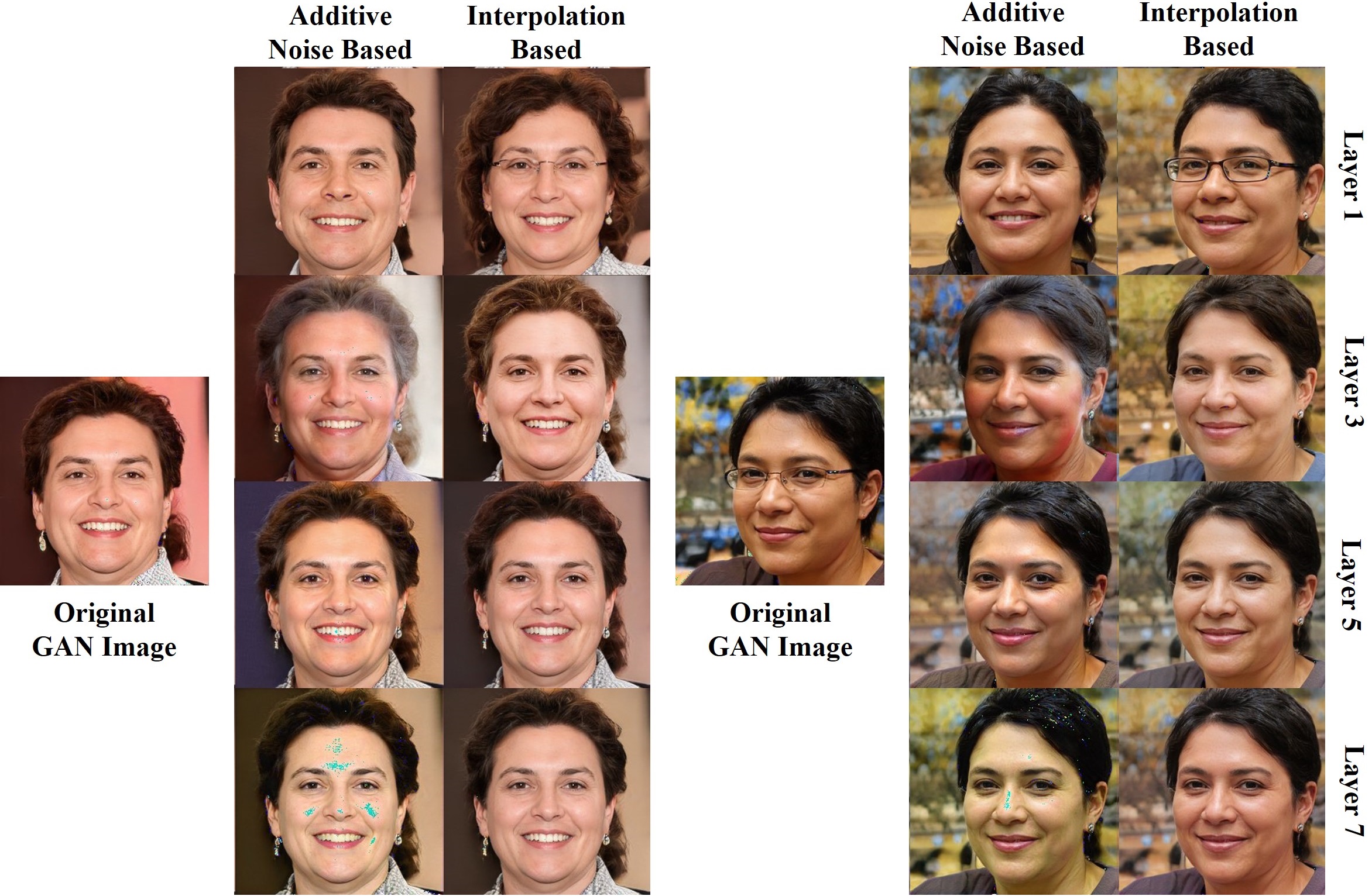
Figure 7: Comparison of Methods for Latent Vector Perturbation: The figure compares the augmented image samples produced via latent vector perturbation using the additive noise-based method (left) and the interpolation-based method (right). The outputs are compared for latent vectors perturbed for different StyleGAN layers and with a perturbation factor, $\uptau_{p}=1.0$. We can see that our interpolation-based approach is able to generate noise-free images compared to the other method.

As made evident by Fig. 6, perturbing the latent vectors for different style layers changes the image features at different scales depending on the scale of the output activations produced by that style layer. Hence, perturbing the latent vectors at the deeper layers of the GAN results in varying local features such as color and texture whereas perturbing the initial layers controls the more semantic properties of the image (such as age and gender in the examples of Fig. 6). As explained in the next section, this plays an important role in the formulation of our SwAV loss for image segmentation.

4.2 SwAV Loss formulation

Once the augmented input images are generated through latent vector perturbations, our next step for the SwAV model in Fig. 5 is to extract pixel-wise hidden features from the layers of the GAN generator for self-supervised clustering. This extracted set of features is what is used to compute the projections $\textbf{Z}_{s},\textbf{Z}_{t}$ for obtaining the cluster assignments and thereafter the swapped prediction loss. Now, since the layers of the GAN generator have different spatial sizes, the output of each layer must first be scaled up to match the size of the final output image. Therefore, the extracted hidden features $\textbf{H}_{1},\textbf{H}_{2},\ldots,\textbf{H}_{L}$ from the $L$-layer StyleGAN generator are first upsampled to the size of the output image and subsequently concatenated together to form feature vectors that take the following form:

$$\textbf{H}=\mathds{U}_{H\times W}(\textbf{H}_{1})\otimes_{c}\ldots\otimes\mathds{U}_{H\times W}(\textbf{H}_{L})$$ (8)

where the notation is borrowed from Tritrong . [42]. $\mathds{U}_{H\times W}(\cdot)$ denotes the upsampling operation to the image dimension $H\times W$, $\otimes_{c}$ denotes the concatenating operator and the feature vector H is computed for StyleGAN layers from $1$ through $L$. With these computed feature vectors, we now turn to the calculation of our SwAV loss. The product $H\times W$ of all hidden features can result in excessively large batch sizes for clustering, hence, the SwAV loss in our model is computed using randomly selected pixels or pixel patches from the image. The image features for our SwAV loss are thus calculated as:

$$\textbf{Z}_{s} =\textbf{f}_{\theta}\left(\hat{\textbf{H}}(\textbf{w}_{s})\circ\textbf{P}_{i,j}\right);$$ (9)

$$\textbf{Z}_{t} =\textbf{f}_{\theta}\left(\hat{\textbf{H}}(\textbf{w}_{t})\circ\textbf{P}_{i,j}\right)$$

where the image indices $i,j$ are randomly picked for the image patch P in each training iteration. The operator $\hat{\textbf{H}}(\cdot)$ denotes the features extractor that yields the hidden feature vector H for a latent input. With these features, we express the overall swapped prediction loss for our model as a sum of a ‘global’ component and a ‘local’ component:

$$L_{HFC}=L_{global}(\textbf{Z}_{s},\textbf{Z}_{t})+L_{local}(\textbf{Z}_{s},\textbf{Z}_{t})$$ (10)

with $s,\>t$ being the respective perturbed layers for the two image transformations. Here, the SwAV loss for the global loss term is the same as Equation 3. On the other hand, the local SwAV loss is calculated from Equation 3 by masking the hidden features of all layers upto the perturbed layer:

$$\hat{\textbf{H}}_{local}(\textbf{w}_{s})=\textbf{M}_{1,{s-1}}\circ\hat{\textbf{H}}(\textbf{w}_{s})$$ (11)

Here, $\textbf{M}_{1,{s-1}}$ is defined for a perturbed layer $s$ and masks out all the channels of the generated feature vector H that correspond to the layers $1$ to $s-1$. The intuition behind the local SwAV loss is as follows:

In Section 3.2.1, we talked about the need for contrastive losses for image segmentation to capture the local image properties for per-pixel classification. Our formulation of the local SwAV loss described above addresses this need by using the hidden layer properties of StyleGAN models. We have seen that the style features extracted from the different GAN layers pertain to the image properties at different scales and that perturbing the extended latent vector for a given layer triggers changes in the image features at that scale. Since the style layers of a GAN generator are connected sequentially, perturbing the latent vector for the $s^{th}$ layer for image transformation only affects the hidden features for layers starting from the $s^{th}$ layer. Hence, the local loss term in Equation 10 provides a ‘localized’ calculation of the SwAV losses by neglecting the unperturbed hidden features of the transformed image.

The image augmentation strategy described in Section 4.1 and the loss formulated in Section 4.2 provide us with a SwAV-based model for self-supervised clustering of the GAN hidden features. Once trained, this model yields pixel-wise cluster predictions for synthetic images as they are being produced by the GAN. In the next section, we conclude our framework description by explaining how on-the-fly, automatic segmentation is carried out with this setup using one-shot segmentation.

5 Automatic Segmentation with One-Shot Learning

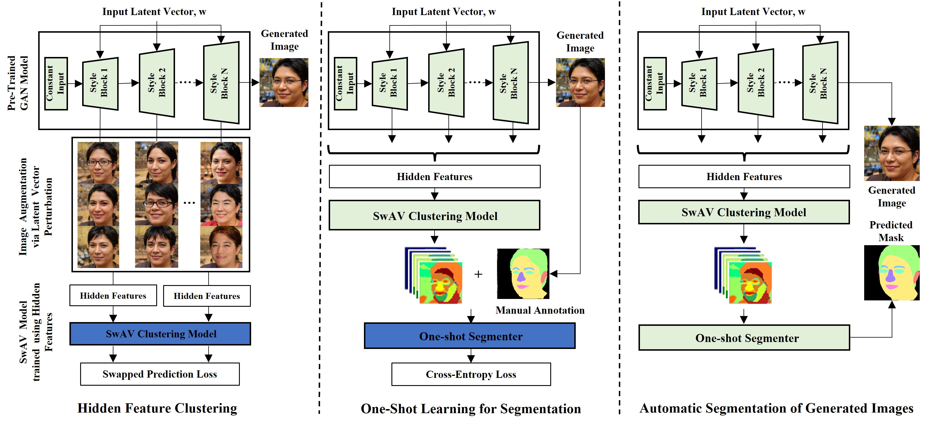
Figure 8: Training and Inference Operations for our Implementation: The figure shows the different stages of operation of our implemented framework: (i) Hidden Feature Clustering: Here, a SwAV-based model is used for the pixel-wise clustering of hidden features extracted for a GAN-generated image. This model is described at length in Section 4. (ii) One-Shot Learning for Segmentation: Once the clustering model is trained, the feature outputs from the model are used by a segmenter network for one-shot learning of segmentation masks. (iii) Automatic Segmentation: After the clustering and segmenter models are trained, synthetic images can be automatically segmented as they are being generated by the GAN.

So far we have talked about how self-supervised clustering is performed for the GAN hidden features in our implementation. In this section, we describe how we perform the on-the-fly segmentation of GAN-generated images via one-shot learning enabled by this model.

As mentioned in the Introduction, our ultimate aim is to enable automatic segmentation of synthetic images as they are being generated by a GAN. To do so, we make use of a single manually labelled sample that serves as a guiding sample to learn to automatically segment similar image regions in newly synthesized GAN images. We set up our framework for this task by training it in two stages. During the first stage, the network learns the pixel-wise representation space for the unlabeled images generated by a GAN. This is done using our SwAV model from Section 4. Subsequently, during the second stage, a second network is trained to apply the learned representation space to a specific segmentation task which is defined by the manually labelled sample.

Once both clustering and fine-tuning operations are complete, the framework is ready for on-the-fly segmentation of GAN-generated images. As a latent vector is fed to the GAN for image generation, hidden features are extracted and fed to the trained clustering model to produce pixel-wise feature vectors for the image. The segmenter then uses these feature vectors to predict the segmentation masks for the generated image. Fig. 8 is a depiction of the training and inference operations described above.

In the rest of the paper, we discuss the different experiments that have been conducted on the proposed framework to assess its performance for one-shot segmentation.

6 Implementation and Testing

6.1 Datasets

Table 1: Dataset Specifications for StyleGAN Pre-Training and One-Shot Segmentation: The table lists the details for labeled and unlabeled image datasets that we have used in our experiments to evaluate our framework for different test classes. The first section of the table lists the unlabeled datasets on which the StyleGAN models have been pre-trained for the different test classes. The second section of the table lists the details for annotated datasets whose samples are used for training and evaluating the one-shot learning framework.

Test Class	Unlabeled Datasets				Annotated Datasets
	(StyleGAN Pre-Training)				(One-Shot Testing)
	Dataset	Samples	Resolution	Layers	Dataset	Samples	Parts
Face	FF-HQ1	$7\times 10^{5}$	$1024\times 1024$	8	CelebAM-HQ2	$30,000$	19
Cat	LSUN3, AFHQ4	$1,672,266$	$256\times 256$	6	LSUN3	$333$	17
Car	LSUN3	$5,520,756$	$512\times 384$	7	PASCAL-P5	$139$	13
Horse	LSUN3	$2,000,340$	$512\times 512$	6	PASCAL-P5	$60$	21

¹ Flickr-Faces-HQ Dataset [26],  ² CelebA-MaskHQ Dataset [29],
 ³ LSUN Dataset [47]  ⁴ Animal-Faces HQ Dataset [15]
 ⁵ PASCAL-Part Dataset [13]

Table 1 lists the different datasets that we have used to train and evaluate our framework. As shown in the table, we have divided our experiments into the following four test classes based on the objects of interest for segmentation: (i) Face, (ii) Cat, (iii) Horse and (iv) Car. For each class, we have used two different datasets for evaluation: (i) The first dataset is a large-scale unlabeled dataset on which the GAN model is pre-trained for image synthesis. And (ii) the second dataset is a small-size labeled dataset wherein the samples have been annotated with segmentation labels and are used to train and evaluate the one-shot learning model.

The first section of Table 1 lists the different unlabeled datasets used for pre-training the StyleGAN models for image synthesis. The table also mentions the size of the StyleGAN model being pre-trained. Here, two main datasets are made use of for pre-training the models: For the Face class, we use a StyleGAN2-ADA model that is pre-trained on the Flickr-Faces-HQ dataset [26] to generate human faces. For the other three classes, models trained on the LSUN dataset [47] are used which contains more than $1\times 10^{6}$ samples for each class. For the Cat class, the Animals Faces-HQ [15] dataset is also additionally used.

To test the segmentation performance of our framework, we used the annotated datasets that contain segmentation masks for different parts of the test classes listed in Table 1. For example, the annotated dataset for the Face class is the CelebA-MaskHQ dataset [29] that contains 30,000 images of celebrity faces labeled with segmentation masks for 19 different parts of the face (eyes, ears, mouth etc.). Similarly, for the other classes, the PASCAL-Part dataset [13] is used which consists of labeled image samples for the Car, Cat and Horse classes. The details for all these datasets are listed in Table 1. Additionally, 30 new test samples were manually annotated for each test class for the ablation studies and demonstration. These annotations as well as segmentation results on additional datasets are available in the code repository associated with this submission.

6.2 Framework Specifications

This subsection describes the setup and specifications of the different blocks of our implemented framework:

6.2.1 Pre-Trained StyleGAN Models

Our framework uses the StyleGAN2-ADA architecture [25] for model pre-training for the purpose of image generation for all test classes. The pre-trained weights for these models have been obtained for each of the four test classes from NVIDIA’s official GitHub repository on StyleGANs . Each model processes latent vectors of dimensions $1\times 512$ to produce the synthetic images. The image resolution for the each model is also listed in Table 1.

6.2.2 Image Augmentation

The image augmentation strategy that is described in Section 4.1 is defined by two parameters: the StyleGAN layer being perturbed and the perturbation factor, $\uptau_{p}$ from Equation 7. For our implementation, we have used a perturbation factor of $\uptau_{p}=0.9$ to maximize sampling diversity. The StyleGAN layer for perturbation is randomly chosen for each training iteration. In the ablation studies in Section 9, we have also analyzed the effect of varying the perturbation parameters on the overall framework performance.

6.2.3 Hidden Feature Clustering

The input to the SwAV clustering model from Fig. 5 is a $1\times 512$ latent vector w which generates the synthetic image from the StyleGAN model as well as the pixel-wise hidden feature representations. These representations are of dimensions $(C_{hidden}\times H\times W)$ where $C_{hidden}$ is the effective length of the hidden features calculated from Equation 8 and $H\times W$ denote the image dimensions. From the feature representations extracted for a sample, our framework uses $5-10$ randomly cropped image patches of size $64\times 64$ to calculate the SwAV loss during training.

The projection network $\textbf{f}_{\theta}$ for the clustering model consists of a single dense layer followed by a leaky ReLU activation that encodes the hidden representations into more compact feature vectors $\textbf{z}\in\mathds{R}^{D}$. The feature dimension $D$ is chosen based on the number of prototype vectors $K$ used for cluster assignments. In our implementation, a total of $K=4000$ prototype vectors with a feature dimension of $D=512$ are used for the SwAV model.

Our SwAV model was trained for 100 epochs where each epoch comprised of a set of 1-50 randomly sampled images from StyleGANs. The model was trained using an SGD optimizer [46] with layerwise scaling [46], a learning rate of $0.01$ and a momentum of $0.9$ while the SwAV loss in Equation 3 was computed with a temperature of $\tau=0.01$. For computing cluster assignments, the Sinkhorn-Knopp algorithm was implemented using $10$ normalizing iterations and with $eps$ set to the value of $0.005$. The hyperparameters for Sinkhorn iterations and patch selection were adjusted for each test class for optimal performance and the exact values can be obtained from our code repository.

6.2.4 One-Shot Segmentation

We have tested the performance of our framework using a range of different segmenter models for on-the-fly, one-shot segmentation. This was done to ensure that the observed performance of the framework is not influenced by our choice of the downstream segmenter. The first two segmenters used for our tests comprise of a a single-layer and a three-layer dense neural network each terminating with a softmax layer. The rest are fully convolutional networks implemented with different number of hidden layers (3, 5, 7 and 9 layers). For these networks, each convolutional layer is constructed with a unit stride, a $3\times 3$ kernel size and followed by a leaky ReLU activation (except for the last layer which terminates with a softmax activation).

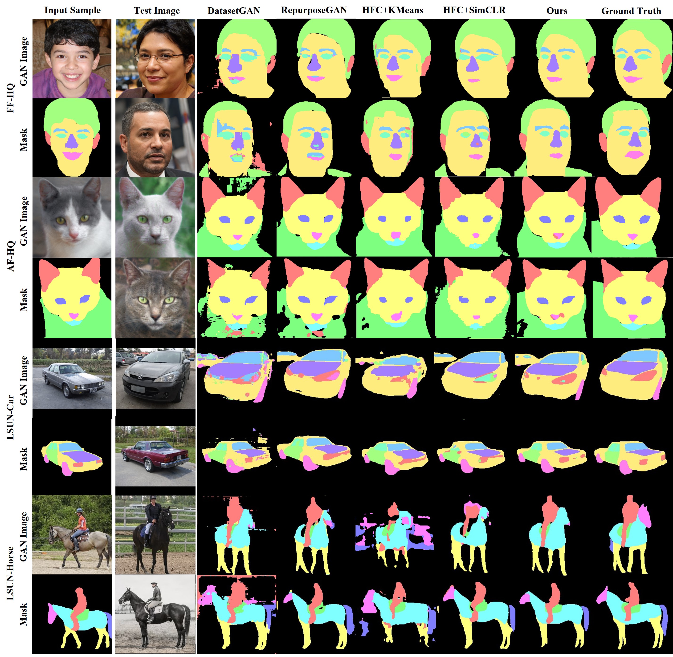
Figure 9: One-shot Segmentation using the Proposed Framework: The figure shows the one-shot segmentation performance of our proposed method against other baseline methods for the four test classes (Face, Cat, Car, Horse). The first column depicts the input image sample and its user-specified annotations. The second column shows the test images generated by the GAN and the rest of the columns denote the mask predictions from different segmenters. The last column denotes the ground truth segmentation mask for the test images.

For both cases, the segmenter is trained on feature vectors H and one-shot annotation masks for $200$ epochs using a cross entropy loss and an Adam optimizer with the hyperparameters set at: $\{learning\_rate=0.01,\beta=(0.9,0.99)\}$. Unless otherwise specified, the default segmenter used in our framework is a 3-layer convolutional neural network.

7 Experiments and Results

7.1 Tests for one-shot segmentation

Table 2: Performance Comparison for One-shot Segmentation with other Baseline Methods: The table compares the (wIoU, FG-IoU) performance values for our method against semi-supervised and self-supervised baselines. For the self-supervised methods, the values are shown for two different one-shot segmenters: a single layer MLP and the 3-layer fully convolutional network (FCN) described in Section 6.

Baseline Category	Method	OSS	Face	Cat	Car	Horse
Semi- Supervised	DatasetGAN	-	$(49.48,\>\>91.68)$	$(18.75,\>\>73.15)$	$(16.84,\>\>88.97)$	$(9.79,\>\>87.12)$
	LAGM	-	$(52.81,\>\>92.90)$	$(21.48,\>\>92.12)$	$(18.88,\>\>95.40)$	$(\textbf{10.16},\>\>88.10)$
	RepurposeGAN	MLP	$(51.43,\>\>91.88)$	$(21.44,\>\>87.67)$	$(17.68,\>\>95.04)$	$(8.99,\>\>82.42)$
		FCN	$(51.46,\>\>91.92)$	$(20.55,\>\>89.91)$	$(\textbf{18.99},\>\>94.74)$	$(9.89,\>\>88.53)$
Self- Supervised	HFC + KMeans1	-	$(48.92,\>\>92.83)$	$(13.81,\>\>64.05)$	$(12.11,\>\>90.69)$	$(6.74,\>\>85.35)$
	HFC + SimCLR2	MLP	$(50.36,\>\>92.09)$	$(19.96,\>\>91.60)$	$(16.24,\>\>94.36)$	$(8.17,\>\>86.51)$
		FCN	$(50.32,\>\>92.28)$	$(16.36,\>\>82.99)$	$(16.01,\>\>95.41)$	$(9.89,\>\>\textbf{88.53})$
Ours	HFC + SwAV 3	MLP	$(52.83,\>\>94.03)$	$(\textbf{21.50},\>\>93.62)$	$(18.63,\>\>95.13)$	$(9.95,\>\>87.92)$
		FCN	$(\textbf{53.61},\>\>\textbf{94.14})$	$(18.53,\>\>\textbf{94.28})$	$(18.59,\>\>\textbf{95.57})$	$(\textbf{10.16},\>\>87.63)$

¹ Hidden Feature Clustering with KMeans,  ² Hidden Feature Clustering with SimCLR,
³ Hidden Feature Clustering with SwAV,

(MLP - 1-layer dense neural network,  FCN - 3-layer fully convolutional network  OSS - Downstream One-Shot Segmenter)

The tests for one-shot segmentation have been carried out with the help of the annotated datasets listed in Table 1 for the four different test classes. To evaluate the performance, one labeled sample is picked from the annotated dataset to train the one-shot segmenter while the rest of the dataset is used for testing the segmenter predictions – performance is calculated for each test sample in terms of weighted $IoU$ for all the different object parts. The weighted $IoU$ for the predicted segmentation maps is calculated as the mean $IoU$ for all object part labels weighted by the ratios of the areas of the ground truth label mask and the whole image. The tests are repeated for 20 test samples and the mean $wIoU$ values from all these iterations are recorded as the final results. The table also lists for each test class, the mean object $IoU$ (FG-IoU) for the foreground object in the generated image of the respective test class (for example, the foreground object for the Horse class is the horse itself).

The performance results for one-shot segmentation have been listed in Table 2. DatasetGAN [51], RepurposeGAN [42] and LAGM [45] have been used as the semi-supervised baseline methods for comparing the $IoU$ performance. For self-supervised baselines, we have included the performance of a version of our framework wherein hidden feature clustering is carried out by a K-Means algorithm [7] and another version which uses the SimCLR model [11]. We see that when the training data size is restricted to a single sample, the proposed method fairs better than the baselines in almost all cases. This is also seen in the illustrated examples in Fig. 9. A detailed breakdown of the segmentation performance for each test class is also provided in the supplementary material.

Table 3: Performance Comparison for Enhancing Supervised Computer Vision Tasks: The table lists the wIoU performance values for a supervised segmenter (DeepLabV3 - LC. Chen . [10]) when it is trained using the synthetic labeled data generated from a StyleGAN and then tested on the annotated datasets from Table 1. The values for each test class are presented for different R:A (real-to-synthetic sample) ratios in the training data.

Test Class	Face			Car			Cat			Horse
R:A Ratio	1:1	1:2	1:5	1:1	1:2	1:5	1:1	1:2	1:5	1:1	1:2	1:5
No Augmentation	68.71			66.67			54.30			36.88
DatasetGAN	69.70	70.11	73.32	67.11	68.05	70.86	56.31	58.12	58.40	37.12	40.78	41.03
RepurposeGAN	70.01	73.35	78.71	68.77	69.69	71.97	57.02	60.23	65.51	38.02	41.58	44.35
HFC+KMeans	69.07	69.91	72.03	66.83	69.12	69.32	57.19	59.45	61.03	37.00	40.22	40.79
Ours	70.12	73.56	79.57	69.04	69.51	72.57	57.14	60.02	62.32	38.21	42.97	44.37

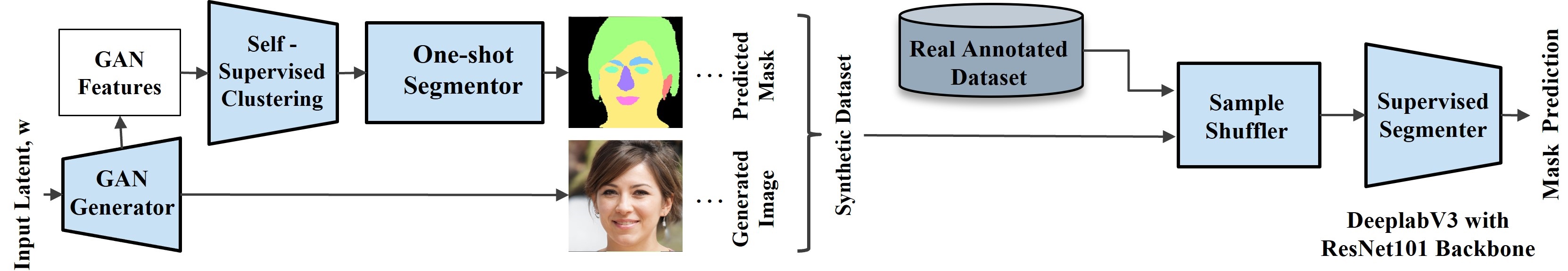
Figure 10: Dataflow for Testing the Framework Performance with Regard to Improving the Downstream Computer Vision Tasks: The figure depicts how the experiments in Section 7.2 are set up and executed. These experiments test how well the synthetic data generated by our framework can be used as a substitute for real labeled data for supervised learning. Here, the GAN-generated (label, image) pairs are first mixed with a real annotated dataset and then fed into a segmenter (DeepLabV3) for supervised training. Subsequently, any resulting improvement in mask prediction are checked for evaluating the synthetic data.

7.2 Tests with Downstream Computer Vision Tasks

In this subsection, we have examined our framework’s ability to generate labeled synthetic data that can be used to enhance the performance of supervised computer vision tasks. To do so, we first use our one-shot segmentation framework along with a pre-trained StyleGAN model to create (synthetic label, image) pairs for the different test classes from Table 1. The dataflow for this experiments is shown in Fig. 10 and is not unlike the one described in the previous section. However, here, the corpus of synthesized labelled samples is used to train a supervised segmentation network for mask prediction. The trained segmenter is then tested on a dataset of real annotated images (see Table 1). Subsequently, the performance of this segmenter is compared with another segmenter trained only on real (label, image) pairs. The comparison allows us to check how well the GAN-generated data can be used as a substitute for the real data. We have repeated this test with the other baseline methods for all four test classes. The test results are presented in Table 3 for different ratios of real and synthetic data used for training the downstream segmenter. Table 3 shows that our method performs better than the baselines especially for higher real-to-synthetic sample ratios.

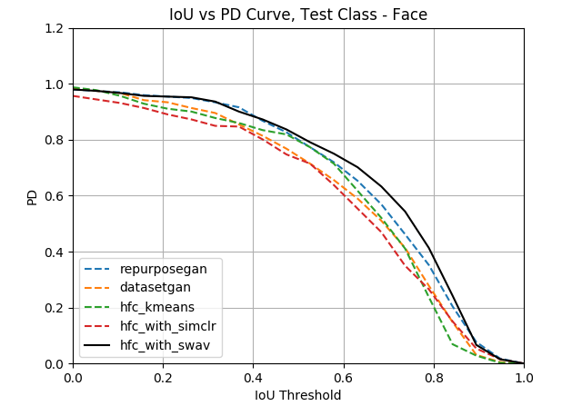
(a) Face Class

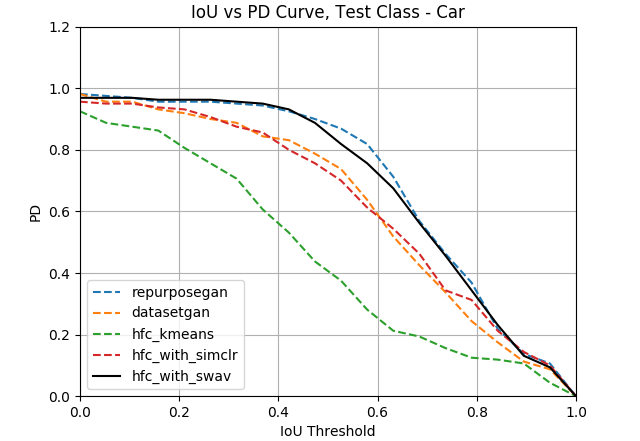
(b) Car Class

Figure 11: mIoU versus PD Curves for One-Shot Segmentation: The plot shows the IoU versus PD performance curves for the different one-shot segmenters listed in Table 2 for the Face and Car test class.

7.3 Comparison of IoU versus PD Curves

Fig. 15 expands the segmentation results for the different methods listed in Table 2 by plotting the PD (probability of detection or true positive rate) values for varying IoU thresholds. Segmentation performance can be determined from these curves by considering the cumulative number of positive predictions obtained for increasing IoU thresholds. For example, from Fig. 15, we can observe that the proposed method exhibits peak performance for Face class with $83.16\>\%$ of the predictions having an $mIoU>0.5$.

Table 4: Precision with Which Low-Frequency Object Labels are Segmented: The table compares the precision values as obtained with our framework against other baselines for segmenting out rare or low-frequency object labels. The precision values are recorded at an IoU threshold of 0.5.

Test Class	Face			Horse	Car
Label	eye_g	teeth	cloth	rider	plate
DatasetGAN	14.28	25.44	59.09	64.71	29.41
RepurposeGAN	32.33	66.67	83.33	68.75	79.57
HFC+KMeans	15.70	89.88	53.84	57.89	83.32
HFC+SimCLR	51.22	93.32	88.89	76.93	81.33
Ours	58.31	94.11	93.33	90.11	83.32

Figure 12: One-Shot Segmentation of Low Frequency Objects Labels: The figure shows the segmenter predictions using our framework and as obtained with other baseline methods for low-frequency object labels. Here, the low-frequency object labels being segmented are eye_g (glasses) for the Face test class and rider for the Horse test class. We see that our method is capable of avoiding false positives for negative samples resulting in higher precision values compared to what is achieved with the baseline methods.

7.4 Segmentation of Low Frequency Object Labels

In this section, we test an interesting property of our self- supervised framework for the segmentation of rare or low frequency object labels. This set of labels refers to the objects or attributes that may not always be present in an image sample generated by a GAN. For example, in Fig. 12, the rare object label being segmented is the eyeglass, since for a GAN generating human faces, the sampled face may or may not have eyeglasses. When poorly trained, one-shot learners tend to overfit for such annotations resulting in frequent false positives in the prediction. To test this, we have enumerated in Table 4 the precision performance of our framework and other baselines for the segmentation of five different low frequency labels (eye_g, teeth, cloth, rider, plate) from three different test classes (Face, Horse, Car).

As seen in the table and in Fig. 12, our proposed method accurately avoids these false positives when predicting segmentation masks for low frequency objects. This can be attributed to self-supervised learning models in general since the learnt self-supervised representations are free from any biases that may otherwise incur when the segmenter is trained directly on a single sample.

In the case study in Section 8, this property of our framework has been utilized for the automatic segmentation of prohibited items from baggage X-ray images for airport screening. Here, prohibited items in airport luggage can be treated as low frequency object labels as they will not be present in every bag that is scanned at an airport.

Table 5: Speed Comparison for Inference (fps)

Method	Face	Car	Cat	Horse
DatasetGAN	0.85	0.22	0.84	0.83
RepurposeGAN / MLP	0.50	0.20	0.78	0.79
RepurposeGAN / FCN	0.59	0.60	0.69	0.60
HFC + KMeans	1.19	0.94	1.17	1.20
HFC + SimCLR / MLP	1.78	2.22	1.75	1.72
HFC + SimCLR / FCN	1.24	1.25	1.29	1.27
Ours / MLP	2.27	2.32	2.27	2.29
Ours / FCN	1.23	2.39	1.29	1.21

Note: The inference speeds has been determined for the different methods using a cloud computing node with a single Nvidia Tesla V100^TM GPU, 56 processor cores and 200 GB of memory.

7.5 Comparison of Inference Times

Table 5 examines the performance of our implementation for its computational speed. It is obvious that using self-supervised learning boosts the computation time for one-shot segmentation as the model only needs to process the low-dimensional feature vectors from the clustering model. This boost can be observed in Table 5 where the fps rates for the self-supervised segmenters are about four times higher irrespective of the network architecture and dataset.

8 Case Study: The BagGAN Framework

This section is a case study involving the implementation of the BagGAN framework, where we have applied our proposed segmentation model to simulate annotated baggage X-ray scans for threat detection. Automatic detection of prohibited items from baggage X-rays scans is a challenging problem due to the limited availability of baggage screening datasets for training such automated threat detectors [35, 36]. Hence, as an alternative, we have implemented the BagGAN framework which allows for the large-scale generation of synthetic baggage images using a StyleGAN network and which also performs automatic annotation of the generated images with the proposed one-shot segmenter. The following subsections provide a summary of this baggage simulator along with a set of simulation examples for prohibited item detection.

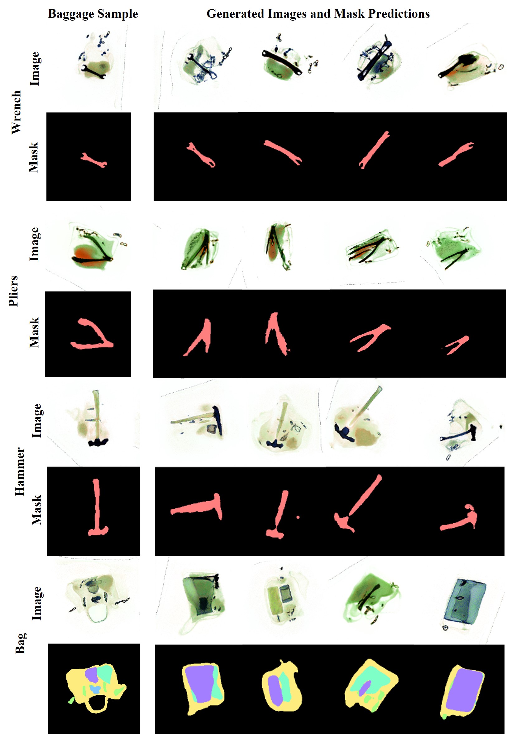
Figure 13: One-Shot Segmentation of Prohibited Items in Synthetic Baggage Images using the BagGAN Framework: The figure illustrates the automatic segmentation of prohibited items (wrench, hammer and pliers) as obtained by the one-shot segmenter in the BagGAN framework. The leftmost column shows the labeled image sample used to train the BagGAN model whereas the rest of the images show the GAN generated baggage images along with their predicted masks. The last row shows an example of a baggage image manually labeled for all of its contents.

Table 6: Performance Comparison for One-Shot Segmentation using the BagGAN framework - precision (at $IoU=0.5$) and IoU values are calculated for 5 different categories of prohibited items in the PIDRay dataset [43] for different one-shot segmenters.

Method	hammer		handcuffs		pliers		powerbank		wrench
	Prec.	IoU	Prec.	IoU	Prec.	IoU	Prec.	IoU	Prec.	IoU
DatasetGAN	44.44	51.43	27.58	43.72	27.58	48.62	37.50	52.37	44.82	51.42
RepurposeGAN	54.16	60.56	37.93	51.02	33.33	55.29	53.33	57.49	48.14	61.58
HFC+KMeans	36.11	50.82	64.28	51.13	52.50	51.71	48.27	55.06	58.82	52.49
HFC+SimCLR	48.00	60.58	95.67	50.12	16.67	49.88	55.17	59.66	63.64	58.48
Ours	70.58	60.21	81.81	52.65	56.25	53.11	56.01	60.51	68.42	61.78

8.1 StyleGAN Architecture and Training

The BagGAN framework is implemented for baggage simulation in two steps: the first step includes pre-training a StyleGAN model for baggage image generation while the second step involves building the one-shot segmenter for automatic annotation of the generated images.

The StyleGAN model for BagGAN has been pre-trained for image synthesis using the PIDRay Baggage X-ray Screening Benchmark [43]. This dataset consists of 47,677 X-ray image samples of scanned baggage that have been annotated for 12 different categories of prohibited items: gun, knife, wrench, pliers, scissors, hammer, handcuffs, baton, sprayer, powerbank, lighter and bullet. The network architecture comprises of a 7-layer StyleGAN2-ADA [25] model that is trained on this dataset to produce synthetic baggage images of dimensions $448\times 448\times 3$. Once the StyleGAN model is trained, the one-shot segmentation model is trained for BagGAN in the same manner as described in Section 5.

8.2 Automatic Annotation with One-Shot Learning

This subsection presents the simulation examples produced by the BagGAN framework wherein the synthesized baggage images are also automatically segmented for prohibited items present within them. The one-shot segmenter within BagGAN is trained for segmentation of 5 prohibited item categories (pliers, hammers, wrenches, handcuffs and powerbank). The training samples for one-shot learning are also selected from the annotated samples in the PIDRay dataset. Similarly, the one-shot learner is evaluated using annotated test samples from the PIDRay dataset which are processed in the same way as the training samples. Fig. 13 shows the examples of automatic annotation for three of the threat items, namely, pliers, hammers and wrenches. The last example in Fig. 13 shows the one-shot segmentation results for a baggage sample that has been manually labeled for all its contents. A performance comparison for prohibited item segmentation of images generated from the BagGAN framework has been shown in Table 6 for different one- shot segmenters.

We have also evaluated the BagGAN framework using the tests described in Section 7.2 for enhancing supervised computer vision tasks. In this case, the supervised learning task is to segment out the prohibited items in the baggage images and the supervised segmenter used is the SDANet model presented in Wang . [43] for prohibited item detection. Evaluating in the same manner as in Table 3, we observe improvements of $1.07\%$, $2.51\%$ and $3.11\%$ in the IoU performance of the segmenter for real-to-synthetic sample ratios of 1:1, 1:5 and 1:10, respectively.

In the supplementary material, we have described in detail the setup and training of the BagGAN framework and its comparison with physics-based X-ray simulators.

9 Ablation Studies

The ablation studies presented in this section are grouped as per the different blocks of the implemented framework they have been conducted for, namely, image augmentation, hidden feature clustering and one-shot learning. Unless otherwise specified, the dataset used for the ablation studies is the FF-HQ dataset [26].

9.1 Parameter Variation for Image Augmentation

There are two parameters that can be tuned for the image augmentation scheme described in Section 4.1: (i) the perturbation factor, $\uptau_{p}$ and (ii) the layer that is perturbed for augmentation. The effect of varying these parameters on the overall model performance has been described in Fig. 14a and Table 7 respectively.

Table 7 shows wIoU values obtained for the framework when the latent perturbation is restricted to a single StyleGAN layer during image augmentation as opposed to randomly selecting a layer from all the layers. It is evident that the initial layers of the StyleGAN contribute more to wIoU performance as their perturbation affects a larger fraction of the hidden features.

In Table 7, we also compare the difference in performance obtained when choosing between additive noise-based and interpolation-based methods for vector perturbation described in Section 4.1.

Similarly, the changing trends for $wIoU$ in Fig. 14a show that selecting a higher $\uptau_{p}$ is in general beneficial to improving the segmentation performance as it allows for more diverse images to be sampled during augmentation.

Table 7: IoU Performance for Different Choices for the Perturbation Methods and the Layers for Image Augmentation: The table shows the change in IoU values when a fixed StyleGAN layer is selected for perturbation. It also compares the performance for the two perturbation methods described in Section 4.1.

Perturbed	Interp.-based		Noise-based
Layer	$IoU$	$IoU/IoU_{r}$	$IoU$	$IoU/IoU_{r}$
Layer 0	52.6	0.981	52.03	0.997
Layer 1	52.9	0.986	51.50	0.987
Layer 2	53.1	0.990	50.75	0.972
Layer 3	52.0	0.971	50.04	0.959
Layer 4	49.6	0.925	49.75	0.953
Layer 5	48.9	0.912	46.09	0.883
Layer 6	44.6	0.832	40.21	0.771
All, $IoU_{r}$	53.6	1.00	52.17	1.00

9.2 Varying Parameters for Hidden Feature Clustering

For hidden feature clustering, there are two sets of parameters that we have studied to determine its overall effect on final segmentation. The first set includes the extracted feature dimensions $D=|\textbf{z}|$ and the number of prototype vectors $K=|\textbf{C}|$ that are used for SwAV loss calculation. The second set includes the patch size $|\textbf{P}|$ and the sampling strategy for patch selection.

Fig. 14b shows the effect of varying the number of image features $D$ versus the number of prototypes $K$ which shows little change in $wIoU$ values with an increasing $K$. Choosing a lower feature dimension $D$ is found to be detrimental to the overall performance although the performance quickly saturates for values of $D>64$.

Fig. 14c examines how different patch selection parameters affect the SwAV clustering results. The figure shows the IoU trends for using increasing patch sizes for SwAV loss calculation where larger patch sizes are observed to give worse $wIoU$ values. This can be attributed to the equipartition constraint used in Equation 4 to solve the optimal transport problem for SwAV clustering [16] (the reader can refer to the appendix for the complete formulation). This constraint assumes that the pixels are uniformly sampled from the image for clustering, but larger patch sizes make the sampling less uniform and more reflective of the image’s pixel distribution. One way to address this issue is to replace the uniform distribution in the optimal transport constraint with the image pixel distribution. As also shown in Fig. 14c, the modified constraint definition results improves the IoU with increasing patch sizes.

A third set of parameters that also influence the SwAV calculation are the parameters for the Sinkhorn-Knopp iterations (number of iterations and the the smoothness parameter, $\epsilon$). While the values used in the seminal SwAV paper [7] are adept for our model as well, we find that the selection of a stable value for $\epsilon$ depends mainly on the number of prototype vectors, $K$ and a general value of $20/K$ results in an optimal yet stable clustering.

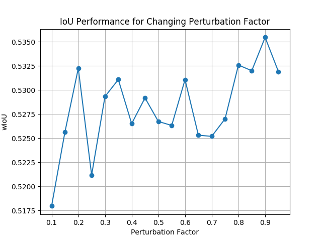
(a) Varying Perturbation Factor, $\uptau_{p}$

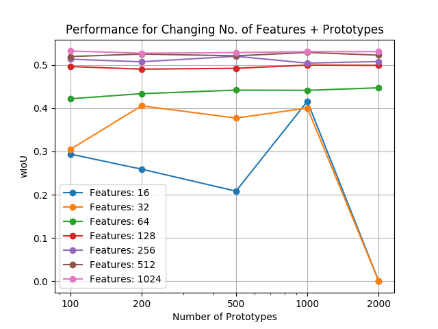
(b) Varying $D$ and $K$

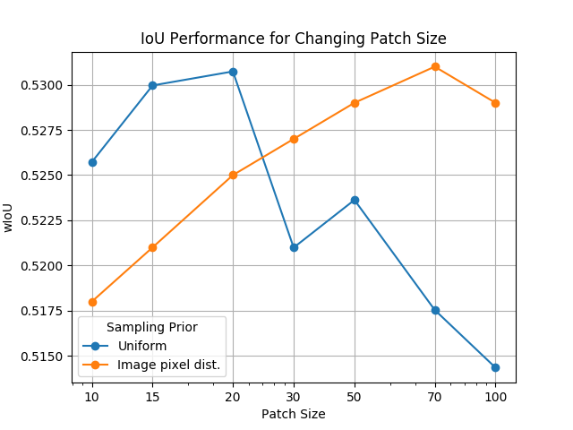
(c) Varying Patch Size, $M$

Figure 14: Effect of Varying Different Parameters on Segmentation Performance: Fig. (a) shows the variation in IoU performance for increasing perturbation factor $\uptau_{p}$ for image augmentation. Fig. (b) depicts the performance trends for varying image feature dimensions $D=|\textbf{Z}|$ and the number of prototype vectors $K=|\textbf{C}|$. Fig. (c) show the effects of increasing patch size on the segmentation IoU, both for a equiparitition constraint for SwAV clustering and a transport constraint based on the image pixel distribution.

Lastly, we present in Table 8 the effect of adding the local SwAV loss component to our contrastive loss on the overall IoU performance of our framework. From the table, we see that adding the local SwAV loss has a positive effect on the IoU performance for all the test classes.

Table 8: IoU Performance with and without local SwAV Loss: The table shows the effect of adding the local SwAV loss from Equation 10 on the overall wIoU performance of our framework.

Test Class	Face	Car	Cat	Horse
With Local SwAV Loss	53.61	18.53	18.57	8.96
W/o Local SwAV Loss	53.33	15.9	18.53	8.57

Table 9: Performance Comparison for Varying Configurations of the One-Shot segmenter: The table exhibits optimum performance in favor of lighter networks for one-shot segmentation.

Segmenter	Layers	wIoU	FG-IoU
MLP	1 layer	53.6	94.7
MLP	3 layers	53.1	94.1
FCN	3 layers	52.9	94.4
FCN	5 layers	52.7	93.9
FCN	7 layers	52.2	93.1
FCN	9 layers	52.1	92.9

9.3 One-Shot Segmentation

Table 9 compares $wIoU$ performance for varying configurations of the segmenter network. We see that using deeper networks also degrades the wIoU output for the framework which can be attributed to the overfitting of the additional parameters in the larger network.

Additionally, Table 10 studies the performance of the framework in a few-shot setting where it is compared to the supervised baseline from Table 3. While the growth of learning for our framework is similar to the semi-supervised baselines, we can see that it does catch up to supervised segmenter performance with as few as 10 training samples.

Table 10: IoU Performance for Our Framework in a Few-Shot Setting: The table compares the performance of the framework and other baselines against a supervised segmentation model when we increase the number of training samples fed to the few-shot segmenter.

Method	1-shot	5-shot	10-shot	Sup.
DatasetGAN	49.48	52.16	55.86	-
RepurposeGAN	51.46	60.86	63.71	-
HFC+KMeans	48.92	52.89	56.01	-
HFC+SimCLR	50.36	57.56	61.11	-
Ours	53.61	61.11	62.98	68.71

10 Conclusion

The paper has explored the utility of the hidden feature representations within GANs in building self-supervised learning models for one-shot segmentation. The proposed self-supervised approach for hidden feature clustering opens up new possibilities for utilizing the cluster representations for other downstream tasks pertaining to synthetic images. We also postulate that this approach can be extended to other generative models such as diffusion models by exploring the feature representations in their respective architectures.

Appendix A The Online Cluster Assignment Problem

As described in our paper, the computation of the swapped prediction loss for the SwAV model [8] requires the projection of image features Z onto a space spanned by learnable prototype vectors $\textbf{C}=\{\textbf{c}_{1},\textbf{c}_{2},\ldots,\textbf{c}_{K}\}$. The mapping $\textbf{C}^{T}\textbf{Z}$ is then used to obtain the encoding Q from which the cluster assignments are computed. For the SwAV model, the optimal encoding $\textbf{Q}^{*}$ is computed using the formulation in Asano . [3] where the cluster assignment problem is cast as an instance of the optimal transport equation as follows:

The SwAV model attempts to find an optimal $\textbf{Q}^{*}$ that maximizes the similarity between the cluster encoding Q and the mapped features $\textbf{C}^{T}\textbf{Z}$. This can be formulated as:

$$\textbf{Q}^{*} =\underset{\textbf{Q}\in\mathcal{Q}}{\arg\max}\>\>Tr(\textbf{Q}^{T}\textbf{C}^{T}\textbf{Z})$$

$$=\underset{\textbf{Q}\in\mathcal{Q}}{\arg\min}\left<\textbf{Q},-\textbf{C}^{T}\textbf{Z}\right>$$

To solve for Equation A, Asano . [3] begins by first enforcing an ‘equipartition constraint’ on Q. The intuition behind adding this constraint is to ensure that the batch of $B$ feature vectors are partitioned and mapped onto the prototypes equally. Hence, Q is restricted to the set of matrices whose row- and column-wise projections are probability distributions that split the data uniformly. The constraint is thus imposed as:

$$\textbf{Q}\in\mathcal{\bar{Q}}= \left\{\textbf{Q}\in\mathds{R}_{+}^{K\times B}\right.\>\>\big{|}\>\>$$ (13)

$$\>\>\left.\textbf{Q}\cdot\textbf{1}_{B}=\frac{1}{K}\textbf{1}_{K},\textbf{Q}^{T}\cdot\textbf{1}_{K}=\frac{1}{B}\textbf{1}_{B}\right\}$$

where K denotes the number of prototypes and $\textbf{1}_{x}$ are vectors consisting of all unit values. Definition of Q in this form ensures that each prototype $\textbf{c}_{i}$ is selected at least $B/K$ times in the batch. Because the rows and columns of Q are now essentially probability distributions, the Frobenius product in Equation A can be modeled as a version of the optimal transport problem [16]:

$$d_{M}(\textbf{r},\textbf{c})=\underset{\textbf{P}\in U(\textbf{r},\textbf{c})}{\min}\left<\textbf{P},\textbf{M}\right>$$ (14)

where the transport matrix P must be optimized to map a joint probability distribution r to another distribution c given the cost matrix M for r and c. In case of Equation A, Q becomes the transport matrix for optimization while $\textbf{C}^{T}\textbf{Z}$ denotes the cost matrix. Cuturi [16] proposes a closed-form solution to Equation 14 by adding a similarity constraint between P and $(\textbf{r},\textbf{c})$:

$$KL(\textbf{P}\>||\>\textbf{rc}^{T})\leq\lambda$$ (15)

where $KL(\cdot)$ is the Kullback-Liebler divergence. Since this expands to $H(\textbf{r})+H(\textbf{c})-H(\textbf{P})\leq\lambda$, the constrained optimization problem becomes:

$$d_{M}(\textbf{r},\textbf{c})=\underset{\textbf{P}\in U(\textbf{r,c})}{\arg\min}\left<\textbf{P, M}\right>-\frac{1}{\lambda}H(\textbf{P})$$ (16)

which is also referred to as the Sinkhorn distance. Equation 16 can be solved for P using Sinkhorn’s theorem [41] to obtain the following solution:

$$\textbf{P}=Diag(\textbf{u})\cdot e^{-\lambda\textbf{C}}\cdot Diag(\textbf{v})$$ (17)

where u and v are renormalization vectors that can be computed rapidly using the iterative Sinkhorn-Knopp algorithm [16].

Table 11: Training Configuration for our Framework for Different Test Classes: The table enlists the hyperparameter values configured for our framework for one-shot segmentation for the different test classes used in our experiments.

	Hyperparameter	Face	Car	Cat	Horse
Training	Object Labels	{background, skin, hair, eyebrow, nose, eye, mouth, ear}	{background, body, door, window, windshield, wheel,lights}	{background , head , eye , nose, ear , neck , torso , tail , f_leg , b_leg }	{ background , leg , saddle , torso , tail , head , rider }
	Epochs	100	100	100	50
	Number of Patches	5	5	5	10
	Perturbation Factor. $\uptau$	0.9	0.9	0.9	0.9
	Patch Size	20000	20000	20000	20000
Optimizer (SGD)	Learning Rate	0.01	0.01	0.01	0.01
	Momentum	0.9	0.9	0.9	0.9
	LARS Co-efficient, $t$	0.01	0.02	0.01	0.01
SwAV Loss	Temperature, $\tau$	0.01	0.01	0.02	0.02
	Number of Prototypes	5000	4000	5000	4000
	Number of Clusters	512	512	512	512
	Feature Dimension	5376	5888	5376	5376
	Sinkhorn Iterations	10	10	10	10
	Entropy Regularizer, $\lambda$	0.005	0.01	0.01	0.003

Reformulating Equation 16 for the SwAV loss,

$$\textbf{Q}^{*}=\underset{\textbf{Q}\in\mathcal{\bar{Q}}}{\arg\min}\left<\textbf{Q},-\textbf{C}^{T}\textbf{Z}\right>+\epsilon\cdot H(\textbf{Q})$$ (18)

the solution to the cluster assignment problem becomes:

$$\textbf{Q}^{*}=Diag(\textbf{u})\cdot\exp\left(\frac{\textbf{C}^{T}\textbf{Z}}{\upvarepsilon}\right)\cdot Diag(\textbf{v})$$ (19)

The advantage to using Sinkhorn distances is that the solution to the problem can be obtained in under as few as three iterations of the Sinkhorn-Knopp algorithm allowing a fast computation of cluster assignments. The SwAV method in our implementation uses this solution to learn and optimize the parameters for C and $\textbf{f}_{\theta}$ during training.

Appendix B Performance Evaluation and Comparison

This appendix expands upon the experiments and tests that we have presented in the paper to evaluate the performance of our work. These include the tests on one-shot segmentation, on boosting downstream computer vision tasks and for segmenting low-frequency object labels. What follows is a detailed breakdown of the experimental setup and results described in the paper for different test classes.

B.1 Setup and Training

Table 11 shows the training configuration of our framework for one-shot segmentation for each of the four test classes (Face, Car, Cat, Horse) described in the paper. The table enumerates the hyperparameters for data pre-processing and augmentation, the training optimizer and the SwAV loss formulation for each test class.

B.2 Segmentation Performance

In this section, we expand upon the one-shot segmentation results that were presented in our paper for the different test classes in Section 7.1 in the paper. The expanded results are depicted in Figs. 15 where IoU versus PD performance curves are obtained in the same manner as described in Section 7.2 in the paper. However, in this case, the curves are plotted for the individual object labels within each test class along with the mean IoU versus PD curve.

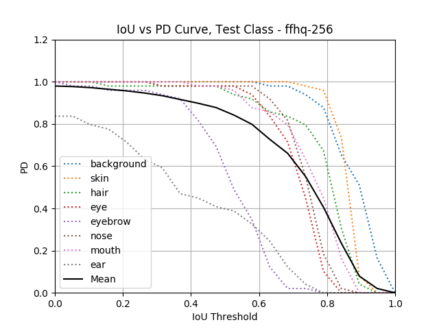
(a) Face Class

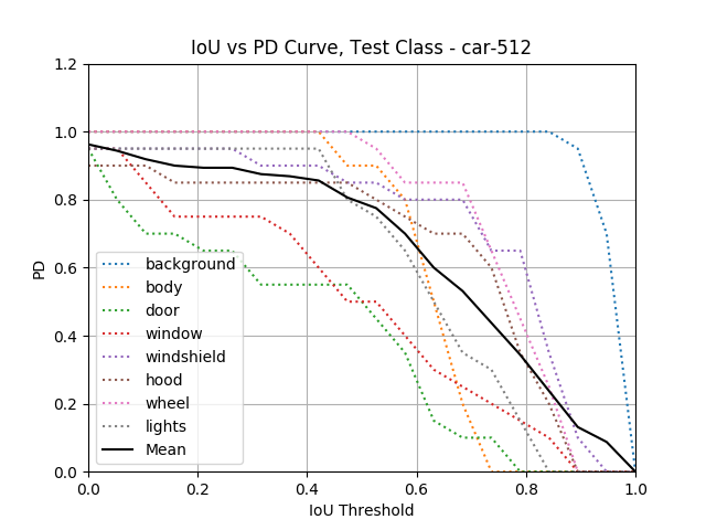
(b) Car Class

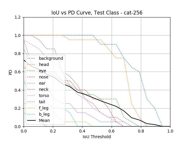
(c) Cat Class

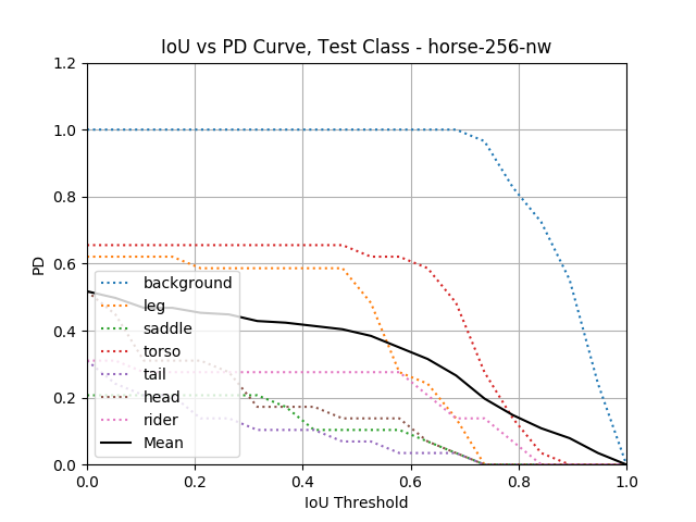
(d) Horse Class

Figure 15: Expanded mIoU versus PD Curves for One-Shot Segmentation: The plot shows the IoU versus PD performance curves for the different test classes where the curves are plotted individually for each object label in the test class.

Appendix C The BagGAN Framework

This appendix describes the design and implementation of the BagGAN framework where we have applied our proposed framework to labelled synthetic X-ray baggage scans for threat detection. The BagGAN framework is designed to produce realistic X-ray scans of checked baggage using StyleGANs while automatically extracting segmentation labels from the simulated images. It is constructed using a StyleGAN model pre-trained on the PIDRay baggage screening benchmark [43] and our proposed one- shot segmenter is then applied to the synthetic images to create new annotated samples for different threat items.

C.1 BagGAN Architecture and Training

As described in the paper, the BagGAN framework has been implemented for baggage simulation in two steps: (i) the first step includes pre-training a StyleGAN model for baggage image generation while (ii) the second step involves building the one-shot segmenter for automatic annotation of the generated images.

In our implementation, the BagGAN model comprises of a 7-layer generator and discriminator network whose architectural specification are provided in our code repository.

The model was trained using baggage X-ray scan samples from the PIDRay Baggage X-ray benchmark wherein each image sample is a top-view X-ray projection image of a scanned bag obtained from a two-view, dual-energy baggage screener. Every baggage image in the benchmark has a different dimension, hence, the training image data has been pre-processed by cropping the image samples to the dimensions $448\times 448\times 3$ and and resizing them to a dimension of $512\times 512\times 3$ for training the GAN.

The StyleGAN for our framework was trained with the image samples for 700 epochs to map a $512\times 1$ dimensional latent vector to a $512\times 512\times 3$ baggage image. During training, the adversarial loss was implemented with a Wasserstein loss weighted at $\lambda_{wgan}=0.5$ and a gradient penalty term (with $\lambda_{gp}=0.5$) was added to maintain the Lipschitz constraints. For latent space smoothing, a PPL (Perceptual Path Length) regularizer was added to the loss with the following hyperparameters: $\{\lambda_{ppl}=2,iter_{ppl,d}=16,iter_{ppl,g}=4,r_{ppl-decay}=0.01,batch_{ppl,shrink}=2\}$.

The following R1 regularization term was also added for stability by penalizing the adversarial loss gradient $\lvert\lvert\textbf{D}(\textbf{x})\lvert\lvert^{2}$ for the real data x alone:

$$R_{1}(\theta)=\frac{\gamma}{2}\mathds{E}_{D(\textbf{x})}\left[\lvert\lvert\textbf{D}_{\theta}(\textbf{x})\lvert\lvert^{2}\right]$$ (20)

Additionally, style mixing regularization was performed where two different sampled latent vectors were mixed before being fed to the image synthesis blocks.

To avoid discriminator overfitting, adaptive discriminator augmentation [25] was also applied. For augmentation, the baggage images were transformed using random recoloring and rotations. The following hyperparameters were used for ADA: target augmentation probability $(t_{ada}=0.6)$, probability update interval $(iter_{ada}=8)$, length for augmentation probablilty $(l_{ada}=5\times 10^{5})$.

The training error curves for the model as well as the trends in image fidelity (FID) during training are plotted in Fig. 16.

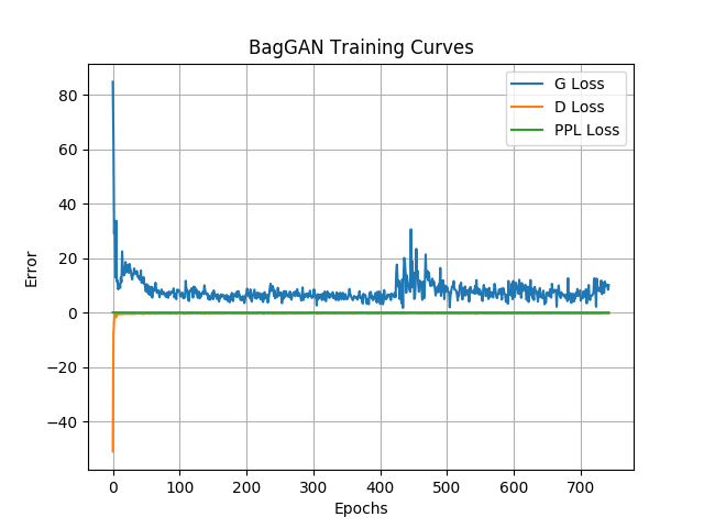
(a)

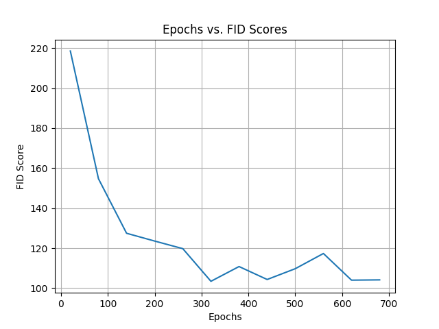
(b)

Figure 16: Training Curves for the BagGAN Framework: The figure shows (i) Training Error curves for the BagGAN model for StyleGAN2-ADA Pre- training and (ii) the trends in FID Scores for the StyleGAN2 model during training.

C.2 Simulation Results

Examples of baggage X-ray images generated using the trained model for different threat categories are illustrated in Fig. 17. These generated images have been used in our experiments in the paper to evaluate the performance of the BagGAN framework. Additionally, we have also shown in Fig. 18 a comparison of the simulated baggage images obtained from BagGAN with the X-ray images generated using a traditional, physics-based X-ray image simulator [35]. A visual comparison between the two sets of simulated images demonstrates how faithfully our framework is able to replicate the diversity and structure of the scanned baggage images from the PIDRay dataset.

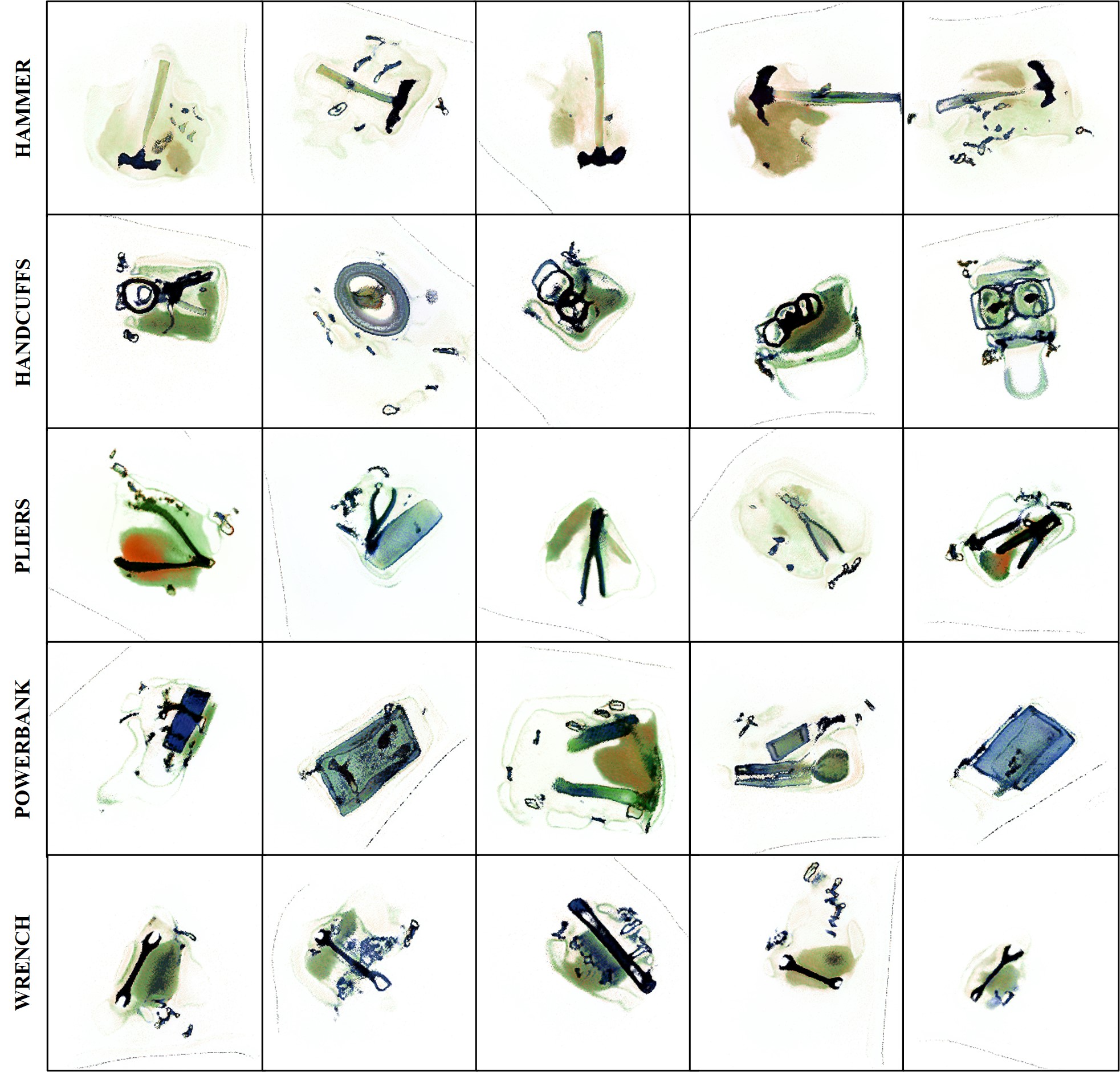
Figure 17: Examples of Baggage X-ray images from BagGAN: The images were generated by the trained StyleGAN model in BagGAN for 5 different threat item categories (hammer, handcuffs, pliers, powerbank, wrench).

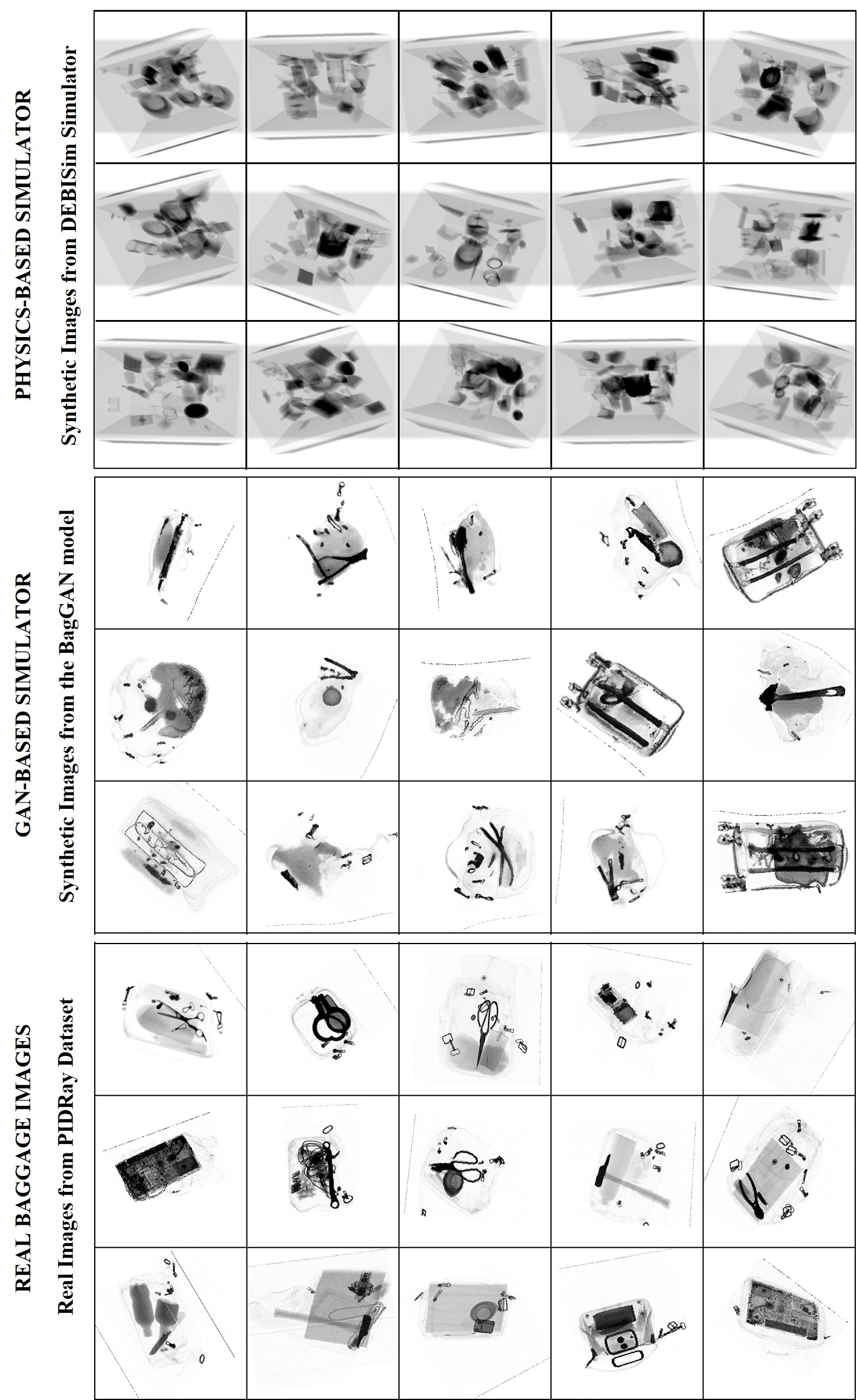
Figure 18: Comparison between Physics-based and GAN-based Simulators: The first collage depicts simulated baggage scans from a physics-based X-ray simulator (DEBISim -[35]). The second collage shows images produced by a StyleGAN trained on a baggage screening dataset. The last collage shows real baggage scans from the same dataset [43]. Note: The comparison shows the baggage images in grayscale for better visual comparison but the BagGAN and PIDRay images are actually pseudo-colored as shown in Fig. 17.

References

- \bibcommenthead
- Abdal \BOthers. [\APACyear2019] \APACinsertmetastarabdal2019image2stylegan{APACrefauthors}Abdal, R., Qin, Y.\BCBL Wonka, P. \APACrefYearMonthDay2019. \BBOQ\APACrefatitleImage2stylegan: How to embed images into the stylegan latent space? Image2stylegan: How to embed images into the stylegan latent space?\BBCQ \APACrefbtitleProceedings of the IEEE/CVF International Conference on Computer Vision Proceedings of the ieee/cvf international conference on computer vision (\BPGS 4432–4441). \PrintBackRefs\CurrentBib
- Abdal \BOthers. [\APACyear2021] \APACinsertmetastarabdal2021labels4free{APACrefauthors}Abdal, R., Zhu, P., Mitra, N.\BCBL Wonka, P. \APACrefYearMonthDay2021. \BBOQ\APACrefatitleLabels4Free: Unsupervised Segmentation using StyleGAN Labels4free: Unsupervised segmentation using stylegan.\BBCQ \APACjournalVolNumPagesarXiv preprint arXiv:2103.14968, \PrintBackRefs\CurrentBib
- Asano \BOthers. [\APACyear2019] \APACinsertmetastarasano2019self{APACrefauthors}Asano, Y.M., Rupprecht, C.\BCBL Vedaldi, A. \APACrefYearMonthDay2019. \BBOQ\APACrefatitleSelf-labelling via simultaneous clustering and representation learning Self-labelling via simultaneous clustering and representation learning.\BBCQ \APACjournalVolNumPagesarXiv preprint arXiv:1911.05371, \PrintBackRefs\CurrentBib
- Bengio \BOthers. [\APACyear2003] \APACinsertmetastarbengio2003neural{APACrefauthors}Bengio, Y., Ducharme, R., Vincent, P.\BCBL Jauvin, C. \APACrefYearMonthDay2003. \BBOQ\APACrefatitleA Neural Probabilistic Language Model A neural probabilistic language model.\BBCQ \APACjournalVolNumPagesJournal of Machine Learning Research31137–1155, \PrintBackRefs\CurrentBib
- Benny \BBA Wolf [\APACyear2020] \APACinsertmetastarbenny2020onegan{APACrefauthors}Benny, Y.\BCBT \BBA Wolf, L. \APACrefYearMonthDay2020. \BBOQ\APACrefatitleOnegan: Simultaneous unsupervised learning of conditional image generation, foreground segmentation, and fine-grained clustering Onegan: Simultaneous unsupervised learning of conditional image generation, foreground segmentation, and fine-grained clustering.\BBCQ \APACrefbtitleEuropean Conference on Computer Vision European conference on computer vision (\BPGS 514–530). \PrintBackRefs\CurrentBib
- Bond-Taylor \BOthers. [\APACyear2021] \APACinsertmetastarbond2021deep{APACrefauthors}Bond-Taylor, S., Leach, A., Long, Y.\BCBL Willcocks, C.G. \APACrefYearMonthDay2021. \BBOQ\APACrefatitleDeep generative modelling: A comparative review of vaes, gans, normalizing flows, energy-based and autoregressive models Deep generative modelling: A comparative review of vaes, gans, normalizing flows, energy-based and autoregressive models.\BBCQ \APACjournalVolNumPagesarXiv preprint arXiv:2103.04922, \PrintBackRefs\CurrentBib
- Caron \BOthers. [\APACyear2018] \APACinsertmetastarcaron2018deep{APACrefauthors}Caron, M., Bojanowski, P., Joulin, A.\BCBL Douze, M. \APACrefYearMonthDay2018. \BBOQ\APACrefatitleDeep clustering for unsupervised learning of visual features Deep clustering for unsupervised learning of visual features.\BBCQ \APACrefbtitleProceedings of the European conference on computer vision (ECCV) Proceedings of the european conference on computer vision (eccv) (\BPGS 132–149). \PrintBackRefs\CurrentBib
- Caron \BOthers. [\APACyear2020] \APACinsertmetastarcaron2020unsupervised{APACrefauthors}Caron, M., Misra, I., Mairal, J., Goyal, P., Bojanowski, P.\BCBL Joulin, A. \APACrefYearMonthDay2020. \BBOQ\APACrefatitleUnsupervised learning of visual features by contrasting cluster assignments Unsupervised learning of visual features by contrasting cluster assignments.\BBCQ \APACjournalVolNumPagesAdvances in Neural Information Processing Systems339912–9924, \PrintBackRefs\CurrentBib
- Chaitanya \BOthers. [\APACyear2020] \APACinsertmetastarchaitanya2020contrastive{APACrefauthors}Chaitanya, K., Erdil, E., Karani, N.\BCBL Konukoglu, E. \APACrefYearMonthDay2020. \BBOQ\APACrefatitleContrastive learning of global and local features for medical image segmentation with limited annotations Contrastive learning of global and local features for medical image segmentation with limited annotations.\BBCQ \APACjournalVolNumPagesAdvances in Neural Information Processing Systems3312546–12558, \PrintBackRefs\CurrentBib
- L\BHBIC. Chen \BOthers. [\APACyear2017] \APACinsertmetastarchen2017rethinking{APACrefauthors}Chen, L\BHBIC., Papandreou, G., Schroff, F.\BCBL Adam, H. \APACrefYearMonthDay2017. \BBOQ\APACrefatitleRethinking atrous convolution for semantic image segmentation Rethinking atrous convolution for semantic image segmentation.\BBCQ \APACjournalVolNumPagesarXiv preprint arXiv:1706.05587, \PrintBackRefs\CurrentBib
- T. Chen, Kornblith, Norouzi\BCBL \BBA Hinton [\APACyear2020] \APACinsertmetastarchen2020simple{APACrefauthors}Chen, T., Kornblith, S., Norouzi, M.\BCBL Hinton, G. \APACrefYearMonthDay2020. \BBOQ\APACrefatitleA simple framework for contrastive learning of visual representations A simple framework for contrastive learning of visual representations.\BBCQ \APACrefbtitleInternational conference on machine learning International conference on machine learning (\BPGS 1597–1607). \PrintBackRefs\CurrentBib
- T. Chen, Kornblith, Swersky\BCBL \BOthers. [\APACyear2020] \APACinsertmetastarchen2020big{APACrefauthors}Chen, T., Kornblith, S., Swersky, K., Norouzi, M.\BCBL Hinton, G.E. \APACrefYearMonthDay2020. \BBOQ\APACrefatitleBig self-supervised models are strong semi-supervised learners Big self-supervised models are strong semi-supervised learners.\BBCQ \APACjournalVolNumPagesAdvances in neural information processing systems3322243–22255, \PrintBackRefs\CurrentBib
- X. Chen \BOthers. [\APACyear2014] \APACinsertmetastarchen2014detect{APACrefauthors}Chen, X., Mottaghi, R., Liu, X., Fidler, S., Urtasun, R.\BCBL Yuille, A. \APACrefYearMonthDay2014. \BBOQ\APACrefatitleDetect what you can: Detecting and representing objects using holistic models and body parts Detect what you can: Detecting and representing objects using holistic models and body parts.\BBCQ \APACrefbtitleProceedings of the IEEE conference on computer vision and pattern recognition Proceedings of the ieee conference on computer vision and pattern recognition (\BPGS 1971–1978). \PrintBackRefs\CurrentBib
- Cheng \BOthers. [\APACyear2021] \APACinsertmetastarcheng2021out{APACrefauthors}Cheng, Y\BHBIC., Lin, C.H., Lee, H\BHBIY., Ren, J., Tulyakov, S.\BCBL Yang, M\BHBIH. \APACrefYearMonthDay2021. \BBOQ\APACrefatitleIn&out: Diverse image outpainting via gan inversion In&out: Diverse image outpainting via gan inversion.\BBCQ \APACjournalVolNumPagesarXiv preprint arXiv:2104.00675, \PrintBackRefs\CurrentBib
- Choi \BOthers. [\APACyear2020] \APACinsertmetastarchoi2020starganv2{APACrefauthors}Choi, Y., Uh, Y., Yoo, J.\BCBL Ha, J\BHBIW. \APACrefYearMonthDay2020. \BBOQ\APACrefatitleStarGAN v2: Diverse Image Synthesis for Multiple Domains Stargan v2: Diverse image synthesis for multiple domains.\BBCQ \APACrefbtitleProceedings of the IEEE Conference on Computer Vision and Pattern Recognition. Proceedings of the ieee conference on computer vision and pattern recognition. \PrintBackRefs\CurrentBib
- Cuturi [\APACyear2013] \APACinsertmetastarcuturi2013sinkhorn{APACrefauthors}Cuturi, M. \APACrefYearMonthDay2013. \BBOQ\APACrefatitleSinkhorn distances: Lightspeed computation of optimal transport Sinkhorn distances: Lightspeed computation of optimal transport.\BBCQ \APACjournalVolNumPagesAdvances in neural information processing systems26, \PrintBackRefs\CurrentBib
- Dhariwal \BBA Nichol [\APACyear2021] \APACinsertmetastardhariwal2021diffusion{APACrefauthors}Dhariwal, P.\BCBT \BBA Nichol, A. \APACrefYearMonthDay2021. \BBOQ\APACrefatitleDiffusion models beat gans on image synthesis Diffusion models beat gans on image synthesis.\BBCQ \APACjournalVolNumPagesAdvances in Neural Information Processing Systems34, \PrintBackRefs\CurrentBib
- Dong \BBA Xing [\APACyear2018] \APACinsertmetastardong2018few{APACrefauthors}Dong, N.\BCBT \BBA Xing, E.P. \APACrefYearMonthDay2018. \BBOQ\APACrefatitleFew-shot semantic segmentation with prototype learning. Few-shot semantic segmentation with prototype learning.\BBCQ \APACrefbtitleBMVC Bmvc (\BVOL 3). \PrintBackRefs\CurrentBib
- Gidaris \BOthers. [\APACyear2018] \APACinsertmetastargidaris2018unsupervised{APACrefauthors}Gidaris, S., Singh, P.\BCBL Komodakis, N. \APACrefYearMonthDay2018. \BBOQ\APACrefatitleUnsupervised Representation Learning by Predicting Image Rotations Unsupervised representation learning by predicting image rotations.\BBCQ \APACrefbtitleInternational Conference on Learning Representations. International conference on learning representations. \PrintBackRefs\CurrentBib
- Goodfellow \BOthers. [\APACyear2014] \APACinsertmetastargoodfellow2014generative{APACrefauthors}Goodfellow, I., Pouget-Abadie, J., Mirza, M., Xu, B., Warde-Farley, D., Ozair, S.\BDBLBengio, Y. \APACrefYearMonthDay2014. \BBOQ\APACrefatitleGenerative adversarial nets Generative adversarial nets.\BBCQ \APACjournalVolNumPagesAdvances in neural information processing systems27, \PrintBackRefs\CurrentBib
- Higgins \BOthers. [\APACyear2018] \APACinsertmetastarhiggins2018towards{APACrefauthors}Higgins, I., Amos, D., Pfau, D., Racaniere, S., Matthey, L., Rezende, D.\BCBL Lerchner, A. \APACrefYearMonthDay2018. \BBOQ\APACrefatitleTowards a definition of disentangled representations Towards a definition of disentangled representations.\BBCQ \APACjournalVolNumPagesarXiv preprint arXiv:1812.02230, \PrintBackRefs\CurrentBib
- Huang \BBA Belongie [\APACyear2017] \APACinsertmetastarhuang2017arbitrary{APACrefauthors}Huang, X.\BCBT \BBA Belongie, S. \APACrefYearMonthDay2017. \BBOQ\APACrefatitleArbitrary style transfer in real-time with adaptive instance normalization Arbitrary style transfer in real-time with adaptive instance normalization.\BBCQ \APACrefbtitleProceedings of the IEEE international conference on computer vision Proceedings of the ieee international conference on computer vision (\BPGS 1501–1510). \PrintBackRefs\CurrentBib
- Hung \BOthers. [\APACyear2019] \APACinsertmetastarhung2019scops{APACrefauthors}Hung, W\BHBIC., Jampani, V., Liu, S., Molchanov, P., Yang, M\BHBIH.\BCBL Kautz, J. \APACrefYearMonthDay2019. \BBOQ\APACrefatitleScops: Self-supervised co-part segmentation Scops: Self-supervised co-part segmentation.\BBCQ \APACrefbtitleProceedings of the IEEE/CVF Conference on Computer Vision and Pattern Recognition Proceedings of the ieee/cvf conference on computer vision and pattern recognition (\BPGS 869–878). \PrintBackRefs\CurrentBib
- Jing \BBA Tian [\APACyear2020] \APACinsertmetastarjing2020self{APACrefauthors}Jing, L.\BCBT \BBA Tian, Y. \APACrefYearMonthDay2020. \BBOQ\APACrefatitleSelf-supervised visual feature learning with deep neural networks: A survey Self-supervised visual feature learning with deep neural networks: A survey.\BBCQ \APACjournalVolNumPagesIEEE transactions on pattern analysis and machine intelligence43114037–4058, \PrintBackRefs\CurrentBib
- Karras, Aittala\BCBL \BOthers. [\APACyear2020] \APACinsertmetastarkarras2020training{APACrefauthors}Karras, T., Aittala, M., Hellsten, J., Laine, S., Lehtinen, J.\BCBL Aila, T. \APACrefYearMonthDay2020. \BBOQ\APACrefatitleTraining generative adversarial networks with limited data Training generative adversarial networks with limited data.\BBCQ \APACjournalVolNumPagesarXiv preprint arXiv:2006.06676, \PrintBackRefs\CurrentBib
- Karras \BOthers. [\APACyear2019] \APACinsertmetastarkarras2019style{APACrefauthors}Karras, T., Laine, S.\BCBL Aila, T. \APACrefYearMonthDay2019. \BBOQ\APACrefatitleA style-based generator architecture for generative adversarial networks A style-based generator architecture for generative adversarial networks.\BBCQ \APACrefbtitleProceedings of the IEEE/CVF Conference on Computer Vision and Pattern Recognition Proceedings of the ieee/cvf conference on computer vision and pattern recognition (\BPGS 4401–4410). \PrintBackRefs\CurrentBib
- Karras, Laine\BCBL \BOthers. [\APACyear2020] \APACinsertmetastarkarras2020analyzing{APACrefauthors}Karras, T., Laine, S., Aittala, M., Hellsten, J., Lehtinen, J.\BCBL Aila, T. \APACrefYearMonthDay2020. \BBOQ\APACrefatitleAnalyzing and improving the image quality of stylegan Analyzing and improving the image quality of stylegan.\BBCQ \APACrefbtitleProceedings of the IEEE/CVF Conference on Computer Vision and Pattern Recognition Proceedings of the ieee/cvf conference on computer vision and pattern recognition (\BPGS 8110–8119). \PrintBackRefs\CurrentBib
- Kingma \BBA Welling [\APACyear2013] \APACinsertmetastarkingma2013auto{APACrefauthors}Kingma, D.P.\BCBT \BBA Welling, M. \APACrefYearMonthDay2013. \BBOQ\APACrefatitleAuto-encoding variational bayes Auto-encoding variational bayes.\BBCQ \APACjournalVolNumPagesarXiv preprint arXiv:1312.6114, \PrintBackRefs\CurrentBib
- Lee \BOthers. [\APACyear2020] \APACinsertmetastarlee2020maskgan{APACrefauthors}Lee, C\BHBIH., Liu, Z., Wu, L.\BCBL Luo, P. \APACrefYearMonthDay2020. \BBOQ\APACrefatitleMaskGAN: Towards Diverse and Interactive Facial Image Manipulation Maskgan: Towards diverse and interactive facial image manipulation.\BBCQ \APACrefbtitleIEEE Conference on Computer Vision and Pattern Recognition (CVPR). Ieee conference on computer vision and pattern recognition (cvpr). \PrintBackRefs\CurrentBib
- Le-Khac \BOthers. [\APACyear2020] \APACinsertmetastarle2020contrastive{APACrefauthors}Le-Khac, P.H., Healy, G.\BCBL Smeaton, A.F. \APACrefYearMonthDay2020. \BBOQ\APACrefatitleContrastive representation learning: A framework and review Contrastive representation learning: A framework and review.\BBCQ \APACjournalVolNumPagesIEEE Access8193907–193934, \PrintBackRefs\CurrentBib
- Li \BOthers. [\APACyear2021] \APACinsertmetastarli2021semantic{APACrefauthors}Li, D., Yang, J., Kreis, K., Torralba, A.\BCBL Fidler, S. \APACrefYearMonthDay2021. \BBOQ\APACrefatitleSemantic segmentation with generative models: Semi-supervised learning and strong out-of-domain generalization Semantic segmentation with generative models: Semi-supervised learning and strong out-of-domain generalization.\BBCQ \APACrefbtitleProceedings of the IEEE/CVF Conference on Computer Vision and Pattern Recognition Proceedings of the ieee/cvf conference on computer vision and pattern recognition (\BPGS 8300–8311). \PrintBackRefs\CurrentBib
- Ling \BOthers. [\APACyear2021] \APACinsertmetastarling2021editgan{APACrefauthors}Ling, H., Kreis, K., Li, D., Kim, S.W., Torralba, A.\BCBL Fidler, S. \APACrefYearMonthDay2021. \BBOQ\APACrefatitleEditGAN: High-Precision Semantic Image Editing Editgan: High-precision semantic image editing.\BBCQ \APACjournalVolNumPagesAdvances in Neural Information Processing Systems34, \PrintBackRefs\CurrentBib
- X. Liu \BOthers. [\APACyear2021] \APACinsertmetastarliu2021self{APACrefauthors}Liu, X., Zhang, F., Hou, Z., Mian, L., Wang, Z., Zhang, J.\BCBL Tang, J. \APACrefYearMonthDay2021. \BBOQ\APACrefatitleSelf-supervised learning: Generative or contrastive Self-supervised learning: Generative or contrastive.\BBCQ \APACjournalVolNumPagesIEEE Transactions on Knowledge and Data Engineering, \PrintBackRefs\CurrentBib
- Z. Liu \BOthers. [\APACyear2018] \APACinsertmetastarliu2018large{APACrefauthors}Liu, Z., Luo, P., Wang, X.\BCBL Tang, X. \APACrefYearMonthDay2018. \BBOQ\APACrefatitleLarge-scale celebfaces attributes (celeba) dataset Large-scale celebfaces attributes (celeba) dataset.\BBCQ \APACjournalVolNumPagesRetrieved August15201811, \PrintBackRefs\CurrentBib
- Manerikar \BOthers. [\APACyear2021] \APACinsertmetastarmanerikar2021debisim{APACrefauthors}Manerikar, A., Li, F.\BCBL Kak, A.C. \APACrefYearMonthDay2021. \BBOQ\APACrefatitleDEBISim: A simulation pipeline for dual energy CT-based baggage inspection systems Debisim: A simulation pipeline for dual energy ct-based baggage inspection systems.\BBCQ \APACjournalVolNumPagesJournal of X-ray science and technology292259–285, \PrintBackRefs\CurrentBib
- Manerikar \BOthers. [\APACyear2020] \APACinsertmetastarmanerikar2020adaptive{APACrefauthors}Manerikar, A., Prakash, T.\BCBL Kak, A.C. \APACrefYearMonthDay2020. \BBOQ\APACrefatitleAdaptive target recognition: A case study involving airport baggage screening Adaptive target recognition: A case study involving airport baggage screening.\BBCQ \APACrefbtitleAnomaly Detection and Imaging with X-Rays (ADIX) V Anomaly detection and imaging with x-rays (adix) v (\BVOL 11404, \BPGS 12–24). \PrintBackRefs\CurrentBib
- Pakhomov \BOthers. [\APACyear2021] \APACinsertmetastarpakhomov2021segmentation{APACrefauthors}Pakhomov, D., Hira, S., Wagle, N., Green, K.E.\BCBL Navab, N. \APACrefYearMonthDay2021. \BBOQ\APACrefatitleSegmentation in style: Unsupervised semantic image segmentation with stylegan and clip Segmentation in style: Unsupervised semantic image segmentation with stylegan and clip.\BBCQ \APACjournalVolNumPagesarXiv preprint arXiv:2107.12518, \PrintBackRefs\CurrentBib
- Pathak \BOthers. [\APACyear2016] \APACinsertmetastarpathak2016context{APACrefauthors}Pathak, D., Krahenbuhl, P., Donahue, J., Darrell, T.\BCBL Efros, A.A. \APACrefYearMonthDay2016. \BBOQ\APACrefatitleContext encoders: Feature learning by inpainting Context encoders: Feature learning by inpainting.\BBCQ \APACrefbtitleProceedings of the IEEE conference on computer vision and pattern recognition Proceedings of the ieee conference on computer vision and pattern recognition (\BPGS 2536–2544). \PrintBackRefs\CurrentBib
- Richardson \BOthers. [\APACyear2021] \APACinsertmetastarrichardson2021encoding{APACrefauthors}Richardson, E., Alaluf, Y., Patashnik, O., Nitzan, Y., Azar, Y., Shapiro, S.\BCBL Cohen-Or, D. \APACrefYearMonthDay2021. \BBOQ\APACrefatitleEncoding in style: a stylegan encoder for image-to-image translation Encoding in style: a stylegan encoder for image-to-image translation.\BBCQ \APACrefbtitleProceedings of the IEEE/CVF Conference on Computer Vision and Pattern Recognition Proceedings of the ieee/cvf conference on computer vision and pattern recognition (\BPGS 2287–2296). \PrintBackRefs\CurrentBib
- Shoshan \BOthers. [\APACyear2021] \APACinsertmetastarshoshan2021gan{APACrefauthors}Shoshan, A., Bhonker, N., Kviatkovsky, I.\BCBL Medioni, G. \APACrefYearMonthDay2021. \BBOQ\APACrefatitleGan-control: Explicitly controllable gans Gan-control: Explicitly controllable gans.\BBCQ \APACrefbtitleProceedings of the IEEE/CVF International Conference on Computer Vision Proceedings of the ieee/cvf international conference on computer vision (\BPGS 14083–14093). \PrintBackRefs\CurrentBib
- Sinkhorn \BBA Knopp [\APACyear1967] \APACinsertmetastarsinkhorn1967concerning{APACrefauthors}Sinkhorn, R.\BCBT \BBA Knopp, P. \APACrefYearMonthDay1967. \BBOQ\APACrefatitleConcerning nonnegative matrices and doubly stochastic matrices Concerning nonnegative matrices and doubly stochastic matrices.\BBCQ \APACjournalVolNumPagesPacific Journal of Mathematics212343–348, \PrintBackRefs\CurrentBib
- Tritrong \BOthers. [\APACyear2021] \APACinsertmetastartritrong2021repurposing{APACrefauthors}Tritrong, N., Rewatbowornwong, P.\BCBL Suwajanakorn, S. \APACrefYearMonthDay2021. \BBOQ\APACrefatitleRepurposing gans for one-shot semantic part segmentation Repurposing gans for one-shot semantic part segmentation.\BBCQ \APACrefbtitleProceedings of the IEEE/CVF Conference on Computer Vision and Pattern Recognition Proceedings of the ieee/cvf conference on computer vision and pattern recognition (\BPGS 4475–4485). \PrintBackRefs\CurrentBib
- Wang \BOthers. [\APACyear2021] \APACinsertmetastarwang2021towards{APACrefauthors}Wang, B., Zhang, L., Wen, L., Liu, X.\BCBL Wu, Y. \APACrefYearMonthDay2021. \BBOQ\APACrefatitleTowards Real-World Prohibited Item Detection: A Large-Scale X-ray Benchmark Towards real-world prohibited item detection: A large-scale x-ray benchmark.\BBCQ \APACrefbtitleProceedings of the IEEE/CVF International Conference on Computer Vision Proceedings of the ieee/cvf international conference on computer vision (\BPGS 5412–5421). \PrintBackRefs\CurrentBib
- Yang \BOthers. [\APACyear2022] \APACinsertmetastaryang2022learning{APACrefauthors}Yang, Y., Bilen, H., Zou, Q., Cheung, W.Y.\BCBL Ji, X. \APACrefYearMonthDay2022. \BBOQ\APACrefatitleLearning Foreground-Background Segmentation from Improved Layered GANs Learning foreground-background segmentation from improved layered gans.\BBCQ \APACrefbtitleProceedings of the IEEE/CVF Winter Conference on Applications of Computer Vision Proceedings of the ieee/cvf winter conference on applications of computer vision (\BPGS 2524–2533). \PrintBackRefs\CurrentBib
- Yang \BOthers. [\APACyear2021] \APACinsertmetastaryang2021learning{APACrefauthors}Yang, Y., Cheng, X., Bilen, H.\BCBL Ji, X. \APACrefYearMonthDay2021. \BBOQ\APACrefatitleLearning to Annotate Part Segmentation with Gradient Matching Learning to annotate part segmentation with gradient matching.\BBCQ \APACrefbtitleInternational Conference on Learning Representations. International conference on learning representations. \PrintBackRefs\CurrentBib
- You \BOthers. [\APACyear2017] \APACinsertmetastaryou2017large{APACrefauthors}You, Y., Gitman, I.\BCBL Ginsburg, B. \APACrefYearMonthDay2017. \BBOQ\APACrefatitleLarge batch training of convolutional networks Large batch training of convolutional networks.\BBCQ \APACjournalVolNumPagesarXiv preprint arXiv:1708.03888, \PrintBackRefs\CurrentBib
- Yu, Seff\BCBL \BOthers. [\APACyear2015] \APACinsertmetastaryu2015lsun{APACrefauthors}Yu, F., Seff, A., Zhang, Y., Song, S., Funkhouser, T.\BCBL Xiao, J. \APACrefYearMonthDay2015. \BBOQ\APACrefatitleLsun: Construction of a large-scale image dataset using deep learning with humans in the loop Lsun: Construction of a large-scale image dataset using deep learning with humans in the loop.\BBCQ \APACjournalVolNumPagesarXiv preprint arXiv:1506.03365, \PrintBackRefs\CurrentBib
- Yu, Zhang\BCBL \BOthers. [\APACyear2015] \APACinsertmetastaryu15lsun{APACrefauthors}Yu, F., Zhang, Y., Song, S., Seff, A.\BCBL Xiao, J. \APACrefYearMonthDay2015. \BBOQ\APACrefatitleLSUN: Construction of a Large-scale Image Dataset using Deep Learning with Humans in the Loop Lsun: Construction of a large-scale image dataset using deep learning with humans in the loop.\BBCQ \APACjournalVolNumPagesarXiv preprint arXiv:1506.03365, \PrintBackRefs\CurrentBib
- C. Zhang \BOthers. [\APACyear2019] \APACinsertmetastarzhang2019canet{APACrefauthors}Zhang, C., Lin, G., Liu, F., Yao, R.\BCBL Shen, C. \APACrefYearMonthDay2019. \BBOQ\APACrefatitleCanet: Class-agnostic segmentation networks with iterative refinement and attentive few-shot learning Canet: Class-agnostic segmentation networks with iterative refinement and attentive few-shot learning.\BBCQ \APACrefbtitleProceedings of the IEEE/CVF Conference on Computer Vision and Pattern Recognition Proceedings of the ieee/cvf conference on computer vision and pattern recognition (\BPGS 5217–5226). \PrintBackRefs\CurrentBib
- X. Zhang \BOthers. [\APACyear2020] \APACinsertmetastarzhang2020sg{APACrefauthors}Zhang, X., Wei, Y., Yang, Y.\BCBL Huang, T.S. \APACrefYearMonthDay2020. \BBOQ\APACrefatitleSg-one: Similarity guidance network for one-shot semantic segmentation Sg-one: Similarity guidance network for one-shot semantic segmentation.\BBCQ \APACjournalVolNumPagesIEEE Transactions on Cybernetics5093855–3865, \PrintBackRefs\CurrentBib
- Y. Zhang \BOthers. [\APACyear2021] \APACinsertmetastarzhang2021datasetgan{APACrefauthors}Zhang, Y., Ling, H., Gao, J., Yin, K., Lafleche, J\BHBIF., Barriuso, A.\BDBLFidler, S. \APACrefYearMonthDay2021. \BBOQ\APACrefatitleDatasetgan: Efficient labeled data factory with minimal human effort Datasetgan: Efficient labeled data factory with minimal human effort.\BBCQ \APACrefbtitleProceedings of the IEEE/CVF Conference on Computer Vision and Pattern Recognition Proceedings of the ieee/cvf conference on computer vision and pattern recognition (\BPGS 10145–10155). \PrintBackRefs\CurrentBib
- Zhao \BOthers. [\APACyear2017] \APACinsertmetastarzhao2017learning{APACrefauthors}Zhao, S., Song, J.\BCBL Ermon, S. \APACrefYearMonthDay2017. \BBOQ\APACrefatitleLearning hierarchical features from deep generative models Learning hierarchical features from deep generative models.\BBCQ \APACrefbtitleInternational Conference on Machine Learning International conference on machine learning (\BPGS 4091–4099). \PrintBackRefs\CurrentBib
- Ziegler \BBA Asano [\APACyear2022] \APACinsertmetastarziegler2022self{APACrefauthors}Ziegler, A.\BCBT \BBA Asano, Y.M. \APACrefYearMonthDay2022. \BBOQ\APACrefatitleSelf-Supervised Learning of Object Parts for Semantic Segmentation Self-supervised learning of object parts for semantic segmentation.\BBCQ \APACrefbtitleProceedings of the IEEE/CVF Conference on Computer Vision and Pattern Recognition Proceedings of the ieee/cvf conference on computer vision and pattern recognition (\BPGS 14502–14511). \PrintBackRefs\CurrentBib