Discrete-Time Mean-Field Stochastic Control with Partial Observations

Abstract

We study the optimal control of discrete time mean filed dynamical systems under partial observations. We express the global law of the filtered process as a controlled system with its own dynamics. Following a dynamic programming approach, we prove a verification result providing a solution to the optimal control of the filtered system. As an application, we study a general linear quadratic example for which an explicit solution is given. We also describe an algorithm for the numerical approximation of the optimal value and provide numerical experiments on a financial example.

MSC Classification: 60K35, 60G35, 49L20.

Keywords: Optimal control, mean-field interaction, partial observation, dynamic programming.

1 Introduction

We consider an optimal control problem for a system with mean field discrete time dynamics under partial observations. The question of how to optimally control a system with mean field dependence in the dynamics is related to the modelization of the optimal behavior for populations with large number of interacting individuals.

The case where each individual chooses an own action in order to optimise a non-cooperative reward, has led to the theory of mean-field games (MFGs), introduced in [12] and [13]. The Nash equilibrium is then described by two equations, the first one corresponding to the optimal behavior of a representative agent and the second one corresponding to the evolution of the whole population under the optimal choice of each individual.

In the case where all the individuals follow the same goal, the cooperative behavior leads to the optimal control of mean field dynamical systems. A growing literature has emerged on the subject for the continuous time case with two main approaches. The first one follows a maximum principle method to provide necessary and sufficient conditions for optimality, see e.g. [2, 14, 4, 5, 11]. The second approach consists in proving a dynamic programming principle to solve the problem, see e.g. [1, 3, 18].

Such models with law dependency of the dynamics appear in mathematical finance. The calibration of local volatility models to market smiles leads indeed to mean field stochastic differential equations. We refer to [10, Chapter 11] for more details.

Concerning the discrete-time case, [6] studied the case of a linear-quadric problem and turn it into a quadratic optimization problem in an Hilbert space, allowing to get necessary and sufficient conditions for solving the problem. A dynamic programming approach is use in [17] to the case where controls are restricted to feedback ones. By considering the law of the controlled process as a state variable, it allows to get a verification theorem and to solve explicitly the linear quadratic case.

In this paper, we investigate the optimal control problem of mean-field discrete time systems under partial information. This question has already been studied for systems without mean-field interaction. We refer to the book [7] for a detailed presentation of the estimation and the control of systems under partial information. The common approach to deal with optimal control of partially observable systems consists in computing the conditional law of the unobserved component given the observation and to derive its dynamic to retrieve a completely observable controlled system called filtered controlled system.

In the case where the unobservable component admits a mean-field dependence, this approach leads to an intractable problem since the filtered system involves two different marginal laws, the original law of the unobservable component and the filtered law given the observations.

To overcome this issue, we consider the law of the global system composed by both observed and unobserved components as a state variable. By keeping in mind the past, it also allows to consider general controls that might not be in the feedback form. We then rewrite the initial problem as a new control problem with respect to the global law of the system starting from the initial time and with controls as functions depending only on the observed variables. We derive a dynamic programming principle and a verification theorem for this new formulation. A second verification theorem is also provided for feedback controls. As an application of the verification theorem, we provide the explicit solution of a linear-quadratic optimal control problem with partial observations. As it is not possible to get explicit solutions in many cases, we describe an algorithm for the numerical approximation of the optimal value of our problem. We then provide numerical experiments for this algorithm. We first test our algorithm an a benchmark given by the explicit solution of the linear-quadratic model. We then apply our algorithm to a model inspired by the optimal investment problems for private equities in finance and compare the results with standard strategies.

The remainder of the paper is organized as follows. In Section 2, we present the control problem and the computation of the filter. In Section 3, we extend the original filtered problem to get a tractable problem. We then provide a dynamic programing principle for the extended problem and a verification theorem. We also present a feedback version of this verification theorem. Finally, we present in Section 4 some applications. We first study a linear quadratic model for which we give an explicit solution via the verification Theorem. An algorithm is then provided to approximate the optimal valuein the general case. We test this algorithm on the linear-quadratic problem and run an experiment on a financial model inspired by private equity investments.

2 The control problem under partial observation

2.1 The model

We fix a probability space $(\Omega,{\cal A},\mathbb{P})$ and three Banach spaces $E$, $F$ and $C$. We denote by $|.|$ the norm on those spaces and by ${\cal B}(E)$, ${\cal B}(F)$ and ${\cal B}(C)$ their respective Borel $\sigma$-algebrae. We also denote by ${\cal P}_{2}(E)$ the set of probability measure $\mu$ on $(E,{\cal B}(E))$ such that $\int_{E}|x|^{2}d\mu(x)<+\infty$. We similarly define ${\cal P}_{2}(E\times E)$ and ${\cal P}_{2}(E\times F)$. We endow the set ${\cal P}_{2}(E)$ with the $2$-Wasserstein distance ${\cal W}_{2}$ defined by

$${\cal W}_{2}(\mu,\mu^{\prime}) = \Big{(}\inf\big{\{}\int_{E^{2}}|x-y|^{2}\pi(dx,dy),\;\pi\in{\cal P}_{2}(E^{2})~{}:~{}\pi(.\times E)=\mu\;,~{}\pi(E\times.)=\mu^{\prime}\big{\}}\Big{)}^{\frac{1}{2}}$$

and denote by ${\cal B}({\cal P}_{2}(E))$ its related Borel $\sigma$-algebra. We also similarly define ${\cal W}_{2}$ on $E\times F$ and ${\cal B}({\cal P}_{2}(E\times F))$. We fix a terminal time $T$ and we define the partially observed control system.

Controls.

A control is a sequence $\alpha:=(\alpha_{n})_{0\leq n\leq T-1}$ of random variables defined on $(\Omega,{\cal A},\mathbb{P})$ and valued in $C$ such that

$$\mathbb{E}\big{[}|\alpha_{n}|^{2}\big{]} < +\infty$$ (2.1)

for all $n=0,\ldots,T-1$. We denote by $\mathfrak{C}$ the set of such controls.

Hidden system.

For a given control $\alpha\in\mathfrak{C}$, we consider a controlled process $(X_{k})_{0\leq k\leq T}$ defined by its initial condition $X_{0}^{\alpha}=\xi$ where $\xi\in L^{2}(\Omega,{\cal A},\mathbb{P};E)$ and the dynamics

$$X_{n+1}^{\alpha} = G_{n+1}(X_{n}^{\alpha},\mathbb{P}_{X_{n}^{\alpha}},\alpha_{n},\varepsilon_{n+1})\;,~{}0\leq n\leq T-1$$

for some measurable functions $G_{1},\ldots,G_{T}$ from $E\times{\cal P}_{2}(E)\times C\times\mathbb{R}^{d}$ to $E$, where $(\varepsilon_{n})_{1\leq n\leq T}$ is a sequence of square integrable i.i.d. random variables valued in $\mathbb{R}^{d}$ and independent of $\xi$. We make the following assumption on the functions $G_{1},\ldots,G_{T}$.

(H1) There exist a constant $C$ such that

$$G_{n}(x,\mu,a,e) \leq C\big{(}1+|x|^{2}+{\cal W}_{2}(\mu,\delta_{0})^{2}+|a|^{2}+|e|^{2}\big{)}\;,$$

for all$(x,a,\mu,e)\in E\times C\times{\cal P}_{2}(E)\times\mathbb{R}^{d}$ and $n=1,\ldots,T$.

Observed System.

For a given control $\alpha\in\mathfrak{C}$, the observation is given by a process $(Y^{\alpha}_{n})_{0\leq n\leq T}$ defined by its initial condition $Y_{0}^{\alpha}=\zeta$ where $\zeta\in L^{2}(\Omega,{\cal A},\mathbb{P};F)$ is independent of $(\varepsilon_{n})_{{1\leq n\leq T}}$ and the dynamics

$$Y^{\alpha}_{n+1} = H_{n+1}(X^{\alpha}_{n+1},Y^{\alpha}_{n},\alpha_{n},\eta_{n+1})\;,~{}0\leq n\leq T-1$$

for some measurable functions $H_{1},\ldots,H_{T}$ from $E\times F\times C\times\mathbb{R}^{d^{\prime}}$ into $F$, where $(\eta_{n})_{1\leq n\leq T}$ is a sequence of i.i.d. random variables valued in $\mathbb{R}^{d^{\prime}}$, independent of $\xi$, $\zeta$ and $(\varepsilon_{n})_{1\leq n\leq T}$. We make the following assumption on the functions $H_{1},\ldots,H_{T}$.

(H2) There exist a constant $C$ such that

$$H_{n}(x,y,e) \leq C\big{(}1+|x|^{2}+|y|^{2}+|e|^{2}\big{)}\;,$$

for all $(x,y,e)\in E\times F\times\mathbb{R}^{d^{\prime}}$ and $n=1,\ldots,T$.

Under Assumptions (H1) and (H2), we get that the controlled process $(X^{\alpha}_{n},Y^{\alpha}_{n})_{0\leq n\leq T}$ is square integrable

$$\mathbb{E}\big{[}|X^{\alpha}_{n}|^{2}]+\mathbb{E}\big{[}|Y^{\alpha}_{n}|^{2}] < +\infty$$

for any control $\alpha\in\tilde{\mathfrak{C}}$ and any $n=0,\ldots,T$.

Optimization problem.

We fix $T$ measurable functions $c_{0},\ldots,c_{T-1}$ from $E\times{\cal P}_{2}(E)\times C$ to $\mathbb{R}$ and a function $\gamma$ from $E\times{\cal P}_{2}(E)$ to $\mathbb{R}$. on which we make the following assumption.

(H3) There exist a constant $C$ such that

$$c_{n}(x,\mu,a) \leq C\big{(}1+|x|^{2}+{\cal W}_{2}^{2}(\mu,\delta_{0})+|a|^{2}\big{)}\;,\quad n=0,\ldots,T-1\;,$$

$$\gamma(x,\mu) \leq C\big{(}1+|x|^{2}+{\cal W}_{2}^{2}(\mu,\delta_{0})\big{)}$$

for all $(x,\mu,a)\in E\times{\cal P}_{2}(E)\times C$.

We next introduce the cost function $J$ by

$$J(\alpha) := \mathbb{E}\Big{[}\sum_{k=0}^{T-1}c_{k}\big{(}X_{k}^{\alpha},\mathbb{P}_{X_{k}^{\alpha}},\alpha_{k}\big{)}+\gamma\big{(}X^{\alpha}_{T},\mathbb{P}_{X^{\alpha}_{T}}\big{)}\Big{]}$$

for a strategy $\alpha\in\mathfrak{C}$. We notice that under (H1), (H2) and (H3) $J(\alpha)$ is well defined. We now define the subset $\bar{\mathfrak{C}}$ of $\mathfrak{C}$ by

$$\bar{\mathfrak{C}} = \Big{\{}\alpha=(\alpha_{k})_{0\leq k\leq T-1}\in{\mathfrak{C}}\text{ adapted to the filtration generated by }Y^{\alpha}\Big{\}}$$

The problem is to compute

$$V_{0} = \inf_{\alpha\in\bar{\mathfrak{C}}}J(\alpha)\;.$$ (2.2)

In the sequel we use the following notation : for $N\geq 0$ and $(x_{0},\ldots,x_{N})$ a given vector, we write $x_{n:m}$ for $(x_{n},\ldots,x_{m})$ where $0\leq n\leq m\leq N$.

We notice that for $\alpha\in\bar{\mathfrak{C}}$, there exists measurable functions $a_{k}:~{}F^{k}\rightarrow A$, $k=0,\ldots,T-1$ such that

$$\alpha_{k} = a(Y_{0:k}^{\alpha})\;,\quad k=0,\ldots,T-1\;.$$

We therefore identify in the sequel, the set $\bar{\mathfrak{C}}$ to the set $\tilde{\mathfrak{C}}$ defined by

$$\tilde{\mathfrak{C}} := \big{\{}a=(a_{k})_{0\leq k\leq T-1}\text{ such that }a_{k}:~{}F^{k}\rightarrow A\text{ measurable}$$

$$\qquad\qquad\text{ and }\mathbb{E}[|a(Y^{a}_{0:k})|^{2}]<+\infty\text{ for }k=0,\ldots,T-1\big{\}}\;.$$

with $X^{a}=X^{\alpha}$ and $Y^{a}=Y^{\alpha}$ for $\alpha_{k}=a_{k}(Y_{0:k}^{a})$, $k=0,\ldots,T-1$. Let us stress the well posedness of the controlled processes $X^{a}$ and $Y^{a}$ as the components $X^{a}_{k}$ and $Y^{a}_{k}$ depend only on $\alpha_{0},\ldots,\alpha_{k-1}$ for $k=1,\ldots,T$.

More precisely, we have the following identity

$$V_{0} = \sup_{a\in\tilde{\mathfrak{C}}}\tilde{J}(a)$$

where

$$\tilde{J}(a) = \mathbb{E}\Big{[}\sum_{k=0}^{T-1}c_{k}\big{(}X_{k}^{a},\mathbb{P}_{X_{k}^{a}},a_{k}(Y_{0:k}^{a})\big{)}+\gamma\big{(}X^{a}_{T},\mathbb{P}_{X^{a}_{T}}\big{)}\Big{]}~{}=~{}J(\alpha)\;.$$

We next define the sets $\tilde{\mathfrak{C}}_{0},\ldots,\tilde{\mathfrak{C}}_{T-1}$ by

$$\tilde{\mathfrak{C}}_{k}(\mu) = \big{\{}a_{k}:~{}F^{k+1}\rightarrow C\text{ measurable such that }\int_{F^{k+1}}|a_{k}(y_{0:k})|^{2}d\mu(x_{0:k},y_{0:k})~{}<~{}+\infty\big{\}}\;,$$

for $\mu\in{\cal P}_{2}((E\times F)^{k+1})$ and $k=0,\ldots,T-1$. In particular, we have

$$\tilde{\mathfrak{C}} = \Big{\{}a=(a_{k})_{0\leq k\leq T-1}\text{ such that }a_{k}\in\tilde{\mathfrak{C}}_{k}(\mathbb{P}_{X^{a}_{0:k},Y^{a}_{0:k}})\mbox{ for }k=0,\ldots,T-1\Big{\}}\;.$$

We take in the rest of the paper $E=\mathbb{R}^{p}$ and $F=\mathbb{R}^{p^{\prime}}$ and $C=\mathbb{R}^{p^{\prime\prime}}$ for some integers $p,p^{\prime},p^{\prime\prime}\geq 1$.

2.2 Filtered system

To compute the value $V_{0}$ defined by (2.2), we would like to compute the conditional law of $X_{k}$ given $Y_{0:k}$ for $k=1,\ldots,T$. For that, we make the following assumption.

(H4) For $(x,y,a)\in E\times F\times{C}$ and $k=1,\ldots,T$, the random variable $H_{k}(x,y,a,\eta_{k})$ admits a density

$$e \mapsto h_{k}(x,y,a,e)$$

where the function $h_{k}$ is a ${\cal B}(E)\otimes{\cal B}(F)\otimes{\cal B}(C)\otimes{\cal B}(\mathbb{R}^{d^{\prime}})$-measurable.

Denote by $P$ the controlled transition probability of the process $X$. It is given by

$$P_{k}^{u}(x_{k-1},\mu,dx_{k}) = \mathbb{P}(G_{k}(x_{k-1},\mu,u,\varepsilon_{k})\in dx_{k})$$

for $k\geq 1$, $x_{k-1}\in\mathbb{R}^{d}$ and $\mu\in{\cal P}_{2}(\mathbb{R}^{d})$.

For a given control $a\in\tilde{\mathfrak{C}}$, we get from assumption (H4) that the pair $(X^{a}_{k},Y^{a}_{k})_{0\leq k\leq T-1}$ admits the following transition

$$\mathbb{P}\big{(}(X^{a}_{k},Y^{a}_{k})\in dx_{k}dy_{k}|X^{a}_{0:k-1},Y^{a}_{0:k-1}\big{)} =$$

$$h_{k}(x_{k},Y^{a}_{k-1},a_{k-1}(Y^{a}_{0:k-1}),y_{k})P_{k}^{a_{k-1}(Y^{a}_{0:k-1})}(X^{a}_{k-1},\mathbb{P}_{X^{a}_{k-1}},dx_{k})dy_{k}$$ (2.3)

for $k=1,\ldots,T$. Therefore, the joint law $\mathbb{P}_{(X^{a}_{0:k},Y^{a}_{0:k})}$ of $(X^{a}_{0:k},Y^{a}_{0:k})$ is given by

$$\mathbb{P}_{(X^{a}_{0:k},Y^{a}_{0:k})}(dx_{0:k},dy_{0:k}) = \mathbb{P}_{X_{0},Y_{0}}(dx_{0},dy_{0})\prod_{\ell=1}^{k}h_{\ell}(x_{\ell},y_{\ell-1},a_{\ell-1},y_{\ell})P_{\ell}^{a_{\ell-1}(y_{0:\ell-1})}(x_{\ell-1},\mu_{\ell-1}^{a},dx_{\ell})dy_{\ell}\;.$$

where $\mu^{a}_{\ell}=\mathbb{P}_{X_{\ell}^{a}}$ for $\ell=1,\ldots,k$.

We next introduce the measures $\Pi^{a}_{k}$, $k=0,\ldots,T$ defined by

$$\Pi_{k,y_{0:k}}^{a}(dx_{k}) = \mathbb{P}(X^{a}_{k}\in dx_{k}|Y^{a}_{0:k}=y_{0:k})\;.$$

From (2.3) we get the Kallianpur Streibel formula

$$\Pi_{k,y_{0:k}}^{a}(dx_{k}) = \frac{\int_{x_{0:k-1}}\prod_{\ell=1}^{k}h_{\ell}(x_{\ell},y_{\ell-1},a_{\ell-1},y_{\ell})P_{\ell}^{a_{\ell-1}(y_{0:\ell-1})}(x_{\ell-1},\mu_{\ell-1}^{a},dx_{\ell})\mathbb{P}_{X_{0}}(dx_{0}|Y_{0}=y_{0})}{\int_{x^{\prime}_{0:k}}\prod_{\ell=1}^{k}h_{\ell}(x^{\prime}_{\ell},y_{\ell-1},a_{\ell-1},y_{\ell})P_{\ell}^{a_{\ell-1}(y_{0:\ell-1})}(x^{\prime}_{\ell-1},\mu_{\ell-1}^{a},dx_{\ell})\mathbb{P}_{X_{0}}(dx^{\prime}_{0}|Y_{0}=y_{0})}\;.$$

We also define the unnormalized measures $\pi_{k,y_{0:k}}^{a}$ by

$$\pi_{k,y_{0:k}}^{a}(dx_{k}) = \int_{x_{0:k-1}}\prod_{\ell=1}^{k}h_{\ell}(x_{\ell},y_{\ell-1},a_{\ell-1},y_{\ell})P_{\ell}^{a_{\ell-1}(y_{0:\ell-1})}(x_{\ell-1},\mu_{\ell-1}^{a},dx_{\ell})\mathbb{P}_{X_{0}}(dx_{0}|Y_{0}=y_{0})\;.$$

Still using (2.3) we get

$$\Pi_{k,y_{0:k}}^{a}(dx_{k}) = \frac{\pi_{k,y_{0:k}}^{a}(dx_{k})}{\pi_{k,y_{0:k}}^{a}(\mathbb{R}^{d})}\;.$$

We now compute the probability measures $\mu_{k}^{a}$. From (2.3) we have

$$\mu_{k}^{a}(dx_{k}) = \int_{x_{0:k-1}}\int_{y_{0:k-1}}P_{k}^{a_{k-1}(y_{0:k-1})}(x_{k-1},\mu_{k-1}^{a},dx_{k})h_{k}(x_{k},y_{k-1},a_{k-1},y_{k})$$

$$\prod_{\ell=1}^{k-1}h_{\ell}(x_{\ell},y_{\ell-1},a_{\ell-1},y_{\ell})P_{\ell}^{a_{\ell-1}(y_{0:\ell-1})}(x_{\ell-1},\mu_{\ell-1}^{a},dx_{\ell})dy_{1:k-1}\mathbb{P}_{X_{0},Y_{0}}(dx_{0},dy_{0})\;.$$

2.3 The filtered problem

We now turn to the computation of the value $V_{0}$. By definition we have

$$V_{0} = \inf_{a\in\tilde{\mathfrak{C}}}J(a)$$

$$= \inf_{a\in\tilde{\mathfrak{C}}}\mathbb{E}\Big{[}\sum_{k=0}^{T-1}\mathbb{E}\Big{[}c_{k}\big{(}X_{k}^{a},\mathbb{P}_{X_{k}^{a}},a_{k}(Y^{a}_{0:k})\big{)}|Y^{a}_{0:k}\Big{]}+\mathbb{E}\Big{[}\gamma\big{(}X^{a}_{T},\mathbb{P}_{X^{a}_{T}}\big{)}|Y^{a}_{0:T}\Big{]}\Big{]}\;.$$

Using the previous notations, we get

$$V_{0} = \inf_{a\in\tilde{\mathfrak{C}}}\mathbb{E}\Big{[}\sum_{k=0}^{T-1}\int c_{k}(x_{k},\mu_{k}^{a},a_{k}(Y^{a}_{0:k}))\Pi^{a}_{k,Y^{a}_{0:k}}(dx_{k})+\int\gamma(x_{T},\mu_{T}^{a})\Pi^{a}_{T,Y^{a}_{0:T}}(dx_{T})\big{]}\;.$$

Unfortunately, this form is not time consistent. Indeed, the costs involve the marginal laws of the unobservable controlled process $X^{a}$ but also the controlled conditional laws $\Pi^{a}_{k,Y^{a}_{0:k}}$.

3 Extended filtered control problem

3.1 Extended problem

Under the previous form the problem is not tractable as it involves the laws $\mu^{a}_{n}$ and $\Pi^{a}_{n,Y_{0:n}}$. Indeed, we cannot get $\mu^{a}_{n}$ from $\Pi^{a}_{n,Y_{0:n}}$ and conversely. This prevents from an application of a dynamic programming approach. To overcome this issue, we introduce the controlled measures $M_{n}^{a}\in{\cal P}_{2}\big{(}(E\times F)^{n+1}\big{)}$ defined by

$$M_{n}^{a}(dx_{0:n},dy_{0:n}) = \prod_{\ell=1}^{n}h_{\ell}(x_{\ell},y_{\ell-1},\alpha_{\ell-1},y_{\ell})P_{\ell}^{a_{\ell-1}(y_{0:\ell-1})}(x_{\ell-1},\mu_{\ell-1}^{a},dx_{\ell})dy_{1:n}\mathbb{P}_{X_{0},Y_{0}}(dx_{0},dy_{0})$$

for $n=0,\ldots,T$. We observe that $\mu^{a}_{n}$ and $\Pi^{a}_{n,Y_{0:n}}$ can be computed from the measure $M_{n}^{a}$. Indeed, we first have

$$\mu_{n}^{a}(dx_{0:n}) = \int_{y_{0:n}}M_{n}^{a}(dx_{0:n},dy_{0:n})\;.$$

Secondly, we have

$$\pi^{a}_{n,y_{0:n}}(dx_{n}) = \int_{x_{0:n-1}}{\frac{dM^{a}_{n}}{dy_{0:n}}}(y_{0:n},dx_{0:n})\;.$$

Therefore, we get

$$\Pi^{a}_{n,y_{0:n}}(dx_{n}) = \frac{\int_{x_{0:n-1}}\frac{dM^{a}_{n}}{dy_{0:n}}(y_{0:n},dx_{0:n})}{\int_{x_{0:n}}\frac{dM^{a}_{n}}{dy_{0:n}}(y_{0:n},dx_{0:n})}\;.$$

We now introduce some notations. For $n\in\{0,\ldots,T\}$ and $M\in{\cal P}_{2}((E\times F)^{n+1})$ we denote by ${}_{\ell}M$ the $\ell$-th marginal of $M$:

$${}_{\ell}M(dx_{\ell},dy_{\ell}) = \int_{x_{0},y_{0}}\cdots\int_{x_{\ell-1},y_{\ell-1}}\int_{x_{\ell+1},y_{\ell+1}}\cdots\int_{x_{n},y_{n}}M(dx_{0:n},dy_{0:n})$$

and ${}^{1}_{\ell}M$ and ${}^{2}_{\ell}M$ the first and second marginals of ${}_{\ell}M$ respectively:

$${}^{1}_{\ell}M(dx_{\ell}) = \int_{y_{\ell}}{}_{\ell}M(dx_{\ell},dy_{\ell})$$

$${}^{2}_{\ell}M(dy_{\ell}) = \int_{x_{\ell}}{}_{\ell}M(dx_{\ell},dy_{\ell})$$

for $\ell\in\{0,\ldots,n\}$. We define the controlled transition probability $\bar{P}_{n}:(E\times F)^{n}\times\tilde{\mathfrak{C}}\times{\cal P}_{2}((E\times F)^{n})\rightarrow{\cal P}_{2}(E\times F)$ by

$$\bar{P}^{a_{n-1}}_{n}(z,M,dw) = P^{a_{n-1}(y_{0:n-1})}_{n}(x_{n-1},{}_{n-1}^{1}M,dw_{1})h_{n}(w_{1},y_{n-1},a_{n-1}(y_{0:n-1}),w_{2})dw_{2}$$

for $z=(x_{\ell},y_{\ell})_{0\leq\ell\leq n-1}\in(E\times F)^{n}$, $M\in{\cal P}_{2}\big{(}(E\times F)^{n})$, $a_{n-1}\in\tilde{\mathfrak{C}}_{n-1}(M)$ and $w=(w_{1},w_{2})\in E\times F$ and $n=1,\ldots,T$. The controlled measures $\mathbb{P}_{X_{n}^{a},Y_{n}^{a}}$ have the following dynamics

$$\mathbb{P}_{(X_{0:n+1}^{a},Y_{0:n+1}^{a})}(dx_{0:n+1},dy_{0:n+1}) =$$

$$\bar{P}^{a_{n}}_{n+1}(x_{0:n},y_{0:n},a_{n}(Y_{0:n}),\mathbb{P}_{(X_{0:n}^{a},Y_{0:n}^{a})},dx_{n+1},dy_{n+1})\mathbb{P}_{(X_{0:n}^{a},Y_{0:n}^{a})}(dx_{0:n},dy_{0:n})$$

for $n=0,\ldots,T-1$. In the sequel, we use the following notation : for $\mu\in{\cal P}_{2}((E\times F)^{n+1})$ and $a_{n}\in\tilde{\mathfrak{C}}_{n}(\mu)$, we define $\bar{P}^{a_{n}}_{n+1}\mu\in{\cal P}_{2}((E\times F)^{n+2})$ by

$$\bar{P}^{a_{n}}_{n+1}\mu(dx_{0:n+1},dy_{0:n+1}) = \bar{P}^{a_{n}}_{n+1}(x_{0:n},y_{0:n},\mu,dx_{n+1},dy_{n+1})\mu(dx_{0:n},dy_{0:n})$$

for $n=0,\ldots,T-1$. The dynamics of the controlled measures $\mathbb{P}_{(X_{0:n}^{a},Y_{0:n}^{a})}$ can be rewritten under the following simplified form

$$\mathbb{P}_{(X_{0:n+1}^{a},Y_{0:n+1}^{a})}(dx_{0:n+1},dy_{0:n+1}) = \bar{P}^{a_{n}}_{n+1}\mathbb{P}_{(X_{0:n}^{a},Y_{0:n}^{a})}(dx_{0:n},dy_{0:n})$$

for $n=0,\ldots,T-1$.

We now turn to the filtered problem. We define the cost functions $C_{n}$, $n=0,\ldots,T-1$ and $\Gamma$ by

$$C_{n}(M,a_{n}) = \int c_{n}\Big{(}x_{n},{}^{1}_{n}M,a_{n}(y_{0:n})\Big{)}dM(x_{0:n},y_{0:n})$$

for $M\in{\cal P}_{2}\big{(}(E\times F)^{n+1})\big{)}$, $a_{n}\in\tilde{\mathfrak{C}}_{n}(M)$ and

$$\Gamma(M) = \int\gamma\Big{(}x_{T},{}^{1}_{T}M\Big{)}dM(x_{0:T},y_{0:T})\;,$$

for $M\in{\cal P}_{2}\big{(}(E\times F)^{T+1}\big{)}$. A straightforward computation gives

$$V_{0} = \inf_{a\in\tilde{\mathfrak{C}}}\bar{J}(a)\;.$$

where the criteria $\bar{J}$ is defined by

$$\bar{J}(a) := \sum_{n=0}^{T-1}C_{k}\big{(}\mathbb{P}_{(X_{0:n}^{a},Y_{0:n}^{a})},a_{n}\big{)}+\Gamma\big{(}\mathbb{P}_{(X_{0:T}^{a},Y_{0:T}^{a})}\big{)}\;,\quad a\in\tilde{\mathfrak{C}}\;.$$ (3.4)

3.2 Dynamic programming

We dynamically extend the value $V_{0}$. For that, we define for $n=0,\ldots,T$ the functions $V_{n}:{\cal P}_{2}((E\times F)^{n+1})\rightarrow\mathbb{R}$ by

$$V_{n}(\mu) = \inf_{a\in\;{}_{n}\tilde{\mathfrak{C}}(\mu)}\bar{J}_{n}(\mu,a)$$

where

$$\bar{J}_{n}(\mu,a) := \sum_{k=n}^{T-1}C_{k}\big{(}M^{n,\mu,a}_{k},a_{k}\big{)}+\Gamma\big{(}M^{n,\mu,a}_{T}\big{)}$$

with $(M^{n,\mu,a}_{k})_{k=n,\ldots,T}$ defined by $M^{n,\mu,a}_{n}=\mu$ and

$$M^{n,\mu,a}_{k+1} = \bar{P}^{a}_{k+1}M^{n,\mu,a}_{k}$$ (3.5)

for $k=n,\ldots,T-1$, and

$${}_{n}\tilde{\mathfrak{C}}(\mu) = \Big{\{}a=(a_{k})_{0\leq k\leq T-1}\text{ such that }a_{k}\in\tilde{\mathfrak{C}}_{k}(M^{n,\mu,a}_{k})\mbox{ for }k=n,\ldots,T-1\Big{\}}\$$

for any $\mu\in{\cal P}_{2}((E\times F)^{n+1})$

Lemma 3.1 (Dynamic programming).

The value functions $V_{0},\ldots,V_{T}$ satisfy the following dynmic programming principle

$$V_{n}(\mu) = \inf_{a_{n}\in\tilde{\mathfrak{C}}_{n}(\mu)}\big{\{}C_{n}\big{(}\mu,a_{n}\big{)}+V_{n+1}\big{(}\bar{P}^{a_{n}}_{n+1}\mu\big{)}\big{\}}\;,\quad\mu\in{\cal P}_{2}((E\times F)^{n+1})\;,$$ (3.6)

for $n=0,\ldots,T-1$

Proof.

Denote by $Z_{n}(\mu)$ the right-hand-side of (3.6). Fix a strategy $a\in{}_{n}\tilde{\mathfrak{C}}(\mu)$. We then have $a\in{}_{n+1}\tilde{\mathfrak{C}}(\bar{P}^{a_{n}}_{n}\mu)$ . We then notice that

$$M^{n+1,\bar{P}^{a_{n}}_{n+1}\mu,a}_{k} = M^{n,\mu,a}_{k}$$

for $k=n+1,\ldots,T$. Therefore, we have

$$V_{n+1}(\bar{P}^{a_{n}}_{n+1}\mu) \leq \sum_{k=n+1}^{T-1}C_{k}\big{(}M^{n,\mu,a}_{k},a_{k}\big{)}+\Gamma\big{(}M^{n,\mu,a}_{T}\big{)}$$

and

$$C_{n}\big{(}\mu,a_{n}\big{)}+V_{n+1}(\bar{P}^{a_{n}}_{n+1}\mu) \leq \bar{J}_{n}(\mu,a).$$

Taking the infimum over $a\in{}_{n}\tilde{\mathfrak{C}}(\mu)$, we get

$$Z_{n}(\mu) \leq V_{n}(\mu)\;.$$

We turn to the reverse inequality. Fix $\varepsilon>0$ and a strategy $a^{\varepsilon}_{n}\in\tilde{\mathfrak{C}}_{n}(\mu)$ such that

$$C_{n}\big{(}\mu,a^{\varepsilon}_{n}\big{)}+V_{n+1}(\bar{P}^{a_{n}^{\varepsilon}}_{n+1}\mu)-{\frac{\varepsilon}{2}} \leq Z_{n}(\mu)\;.$$ (3.7)

We now fix a strategy $\tilde{a}^{\varepsilon}\in{}_{n+1}\tilde{\mathfrak{C}}(\bar{P}^{a_{n}^{\varepsilon}}_{n+1}\mu)$ such that

$$\bar{J}_{n+1}(\bar{P}^{a_{n}^{\varepsilon}}_{n+1}\mu,\tilde{a}^{\varepsilon})-\frac{\varepsilon}{2} \leq V_{n+1}(\bar{P}^{a_{n}^{\varepsilon}}_{n+1}\mu)\;.$$ (3.8)

We define $\hat{a}^{\varepsilon}$ as the concatenation of $a^{\varepsilon}_{n}$ and $\tilde{a}^{\varepsilon}$:

$$\hat{a}^{\varepsilon}_{k}(.) = a^{\varepsilon}_{n}(.)\mathds{1}_{k=n}+\tilde{a}_{k}^{\varepsilon}(.)\mathds{1}_{k\neq n}\;.$$

Then we have $\hat{a}\in{}_{n}\tilde{\mathfrak{C}}(\mu)$, $M^{n,\mu,\hat{a}^{\varepsilon}}_{n+1}=\bar{P}^{a_{n}^{\varepsilon}}_{n+1}\mu$ and

$$M^{n,\mu,\hat{a}^{\varepsilon}}_{k} = M^{n+1,\bar{P}^{a_{n}^{\varepsilon}}_{n+1}\mu,\tilde{a}^{\varepsilon}}_{k}$$

for $k=n+1,\ldots,T$. Therefore we get from (3.7) and (3.8)

$$\bar{J}_{n}(\mu,\hat{a}^{\varepsilon})-\varepsilon \leq Z_{n}(\mu)$$

and

$$V_{n}(\mu)-\varepsilon \leq Z_{n}(\mu)\;.$$

Since $\varepsilon$ is arbitrarily chosen, we get $V_{n}(\mu)\leq Z_{n}(\mu)$. ∎

We now provide a verification result for the optimal value and an optimal strategy.

Theorem 3.1 (Verification).

Consider the functions $W_{0},\ldots,W_{T}$ defined by

$$W_{T}(\mu) = \Gamma(\mu)\;,\quad\mu\in{\cal P}_{2}((E\times F)^{T+1})\;,$$

and

$$W_{n}(\mu) = \inf_{a_{n}\in\tilde{\mathfrak{C}}_{n}(\mu)}\big{\{}C_{n}\big{(}\mu,a_{n}\big{)}+W_{n+1}(\bar{P}^{a_{n}}_{n+1}\mu)\big{\}}\;,\quad\mu\in{\cal P}_{2}((E\times F)^{n+1})$$ (3.9)

for $n=0,\ldots,T-1$. Then $W_{n}=V_{n}$ for $n=0,\ldots,T$.

Suppose that for any $n=0,\ldots,T-1$ and any $\mu\in{\cal P}_{2}((E\times F)^{n})$, there exist a function $a_{n}^{\mu,*}\in\tilde{\mathfrak{C}}_{n}(\mu)$ such that

$$W_{n}(\mu) = C_{n}\big{(}\mu,a^{\mu,*}_{n}\big{)}+W_{n+1}(\bar{P}^{a^{\mu,*}_{n+1}}_{n}\mu).$$ (3.10)

Then for a given starting measure $\mu\in{\cal P}_{2}(E\times F)$, the strategy $a^{*}$ defined by $a^{*}_{0}=a^{*,\mu}_{0}$ and

$$a^{*}_{n} = a^{M_{n}^{0,\mu,a^{*}},*}_{n}\;,~{}n=1,\ldots,T-1\;,$$ (3.11)

is optimal:

$$V_{0}(\mu) = \bar{J}(\mu,a^{*})\;.$$

Proof.

Fix $n=0,\ldots,T-1$, $\mu\in{\cal P}_{2}((E\times F)^{n+1})$ and a control $a\in{}_{n}\tilde{\mathfrak{C}}(\mu)$. Since $W_{T}=\Gamma$, we get by (3.9) and a straightforward backward induction

$$W_{n}(\mu) \leq \sum_{k=n}^{T-1}C_{k}\big{(}M^{n,\mu,a}_{k},a_{k}\big{)}+\Gamma\big{(}M^{n,\mu,a}_{T}\big{)}\;.$$

Since $a\in{}_{n}\tilde{\mathfrak{C}}(\mu)$ is arbitrarily chosen, we get

$$W_{n}(\mu) \leq V_{n}(\mu)$$

for $\mu\in{\cal P}_{2}((E\times F)^{n+1})$ and $n=0,\ldots,T$.

We now prove the reverse inequality by a backward induction. First we have $V_{T}=\Gamma=W_{T}$, so $W_{T}\geq V_{T}$.

Suppose that we have $W_{n+1}\geq V_{n+1}$. Using Lemma 3.1 and (3.9) we get $W_{n}\geq V_{n}$. Therefore, the result holds true for any $n=0,\ldots,T$.

Fix now $\mu\in{\cal P}_{2}(E\times F)$ and consider the strategy $a^{*}$ defined by (3.11). Writing the equality (3.9) at each step we get

$$W_{0}(\mu) = \hat{J}(\mu,a^{*})$$

and $a^{*}$ is optimal since $W_{0}(\mu)=V_{0}(\mu)$. ∎

In the previous result, the verification condition (3.9) is written over the set $\tilde{\mathfrak{C}}_{n}$ which might be too large. Indeed, as the dynamics (3.5) of $M^{n,\mu,a}$ involves the past only through the control $a$, one may wonder if condition (3.9) can be reduced to closed loop controls, $i.e.$ controls depending on the the present value of $M^{n,\mu,a}$, and if an optimal strategy of this form can be derived. This is possible under the condition that the starting position measure $\mu$ already has this structure.

More precisely, we introduce, for $n=0,\ldots,T-1$ and $\mu\in{\cal P}_{2}((E\times F)^{n})$ the subset $\tilde{\mathfrak{C}}_{n,\textrm{cl}}(\mu)$ of $\tilde{\mathfrak{C}}_{n}(\mu)$ composed by control functions $a_{n}$ depending only on the last component

$$a_{n}(y_{0:n}) = a_{n}(y_{n})\;,\quad y_{0:n}\in F^{n+1}\;.$$

We then define for $\mu\in{\cal P}_{2}(E\times F)$ the set $\tilde{\mathfrak{C}}_{\textrm{cl}}(\mu)$ as the set of controls $a=(a_{0},\ldots,a_{T-1})\in{}_{0}\tilde{\mathfrak{C}}(\mu)$ such that $a_{n}\in\tilde{\mathfrak{C}}_{n,\textrm{cl}}(M^{0,\mu,a}_{n})$ for $n=0,\ldots,T-1$. We finally denote by ${\cal P}_{\textrm{cl}}\big{(}(E\times F)^{n}\big{)}$ the subset of ${\cal P}_{2}\big{(}(E\times F)^{n}\big{)}$ composed by laws of controlled processes $(X^{a}_{0:n},Y^{a}_{0:n})$ for $a\in\tilde{\mathfrak{C}}_{\textrm{cl}}(\mu)$ with $\mathbb{P}_{(X_{0}^{a},Y_{0}^{a})}=\mu$ and $\mu\in{\cal P}_{2}(E\times F)$. We notice that ${\cal P}_{\textrm{cl}}\big{(}E\times F\big{)}={\cal P}_{2}\big{(}E\times F\big{)}$ as the initial position does not depend on the control. We can now state the verification result for closed loop controls.

Theorem 3.2 (Verification with closed loop controls).

Consider the functions $W_{0},\ldots,W_{T}$ defined by

$$W_{T}(\mu) = \Gamma(\mu)\;,\quad\mu\in{\cal P}_{\textrm{cl}}((E\times F)^{T+1})\;,$$

and

$$W_{n}(\mu) = \inf_{a_{n}\in\tilde{\mathfrak{C}}_{n}(\mu)}\big{\{}C_{n}\big{(}\mu,a_{n}\big{)}+W_{n+1}(\bar{P}^{a_{n}}_{n+1}\mu)\big{\}}\;,\quad\mu\in{\cal P}_{\textrm{cl}}((E\times F)^{n+1})\;,$$ (3.12)

for $0\leq n\leq T-1$. Then $W_{n}=V_{n}$ for $n=0,\ldots,T$ on ${\cal P}_{\textrm{cl}}((E\times F)^{n+1})$. Suppose that for any $n=0,\ldots,T-1$ there exists a measurable function $\mathfrak{a}_{n}:~{}{\cal P}_{2}((E\times F)^{n})\times F\rightarrow C$ such that

$$W_{n}(\mu) = C_{n}\big{(}\mu,\mathfrak{a}_{n}(\mu,.)\big{)}+W_{n+1}(\bar{P}^{\mathfrak{a}_{n}(\mu,.)}_{n+1}\mu).$$ (3.13)

and $\mathfrak{a}_{n}(\mu,.)\in\tilde{\mathfrak{C}}_{n}$ for all $\mu\in{\cal P}_{\textrm{cl}}((E\times F)^{n})$. Then for a given starting measure $\mu\in{\cal P}_{2}(E\times F)$, the strategy $a^{*}$ defined by $a^{*}_{0}=\mathfrak{a}_{0}(\mu,.)$ and

$$a^{*}_{n} = \mathfrak{a}_{n}(M_{n}^{0,\mu,a^{*}},.)\;,~{}n=1,\ldots,T-1\;,$$

is optimal:

$$V_{0}(\mu) = \bar{J}(\mu,a^{*})\;.$$

Proof.

The proof follows exactly the same lines as that of Theorem 3.1 and is therefore omitted. ∎

4 Applications

4.1 Linear-quadratic case

We take $p=p^{\prime}=p^{\prime\prime}=d^{\prime}=d$ in this section. We suppose that the processes $X$ and $Y$ have the following dynamics

$$X_{k+1}^{a} = B_{k}X^{a}_{k}+\bar{B}_{k}\mathbb{E}[X^{a}_{k}]+D_{k}a_{k}(Y^{a}_{0:k})+\varepsilon_{k+1}$$ (4.14)

$$Y_{k+1}^{a} = J_{k+1}X^{a}_{k+1}+\eta_{k+1}\;,$$ (4.15)

where $B_{k}$, $\bar{B}_{k}$ $D_{k}$ and $J_{k}$ are deterministic $d\times d$ matrices and $\varepsilon_{k}$ and $\eta_{k}$ follow ${\cal N}(0,I_{d})$. We also suppose that $X_{0}$ and $Y_{0}$ are independent and follow ${\cal N}(0,I_{d})$. We then define the cost function $\tilde{J}$ by

$$\tilde{J}(a) := \mathbb{E}\Big{[}\sum_{k=0}^{T-1}{X_{k}^{a}}^{\top}Q_{k}X_{k}^{a}+\mathbb{E}[X_{k}^{a}]^{\top}\bar{Q}_{k}\mathbb{E}[X_{k}^{a}]+a(Y^{a}_{0:k})^{\top}R_{k}a(Y^{a}_{0:k})$$

$$+{X_{T}^{a}}^{\top}Q_{T}X_{T}^{a}+\mathbb{E}[X_{T}^{a}]^{\top}\bar{Q}_{T}\mathbb{E}[X_{T}^{a}]\Big{]}\;,$$

for any strategy $a\in\tilde{\mathfrak{C}}$. In this case (H1)-(H2)-(H3) are satisfied and we have

$$h_{k}(x,y,a,e)~{}~{}=~{}~{}h_{k}(x,e) = \frac{1}{(\sqrt{2\pi})^{d}}\exp\Big{(}-\frac{1}{2}\big{|}e-J_{k}x\big{|}^{2}\Big{)}\;,\quad x,y,a,e\in\mathbb{R}^{d}\;,$$

which is the density of the law ${\cal N}(J_{k}x,I_{d})$. We now introduce some notations. For $\mu\in{\cal P}_{2}(E\times F)$ and $\Lambda\in\mathbb{R}^{2d\times 2d}$, we set

$$\bar{\mu} = \int_{\mathbb{R}^{2d}}\left(\begin{array}[]{c}x\\ y\end{array}\right)d\mu(x,y)$$

and

$$\langle\mu\rangle(\Lambda) = \int_{\mathbb{R}^{2d}}\left(\begin{array}[]{c}x\\ y\end{array}\right)^{\top}\Lambda\left(\begin{array}[]{c}x\\ y\end{array}\right)d\mu(x,y)\;.$$

We also define the matrices $\mathbf{Q}_{k},\bar{\mathbf{Q}}_{k}\in\mathbb{R}^{2d\times 2d}$ by

$$\mathbf{Q}_{k}=\left(\begin{array}[]{cc}Q_{k}&0\\ 0&0\end{array}\right) \bar{\mathbf{Q}}_{k}=\left(\begin{array}[]{cc}\bar{Q}_{k}&0\\ 0&0\end{array}\right)$$ and

for $k=0,\ldots,T$. The functions $C_{k}$ and $\Gamma$ appearing in the definition (3.4) of $\bar{J}$ are then given by

$$C_{k}(\mu,a) = \langle{}_{k}\mu\rangle(\mathbf{Q}_{k})+{}_{k}\bar{\mu}^{\top}\mathbf{Q}_{k}{}_{k}\bar{\mu}+\int a(y_{0:k})^{\top}R_{k}a(y_{0:k})d\mu(x_{0:k},y_{0:k})$$

for $\mu\in{\cal P}_{2}((E\times F)^{k+1})\;,~{}a\in\tilde{\mathfrak{C}}_{k}(\mu)$, $k=0,\ldots,T-1$, and

$$\Gamma(\mu) = \langle{}_{T}\mu\rangle(\mathbf{Q}_{T})+{}_{T}\bar{\mu}^{\top}\big{(}\mathbf{Q}_{T}\big{)}{}_{T}\bar{\mu}\;,\quad\mu\in{\cal P}_{2}((E\times F)^{T+1})\;,$$

where we recall that ${}_{k}\mu$ stands for the $k$-th marginal of $\mu$ for $k=0,\ldots,T$.

We look for candidates $W_{k}$, $k=0,\ldots,T$, satisfying the verification Theorem. For that we chose an ansatz in the following quadratic form:

$$W_{k}(\mu) = \langle{}_{k}\mu\rangle(\Lambda_{k})+{}_{k}\bar{\mu}^{\top}\Theta_{k}{}_{k}\bar{\mu}+\chi_{k}$$ (4.19)

for $\mu\in{\cal P}_{2}((E\times F)^{k+1})$. We next suppose that $J_{1},\ldots,J_{T}$ and $D_{0},\ldots,D_{T-1}$ are all invertible and that $Q_{1},Q_{1}+\bar{Q}_{1},\ldots,Q_{T},Q_{T}+\bar{Q}_{T}$ are symmetric nonnegative and $R_{1},\ldots,R_{T}$ are all symmetric positive. We then have the following result.

Proposition 4.1.

There exists $\Lambda_{k},\Theta_{k}\in\mathbb{R}^{2d\times 2d}$ symmetric, with $\Lambda_{k}$ and $\Theta_{k}+\Lambda_{k}$ nonnegative, and $\chi_{k}\in\mathbb{R}$, $k=0,\ldots,T$, symmetric nonnegative such that the functions $W_{k}$, $k=0,\ldots,T$, given by (4.19) satisfy the verification Theorem 3.2 with a feedback optimal strategy $\mathfrak{a}$ of the form

$$\mathfrak{a}_{n}(\mu,y) = G_{n}\Big{(}\Xi_{n}\Phi_{n}(\mu,y)+\hat{\mathbf{S}}_{n}^{\top}{}_{n}\bar{\mu}\Big{)}\;,\quad y\in\mathbb{R}^{d}\;,~{}\mu\in{\cal P}_{\textrm{cl}}((\mathbb{R}^{d}\times\mathbb{R}^{d})^{n+1})\;,$$

with $\Phi_{n}$ given by

$$\Phi_{n}(\mu,y) = \int_{\mathbb{R}^{d}}x_{n}\frac{e^{-\frac{1}{2}|J_{n}x_{n}-y_{n}|^{2}}}{\int_{\mathbb{R}^{d}}e^{-\frac{1}{2}|J_{n}x^{\prime}_{n}-y_{n}|^{2}}d\;{}^{1}_{n}\mu(x^{\prime}_{n})}d\;{}^{1}_{n}\mu(x_{n}),$$ (4.20)

and $G_{n}\in\mathbb{R}^{d\times d}$, $\Xi_{n}\in\mathbb{R}^{d\times d}$ and $\hat{\mathbf{S}}_{n}\in\mathbb{R}^{2d\times d}$ for $n=0,\ldots,T-1$

Proof.

We use a backward induction on $k$ to prove the following statement:

For $n=0,\ldots,N$, there exists $\Lambda_{k},\Theta_{k}\in\mathbb{R}^{2d\times 2d}$ symmetric, with $\Lambda_{k}$ and $\Theta_{k}+\Lambda_{k}$ nonnegative, and $\chi_{k}\in\mathbb{R}$, $k=0,\ldots,T$, such that the functions $W_{k}$, $k=n,\ldots,T$, given by (4.19) satisfy the verification Theorem 3.2 with a feedback optimal strategy $\mathfrak{a}$ of the form

$$\mathfrak{a}_{k}(\mu,y) = G_{k}\Big{(}\Xi_{k}\Phi_{k}(\mu,y)+\hat{\mathbf{S}}_{k}^{\top}{}_{k}\bar{\mu}\Big{)}\;,\quad y\in\mathbb{R}^{d}\;,~{}\mu\in{\cal P}_{\textrm{cl}}((\mathbb{R}^{d}\times\mathbb{R}^{d})^{k+1})\;,$$

with $G_{k}\in\mathbb{R}^{d\times d}$, $\Xi_{k}\in\mathbb{R}^{d\times d}$ and $\hat{\mathbf{S}}_{k}\in\mathbb{R}^{2d\times d}$ some matrices depending on the coefficients for $k=n,\ldots,T-1$

For $n=T$ a straightforward computation gives

$$\Lambda_{T}~{}=~{}\mathbf{Q}_{T}\,,~{}\Theta_{T}~{}=~{}\bar{\mathbf{Q}}_{T} \chi_{T}~{}=~{}0\;.$$ and

Therefore, the property holds for $n=T$.

Suppose that the property holds for $n+1$. Fix $\mu\in{\cal P}_{\textrm{cl}}((E\times F)^{n+1})$. From the induction assumption, we have

$$\inf_{a_{n}\in\tilde{\mathfrak{C}}_{n}(\mu)}\big{\{}C_{n}\big{(}\mu,a_{n}\big{)}+W_{n+1}(M^{n,\mu,a_{n}}_{n+1})\big{\}} =$$

$$\inf_{a_{n}\in\tilde{\mathfrak{C}}_{n}(\mu)}\big{\{}C_{n}\big{(}\mu,a_{n}\big{)}+\langle{}_{n+1}M^{n,\mu,a_{n}}_{n+1}\rangle(\Lambda_{n+1})$$

$$+({}_{n+1}\bar{M}^{n,\mu,a}_{n+1})^{\top}\Theta_{n+1}({}_{n+1}\bar{M}^{n,\mu,a_{n}}_{n+1})+\chi_{n+1}\big{\}} =$$

$$\inf_{a_{n}\in\tilde{\mathfrak{C}}_{n}(\mu)}\big{\{}\langle{}_{n}\mu\rangle(\mathbf{Q}_{n})+{}_{n}\bar{\mu}^{\top}\bar{\mathbf{Q}}_{n}{}_{n}\bar{\mu}$$

$$+\int a_{n}(y_{0:n})^{\top}R_{n}a_{n}(y_{0:n})d\mu(x_{0:n},y_{0:n})+\langle{}_{n+1}M^{n,\mu,a_{n}}_{n+1}\rangle(\Lambda_{n+1})$$

$$+({}_{n+1}\bar{M}^{n,\mu,a}_{n+1})^{\top}\Theta_{n+1}({}_{n+1}\bar{M}^{n,\mu,a_{n}}_{n+1})+\chi_{n+1}\big{\}}\;.$$

From (3.5) we have

$${}_{n+1}\bar{M}^{n,\mu,a_{n}}_{n+1} = \int_{\mathbb{R}^{2d}}\left(\begin{array}[]{c}x_{n+1}\\ y_{n+1}\end{array}\right)d\;{}_{n+1}M^{n,\mu,a_{n}}_{n+1}(x_{n+1},y_{n+1})$$

$$= \int_{\mathbb{R}^{2d}}\left(\begin{array}[]{c}x_{n+1}\\ y_{n+1}\end{array}\right)\int_{(\mathbb{R}^{2d})^{n}}P^{a_{n}(y_{0:n})}_{n}(x_{n},{}_{n}^{1}\mu,dx_{n+1})h_{n}(x_{n+1},y_{n+1})dy_{n+1}d\mu(x_{0:n},y_{0:n})$$

From (4.14)-(4.15) we get

$${}_{n+1}\bar{M}^{n,\mu,a_{n}}_{n+1} = \frac{1}{(2\pi)^{d}}\int_{\mathbb{R}^{2d}}\left(\begin{array}[]{c}x_{n+1}\\ y_{n+1}\end{array}\right)\int_{(\mathbb{R}^{2d})^{n}}e^{-\frac{1}{2}|x_{n+1}-(B_{n}x_{n}+\bar{B}_{n}{}_{n}^{1}\bar{\mu}+D_{n}a_{n}(y_{0:n}))|^{2}}$$

$$\qquad\qquad\qquad\qquad\qquad e^{-\frac{1}{2}|y_{n+1}-J_{n+1}x_{n+1}|^{2}}d\mu(x_{0:n},y_{0:n})dx_{n+1}dy_{n+1}$$

$$= \int_{(\mathbb{R}^{2d})^{n}}\left(\begin{array}[]{c}(B_{n}x_{n}+\bar{B}_{n}{}_{n}^{1}\bar{\mu}+D_{n}a_{n}(y_{0:n}))\\ J_{n+1}(B_{n}x_{n}+\bar{B}_{n}{}_{n}^{1}\bar{\mu}+D_{n}a_{n}(y_{0:n}))\end{array}\right)d\mu(x_{0:n},y_{0:n})$$

$$= \mathbf{J}_{n+1}(B_{n}+\bar{B}_{n}){}_{n}^{1}\bar{\mu}+\mathbf{J}_{n+1}D_{n}\int_{(\mathbb{R}^{2d})^{n}}a_{n}(y_{0:n})d\mu(x_{0:n},y_{0:n})$$

where

$$\mathbf{J}_{n+1} = \left(\begin{array}[]{c}I_{d}\\ J_{n+1}\end{array}\right)\in\mathbb{R}^{2d\times d}\;.$$

Therefore we get

$$({}_{n+1}\bar{M}^{n,\mu,a_{n}}_{n+1})^{\top}\Theta_{n+1}({}_{n+1}\bar{M}^{n,\mu,a_{n}}_{n+1}) =$$

$${}_{n}\bar{\mu}^{\top}(\mathbf{B}_{n}+\bar{\mathbf{B}}_{n})^{\top}\mathbf{J}_{n+1}^{\top}\Theta_{n+1}\mathbf{J}_{n+1}(\mathbf{B}_{n}+\bar{\mathbf{B}}_{n}){}_{n}^{1}\bar{\mu}$$

$$+2{}_{n}\bar{\mu}^{\top}(\mathbf{B}_{n}+\bar{\mathbf{B}}_{n})^{\top}\mathbf{J}_{n+1}^{\top}\Theta_{n+1}\mathbf{J}_{n+1}D_{n}\int_{(\mathbb{R}^{2d})^{n}}a_{n}(y_{0:n})d\mu(x_{0:n},y_{0:n})$$

$$+\Big{(}\int_{(\mathbb{R}^{2d})^{n}}a_{n}(y_{0:n})d\mu(x_{0:n},y_{0:n})\Big{)}^{\top}D_{n}^{\top}\mathbf{J}_{n+1}^{\top}\Theta_{n+1}\mathbf{J}_{n+1}D_{n}\int_{(\mathbb{R}^{2d})^{n}}a_{n}(y_{0:n})d\mu(x_{0:n},y_{0:n})$$

with

$$\mathbf{B}_{n}~{}=~{}\left(\begin{array}[]{cc}B_{n}&0\end{array}\right)\in\mathbb{R}^{d\times 2d} \bar{\mathbf{B}}_{n}~{}=~{}\left(\begin{array}[]{cc}\bar{B}_{n}&0\end{array}\right)\in\mathbb{R}^{d\times 2d}\;.$$ and

We turn to the computation of the second order moment. Still using (4.14)-(4.15), a computation gives

$$\int_{\mathbb{R}^{2d}}\left(\begin{array}[]{c}x_{n+1}\\ y_{n+1}\end{array}\right)^{\top}\Lambda_{n+1}\left(\begin{array}[]{c}x_{n+1}\\ y_{n+1}\end{array}\right)d({}_{n+1}M^{n,\mu,a_{n}}_{n+1})(x_{n+1},y_{n+1}) =$$

$$\int_{(\mathbb{R}^{2d})^{n}}{\frac{1}{(2\pi)^{d}}}\int_{\mathbb{R}^{2d}}\left(\begin{array}[]{c}x_{n+1}\\ y_{n+1}\end{array}\right)^{\top}\Lambda_{n+1}\left(\begin{array}[]{c}x_{n+1}\\ y_{n+1}\end{array}\right)e^{-\frac{1}{2}|x_{n+1}-(B_{n}x_{n}+\bar{B}_{n}{}_{n}^{1}\bar{\mu}+D_{n}a_{n}(y_{0:n}))|^{2}}$$

$$e^{-\frac{1}{2}|y_{n+1}-J_{n+1}x_{n+1}|^{2}}dx_{n+1}dy_{n+1}d\mu(x_{0:n},y_{0:n}) =$$

$$\int_{(\mathbb{R}^{2d})^{n}}(B_{n}x_{n}+\bar{B}_{n}{}_{n}^{1}\bar{\mu}+D_{n}a_{n}(y_{0:n}))^{\top}\mathbf{J}_{n+1}^{\top}\Lambda_{n+1}\mathbf{J}_{n+1}(B_{n}x_{n}+\bar{B}_{n}{}_{n}^{1}\bar{\mu}+D_{n}a_{n}(y_{0:n}))d\mu(x_{0:n},y_{0:n})$$

$$+\textrm{Tr}(\mathbf{J}_{n+1}^{\top}\Lambda_{n+1}\mathbf{J}_{n+1})+\textrm{Tr}(\mathbf{I}^{\top}\Lambda_{n+1}\mathbf{I})$$

where

$$\mathbf{I} = \left(\begin{array}[]{c}0\\ I_{d}\end{array}\right)\in\mathbb{R}^{2d\times d}\;.$$

We therefore finally get

$$\langle{}_{n+1}M^{n,\mu,a_{n}}_{n+1}\rangle(\Lambda_{n+1}) =$$

$$\langle{}_{n}\mu\rangle(\mathbf{B}_{n}^{\top}\mathbf{J}_{n+1}^{\top}\Lambda_{n+1}\mathbf{J}_{n+1}\mathbf{B}_{n})$$

$$+{}_{n}\bar{\mu}^{\top}(\bar{\mathbf{B}}_{n}^{\top}\mathbf{J}_{n+1}^{\top}\Lambda_{n+1}\mathbf{J}_{n+1}\bar{\mathbf{B}}_{n}+{\mathbf{B}}_{n}^{\top}\mathbf{J}_{n+1}^{\top}\Lambda_{n+1}\mathbf{J}_{n+1}\bar{\mathbf{B}}_{n}+\bar{\mathbf{B}}_{n}^{\top}\mathbf{J}_{n+1}^{\top}\Lambda_{n+1}\mathbf{J}_{n+1}{\mathbf{B}}_{n}){}_{n}\bar{\mu}$$

$$+\textrm{Tr}(\mathbf{J}_{n+1}^{\top}\Lambda_{n+1}\mathbf{J}_{n+1})+\textrm{Tr}(\mathbf{I}^{\top}\Lambda_{n+1}\mathbf{I})$$

$$+\int_{(\mathbb{R}^{2d})^{n}}a_{n}(y_{0:n})^{\top}{D}_{n}^{\top}\mathbf{J}_{n+1}^{\top}\Lambda_{n+1}\mathbf{J}_{n+1}D_{n}a_{n}(y_{0:n})d\mu(x_{0:n},y_{0:n})$$

$$+2\int_{(\mathbb{R}^{2d})^{n}}x_{n}^{\top}{B}_{n}^{\top}\mathbf{J}_{n+1}^{\top}\Lambda_{n+1}\mathbf{J}_{n+1}D_{n}a_{n}(y_{0:n})d\mu(x_{0:n},y_{0:n})$$

$$+2{}_{n}\bar{\mu}^{\top}\int_{(\mathbb{R}^{2d})^{n}}\bar{\mathbf{B}}_{n}^{\top}\mathbf{J}_{n+1}^{\top}\Lambda_{n+1}\mathbf{J}_{n+1}D_{n}a_{n}(y_{0:n})d\mu(x_{0:n},y_{0:n})\;.$$

We now go back to the definition of $W_{n}$:

$$W_{n}(\mu) = \inf_{a_{n}\in\tilde{\mathfrak{C}}_{n}(\mu)}\Big{\{}\langle{}_{n}\mu\rangle(\mathbf{Q}_{n})+{}_{n}\bar{\mu}^{\top}\bar{\mathbf{Q}}_{n}{}_{n}\bar{\mu}+\int a_{n}(y_{0:n})^{\top}R_{n}a_{n}(y_{0:n})d\mu(x_{0:n},y_{0:n})$$

$$\qquad\qquad+\langle{}_{n+1}M^{n,\mu,a_{n}}_{n+1}\rangle(\Lambda_{n+1})+({}_{n+1}\bar{M}^{n,\mu,a}_{n+1})^{\top}\Theta_{n+1}({}_{n+1}\bar{M}^{n,\mu,a_{n}}_{n+1})+\chi_{n+1}\Big{\}}$$

$$= \inf_{a\in\tilde{\mathfrak{C}}_{n}(\mu)}\Big{\{}\langle{}_{n}\mu\rangle(\mathbf{Q}_{n}+\mathbf{B}_{n}^{\top}\mathbf{J}_{n+1}^{\top}\Lambda_{n+1}\mathbf{J}_{n+1}\mathbf{B}_{n})+({}_{n}\bar{\mu})^{\top}\mathbf{K}_{n}({}_{n}\bar{\mu})$$

$$\qquad\qquad+\textrm{Tr}(\mathbf{J}_{n+1}^{\top}\Lambda_{n+1}\mathbf{J}_{n+1})+\textrm{Tr}(\mathbf{I}^{\top}\Lambda_{n+1}\mathbf{I})+\chi_{n+1}$$

$$\qquad\qquad+\Big{(}\int_{(\mathbb{R}^{2d})^{n}}a_{n}(y_{0:n})d\mu(x_{0:n},y_{0:n})\Big{)}^{\top}\mathbf{N}_{n}\int_{(\mathbb{R}^{2d})^{n}}a_{n}(y_{0:n})d\mu(x_{0:n},y_{0:n})$$

$$\qquad\qquad+2{}_{n}\bar{\mu}^{\top}\mathbf{S}_{n}\int_{(\mathbb{R}^{2d})^{n}}a_{n}(y_{0:n})d\mu(x_{0:n},y_{0:n})$$

$$\qquad\qquad+2\int_{(\mathbb{R}^{2d})^{n}}x_{n}^{\top}{B}_{n}^{\top}\mathbf{J}_{n+1}^{\top}\Lambda_{n+1}\mathbf{J}_{n+1}D_{n}a_{n}(y_{0:n})d\mu(x_{0:n},y_{0:n})$$

$$\qquad\qquad+\int_{(\mathbb{R}^{2d})^{n}}a_{n}(y_{0:n})^{\top}\big{(}{D}_{n}^{\top}\mathbf{J}_{n+1}^{\top}\Lambda_{n+1}\mathbf{J}_{n+1}D_{n}+R_{n}\big{)}a_{n}(y_{0:n})d\mu(x_{0:n},y_{0:n})\Big{\}}$$

where

$$\mathbf{K}_{n} = \bar{\mathbf{Q}}_{n}+(\mathbf{B}_{n}+\bar{\mathbf{B}}_{n})^{\top}\mathbf{J}_{n+1}^{\top}\Theta_{n+1}\mathbf{J}_{n+1}(\mathbf{B}_{n}+\bar{\mathbf{B}}_{n})+\bar{\mathbf{B}}_{n}^{\top}\mathbf{J}_{n+1}^{\top}\Lambda_{n+1}\mathbf{J}_{n+1}\bar{\mathbf{B}}_{n}\;,$$

$$+{\mathbf{B}}_{n}^{\top}\mathbf{J}_{n+1}^{\top}\Lambda_{n+1}\mathbf{J}_{n+1}\bar{\mathbf{B}}_{n}+\bar{\mathbf{B}}_{n}^{\top}\mathbf{J}_{n+1}^{\top}\Lambda_{n+1}\mathbf{J}_{n+1}{\mathbf{B}}_{n}\;,$$

$$\mathbf{N}_{n} = D_{n}^{\top}\mathbf{J}_{n+1}^{\top}\Theta_{n+1}\mathbf{J}_{n+1}D_{n}\;,$$

$$\mathbf{S}_{n} = (\mathbf{B}_{n}+\bar{\mathbf{B}}_{n})^{\top}\mathbf{J}_{n+1}^{\top}\Theta_{n+1}\mathbf{J}_{n+1}D_{n}+\bar{\mathbf{B}}_{n}^{\top}\mathbf{J}_{n+1}^{\top}\Lambda_{n+1}\mathbf{J}_{n+1}D_{n}\;.$$

Since $\mu\in{\cal P}_{\textrm{cl}}\big{(}(E\times F)^{n})$, there exists $\bar{a}\in\tilde{\mathfrak{C}}_{\textrm{cl}}(\mathbb{P}_{(X_{0}^{a},Y_{0}^{a})})$ such that $\mu$ is the law of $(X^{a}_{0:n},Y^{a}_{0:n})$. Therefore, we get

$$\Big{(}\int_{(\mathbb{R}^{2d})^{n}}a_{n}(y_{0:n})d\mu(x_{0:n},y_{0:n})\Big{)}^{\top}\mathbf{N}_{n}\int_{(\mathbb{R}^{2d})^{n}}a_{n}(y_{0:n})d\mu(x_{0:n},y_{0:n})$$

$$+2{}_{n}\bar{\mu}^{\top}\mathbf{S}_{n}\int_{(\mathbb{R}^{2d})^{n}}a_{n}(y_{0:n})d\mu(x_{0:n},y_{0:n})$$

$$+2\int_{(\mathbb{R}^{2d})^{n}}x_{n}^{\top}{B}_{n}^{\top}\mathbf{J}_{n+1}^{\top}\Lambda_{n+1}\mathbf{J}_{n+1}D_{n}a_{n}(y_{0:n})d\mu(x_{0:n},y_{0:n})$$

$$+\int_{(\mathbb{R}^{2d})^{n}}a_{n}(y_{0:n})^{\top}\big{(}{D}_{n}^{\top}\mathbf{J}_{n+1}^{\top}\Lambda_{n+1}\mathbf{J}_{n+1}D_{n}+R_{n}\big{)}a_{n}(y_{0:n})d\mu(x_{0:n},y_{0:n}) =$$

$$\mathbb{E}\Big{[}a_{n}(Y_{0:n}^{\bar{a}})\Big{]}^{\top}\mathbf{N}_{n}\mathbb{E}\Big{[}a_{n}(Y_{0:n}^{\bar{a}})\Big{]}$$

$$+2{}_{n}\bar{\mu}^{\top}\mathbf{S}_{n}\mathbb{E}\Big{[}a_{n}(Y_{0:n}^{\bar{a}})\Big{]}$$

$$+2\mathbb{E}\Big{[}(X_{n}^{\bar{a}})^{\top}{B}_{n}^{\top}\mathbf{J}_{n+1}^{\top}\Lambda_{n+1}\mathbf{J}_{n+1}D_{n}a_{n}(Y_{0:n}^{\bar{a}})\Big{]}$$

$$+\mathbb{E}\Big{[}a_{n}(Y_{0:n}^{\bar{a}})^{\top}\big{(}{D}_{n}^{\top}\mathbf{J}_{n+1}^{\top}\Lambda_{n+1}\mathbf{J}_{n+1}D_{n}+R_{n}\big{)}a_{n}(Y_{0:n}^{\bar{a}})\Big{]}$$

for any $a_{n}\in\tilde{\mathfrak{C}}_{n}(\mu)$. Since $\Lambda_{n+1}$ and $R_{n}$ are positive and from the definition of $\mathbf{S}_{n}$, we can apply Jensen conditional inequality given $Y_{n}$ and we get

$$\mathbb{E}\Big{[}a_{n}(Y_{0:n}^{\bar{a}})\Big{]}^{\top}\mathbf{N}_{n}\mathbb{E}\Big{[}a_{n}(Y_{0:n}^{\bar{a}})\Big{]}+2{}_{n}\bar{\mu}^{\top}\mathbf{S}_{n}\mathbb{E}\Big{[}a_{n}(Y_{0:n}^{\bar{a}})\Big{]}$$

$$+2\mathbb{E}\Big{[}(X_{n}^{\bar{a}})^{\top}{B}_{n}^{\top}\tilde{\Lambda}_{n+1}D_{n}a_{n}(Y_{0:n}^{\bar{a}})\Big{]}$$

$$+\mathbb{E}\Big{[}a_{n}(Y_{0:n}^{\bar{a}})^{\top}\big{(}{D}_{n}^{\top}\mathbf{J}_{n+1}^{\top}\Lambda_{n+1}\mathbf{J}_{n+1}D_{n}+R_{n}\big{)}a_{n}(Y_{0:n}^{\bar{a}})\Big{]} \geq$$

$$\mathbb{E}\Big{[}\hat{a}_{n}(Y_{n}^{\bar{a}})\Big{]}^{\top}\mathbf{N}_{n}\mathbb{E}\Big{[}\hat{a}_{n}(Y_{n}^{\bar{a}})\Big{]}+2{}_{n}\bar{\mu}^{\top}\mathbf{S}_{n}\mathbb{E}\Big{[}\hat{a}_{n}(Y_{n}^{\bar{a}})\Big{]}$$

$$+2\mathbb{E}\Big{[}(X_{n}^{\bar{a}})^{\top}{B}_{n}^{\top}\mathbf{J}_{n+1}^{\top}\Lambda_{n+1}\mathbf{J}_{n+1}D_{n}\hat{a}_{n}(Y_{n}^{\bar{a}})\Big{]}$$

$$+\mathbb{E}\Big{[}\hat{a}_{n}(Y_{n}^{\bar{a}})^{\top}\big{(}{D}_{n}^{\top}\mathbf{J}_{n+1}^{\top}\Lambda_{n+1}\mathbf{J}_{n+1}D_{n}+R_{n}\big{)}\hat{a}_{n}(Y_{n}^{\bar{a}})\Big{]}$$

where $\hat{a}_{n}$ is defined by

$$\hat{a}_{n}(y) = \mathbb{E}\Big{[}a_{n}(Y_{0:n}^{\bar{a}})\Big{|}Y_{n}=y\Big{]}\;,\quad y\in\mathbb{R}^{d}\;.$$

Therefore, the infimum in the definition of $W_{n}$ can be restricted to $\tilde{\mathfrak{C}}_{n,\textrm{cl}}(\mu)$:

$$W_{n}(\mu) = \inf_{a_{n}\in\tilde{\mathfrak{C}}_{n,\textrm{cl}}(\mu)}\Big{\{}\langle{}_{n}\mu\rangle(\mathbf{Q}_{n}+\mathbf{B}_{n}^{\top}\mathbf{J}_{n+1}^{\top}\Lambda_{n+1}\mathbf{J}_{n+1}\mathbf{B}_{n})+({}_{n}\bar{\mu})^{\top}\mathbf{K}_{n}({}_{n}\bar{\mu})$$

$$\qquad\qquad+\textrm{Tr}(\mathbf{J}_{n+1}^{\top}\Lambda_{n+1}\mathbf{J}_{n+1})+\textrm{Tr}(\mathbf{I}^{\top}\Lambda_{n+1}\mathbf{I})+\chi_{n+1}$$

$$\qquad\qquad+\Big{(}\int_{\mathbb{R}^{2d}}a_{n}(y_{n})d{}_{n}\mu(x_{n},y_{n})\Big{)}^{\top}\mathbf{N}_{n}\int_{\mathbb{R}^{2d}}a_{n}(y_{n})d{}_{n}\mu(x_{n},y_{n})$$

$$\qquad\qquad+2{}_{n}\bar{\mu}^{\top}\mathbf{S}_{n}\int_{\mathbb{R}^{2d}}a_{n}(y_{n})d{}_{n}\mu(x_{n},y_{n})$$

$$\qquad\qquad+2\int_{\mathbb{R}^{2d}}x_{n}^{\top}{B}_{n}^{\top}\mathbf{J}_{n+1}^{\top}\Lambda_{n+1}\mathbf{J}_{n+1}D_{n}a_{n}(y_{n})d{}_{n}\mu(x_{n},y_{n})$$

$$\qquad\qquad+\int_{\mathbb{R}^{2d}}a_{n}(y_{n})^{\top}\big{(}{D}_{n}^{\top}\mathbf{J}_{n+1}^{\top}\Lambda_{n+1}\mathbf{J}_{n+1}D_{n}+R_{n}\big{)}a_{n}(y_{n})d{}_{n}\mu(x_{n},y_{n})\Big{\}}\;.$$

From this last identity we deduce that $W_{n}$ depends only on ${}_{n}\mu$. Using (4.15), we have

$$W_{n}(\mu) = \inf_{a_{n}\in\tilde{\mathfrak{C}}_{n,\textrm{cl}}(\mu)}\Big{\{}\langle{}_{n}\mu\rangle(\mathbf{Q}_{n}+\mathbf{B}_{n}^{\top}\Lambda_{n+1}\mathbf{B}_{n})+\textrm{Tr}(\mathbf{I}^{\top}\Lambda_{n+1}\mathbf{I})+\chi_{n+1}+({}_{n}\bar{\mu})^{\top}\mathbf{K}_{n}({}_{n}\bar{\mu})$$

$$\qquad\qquad+\Big{(}\int_{\mathbb{R}^{d}}a_{n}(y_{n})d\,{}^{2}_{n}\mu(y_{n})\Big{)}^{\top}\mathbf{N}_{n}\int_{\mathbb{R}^{d}}a_{n}(y_{n})d\,{}^{2}_{n}\mu(y_{n})$$

$$\qquad\qquad+2\,{}_{n}\bar{\mu}^{\top}\mathbf{S}_{n}\int_{\mathbb{R}^{2d}}a_{n}(y_{n})d\,{}^{2}_{n}\mu(y_{n})$$

$$\qquad\qquad+2\int_{\mathbb{R}^{d}}\Phi_{n}(\mu,y_{n})^{\top}{B}_{n}^{\top}\mathbf{J}_{n+1}^{\top}\Lambda_{n+1}\mathbf{J}_{n+1}D_{n}a_{n}(y_{n})d\;{}^{2}_{n}\mu(y_{n})$$

$$\qquad\qquad+\int_{\mathbb{R}^{d}}a_{n}(y_{n})^{\top}\big{(}{D}_{n}^{\top}\mathbf{J}_{n+1}^{\top}\Lambda_{n+1}\mathbf{J}_{n+1}D_{n}+R_{n}\big{)}a_{n}(y_{n})d\;{}^{2}_{n}\mu(y_{n})\Big{\}}\;.$$

where $\Phi_{n}$ is given by (4.20). We then notice that the function of $a_{n}$ inside the infimum is continuous and goes to $+\infty$ as $\int|a_{n}|^{2}d\;{}^{2}_{n}\mu$ goes to infinity since $\Lambda_{n+1}+\Theta_{n+1}$ is nonnegative and $R_{n}$ is positive. Hence, this function admits a global minimum. Since this function is continuously differentiable we can compute the first order condition and we get

$$\mathbf{N}_{n}\Big{(}\int_{\mathbb{R}^{2d}}a_{n}(y^{\prime}_{n})d\,{}^{2}_{n}\mu(y^{\prime}_{n})\Big{)}+\mathbf{S}_{n}^{\top}{}_{n}\bar{\mu}+D_{n}^{\top}\mathbf{J}_{n+1}^{\top}\Lambda_{n+1}\mathbf{J}_{n+1}{B}_{n}\Phi(\mu,y_{n})$$ (4.30)

$$+\big{(}{D}_{n}^{\top}\mathbf{J}_{n+1}^{\top}\Lambda_{n+1}\mathbf{J}_{n+1}D_{n}+R_{n}\big{)}a_{n}(y_{n}) = 0\;,\quad y_{n}\in\mathbb{R}^{d}\;.$$

Therefore we get

$$a^{*}_{n}(y_{n}) = -\big{(}{D}_{n}^{\top}\mathbf{J}_{n+1}^{\top}\Lambda_{n+1}\mathbf{J}_{n+1}D_{n}+R_{n}\big{)}^{-1}\big{(}{D}_{n}^{\top}\mathbf{J}_{n+1}^{\top}\Lambda_{n+1}\mathbf{J}_{n+1}{B}_{n}\Phi(\mu,y_{n})$$

$$\quad\qquad\qquad\quad\qquad\quad\qquad\qquad\qquad+\mathbf{S}_{n}^{\top}{}_{n}\bar{\mu}+\mathbf{N}_{n}\int_{\mathbb{R}^{d}}a_{n}(y_{n})d({}^{2}_{n}\mu)(y_{n})\big{)}\;.$$

Taking the integral with respect to $({}^{2}_{n}\mu)$ on both sides of (4.30), we get

$$\int_{\mathbb{R}^{d}}a_{n}(y_{n})d({}^{2}_{n}\mu)(y_{n}) = -\big{(}{D}_{n}^{\top}\mathbf{J}_{n+1}^{\top}(\Lambda_{n+1}+\Theta_{n+1})\mathbf{J}_{n+1}D_{n}+R_{n}\big{)}^{-1}\tilde{\mathbf{S}}_{n}^{\top}{}_{n}\bar{\mu}$$

with

$$\tilde{\mathbf{S}}_{n} = {\mathbf{S}}_{n}+\mathbf{B}_{n}^{\top}\mathbf{J}_{n+1}^{\top}\Lambda_{n+1}\mathbf{J}_{n+1}{D}_{n}$$

and

$$a^{*}_{n}(y_{n}) = G_{n}\Big{(}\Xi_{n}\Phi(\mu,y_{n})+\hat{\mathbf{S}}_{n}^{\top}{}_{n}\bar{\mu}\Big{)}\;.$$

with

$$G_{n} = -\big{(}{D}_{n}^{\top}\mathbf{J}_{n+1}^{\top}\Lambda_{n+1}\mathbf{J}_{n+1}D_{n}+R_{n}\big{)}^{-1}$$

$$\Xi_{n} = {D}_{n}^{\top}\mathbf{J}_{n+1}^{\top}\Lambda_{n+1}\mathbf{J}_{n+1}{B}_{n}J_{n+1}^{-1}$$

$$\hat{\mathbf{S}}_{n} = {\mathbf{S}_{n}}-\tilde{\mathbf{S}}_{n}\big{(}{D}_{n}^{\top}\mathbf{J}_{n+1}^{\top}(\Lambda_{n+1}+\Theta_{n+1})\mathbf{J}_{n+1}D_{n}+R_{n}\big{)}^{-1}\mathbf{N}_{n}\;.$$

We then get

$$W_{n}(\mu) = \langle{}_{n}\mu\rangle(\mathbf{Q}_{n}+\mathbf{B}_{n}^{\top}\Lambda_{n+1}\mathbf{B}_{n})+\textrm{Tr}(\mathbf{J}_{n+1}^{\top}\Lambda_{n+1}\mathbf{J}_{n+1})+\textrm{Tr}(\mathbf{I}^{\top}\Lambda_{n+1}\mathbf{I})$$

$$+\chi_{n+1}+({}_{n}\bar{\mu})^{\top}\mathbf{K}_{n}({}_{n}\bar{\mu})$$

$$+\Big{(}\int_{(\mathbb{R}^{2d})}a^{*}_{n}(y_{n})d{}_{n}\mu(x_{n},y_{n})\Big{)}^{\top}\mathbf{N}_{n}\int_{(\mathbb{R}^{2d})}a^{*}_{n}(y_{n})d\;{}_{n}\mu(x_{n},y_{n})$$

$$+2{}_{n}\bar{\mu}^{\top}\mathbf{S}_{n}\int_{\mathbb{R}^{2d}}a^{*}_{n}(y_{n})d\;{}_{n}\mu(x_{n},y_{n})$$

$$+2\int_{(\mathbb{R}^{2d})}x_{n}^{\top}{B}_{n}^{\top}\mathbf{J}_{n+1}^{\top}\Lambda_{n+1}\mathbf{J}_{n+1}D_{n}a^{*}_{n}(y_{n})d\;{}_{n}\mu(x_{n},y_{n})$$

$$+\int_{\mathbb{R}^{2d}}a^{*}_{n}(y_{n})^{\top}\big{(}{D}_{n}^{\top}\mathbf{J}_{n+1}^{\top}\Lambda_{n+1}\mathbf{J}_{n+1}D_{n}+R_{n}\big{)}a^{*}_{n}(y_{n})d\;{}_{n}\mu(x_{n},y_{n})$$

$$= \langle{}_{n}\mu\rangle(\Lambda_{n})+{}_{n}\bar{\mu}^{\top}\Theta_{n}\;{}_{n}\bar{\mu}+\chi_{n}$$

with

$$\Lambda_{n} = \mathbf{Q}_{n}+\mathbf{B}_{n}^{\top}\Lambda_{n+1}\mathbf{B}_{n}+\mathbf{I}\Xi_{n}^{\top}({D}_{n}^{\top}\mathbf{J}_{n+1}^{\top}\Lambda_{n+1}\mathbf{J}_{n+1}D_{n}+R_{n})\Xi_{n}\mathbf{I}^{\top}\;,$$

$$\Theta_{n} = \mathbf{K}_{n}$$

$$+\hat{\mathbf{S}}_{n}\big{(}{D}_{n}^{\top}\mathbf{J}_{n+1}^{\top}\Lambda_{n+1}\mathbf{J}_{n+1}D_{n}+R_{n}\big{)}^{-1}\mathbf{N}_{n}\big{(}{D}_{n}^{\top}\mathbf{J}_{n+1}^{\top}\Lambda_{n+1}\mathbf{J}_{n+1}D_{n}+R_{n}\big{)}^{-1}\hat{\mathbf{S}}_{n}^{\top}$$

$$+\mathbf{I}\Xi_{n}^{\top}\big{(}{D}_{n}^{\top}\mathbf{J}_{n+1}^{\top}\Lambda_{n+1}\mathbf{J}_{n+1}D_{n}+R_{n}\big{)}^{-1}\mathbf{N}_{n}\big{(}{D}_{n}^{\top}\mathbf{J}_{n+1}^{\top}\Lambda_{n+1}\mathbf{J}_{n+1}D_{n}+R_{n}\big{)}^{-1}\Xi_{n}\mathbf{I}^{\top}$$

$$+\mathbf{I}\Xi_{n}^{\top}\big{(}{D}_{n}^{\top}\mathbf{J}_{n+1}^{\top}\Lambda_{n+1}\mathbf{J}_{n+1}D_{n}+R_{n}\big{)}^{-1}\mathbf{N}_{n}\big{(}{D}_{n}^{\top}\mathbf{J}_{n+1}^{\top}\Lambda_{n+1}\mathbf{J}_{n+1}D_{n}+R_{n}\big{)}^{-1}\hat{\mathbf{S}}_{n}^{\top}$$

$$+\hat{\mathbf{S}}_{n}\big{(}{D}_{n}^{\top}\mathbf{J}_{n+1}^{\top}\Lambda_{n+1}\mathbf{J}_{n+1}D_{n}+R_{n}\big{)}^{-1}\mathbf{N}_{n}\big{(}{D}_{n}^{\top}\mathbf{J}_{n+1}^{\top}\Lambda_{n+1}\mathbf{J}_{n+1}D_{n}+R_{n}\big{)}^{-1}\Xi_{n}\mathbf{I}^{\top}$$

$$+2{\mathbf{S}}_{n}\big{(}{D}_{n}^{\top}\mathbf{J}_{n+1}^{\top}\Lambda_{n+1}\mathbf{J}_{n+1}D_{n}+R_{n}\big{)}^{-1}\big{(}\Xi_{n}\mathbf{I}^{\top}+\hat{\mathbf{S}}_{n}^{\top}\big{)}$$

$$+2\mathbf{I}\big{(}{B}_{n}J_{n+1}^{-1}\big{)}^{\top}\mathbf{J}_{n+1}^{\top}\Lambda_{n+1}\mathbf{J}_{n+1}D_{n}\big{(}{D}_{n}^{\top}\mathbf{J}_{n+1}^{\top}\Lambda_{n+1}\mathbf{J}_{n+1}D_{n}+R_{n}\big{)}^{-1}\hat{\mathbf{S}}_{n}^{\top}$$

$$+\hat{\mathbf{S}}_{n}\big{(}{D}_{n}^{\top}\mathbf{J}_{n+1}^{\top}\Lambda_{n+1}\mathbf{J}_{n+1}D_{n}+R_{n}\big{)}^{-1}\hat{\mathbf{S}}_{n}^{\top}$$

$$+\mathbf{I}\Xi_{n}^{\top}\big{(}{D}_{n}^{\top}\mathbf{J}_{n+1}^{\top}\Lambda_{n+1}\mathbf{J}_{n+1}D_{n}+R_{n}\big{)}^{-1}\hat{\mathbf{S}}_{n}^{\top}$$

$$+\hat{\mathbf{S}}_{n}\big{(}{D}_{n}^{\top}\mathbf{J}_{n+1}^{\top}\Lambda_{n+1}\mathbf{J}_{n+1}D_{n}+R_{n}\big{)}^{-1}\Xi_{n}\mathbf{I}^{\top}\;,$$

$$\chi_{n} = \textrm{Tr}(\mathbf{J}_{n+1}^{\top}\Lambda_{n+1}\mathbf{J}_{n+1})+\textrm{Tr}(\mathbf{I}^{\top}\Lambda_{n+1}\mathbf{I})+\chi_{n+1}\;.$$

We then easily have $\Lambda_{n}$ nonnegative. A straghtforward computation shows that $\Theta_{n}+\Lambda_{n}$ is also nonnegative. Therefore, the induction property holds true at rank $n$, and it holds for any $n=0,\ldots,T$. ∎

4.2 Numerical approximation of the optimal value

4.2.1 The algorithm

We present a numerical algorithm for the approximation of the optimal value base on the verification Theorem 3.1. For that, we define two finite subsets $\Lambda_{E}$ and $\Lambda_{F}$ of $E$ and $F$ respectively by

$$\Lambda_{E} = \big{\{}x^{1},\ldots,x^{N}\big{\}}\;,$$

$$\Lambda_{F} = \big{\{}y^{1},\ldots,y^{N}\big{\}}\;.$$

We next introduce two Voronï tessellations $(C(\Lambda_{E})^{i})_{1\leq i\leq N}$ and $(C(\Lambda_{F})^{i})_{1\leq i\leq N}$ of subsets of $E$ and $F$ respectively. This means that $(C(\Lambda_{E})^{i})_{1\leq i\leq N}$ and $(C(\Lambda_{F})^{i})_{1\leq i\leq N}$ satisfy

$$\bigcup_{1\leq i\leq N}C(\Lambda_{E})^{i}~{}=~{}E\;, C(\Lambda_{E})^{i}\cap C(\Lambda_{E})^{j}~{}=~{}\emptyset\mbox{ for }i\neq j\;,$$

$$\bigcup_{1\leq i\leq N}C(\Lambda_{F})^{i}~{}=~{}F\;, C(\Lambda_{F})^{i}\cap C(\Lambda_{F})^{j}~{}=~{}\emptyset\mbox{ for }i\neq j\;,$$

and

$$C(\Lambda_{E})^{i} \subset \big{\{}x\in E~{}:~{}|x-x^{i}|=\min_{1\leq j\leq N}|x-x^{j}|\big{\}}\;,$$

$$C(\Lambda_{F})^{i} \subset \big{\{}y\in F~{}:~{}|y-y^{i}|=\min_{1\leq j\leq N}|x-x^{j}|\big{\}}\;,$$

for ${i=1,\ldots,N}$. We then define the projection operators $\textrm{Proj}_{\Lambda_{E}}$ and $\textrm{Proj}_{\Lambda_{F}}$ by

$$\textrm{Proj}_{\Lambda_{E}}(x) = x^{i}$$

for $x\in C^{i}(\Lambda_{E})$ and

$$\textrm{Proj}_{\Lambda_{F}}(y) = y^{i}$$

for $y\in C^{i}(\Lambda_{F})$ and $1\leq i\leq N$. Our goal is to provide a discrete version of the dynamic programming equation defining the functions $W_{0},\ldots,W_{T}$ in Theorem 3.1. We first discretize the initial conditions $\xi$ and $\zeta$ by defining

$$\hat{\xi} = \textrm{Proj}_{\Lambda_{E}}(\xi)\;,$$

$$\hat{\zeta} = \textrm{Proj}_{\Lambda_{F}}(\zeta)\;.$$

We then define the processes $(\hat{X}^{a},\hat{Y}^{a})$ as the quantizer $(X^{a},Y^{a})$ according to $\Lambda_{E}$ and $\Lambda_{F}$. This means that $(\hat{X}^{a},\hat{Y}^{a})$ is the approximation of $(X^{a},Y^{a})$ valued in $\Lambda_{E}\times\Lambda_{F}$ by $(\hat{X}^{a}_{0},\hat{Y}^{a}_{0})=(\hat{\xi},\hat{\zeta})$ and

$$\hat{X}^{a}_{n+1} = \textrm{Proj}_{\Lambda_{E}}\Big{(}G_{n+1}\big{(}\hat{X}^{a}_{n},\mathbb{P}_{\hat{X}^{a}_{n}},a(\hat{Y}^{a}_{0:n}),\varepsilon_{n+1}\big{)}\Big{)}\;,$$

$$\hat{Y}^{a}_{n+1} = \textrm{Proj}_{\Lambda_{F}}\Big{(}H_{n+1}\big{(}\hat{X}^{a}_{n},\hat{Y}^{a}_{n},a(\hat{Y}^{a}_{0:n}),\eta_{n+1}\big{)}\Big{)}$$

for $n=0,\ldots,T-1$. A straightforward computation give the dynamics of the process $(\hat{X}^{a},\hat{Y}^{a})$ as

$$\mathbb{P}\big{(}(\hat{X}^{a}_{n+1},\hat{Y}^{a}_{n+1})=(x^{i},y^{j})\big{|}\hat{X}^{a}_{0:n},\hat{Y}^{a}_{0:n}\big{)} = \hat{h}_{n+1}\big{(}x^{i},\hat{Y}^{a}_{n},a_{n}(\hat{Y}^{a}_{0:n}),y^{j}\big{)}\hat{P}_{n+1}^{a_{n}(\hat{Y}^{a}_{0:n})}\big{(}\hat{X}^{a}_{n},\mathbb{P}_{\hat{X}^{a}_{n}},\hat{x}^{j}\big{)}$$

for $n=0,\ldots,T-1$ and $(x^{i},y^{j})\in\Lambda_{E}\times\Lambda_{F}$, where

$$\hat{h}_{n+1}\big{(}x^{i},\hat{Y}^{a}_{n},a_{n}(\hat{Y}^{a}_{0:n}),y^{j}\big{)} = \int_{C_{j}(\Lambda_{F})}h_{n+1}\big{(}x^{i},\hat{Y}^{a}_{n},a_{n}(\hat{Y}^{a}_{0:n}),y\big{)}dy$$

and

$$\hat{P}_{n+1}^{a_{n}(\hat{Y}^{a}_{0:n})}\big{(}\hat{X}^{a}_{n},\mathbb{P}_{\hat{X}^{a}_{n}},x^{j}\big{)} = \int_{C_{i}(\Lambda_{E})}P_{n+1}^{a_{n}(\hat{Y}^{a}_{0:n})}\big{(}\hat{X}^{a}_{n},\mathbb{P}_{\hat{X}^{a}_{n}},dx\big{)}\;.$$

Then, the global controlled transition $\bar{P}$ is replaced by $\hat{\bar{P}}$ defined by

$$\hat{\bar{P}}_{n+1}^{a_{n}}(z,M,w) = \hat{P}_{n+1}^{a_{n}(y_{0:n})}(x_{n},{}^{1}_{n}M,w_{1})\hat{h}_{n+1}(w_{1},y_{n},a_{n}(y_{0:n}),w_{2})$$

for $n=0,\ldots,T-1$, $z=(x_{\ell},y_{\ell})_{0\leq\ell\leq n}\in(\Lambda_{E}\times\Lambda_{F})^{n+1}$, $M\in{\cal P}_{2}\big{(}(\Lambda_{E}\times\Lambda_{F}\big{)}^{n+1}\big{)}$, $a_{n}\in\tilde{\mathfrak{C}}_{n}(M)$ and $w=(w_{1},w_{2})\in\Lambda_{E}\times\Lambda_{F}$. For $n=0,\ldots,T-1$ and $\mu\in{\cal P}_{2}((\Lambda_{E}\times\Lambda_{F})^{n+1})$ $a_{n}\in\tilde{\mathfrak{C}}_{n}(\mu)$, we define the measure $\bar{P}^{a}_{n+1}\mu\in{\cal P}_{2}((\Lambda_{E}\times\Lambda_{F})^{n+2})$ by

$$\hat{\bar{P}}^{a_{n}}_{n+1}\mu(x_{0:n+1},y_{0:n+1}) = \hat{\bar{P}}^{a_{n}}_{n+1}(x_{0:n},y_{0:n},\mu,x_{n+1},y_{n+1})\mu(x_{0:n},y_{0:n})$$

for $(x_{0:n+1},y_{0:n+1})\in(\Lambda_{E}\times\Lambda_{F})^{n+2}$. The dynamics of the controlled measures $\mathbb{P}_{\hat{X}_{n}^{a},\hat{Y}_{n}^{a}}$ can be written under the following simplified form

$$\mathbb{P}_{\hat{X}_{0:n+1}^{a},\hat{Y}_{0:n+1}^{a}}(x_{0:n+1},y_{0:n+1}) = \hat{\bar{P}}^{a_{n}}_{n+1}\mathbb{P}_{\hat{X}_{0:n}^{a},\hat{Y}_{0:n}^{a}}(x_{0:n},y_{0:n})\;.$$

We then define the related discretized cost coefficients $\hat{C}_{n}$ for $n=0,\ldots,T-1$ and $\gamma$ by

$$\hat{C}_{n}(M,a_{n}) = \sum_{(x_{0:n},y_{0:n})\in\Lambda_{E}\times\Lambda_{F}}c_{n}\Big{(}x_{n},{}^{1}_{n}M,a_{n}(y_{0:n})\Big{)}M(x_{0:n},y_{0:n})$$

for $M\in{\cal P}_{2}\big{(}(\Lambda_{E}\times\Lambda_{F})^{n+1}\big{)}$, $a_{n}\in\tilde{\mathfrak{C}}_{n}(M)$ and

$$\hat{\Gamma}(M) = \sum_{(x_{0:T},y_{0:T})\in\Lambda_{E}\times\Lambda_{F}}\gamma\Big{(}x_{T},{}^{1}_{T}M\Big{)}dM_{T}(x_{0:T},y_{0:T})\;,$$

for $M\in{\cal P}_{2}\big{(}(\Lambda_{E}\times\Lambda_{F})^{T+1}\big{)}$. Then, the related approximated value functions $\hat{W}_{n}$, $n=0,\ldots,T$ are given by

$$\hat{W}_{T}(\mu) = \hat{\Gamma}(\mu)\;,\quad\mu\in{\cal P}_{2}((\Lambda_{E}\times\Lambda_{F})^{T+1})\;,$$

and

$$\hat{W}_{n}(\mu) = \inf_{a_{n}\in\tilde{\mathfrak{C}}_{n}(\mu)}\big{\{}\hat{C}_{n}\big{(}\mu,a_{n}\big{)}+\hat{W}_{n+1}(\hat{\bar{P}}^{a_{n}}_{n+1}\mu)\big{\}}\;,\quad\mu\in{\cal P}_{2}((\Lambda_{E}\times\Lambda_{F})^{n+1})\;,$$

for $n=0,\ldots,T-1$. To get tractable versions $\tilde{W}_{n}$ of values functions $\hat{W}_{n}$, $n=0,\ldots,T$, we define finite subsets $\Pi_{n+1}$ of ${\cal P}_{2}((\Lambda_{E}\times\Lambda_{F})^{n+1})$ as follows. We first introduce $L$ sequences $(p_{i,j}^{\ell})_{1\leq i,j\leq N}$ for $\ell=1,\ldots,L$ such that $p_{i,j}^{\ell}\in\mathbb{R}_{+}$ for $i,j=1,\ldots,N$ and

$$\sum_{1\leq i,j\leq N}p_{i,j}^{\ell} = 1$$

for $\ell=1,\ldots,L$. We next define the set $\Pi_{n}$ by

$$\Pi_{n} = \Big{\{}\sum_{1\leq i_{1},j_{1},\ldots,i_{n},j_{n}\leq N}\delta_{(x^{i_{0}},\ldots,x^{i_{n}},y^{i_{0}},\ldots,y^{i_{n}})}\prod_{r=0}^{n}p^{\ell_{r}}_{i_{r},j_{r}},~{}\ell_{1},\ldots,\ell_{n}\in\{1,\ldots,L\}\Big{\}}$$

$$\subset {\cal P}_{2}\big{(}(\Lambda_{E}\times\Lambda_{F})^{n}\big{)}$$

for $n=1,\ldots,T$. We next define the approximation $\tilde{\bar{P}}$ of $\hat{\bar{P}}$ defined by

$$\tilde{\bar{P}}_{n+1}^{a_{n}}(z,M,w) = \textrm{Proj}_{\{p^{1}_{i,j}\ldots,p^{L}_{i,j}\}}\Big{(}\hat{\bar{P}}_{n+1}^{a_{n}}(z,M,w)\Big{)}$$

for $n=0,\ldots,T-1$, $z=(x_{\ell},y_{\ell})_{0\leq\ell\leq n}\in(\Lambda_{E}\times\Lambda_{F})^{n+1}$ with $(x_{n},y_{n})=(x^{i},y^{j})$, $M\in{\cal P}_{2}\big{(}(\Lambda_{E}\times\Lambda_{F}\big{)}^{n+1}\big{)}$, $a_{n}\in\tilde{\mathfrak{C}}_{n}(M)$ and $w=(w_{1},w_{2})\in\Lambda_{E}\times\Lambda_{F}$. We observe that

$$\tilde{\bar{P}}_{n+1}^{a_{n}}\mu \in \Pi_{n+2}$$

for $n=0,\ldots,T-1$, $\mu\in\Pi^{n+1}$ and $a_{n}\in\tilde{\mathfrak{C}}_{n}(\mu)$. In particular, the functions $\tilde{W}_{n}$, $n=0,\ldots,T$ are given by

$$\tilde{W}_{T}(\mu) = \hat{\Gamma}(\mu)\;,\quad\mu\in\Pi_{T+1}\;,$$

and

$$\tilde{W}_{n}(\mu) = \inf_{a_{n}\in\tilde{\mathfrak{C}}_{n}(\mu)}\big{\{}\hat{C}_{n}\big{(}\mu,a_{n}\big{)}+\tilde{W}_{n+1}(\tilde{\bar{P}}^{a_{n}}_{n+1}\mu)\big{\}}\;,\quad\mu\in\Pi_{n+1}\;,$$

for $n=0,\ldots,T-1$, provide a computable approximation of the functions $W_{n}$, $n=0,\ldots,T$.

4.2.2 Test of the algorithm

It is possible to compare this approximated algorithm with the linear quadratic case developed earlier. We choose to fix $\Lambda_{E}$ and $\Lambda_{F}$ to be the centers of the Voronoï cells $C(\Lambda_{E})^{i}$ and $C(\Lambda_{F})^{i}$ for ${1\leq i\leq N}$ respectively. Precisely, we apply Lloyd Algorithm on $\mathcal{N}(0,I_{d})$ to obtain $C(\Lambda_{E})^{i}$ and $C(\Lambda_{F})^{i}$. Thus, $\Lambda_{E}=\Lambda_{F}$ and $C(\Lambda_{E})^{i}=C(\Lambda_{F})^{i}$. We refer to the book [15] for a description of quantization methods and their related algorithms.

We fix $d=2$. In order to be complete, we describe all the matrices we used for this experiment.

For the main dynamics we fix:

$$B_{k} = \begin{pmatrix}0&0\\ 0&0\end{pmatrix},$$

$$\bar{B}_{k} = \begin{pmatrix}0&0\\ 0&0\end{pmatrix},$$

$$D_{k} = \begin{pmatrix}1&1\\ 0&1\end{pmatrix},$$

$$J_{k+1} = \begin{pmatrix}1&1\\ 0&1\end{pmatrix}$$

for ${k=1,\ldots,T}$. For the cost function $\bar{J}$, we fix:

$$Q_{k} = \begin{pmatrix}1&1\\ 1&1\end{pmatrix},$$

$$\bar{Q}_{k} = \begin{pmatrix}1&1\\ 1&1\end{pmatrix},$$

$$R_{k} = I_{d}$$

for ${k=1,\ldots,T}$. We approximate the integral needed to compute $\hat{h}_{n+1}$ and $\hat{P}_{n+1}^{a_{n}(\hat{Y}^{a}_{0:n})}$ through Monte Carlo simulations. Controls $\alpha$ are restricted to the following set

$$\tilde{\mathfrak{C}}_{n}(M):=\left\{\begin{pmatrix}-2\\ -2\end{pmatrix},\begin{pmatrix}-1\\ -1\end{pmatrix},\begin{pmatrix}1\\ 1\end{pmatrix},\begin{pmatrix}2\\ 2\end{pmatrix}\right\}.$$

Finally, we fix $T=3$ and we compute $W_{t}$ at time $t=0$ using the formula derived in the proof of Proposition 4.1 and $\tilde{W}_{0}$ using the algorithm described in Section 4.2.1. The relative error $\frac{|\tilde{W}_{0}-W_{0}|}{W_{0}}$ is computed for $N=2,4,10$ and $20$. The results are presented in the Figure 1.

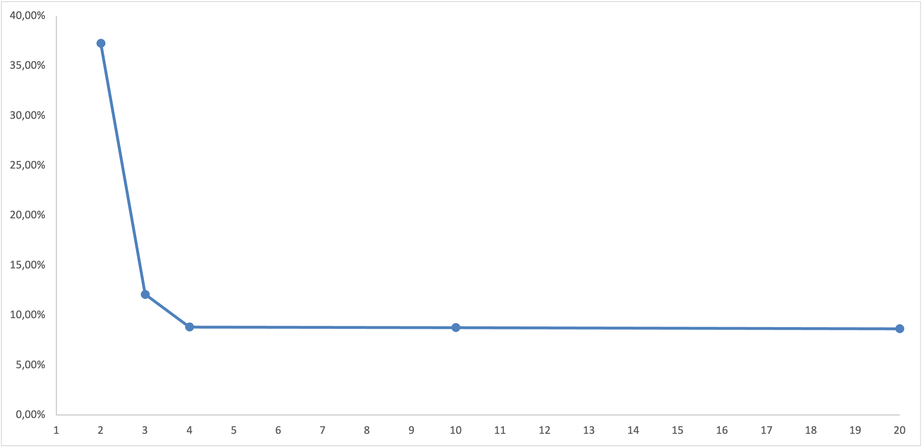
Figure 1: Relative Error of Value function as $N$ grows

Errors are expressed as percentages. Increasing $N$ decreases the relative error. For small $N$, we achieve good results. For example, with $N\geq 4$, the absolute error is less than 10% (round 8%). However, the error does not decrease anymore for $N\geq 4$. This might be explained by the restriction done on the control set.

4.3 A Mean-Variance optimal investment problem

We refer to [16] for a review on portfolio optimization in partial observation framework. We consider a financial market over the horizon $\{0,\ldots,T\}$. We suppose that this market is composed by one asset with return process $(R_{0},\ldots,R_{T})$ satisfying

$$R_{k}=b_{0}\Delta+\sigma\sqrt{\Delta}\epsilon_{k+1}\;,\quad k=0,\ldots,T-1\;,$$

where the drift and the variance $b_{0}$ and $\sigma$ are known. We assume that $(\epsilon_{1},\ldots,\epsilon_{T})$ is a sequence of independent ${\cal N}(0,1)$-distributed random variables independent from $X_{0}$. We consider an investor who can invest at each time on this asset. The wealth process $(X_{0}^{\alpha},\ldots,X_{T}^{\alpha})$ is given by

$$X_{k+1}^{\alpha}=X_{k}^{\alpha}+\alpha_{k}\bigg{(}b_{0}\Delta+\sigma\sqrt{\Delta}\epsilon_{k+1}\bigg{)}\;,\quad k=0,\ldots,T-1\;,$$

Due to a lack of liquidity on this asset, we suppose that the investor does not observe its portfolio directly, but rather an approximate representation $(X_{0}^{\alpha},\ldots,X_{T}^{\alpha})$ is given by

$$Y_{k}^{\alpha}=X_{k}^{\alpha}+\eta_{k}\;,\quad k=1,\ldots,T\;.$$

Such a situation can be faced by private equity investors since they only have some intuition about the value of their portfolios. We refer to [8], [9], [19] for more details. The studied system is then:

$$\left\{\begin{array}[]{ll}X_{k+1}^{\alpha}=X_{k}^{\alpha}+\alpha_{k}\bigg{(}b_{0}\Delta+\sigma\sqrt{\Delta}\epsilon_{k+1}\bigg{)}\;,\\ Y_{k+1}^{\alpha}=X_{k+1}^{\alpha}+\eta_{k+1}\;,~{}~{}~{}~{}~{}~{}k=0,\ldots,T-1\;.\end{array}\right.$$ (4.33)

We suppose that $\eta_{k+1}$ is a sequence of independent ${\cal N}(0,1)$-distributed random variables, also independent from $(\eta_{1},\ldots,\eta_{T})$, $X_{0}$ and $Y_{0}$.

The investor goal is to find a portfolio allocation that minimize a mean-variance criterum:

$$V_{0} = \inf_{\alpha\in\bar{\mathfrak{C}}}J(\alpha)$$

$$= \inf_{\alpha\in\bar{\mathfrak{C}}}\Bigg{[}\frac{\gamma}{2}Var[X_{T}^{\alpha}]-\mathbb{E}[X_{T}^{\alpha}]\Bigg{]}$$

for a $\gamma>0$.

We propose to apply the numerical approximation algorithm of Section 4.2.1. As a starting point, we set the $d=1$, $T=5$. Additionally, we fix $b_{0}=0.02,\sigma=0.05$ for the Return process, so that the investor can expect a return of $0.02$ with a volatility of $0.05$ for this asset. Furthermore, we assume the control space to be $\{0.5,0.75,1,2\}$. Investing only a quarter, half, three quarters, or the entire wealth of an investor is permitted. Using the proposed algorithm with $N=2$, we compute the optimal control at every time $t=0,\ldots,T$. This control leads to a portfolio. Our proposed allocation is benchmarked against two strategies. The first one is known as ’buy and hold’: the investor remains invested in the asset at all times. For the second strategy, it can be viewed as a classical trending strategy: if the asset return is positive at a given time $t$, the investor invests, else the investor shorts the asset. Based on 250 trajectory simulations, we compute the empirical final wealth mean, denoted by $\bar{\mathbb{E}}[X_{T}^{\alpha}]$ and the empirical final wealth variance denoted by $\bar{\text{Var}}[X_{T}^{\alpha}]$. We present in Tables 1, 2, 3 and 4 the results for several values of $\gamma$.

	Proposed Strategy	Buy and Hold	Trending Strategy
$\bar{\mathbb{E}}[X_{T}^{\alpha}]$	1,02027868	1,04535767	1,01155139
$\bar{\text{Var}}[X_{T}^{\alpha}]$	0,00481573	0,00680738	0,00688046
$V_{0}$	-1,01546295	-1,03855029	-1,00467093

Table 1: Empirical Results for $\gamma=2$

	Proposed Strategy	Buy and Hold	Trending Strategy
$\bar{\mathbb{E}}[X_{T}^{\alpha}]$	1,02681514	1,03881421	1,01034027
$\bar{\text{Var}}[X_{T}^{\alpha}]$	0,00467356	0,00653589	0,00636125
$V_{0}$	-1,01746802	-1,02574243	-0,99761777

Table 2: Empirical Results for $\gamma=4$

	Proposed Strategy	Buy and Hold	Trending Strategy
$\bar{\mathbb{E}}[X_{T}^{\alpha}]$	1,02314645	1,03975832	1,00942357
$\bar{\text{Var}}[X_{T}^{\alpha}]$	0,00452504	0,00651461	0,00684134
$V_{0}$	-1,00504629	-1,01369988	-0,98205821

Table 3: Empirical Results for $\gamma=8$

	Proposed Strategy	Buy and Hold	Trending Strategy
$\bar{\mathbb{E}}[X_{T}^{\alpha}]$	1,01748989	1,03562335	1,01643678
$\bar{\text{Var}}[X_{T}^{\alpha}]$	0,00433524	0,00693694	0,006672365
$V_{0}$	-0,98280797	-0,98012783	-0,96305786

Table 4: Empirical Results for $\gamma=16$

With the proposed approach, the variance of the final wealth is systematically smaller for every $\gamma$. The buy-and-hold strategy provides the best returns for investors: however, the proposed strategy reduces variance compared to a buy-and-hold strategy. For example, when $\gamma=2$, the proposed strategy reduces volatility by 41% compared to buy and hold for a return’s cost of 2.45%. We note that the proposed strategy is better in terms of $V_{0}$ value when $\gamma$ is equal to 16. As a result, we have proposed an interesting allocation that can be used to reduce portfolio risk using only two quantization points.

5 Conclusion

A partially observed optimal control problem for a system with mean field discrete time dynamics is presented and solved. We extend the linear-quadratic case (also known as Kalmann Bucy) to deal with the mean field dependence. We also propose a general algorithmic approach based on optimal quantization to approximate the optimal value. We check the robustness of the algorithm empirically with a financial example. Some extensions of the work can be proposed. A first natural question is the estimation of the error of the proposed algorithm. The extension of the results to the continuous time case can also be addressed. This leads to the question of the approximation of the continuous time case by a discrete-time model using an Euler discretization of the continuous problem.

References

• [1] Nasir Uddin Ahmed and Xinhong Ding. Controlled mckean-vlasov equations. Communications on Applied Analysis, 5:183–206, 2001.
• [2] Daniel Andersson and Boualem Djehiche. A maximum principle for sdes of mean-field type. Applied Mathematics and Optimization, 63:341–356, 2010.
• [3] Alain Bensoussan, Jens Frehse, and Phillip Yam. The master equation in mean-field theory. Journal de Math ématiques Pures et Appliqées, 103(6):1441–1474, 2015.
• [4] Rainer Buckdahn, Boualem Djehiche, and Juan Li. A general maximum principle for sdes of mean-field type. Applied Mathematics and Optimization, 64(2):197–216, 2011.
• [5] René Carmona and François Delarue. Forward–backward stochastic differential equations and controlled McKean-Vlasov dynamics. The Annals of Probability, 43(5):2647–2700, 2015.
• [6] Robert Elliott, Xun Li, and Yuan-Hua Ni. Discrete time mean-field stochastic linear-quadric optimal control problems. Automatica, 49(3222-3233), 2013.
• [7] Robert J. Elliott, Lakhdar Aggoun, and John B. Moore. Hidden Markov Models, Estimation and Control, volume 29 of Stochastic Modelling and Applied Probability. Springer Verlag, 1995.
• [8] Paul A Gompers and Josh Lerner. Risk and reward in private equity investments: The challenge of performance assessment. The Journal of Private Equity, pages 5–12, 1997.
• [9] Elise Gourier, Ludovic Phalippou, and Mark M Westerfield. Capital commitment. CEPR Discussion Paper No. DP16910, 2022.
• [10] Julien Guyon and Pierre Henry-Labordere. Nonlinear option pricing. CRC Press, 2013.
• [11] Jianhui Huang, Xun Li, and Jiongmin Yong. A linear-quadratic optimal control problem for mean-field stochastic differential equations in infinite horizon. Mathematical Control and Related Fields, 5(1), 2015.
• [12] Minyi Huang, Roland P. Malhamé, and Peter E. Caines. Large population stochastic dynamic games: closed-loop McKean-Vlasov systems and the nash certainty equivalence principle. Communication in Information and Systems, 6(3):221–252, 2006.
• [13] Jean-Michel Lasry and Pierre-Louis Lions. Mean-field games. Japanese Journal of Mathematics, 2:229–260, 2007.
• [14] Thilo Meyer-Brandis, Bernt Oksendal, and Xun Yu Zhou. A mean field stochastic maximum principle via malliavin calculus. Stochastics An International Journal of Probability and Stochastic Processes, 84(5), 2010.
• [15] Gilles Pagès. Numerical Probability. Springer, 2018.
• [16] Huyên Pham. Portfolio optimization under partial observation: theoretical and numerical aspects. Handbook of Nonlinear Filtering, 2011.
• [17] Huyên Pham and Xiaoli Wei. Discrete time mckean–vlasov control problem: A dynamic programming approach. Applied Mathematics and Optimization, 74(3):487–506, 2016.
• [18] Huyên Pham and Xiaoli Wei. Bellman equation and viscosity solutions for mean-field stochastic control problem. ESAIM: COCV, 24(1):437–461, 2018.
• [19] Tedongap Roméo and Tafolong Ernest. Illiquidity and investment decisions: a survey. Working Paper, 2018.