Simple and accurate screening parameters for dielectric-dependent hybrids

Abstract

A simple effective screening parameter for screened range-separated hybrid is constructed from the compressibility sum rule in the context of linear-response time-dependent Density Functional Theory. When applied to the dielectric-dependent hybrid (DDH), it becomes remarkably accurate for bulk solids compared to those obtained from fitting with the model dielectric function or depending on the valence electron density of materials. The present construction of the screening parameter is simple and realistic. The screening parameter developed in this way is physically appealing and practically useful as it is straightforward to obtain using the average over the unit cell volume of the bulk solid, bypassing high-level calculations of the dielectric function depending on random-phase approximation. Furthermore, we have obtained a very good accuracy for energy band gaps, positions of the occupied $d-$ bands, ionization potentials, optical properties of semiconductors and insulators, and geometries of bulk solids (equilibrium lattice constants and bulk moduli) from the constructed DDH.

I Introduction

Kohn-Sham (KS) density functional theory (DFT) Kohn and Sham (1965); Hohenberg and Kohn (1964) becomes the state-of-the-art method for the electronic structure calculations of solids and materials Burke (2012); Engel and Dreizler (2013); Jones (2015); Cohen et al. (2012); Hasnip et al. (2014); Kümmel and Kronik (2008); Teale et al. (2022). Although it is an exact theory, one must approximate the exchange-correlation (XC) part of KS potential, which includes all the many-body interactions beyond the Hartree theory. The development of new XC approximations having insightful physical content and which are also accurate as well as efficient for solids is always desirable Perdew and Schmidt (2001); Scuseria and Staroverov (2005); Della Sala et al. (2016); Perdew et al. (2008a, 2005). In this respect, semilocal XC approximations Perdew et al. (1996, 2008b); Lee et al. (1988); Perdew et al. (2009); Tao et al. (2003); Tao and Mo (2016); Patra et al. (2019a); Constantin et al. (2016a, b, 2015, 2011); Sun et al. (2015); Furness et al. (2020); Mejía-Rodríguez and Trickey (2020); Jana et al. (2021a, 2019a); Patra et al. (2020); Jana et al. (2021b) are quite useful, because of their efficiency  Singh-Miller and Marzari (2009); Patra et al. (2017); Jana et al. (2018a); Haas et al. (2009); Sun et al. (2011); Tran et al. (2016); Mo et al. (2017); Peng and Perdew (2017); Zhang et al. (2017); Shahi et al. (2018); Jana et al. (2018b); Patra et al. (2021a); Jana et al. (2020a); Ghosh et al. (2021). However, there are limitations when applied these semilocal XC functionals to calculate energy gaps for solids Perdew et al. (2017); Tran et al. (2007); Borlido et al. (2020a); Patra et al. (2019b); Tran et al. (2018); Jana et al. (2018a); Tran and Blaha (2017); Tran et al. (2019), optical spectrum Paier et al. (2008); Wing et al. (2019a); Städele et al. (1999); Petersilka et al. (1996); Kim and Görling (2002); Terentjev et al. (2018); Sharma et al. (2011); Rigamonti et al. (2015); Van Faassen et al. (2002); Cavo et al. (2020); Jana et al. (2020b); Ohad et al. (2022); Wing et al. (2019b); Ramasubramaniam et al. (2019), and semiconductor defects Deák et al. (2019); Lewis et al. (2017); Batista et al. (2006); Deák et al. (2010); Rauch et al. (2021). All these deficiencies of the semilocal XC functionals are related to the known de-localization error Perdew et al. (2017); Shu and Truhlar (2020), which leads to the construction of hybrid functions with fractions of HF mixing Heyd et al. (2003); Krukau et al. (2006); Tao et al. (2008); Heyd and Scuseria (2004); Jana et al. (2020c, b, 2022); Jana and Samal (2018); Patra et al. (2018); Jana et al. (2019b); Jana and Samal (2019); Jana et al. (2018c); Garrick et al. (2020). Although the hybrid XC approximations of DFT solve many problems, they also have some limitations when a fixed HF mixing is used Deák et al. (2019); Wing et al. (2019b); Wang et al. (2016)

Nowadays, hybrid functionals with system-dependent HF mixing are fairly popular methods. Those are known as the dielectric-dependent hybrids (DDHs) Shimazaki and Nakajima (2014); Skone et al. (2014); Brawand et al. (2016); Skone et al. (2016); Chen et al. (2018); Cui et al. (2018); Lorke et al. (2020), where the HF mixing is proportional to the inverse of the macroscopic static dielectric constant of the system under study. Such hybrids are developed and applied to solids for quite some time Gerosa et al. (2015a, b); Miceli et al. (2018); Zheng et al. (2019); Gerosa et al. (2017); Hinuma et al. (2017); Brawand et al. (2017); Liu et al. (2019). DDHs can be considered as the higher rung hybrids than those proposed from regular fixed HF mixing. Also, DDHs are computationally more expensive than regular fixed HF mixed hybrids, in the sense that one needs to calculate the dielectric constant of the material beforehand. However, the great advantages of DDHs are that they are constructed smartly using the same philosophy as COH-SEX (local Coulomb hole plus screened exchange) Grüneis et al. (2014a) by fulfilling many important constraints that the exact XC functional must observe. Therefore, those possess similar accuracy as $GW$ for band gaps and Bethe-Salpeter equation (BSE) for optical spectra Wing et al. (2019a).

Regarding the several recently proposed DDHs, we recall range-separated-DDH (RS- DDH) Brawand et al. (2016); Skone et al. (2016), DDH based on the Coulomb-attenuated method (DD-RSH-CAM) Chen et al. (2018), and doubly-screened DD hybrid (DSH) Cui et al. (2018) based on their range separation. Also, there are other ways of implementing the DDHs such as satisfaction of the Koopmans-theorem Lorke et al. (2020). A fairly good description and comparison of different versions of hybrids are discussed in ref. Liu et al. (2019). Although the system-dependent macroscopic dielectric constant for DDHs is calculated from first principles (such as Perdew-Burke-Ernzerhof (PBE) or random-phase approximation (RPA) on the top of the PBE calculations (RPA@PBE)), the screening parameters are constructed from several philosophies. Such as from the fitting of the long-wavelength limit of highly accurate dielectric functions Chen et al. (2018); Wing et al. (2019a); Liu et al. (2019) calculated from random-phase approximation (RPA) or nanoquanta kernel and partially self-consistent $GW$ calculations Wing et al. (2019a); Liu et al. (2019) or from valance electron density Brawand et al. (2016); Skone et al. (2016); Cui et al. (2018); Lorke et al. (2020). Both are non-empirical choices and required no optimization procedure.

In this work, we propose an alternative procedure for obtaining the range-separated parameter for DDHs using a simple and effective way via the compressibility sum rule, which connects the screening parameter with the exchange energy density. It is quite a realistic way of obtaining the screened parameter, where the relationship can be established through the linear-response time-dependent DFT (TDDFT). Importantly, the present construction gives a very realistic result similar to those obtained from the model dielectric function. We assess the accuracy of screening parameters with DD-RSH-CAM Chen et al. (2018) for the electronic properties of solids, especially energy gaps, geometries, and optical properties.

The rest of the paper is organized as follows. Section II describes the generalized formulation of the range-separated DDH along with the construction of the screening parameter developed in this work. Section III presents results obtained from non-empirical screening parameters using the DD-RSH-CAM for solid properties. Section IV summarizes and concludes the work of this paper.

II Theory

II.1 Generalized form

We start from the Coulomb attenuated method (CAM) style ansatz of the screened-range-separated hybrid (SRSH) functional by partitioning the Coulomb interaction as Kronik and Kümmel (2018),

$$\frac{1}{r}=\frac{\alpha+\beta~{}erf(\mu r)}{r}+\frac{1-[\alpha+\beta~{}erf(\mu r)]}{r}~{},$$ (1)

where $\mu$ is the range-separation parameter. In SRSH, the first term is treated by a Fock-like operator. The second term is treated by semilocal exchange, which is based on the semilocal (SL) GGA functional (PBE) in the present case. However, meta-GGA semilocal functionals can also be used Jana et al. (2022). Following Eq. 1 the expression of the exchange-correlation (XC) functional becomes,

$$\begin{split}E_{xc}^{SRSH}=(1-\alpha)E_{x}^{SR-SL,\mu}+\alpha E_{x}^{SR-HF,\mu}\\ +[1-(\alpha+\beta)]E_{x}^{LR-SL,\mu}+(\alpha+\beta)E_{x}^{LR-HF,\mu}+E_{c}^{SL}~{}.\end{split}$$ (2)

Here, $\alpha$ and $\beta$ control the fraction of short-range and long-range exchange to the above decomposition. $\mu$ is the range-separation parameter. The aforementioned generalized decomposition can take several forms depending on the tuning of $\alpha$ and $\beta$ parameters. For example, (i) with $\beta=-\alpha$, the screened hybrid with SR-HF and LR-SL is recovered. This type of hybrid is useful for solids Heyd et al. (2003); Jana et al. (2020c, b), (ii) with the choice of $\alpha+\beta=1$, in LR, the HF is always recovered Vydrov and Scuseria (2006); Jana et al. (2019b). This type of hybrid is useful for finite systems, especially for the long-range excitation of molecules Kronik et al. (2012), and finally the (iii) the global hybrid functional is obtained by considering $\beta=0$ Ernzerhof and Scuseria (1999).

Though choice (i) is quite convenient for solids and popularly used in the name of Heyd-Scuseria-Ernzerhof (HSE) Heyd et al. (2003), it underestimates the band-gaps of insulators Tran and Blaha (2017) and defect formation energies Deák et al. (2019) because of the lack of dielectric screening. Considering this limitation, the SRSH hybrid has been constructed by proposing the dielectric screening of solids as $\alpha+\beta=\epsilon^{-1}_{\infty}$. This SRSH functional has the following expression

$$\begin{split}E_{xc}^{SRSH}=(1-\alpha)E_{x}^{SR-SL,\mu}+\alpha E_{x}^{SR-HF,\mu}\\ +(1-\epsilon^{-1}_{\infty})E_{x}^{LR-SL,\mu}+\epsilon^{-1}_{\infty}E_{x}^{LR-HF,\mu}+E_{c}^{SL}~{},\end{split}$$ (3)

where $\epsilon^{-1}_{\infty}$ is the inverse of the macroscopic static dielectric constant which is material specific. The main motivation of the underlying approximation is followed from Green’s function based many-body approaches ($GW$ exchange-correlation self-energy methods, $\Sigma_{xc}$), where local Coulomb hole (COH) plus screened exchange (SEX) (COHSEX) are taken into account. (See ref. Cui et al. (2018) for the connection between COHSEX and DDHs.) The corresponding potential of the screened exchange is given as,

$$V_{xc}^{SRSH}({\bf{r,r^{\prime}}}) = [\alpha-(\alpha-\epsilon^{-1}_{\infty})erf(\mu r)]V_{x}^{HF}({\bf{r,r^{\prime}}})$$ (4)

$$- (\alpha-\epsilon^{-1}_{\infty})V_{x}^{SR-SL,\mu}({\bf{r}})+(1-\epsilon^{-1}_{\infty})V_{x}^{SL}({\bf{r}})$$

$$+ V_{c}({\bf{r}})~{},$$

where $V_{x}^{HF}({\bf{r,r^{\prime}}})$ is the full-range HF exchange,

$$V_{x}^{HF}({\bf{r,r^{\prime}}})=-\sum_{n{\bf{k}}}w_{n{\bf{k}}}f_{n{\bf{k}}}\frac{\phi^{KS}_{n{\bf{k}}({\bf{r^{\prime}}})}\phi^{KS}_{n{\bf{k}}}({\bf{r}})}{|{\bf{r}}-{\bf{r}^{\prime}}|}~{},$$ (5)

$\phi^{KS}_{n{\bf{k}}}$’s are the KS orbitals or basis, $V_{x}^{SL}({\bf{r}})$ is the full-range semilocal functional, which is PBE functional in the present case, $V_{x}^{SR-SL,\mu}({\bf{r}})$ is the short-range (SR) part of the PBE functional, and $V_{c}({\bf{r}})$ is the PBE correlation. It may be noted that for solids the reciprocal space representation of $erf(\mu r)$ becomes $e^{-|\bf{G}|^{2}/(4\mu)}$, where $\bf{G}$ is the reciprocal lattice vector. Several choices of the $\alpha$, $\epsilon^{-1}$, and $\mu$ exist and based on those choices rungs of screened exchange or DDHs functionals may be constructed (see ref. Liu et al. (2019) for details).

In particular, we consider the case $\alpha=1$ which is used in the doubly screened hybrid (DSH) of Ref. Cui et al. (2018) and in the dielectric-dependent range-separated hybrid functional based on the Coulomb-attenuating method (CAM) (DD-RSH-CAM) Chen et al. (2018). In the later case, the model dielectric function is

$$\varepsilon^{-1}({\bf{G}})=1-(1-\epsilon^{-1}_{\infty})e^{-|\bf{G}|{{}^{2}}/(4\mu)}.$$ (6)

However, the accuracy of Eq. 3 depends on two main aspects:

(i) The macroscopic static dielectric constant, $\epsilon^{M}_{\infty}$: is mostly calculated in a first-principles way using the linear response TDDFT method Souza et al. (2002); Nunes and Gonze (2001); Gajdoš et al. (2006). The RPA@PBE dielectric constants are reasonably well described Chen et al. (2018). For hybrids or DDHs, the dielectric constants are calculated using RPA+$f_{xc}$, where $f_{xc}$ is the XC kernel Chen et al. (2018); Liu et al. (2019). Although there are several XC kernels (see ref. Olsen et al. (2019) for a review), we recall that for DD-RSH-CAM, the bootstrap approximation of Sharma et. al. Sharma et al. (2011) ($f_{xc}^{bootstrap}$) is used.

(ii) The screening parameter, $\mu$: is obtained following several procedures such as: (a) from the fitting of the model dielectric function (Eq. 6) with the long-wavelength limit of the diagonal elements of dielectric function i.e., $\varepsilon^{-1}_{{\bf{G,G}}}({\bf{q}}\to 0,\omega=0)$ obtained from RPA calculations as mentioned in ref. Chen et al. (2018). However, to obtain an accurate dielectric function, one needs additional calculations of highly accurate RPA (and/or “nanoquanta” kernel combined with partially self-consistent $GW$) Chen et al. (2018). (b) Alternatively, the screening parameter, $\mu$ can also be obtained from the valence electron density of the system as referred in Refs. Brawand et al. (2016); Skone et al. (2016); Cui et al. (2018).

In the following, we propose a simple expression for the screening parameter $\mu$, derived from the linear response TDDFT approach.

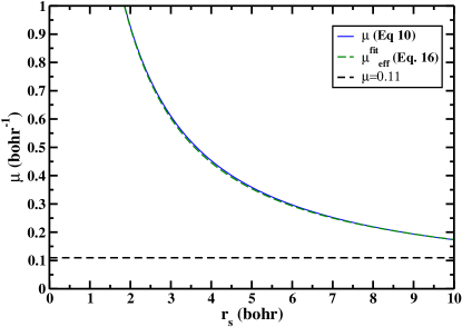
Figure 1: Shown is the $\mu(r_{s})$ as a function of local Seitz radius, $r_{s}$ for $0<r_{s}<10$ bohr.

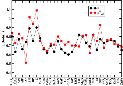
Figure 2: Comparison of $\mu$ values for several solids.

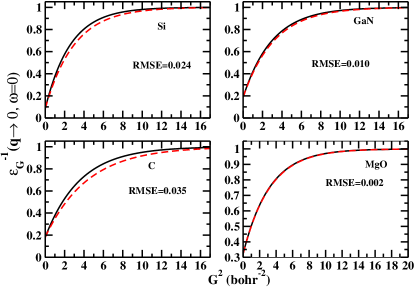
Figure 3: Comparison of model dielectric function as a function of ${\bf{G}}$ for four solids. Black solid line for the $\mu$ values of ref. Chen et al. (2018), whereas red dotted line for $\mu_{eff}^{fit}$. Relative mean square error (RMSE) of the model dielectric function as obtained from $\mu_{eff}^{fit}$ from the actual one (obtained using $\mu$) is also shown.

II.2 Construction of the screening parameter

In the linear-response TDDFT, the interacting ($\chi(\mathbf{r},\mathbf{r}^{\prime};\omega)$) and noninteracting ($\chi_{0}(\mathbf{r},\mathbf{r}^{\prime};\omega)$) density-density response functions are connected by the following Dyson like equation Gross et al. (1996),

$$\chi({\bf{r}},{\bf{r^{\prime}}};\omega)=\chi_{0}({\bf{r}},{\bf{r^{\prime}}};\omega) + \int d{\bf{r}}_{1}d{\bf{r}}_{2}~{}\chi_{0}({\bf{r}},{\bf{r^{\prime}}};\omega)$$ (7)

$$\times v_{eff}[n]({\bf{r}},{\bf{r^{\prime}}};\omega)\chi({\bf{r}},{\bf{r^{\prime}}};\omega)~{},$$

where

$$v_{eff}[n]({\bf{r}},{\bf{r^{\prime}}};\omega)=\frac{1}{|{\bf{r}}-{\bf{r}}^{\prime}|}+f_{xc}[n]({\bf{r}},{\bf{r^{\prime}}};\omega)$$ (8)

is Coulomb plus XC kernel known as the effective potential. If $f_{xc}[n]({\bf{r}},{\bf{r^{\prime}}};\omega)$ is zero, then the RPA Harris and Griffin (1975); Langreth and Perdew (1977) is recovered. Therefore, $f_{xc}[n]({\bf{r}},{\bf{r^{\prime}}};\omega)$ should account for the short-range correlation, which is missing in RPA. Following these considerations, Constantin and Pitarke (CP) proposed a simple and accurate approximation of $v_{eff}[n]({\bf{r}},{\bf{r^{\prime}}};\omega)$ for the three-dimensional (3D) uniform electron gas (UEG) Constantin and Pitarke (2007); Constantin (2016)

$$v^{CP}_{eff}[n]({\bf{r}},{\bf{r^{\prime}}};\omega)=\frac{{\rm erf}(|{\bf{r}}-{\bf{r}}^{\prime}|/\sqrt{4k_{n,\omega}})}{|{\bf{r}}-{\bf{r}}|}.$$ (9)

Note that we already consider this type of splitting in the Coulomb interaction of DDH construction. Also, $4k_{n,\omega}$ is a frequency and density-dependent function that controls the long-range effects of bare Coulomb interaction. Therefore, a direct connection between $4k_{n,\omega}$ and screened parameter $\mu$ can be established as follows,

$$\mu=\mu_{eff} = \frac{1}{\sqrt{4k_{n,\omega=0}}}~{}.$$ (10)

Here, we denote $\mu_{eff}$ as the “effective” screening to distinguish it from the actual screening parameter used in the DD-RSH-CAM. Note that for the DDH functionals of the ground-state DFT, we have to consider the static ($\omega=0$) case.

The XC kernel for 3D UEG can be derived using the Fourier transform of Eqs. 8 and  9 as Constantin and Pitarke (2007)

$$f_{xc}(n;q,\omega)=\frac{4\pi}{q^{2}}[e^{-k_{n,\omega}q^{2}}-1]~{}.$$ (11)

Thus in the long-wavelength ($q\to 0$) limit, one can obtain,

$$k_{n,\omega}=-\frac{1}{4\pi}f_{xc}(n;q\to 0,\omega)~{}.$$ (12)

On the other hand, the long-wavelength limit of the static XC kernel $f_{xc}(n;q\to 0,\omega=0)$ satisfies the compressibility sum rule Ichimaru (1982),

$$f_{xc}(n;q\to 0,\omega=0)=\frac{d^{2}}{dn^{2}}(n\epsilon_{xc}(n))$$ (13)

where $\epsilon_{xc}(n)$ is the XC energy per particle of the 3D UEG. We use the Perdew and Wang parametrization of the local density approximation (LDA) correlation energy per particle Perdew and Wang (1992). Note that the LDA XC kernel is remarkably accurate for $q<2q_{F}$ ($q_{F}=(3\pi^{2}n)^{1/3}$ being the Fermi wavevector), which explains the success of LDA (and semilocal functionals that recover LDA for the 3D UEG) for bulk solids Perdew et al. (1977); Moroni et al. (1995).

Finally, Eqs. 12 and  13 give

$$k_{n,\omega=0}=-\frac{1}{4\pi}\frac{d^{2}}{dn^{2}}[n\epsilon_{xc}(n)]~{},$$ (14)

and $\mu_{eff}$ can be found from Eq. 10. Noteworthy, Eq. 10 is the central equation of this paper, which establishes a direct connection between the screening parameter and the LDA XC energy per particle ( $\epsilon_{xc}(n)$ )Perdew and Wang (1992) which depends only on the local Seitz radius, $r_{s}=(\frac{3}{4\pi n})^{1/3}$ and the relative spin polarization, $\zeta=\frac{n_{\uparrow}-n_{\downarrow}}{n}$.

To simplify the computational implementation for bulk solids, we consider the average of $r_{s}$ over the unit cell volume, $\Omega_{cell}$ as,

$$\langle r_{s}\rangle=\frac{1}{\Omega_{cell}}\int_{cell}\Big{(}\frac{3}{4\pi(n_{\uparrow}({\bf{r^{\prime}}})+n_{\downarrow}({\bf{r^{\prime}}}))}\Big{)}^{1/3}~{}d^{3}r^{\prime}~{}.$$ (15)

We recall that this averaging technique over the unit cell has been considered earlier, e.g. in the construction of the modified Becke-Johnson (MBJ) semilocal exchange potential  Tran and Blaha (2009); Borlido et al. (2020b); Rauch et al. (2020a, b); Tran et al. (2021); Patra et al. (2021b), local range separated hybrid functionals Marques et al. (2011), and XC kernel for optical properties of semiconductors  Terentjev et al. (2018). Thus, for computational simplicity, we fit the exact $\mu_{eff}(r_{s})$ curve with the following formula,

$$\mu_{eff}^{fit}=\frac{a_{1}}{\langle r_{s}\rangle}+\frac{a_{2}\langle r_{s}\rangle}{1+a_{3}\langle r_{s}\rangle^{2}}~{},$$ (16)

where $a_{1}=1.91718$, $a_{2}=-0.02817$, and $a_{3}=0.14954$.

In Fig. 1, we plot $\mu(r_{s})$ versus $r_{s}$ for $0<r_{s}<10$ bohr. As one can see, $\mu_{eff}(r_{s})$ and $\mu_{eff}^{fit}$ agree very well, the curves being almost indistinguishable. We also observe that $\mu_{eff}$ is significantly bigger than the HSE one ($\mu^{HSE}=0.11$), and only in the low-density regime ($r_{s}>10$) they become comparable. As a side note, $\mu_{eff}(r_{s})$ seems also very realistic for LC-type hybrid functionals, where $\mu^{LC}\approx 0.50$ bohr^-1, (see for example Table IV of Ref. Jana et al. (2019b)), because $\mu_{eff}(r_{s})>0.5$ bohr^-1 for $r_{s}<3.6$ bohr and $\mu_{eff}(r_{s})<0.50$ bohr^-1 for $r_{s}>3.6$ bohr.

III Results

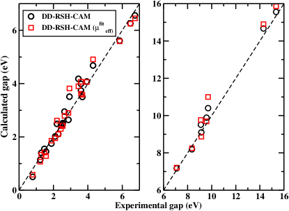
Figure 4: Shown is the calculated versus experimental band gaps of $32$ solids using different methods. $\epsilon_{\infty}^{-1}$ obtained from DD-RSH-CAM is considered here.

Table 1: Screening parameters, $\mu$ (in bohr ^-1) and band gap energies, $E_{g}$ (in eV) of the $32$ semiconductors and insulators calculated using different dielectric constants. Band gaps are corrected for spin-orbit coupling as mentioned in ref. Chen et al. (2018). MAE of screening parameters (with respect to DD-RSH-CAM) and band gaps (with respect to Expt.+ZPR) are in bohr ^-1 and eV, respectively.

	$\mu$ (bohr-1)		Eg (eV)
Solids	Ref. Chen et al. (2018)	$\mu_{eff}^{fit}$		Cal.a	Cal.b	Expt.+ZPR Chen et al. (2018)
Al2O3	0.80	0.84		9.76	9.87	9.10
AlAs	0.63	0.73		2.10	2.17	2.28
AlN	0.77	0.83		6.25	6.23	6.47
AlP	0.66	0.78		2.43	2.39	2.54
Ar	0.74	0.51		14.90	15.19	14.30
BN	0.89	1.02		6.45	6.49	6.74
BP	0.75	0.94		1.95	1.91	2.10
C	0.90	1.09		5.59	5.59	5.85
CaO	0.78	0.75		7.21	7.07	7.09
CdS	0.66	0.67		2.79	2.65	2.64
CdSe	0.62	0.64		1.86	1.84	1.88
Cu2O	0.70	0.72		2.61	2.24	2.20
GaAs	0.63	0.71		1.28	1.34	1.57
GaN	0.75	0.80		3.58	3.51	3.68
GaP	0.66	0.75		2.30	2.26	2.43
Ge	0.62	0.71		0.58	0.62	0.79
In2O3	0.60	0.74		3.82	3.65	2.93
InP	0.63	0.70		1.41	1.35	1.47
LiCl	0.70	0.70		9.69	9.69	9.57
LiF	0.82	0.69		15.86	16.35	15.35
MgO	0.80	0.81		8.25	8.31	8.36
MoS2	0.73	0.82		1.33	1.30	1.29
NaCl	0.69	0.62		8.87	8.90	9.14
NiO	0.82	0.82		4.91	4.21	4.30
Si	0.65	0.75		1.07	1.04	1.23
SiC	0.77	0.93		2.41	2.39	2.53
SiO2	0.73	0.67		11.00	11.16	9.70
SnO2	0.75	0.76		3.62	3.62	3.60
TiO2	0.76	0.77		3.90	3.57	3.45
ZnO	0.75	0.72		4.07	3.66	3.60
ZnS	0.69	0.71		4.06	3.94	3.94
ZnSe	0.65	0.68		2.90	2.92	2.87
MAE		0.07c		0.29d	0.25d

a) calculated using $\epsilon_{\infty}^{-1}$ obtained from DD-RSH-CAM and $\mu_{eff}^{fit}$.

b) calculated using $\epsilon_{\infty}^{-1}$ obtained from RPA@PBE and $\mu_{eff}^{fit}$.

c) MAE in bohr^-1 with respect to the $\mu$ calculated in Ref. Chen et al. (2018) for DD-RSH-CAM.

d) MAE in eV with respect to experimental.

Table 2: Mean positions of the occupied $d$ band (in eV) relative to the VBM for selective semiconductors. The theoretical values are calculated by averaging the $d$ state energies at the $\Gamma$ point.

Solids		Calculateda		Calculatedb	$GW\Gamma^{1}$@HSE06d	Expt.c
CdS		9.9		10.0	9.5	9.6
CdSe		10.3		10.2	9.7	10
InP		17.1		17.1	16.9	16.8
GaAs		20.3		20.3	18.5	18.9
GaN		18.1		18.1	17.0	17.0
GaP		19.8		19.8	18.3	18.7
ZnO		7.3		7.9	7.1	7.5
ZnS		9.5		9.8	8.4	9.0
ZnSe		10.1		10.2	8.6	9.2
MAE		0.7		0.7	0.3

a) calculated using $\epsilon_{\infty}^{-1}$ obtained from DD-RSH-CAM and $\mu_{eff}^{fit}$.

b) calculated using $\epsilon_{\infty}^{-1}$ obtained from RPA@PBE and $\mu_{eff}^{fit}$.

c) See Table VI of ref. Chen et al. (2018) for experimental values.

d) From ref. Grüneis et al. (2014a).

Table 3: Ionization potentials (IPs) and electron affinities (EAs) (where EA=IP-E_g in eV) of II-VI and III-V semiconductors as obtained from different methods.

	PBE		HSE06 Grüneis et al. (2014a)		DD-RSH-CAM    ($\mu_{eff}^{fit}$)a		$GW\Gamma^{1}$@HSE06 Grüneis et al. (2014a)		Expt. Grüneis et al. (2014a)
Solids	IP	EA	IP	EA	IP	EA	IP	EA	IP	EA
AlAs	5.25	3.86	5.19	3.09	5.52	3.42	5.97	3.52	5.66	3.50
AlP	5.71	4.11	5.65	3.36	6.03	3.60	6.40	3.68	6.43	3.98
CdS	5.97	4.96	6.56	4.37	6.55	3.76	6.94	4.35	6.10	3.68
CdSe	5.60	5.24	6.06	4.48	5.99	4.12	6.62	4.71	6.62	4.50
GaAs	4.87	4.28	5.16	3.73	4.82	3.54	5.38	3.85	5.59	4.07
GaP	5.50	3.97	5.74	3.43	5.63	3.33	5.85	3.32	5.91	3.65
Ge	4.69	4.62	4.60	3.78	4.33	3.75	4.98	4.15	4.74	4.00
InP	5.15	4.74	5.60	4.10	5.10	3.69	5.74	4.16	5.77	4.35
Si	4.89	4.30	5.21	4.04	4.97	3.90	5.46	4.11	5.22	4.05
ZnS	6.09	4.11	6.74	3.42	7.13	3.06	7.18	3.29	7.50	3.90
ZnSe	5.61	4.61	6.15	3.71	6.44	3.54	6.71	3.79	6.79	4.09
MAE (eV)	0.63	0.51	0.42	0.33	0.43	0.38	0.21	0.28
MAPE	9.96	12.92	6.60	8.54	7.18	9.43	3.64	7.07

a) Calculated using $\epsilon_{\infty}^{-1}$ obtained from DD-RSH-CAM and $\mu_{eff}^{fit}$.

Table 4: Lattice constant (a₀) and bulk modulus (B₀) for selective solids. MAEs of lattice constants and bulk moduli are in Å and GPa, respectively.

	a0 (Å)			B0 (GPa)
Solids	Calculateda	Calculatedb	Expt.	Calculateda	Calculatedb	Expt.
AlP	5.477	5.478	5.445c	86.8	86.5	87.4d
AlAs	5.677	5.678	5.646c	73.1	72.9	75.0d
BN	3.592	3.591	3.585c	399.7	416.4	410.2d
BP	4.531	4.532	4.520c	165.0	168.3	168.0d
CdS	5.908	5.911	5.808c	58.8	58.4	64.3d
CdSe	6.163	6.169	6.042c	49.4	48.9	55.0d
C	3.551	3.551	3.544c	454.8	454.8	454.7d
CaO	4.770	4.771	4.787c	121.2	120.8	110.0c
GaP	5.458	5.460	5.435c	87.0	86.6	89.6e
GaAs	5.657	5.660	5.637c	71.5	71.0	76.7e
Ge	5.679	5.684	5.639c	68.4	67.6	77.3e
InP	5.928	5.939	5.856c	70.5	67.1	72.0e
LiCl	5.068	5.067	5.072c	35.0	35.0	38.7e
LiF	3.920	3.916	3.960c	86.1	86.7	76.3e
MgO	4.148	4.148	4.186c	182.8	183.1	169.8e
NaCl	5.554	5.553	5.565c	27.3	27.3	27.6e
SiC	4.352	4.352	4.340c	229.7	229.7	229.1e
Si	5.444	5.449	5.415c	95.0	91.0	100.8e
ZnS	5.455	5.457	5.399c	72.0	71.5	77.2d
ZnSe	5.682	5.685	5.658c	63.4	63.4	64.7d
MAE	0.035	0.037		4.8	4.8
MAPE	0.652	0.693		5.3	5.3

a) Calculated using $\epsilon_{\infty}^{-1}$ obtained from DD-RSH-CAM and $\mu_{eff}^{fit}$.

b) Calculated using $\epsilon_{\infty}^{-1}$ obtained from RPA@PBE and $\mu_{eff}^{fit}$.

c) Taken from Ref. Haas et al. (2009), where the experimental lattice constants were corrected for zero-point anharmonic expansion (ZPAE).

d) ZPAE corrected bulk moduli values from Ref. Zhang et al. (2018). e) ZPAE corrected bulk moduli values from Ref. Schimka et al. (2011).

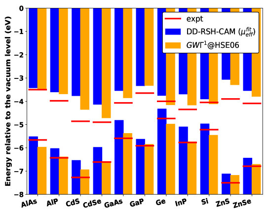
Figure 5: Band alignment of for II-VI and III-V semiconductors based on the IPs (negatives of the VBM to the vacuum level) and EAs (negatives of CBM to the vacuum level) as obtained from DD-RSH-CAM ($\mu_{eff}^{fit}$). For comparison, $GW\Gamma^{1}$@HSE06 Grüneis et al. (2014a) (shown by the bar) and experimental values (shown by a straight line) are also shown. All the surface orientations are along (110) directions.

We combine $\mu_{eff}^{fit}$ with DD-RSH-CAM to obtain the properties of solids. Unless otherwise stated DD-RSH-CAM denoted in this work is the original DDH presented in ref. Chen et al. (2018), whereas DD-RSH-CAM($\mu_{eff}^{fit}$) corresponds to the present work.

In Fig. 2, we compare $\mu$ and $\mu_{eff}^{fit}$ values for several solids, obtained from fitting with the model dielectric function and using the method described in this paper, respectively. We observe a fairly good agreement, except for a few solids like BN, C, SiC, and Ar. For the BN, C, and SiC bulk solids, $\mu_{eff}^{fit}$ overestimates over $\mu$ with less or about $\sim 0.19$ bohr^-1, while for the Ar solid, $\mu_{eff}^{fit}$ underestimates over $\mu$ with about $0.25$ bohr^-1. One may note that larger $\mu$ values correspond to more HF mixing.

Fig. 3 compares the model dielectric function as a function of reciprocal lattice vector, ${\bf{G}}$. As observed from the relative mean square error (RMSE), a maximum deviation of $0.035$ is obtained for C, whereas we observe a very good agreement for MgO. The overall analysis of Figs. 1 and  3 suggests that the constructed $\mu_{eff}^{fit}$ from the compressibility sum rule is as good as $\mu$ obtained from the least-squares fit of the model dielectric function.

III.1 Energy gap and valence band structure

Table 1 compiles the energy gaps of $32$ semiconductors and insulators using the static dielectric constants obtained either from RPA@PBE or DD-RSH-CAM method. We consider a similar test set as the one of ref. Chen et al. (2018) for DD-RSH-CAM. One may note that the static dielectric constants that are obtained from DD-RSH-CAM are quite realistic Chen et al. (2018) (see Table TABLE IV of ref. Chen et al. (2018)). In Table 1 we also show a good agreement between $\mu_{eff}^{fit}$ and $\mu$ for all the considered bulk solids, and the mean absolute deviation of $\mu_{eff}^{fit}$ is $0.07$ bohr^-1 compared to $\mu$.

Next, we compare energy gaps for different solids and we observe a fairly good agreement when calculations are performed using $\varepsilon_{\infty}^{-1}$ of DD-RSH-CAM and $\mu_{eff}^{fit}$. One may note that in ref. Chen et al. (2018), $\varepsilon_{\infty}^{-1}$ are obtained using the $f_{xc}^{bootstrap}$ kernel Sharma et al. (2011). However, when calculations are performed with $\varepsilon_{\infty}^{-1}$ from the RPA@PBE method, with $\mu_{eff}^{fit}$, a slight overestimation in band gaps of insulating solids are observed (such as for Ar and LiF). This originated because for those solids RPA@PBE underestimates $\varepsilon_{\infty}^{-1}$, compared to DD-RSH-CAM. However, both panels of results for band gaps of Table 1 give an overall mean absolute error (MAE) $\sim$0.3 eV with respect to the experimental, indicating very good agreement with that of the DD-RSH-CAM Chen et al. (2018).

Finally, Fig. 4 compares the experimental versus calculated band gaps for DD-RSH-CAM and DD-RSH-CAM ($\mu_{eff}^{fit}$). We observe that both methods match quite well, except few large gap solids, where slight overestimation in band gaps is observed from DD-RSH-CAM ($\mu_{eff}^{fit}$). Furthermore, band gap predictions are not very sensitive to the choice of screening parameter, $\mu$. Overall, we observe all calculated band gaps are close to that of DD-RSH-CAM Chen et al. (2018).

Next, we calculate the mean positions of the occupied $d$ band of selective semiconductors and the results are reported in Table 2. It is well known that approximate DFT XC functionals suffer from de-localization errors. Hence the average position of the occupied $d$ state is underestimated, even for hybrids with fixed HF percentage. As shown in ref. Chen et al. (2018), DD-RSH-CAM can recover positions of the occupied $d$ band correctly. A very similar performance is also observed from Table 2 for DD-RSH-CAM ($\mu_{eff}^{fit}$), which owns MAE of $\sim 0.7$ eV (for both cases of computing $\varepsilon_{\infty}^{-1}$). These results are significantly close to that of higher-level methods such as $GW\Gamma^{1}$@HSE06 Grüneis et al. (2014a).

III.2 IPs and EAs

Another serious assessment of the DDHs is to the determination of absolute band positions, hence ionization potentials (IPs) and electron affinities (EAs) calculated using the slab model Jiang and Shen (2013); Jiang and Blaha (2016); Grüneis et al. (2014b); Hinuma et al. (2014); Ghosh et al. (2022). As stated previously, due to the self-interaction error (SIE) (or delocalization error), semilocal functionals tend to underestimate relative band positions. Therefore, it is interesting to assess the performance of DD-RSH-CAM for extended systems, where the magnitude of SIE strongly depends on the screening nature of the material under consideration. Here, we report IPs and EAs for II-VI and III-V semiconductors using DD-RSH-CAM ($\mu_{eff}^{fit}$). We do not include DD-RSH-CAM as we expect very similar performance.

Since a direct implementation of the DDHs to the slab model is not feasible because of the high computational cost, a more trivial way of doing this is to incorporate the corrections to the VBM state of the bulk system from DDHs. Whereas, the surface supercell slab calculations are performed using semilocal LDA/GGA approximations. In the present case, we use Perdew-Burke-Ernzerhof (PBE) GGA functional. We recall, this method is similar to that of the quasi-particle (QP) $GW$-VBM approach as proposed in ref. Jiang and Shen (2013); Jiang and Blaha (2016). Following the protocols of $GW$-VBM method Jiang and Shen (2013); Jiang and Blaha (2016), the ionization potential at the DDHs level theory can also be defined as

$$\rm IP^{DDH}=IP^{SL}-\Delta\varepsilon_{VBM}^{DDH}~{}.$$ (17)

Here, $\rm IP^{SL}$ is the IPs calculated in the semilocal level (LDA/GGA) as follows,

$$\rm IP^{SL}=[\epsilon_{\mathrm{Vac,s}}-\epsilon_{\mathrm{Ref,s}}]-[\epsilon_{\mathrm{VBM,b}}-\epsilon_{\mathrm{Ref,b}}]~{},$$ (18)

and the corrections or shift to the VBM of the bulk solid because of DDH ($\Delta\varepsilon_{VBM}^{DDH}$) is given by,

$$\rm\Delta\varepsilon_{VBM}^{DDH}=[\epsilon_{\mathrm{VBM,b}}^{DDH}-\epsilon_{\mathrm{Ref,b}}^{DDH}]-[\epsilon_{\mathrm{VBM,b}}-\epsilon_{\mathrm{Ref,b}}]~{}.$$ (19)

Here, $\epsilon_{\mathrm{Vac,s}}-\epsilon_{\mathrm{Ref,s}}$ is calculated for the surface supercell from semilocal functionals, which is PBE for the present case. For both the zincblende ($zb$) and diamond structures, we construct the surface supercell along the (110) direction. $\rm\epsilon_{\mathrm{Vac,s}}$ and $\rm\epsilon_{\mathrm{Ref,s}}$ are the macroscopic average of the local electrostatic potential in the vacuum and the bulk region of the supercell, respectively. From bulk calculations of semilocal and DDHs, $\rm\epsilon_{\mathrm{VBM,b}}-\epsilon_{\mathrm{Ref,b}}$ and $\epsilon_{\mathrm{VBM,b}}^{DDH}-\epsilon_{\mathrm{Ref,b}}^{DDH}$ are determined, with $\epsilon_{\mathrm{VBM,b}}$ (or $\epsilon_{\mathrm{VBM,b}}^{DDH}$) being the position of VBM in semilocal (or DDH) and $\epsilon_{\mathrm{Ref,b}}$ ($\epsilon_{\mathrm{Ref,b}}^{DDH}$) is the reference level for the bulk calculation for semilocal (or DDH), i.e., the average of the electrostatic potential in the unit cell. We show IPs and EAs of DD-RSH-CAM ($\mu_{eff}^{fit}$) along with the HSE06 and $GW\Gamma^{1}$@HSE06 in Table 3. The VBM position (calculated from IPs and EAs) from DD-RSH-CAM ($\mu_{eff}^{fit}$) are also shown in Fig. 5 along with experimental IPs and EAs. As shown in Table 3 and Fig. 5, we observe that for II-VI and III-V semiconductors, IPs and EAs as obtained from DD-RSH-CAM ($\mu_{eff}^{fit}$) are well respected and have similar accuracy with the HSE06 ones. One may note that for II-VI and III-V solids, the performance of HSE06 is respectable Grüneis et al. (2014b), as those are medium-range band gap solids and HSE06 describes well their screening. The similar accuracy of DD-RSH-CAM ($\mu_{eff}^{fit}$) indicates that DD-RSH-CAM ($\mu_{eff}^{fit}$) functional might also be a good choice for electronic structure calculations of semiconductors defects Lorke et al. (2020); Stein et al. (2010); Nguyen et al. (2018); Deák et al. (2019), where HSE06 with fixed mixing parameter is not sufficient Deák et al. (2019).

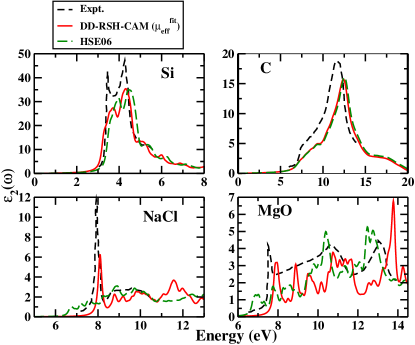
Figure 6: The absorption spectra of Si, C, NaCl, and MgO, calculated with DD-RSH-CAM ($\mu_{eff}^{fit}$) and HSE06. Experimental spectra are taken from Ref. BIRKEN et al. (1998) (for Si), Ref. Logothetidis et al. (1986) (for C), Ref. Roessler and Walker (1968) (for NaCl), Ref. Bortz et al. (1990) (for MgO). Calculations of DD-RSH-CAM ($\mu_{eff}^{fit}$) are performed with DD-RSH-CAM’s $\epsilon_{\infty}^{-1}$.

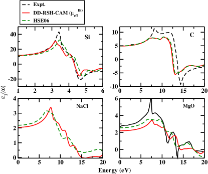
Figure 7: $\epsilon_{1}(\omega)$ for Si, C, and MgO calculated with DD-RSH-CAM ($\mu_{eff}^{fit}$) and HSE06. The Si and C experimental data are taken from Ref. Kootstra et al. (2000), and the MgO experimental data is from ref. Roessler and Walker (1967). Calculations of DD-RSH-CAM ($\mu_{eff}^{fit}$) are performed with DD-RSH-CAM’s $\epsilon_{\infty}^{-1}$.

III.3 Optical absorption spectra

Hybrids functionals include non-local potential, which is the key for improving optical properties of bulk solids Ullrich (2011); Paier et al. (2008); Yang et al. (2015); Wing et al. (2019a); Städele et al. (1999); Petersilka et al. (1996); Kim and Görling (2002); Sun and Ullrich (2020); Sun et al. (2020); Kootstra et al. (2000). The optical absorption spectra as obtained from DDHs are realistic Tal et al. (2020), including excitonic effects i.e., $\sim\frac{1}{\epsilon_{\infty}^{-1}q^{2}}$ in the long-wavelength limit ($q\to 0$)Paier et al. (2008); Wing et al. (2019a). The performance of DD-RSH-CAM is studied in ref. Tal et al. (2020). Therefore, those spectra are not shown in this work. We also recall that several low-cost XC kernels are available to compute optical properties of semiconductors and insulators Trevisanutto et al. (2013); Terentjev et al. (2018); Sharma et al. (2011); Rigamonti et al. (2015); Van Faassen et al. (2002); Cavo et al. (2020); Byun and Ullrich (2017); Byun et al. (2020), describing well the excitons and excitonic effects (e.g. Bootstrap Sharma et al. (2011) and JGM  Trevisanutto et al. (2013); Terentjev et al. (2018) kernels), in contrast to the RPA and adiabatic LDA (ALDA) kernels.

All calculations of DD-RSH-CAM ($\mu_{eff}^{fit}$) are performed by solving the Casida equation as mentioned in ref. Tal et al. (2020). To assess the performance of the DD-RSH-CAM ($\mu_{eff}^{fit}$), we calculate the imaginary ($\epsilon_{2}(\omega)$) and real ($\epsilon_{1}(\omega)$) parts of the macroscopic dielectric function $\epsilon^{M}$ of Si, C, MgO, and NaCl in the optical limit of small wave vectors,

$$\epsilon_{2}(\omega) = \Im\{\lim_{q\rightarrow 0}\epsilon^{M}(q,\omega)\}$$

$$\epsilon_{1}(\omega) = \Re\{\lim_{q\rightarrow 0}\epsilon^{M}(q,\omega)\}.$$ (20)

We recall that the optical absorption spectrum is given by $\epsilon_{2}(\omega)$, while other optical properties (e.g. Fresnel reflectivity at normal incidence, and the long-wavelength limit of the electron-energy-loss function) depend on both $\epsilon_{1}(\omega)$ and $\epsilon_{2}(\omega)$.

The optical spectra are shown in Fig. 6. For the Si bulk, we observe quite realistic absorption spectra from DD-RSH-CAM ($\mu_{eff}^{fit}$), showing two excitation peaks at the right positions corresponding to the experimental. However, the first peak at $\sim 3.5$ eV, which represents the oscillator strength is always underestimated, similar to the hybrids with fixed mixing parameters. A similar performance is also observed for DD-RSH-CAM as shown in ref. Tal et al. (2020). Next, considering the optical spectra of the medium gap semiconductor C diamond, the DD-RSH-CAM ($\mu_{eff}^{fit}$) peak is blueshifted with about $1$ eV, because of the slightly larger value of $\mu_{eff}^{fit}$ (see Fig. 2). However, we obtain reasonable absorption spectra of NaCl and MgO insulators, that is considered difficult tests for all the computational methods. Compared to the absorption spectra of DD-RSH-CAM, as studied in ref. Tal et al. (2020), we see similar tendencies from the present method. One may also note from Fig. 6, that for the wide band gap insulators, the performance of HSE06 is unsatisfactory, underestimating the absorption peak.

Furthermore, in Fig. 7, we show the real part of the dielectric function. In the cases of Si and C, both the TDDFT spectra of DD-RSH-CAM ($\mu_{eff}^{fit}$) and HSE06 are in excellent agreement with the experimental data. However, for the NaCl and MgO insulators, DD-RSH-CAM ($\mu_{eff}^{fit}$) is more realistic, and the peaks are in the correct positions.

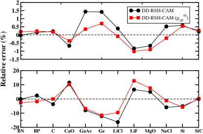
Figure 8: DD-RSH-CAM and DD-RSH-CAM ($\mu_{eff}^{fit}$) relative errors (in %) for the equilibrium lattice constants (upper panel) and bulk moduli (lower panel) of several bulk solids. The DD-RSH-CAM results are from ref. Chen et al. (2018). The calculated mean absolute percentage errors (MAPEs) of DD-RSH-CAM and DD-RSH-CAM ($\mu_{eff}^{fit}$) for lattice constants are obtained to be 0.6% and 0.4%, respectively. For bulk moduli, MAPEs are 6% for both cases.

III.4 Structural properties

Next, we have calculated the structural properties of selective solids with DD-RSH-CAM ($\mu_{eff}^{fit}$). Table 4 suggests that one can obtain quite a good performance for a wide range of solids with DD-RSH-CAM ($\mu_{eff}^{fit}$). For lattice constants, the overall MAE of $20$ solids is obtained to be $0.04$ Å . For comparison, we also consider DD-RSH-CAM results from ref. Chen et al. (2018), where lattice constants and bulk moduli of $12$ solids are calculated. In Fig. 8, we plot Relative Errors (in %) of lattice constants and bulk moduli for $12$ solids using the two DDHs. We observe that DD-RSH-CAM ($\mu_{eff}^{fit}$) improves over DD-RSH-CAM for the lattice constants of most solids. For these $12$ solids the overall MAPEs are obtained to be 0.6% and 0.4% from DD-RSH-CAM and DD-RSH-CAM ($\mu_{eff}^{fit}$), respectively. For bulk moduli, the overall MAPE is within 6% for both DDHs. Ref. Chen et al. (2018) also suggests that HSE06 offers similar accuracy as DD-RSH-CAM for both lattice constants and bulk moduli. Hence, a good description of the structural properties can be acquired from DD-RSH-CAM ($\mu_{eff}^{fit}$) across a wide variety of materials.

IV Conclusions

We have presented a simple and effective way of determining the screening parameter for dielectric-dependent hybrids from the compressibility sum rule combined with the linear response time-dependent density functional theory. When applied to the bulk solids, the resultant effective screening parameter, named $\mu_{eff}^{fit}$, performs with similar accuracy for bulk solids as that obtained from the fitting with (model) dielectric function (obtained from highly accurate RPA or GW calculations) or valance electron density. Importantly, the present effective screening parameter depends only on the local Seitz radius, which is averaged over the unit cell volume of the solid, having no fitted empirical parameters. In particular, the main advantage of the present procedure is that it does not depend on the dielectric function and it can be obtained entirely from first-principle calculations for any bulk system.

Finally, our calculations show that DD-RSH-CAM ($\mu_{eff}^{fit}$) shows similar accuracy as DD-RSH-CAM for energy gaps, positions of the occupied $d$ bands, and ionization potentials. Also, DD-RSH-CAM ($\mu_{eff}^{fit}$) is quite successful for semiconductor and insulator optical properties. Simultaneously, DD-RSH-CAM ($\mu_{eff}^{fit}$) is also quite accurate for the structural properties of solids, better than its preceding variety of DD-RSH-CAM. Importantly, one can obtain the value of $\mu_{eff}^{fit}$ quite easily for any bulk solids, which in turn reduces the computational difficulty. For example, one can obtain the macroscopic static dielectric constants from PBE (using density functional perturbation theory Baroni et al. (2001); Gonze and Lee (1997)) and combine them with $\mu_{eff}^{fit}$ to perform calculations for materials.

Computational details

All calculations of dielectric-dependent hybrids are performed using the plane-wave code Vienna Ab-initio Simulation Package (VASP) Kresse and Hafner (1993); Kresse and Furthmüller (1996); Kresse and Joubert (1999); Kresse and Furthmüller (1996), version 6.4.0. For all bulk band gaps and structural properties, we use $12\times 12\times 12$ Monkhorst-Pack (MP) like $\Gamma-$centered ${\bf{k}}$ points. For Al₂O₃ and In₂O₃ we reduces the ${\bf{k}}$ points to $8\times 8\times 8$. An energy cutoff of $550$ eV is used for all our calculations. In all calculations, we used PBE pseudopotentials supplied with the VASP code. Especially, for Ga, Ge, and In relatively deep Ga $3d$, Ge $3d$, and In $4d$ pseudopotentials are used to treat valence orbitals. All band gap calculations are performed with experimental lattice constants.

For IPs, the surface calculations with PBE GGA semilocal functional is performed (with experimental lattice constants) on slabs consisting of $14$ atomic layers ($18-39$ Å) followed by $14$ additional vacuum layers. An energy cutoff of $550$ eV and 15$\times$15$\times$1 MP-like ${\bf{k}}$-points are used for surface calculations. The electrostatic potential used in this work is collected from the LOCPOT output file which includes the sum of the ionic potential and the Hartree potential, not the exchange-correlation potential vas . Spin-orbit coupling is also included.

For the optical absorption spectrum, we use $32\times 32\times 32$ MP-like ${\bf{k}}$-points with $20$ empty orbitals. Being very expensive, the DDHs calculations are performed in many shifted $8\times 8\times 8$ grids. All calculations are performed with experimental lattice constants. We use complex shift (CSHIFT) 0.3 to smoothen the real part of the dielectric function in all our calculations.

References

- Kohn and Sham (1965) W. Kohn and L. J. Sham, Phys. Rev. 140, A1133 (1965).
- Hohenberg and Kohn (1964) P. Hohenberg and W. Kohn, Phys. Rev. 136, B864 (1964).
- Burke (2012) K. Burke, J. Chem. Phys. 136, 150901 (2012).
- Engel and Dreizler (2013) E. Engel and R. M. Dreizler, Density functional theory (Springer, 2013).
- Jones (2015) R. O. Jones, Rev. Mod. Phys. 87, 897 (2015).
- Cohen et al. (2012) A. J. Cohen, P. Mori-Sánchez, and W. Yang, Chemical Reviews 112, 289 (2012).
- Hasnip et al. (2014) P. J. Hasnip, K. Refson, M. I. J. Probert, J. R. Yates, S. J. Clark, and C. J. Pickard, Philosophical Transactions of the Royal Society A: Mathematical, Physical and Engineering Sciences 372, 20130270 (2014).
- Kümmel and Kronik (2008) S. Kümmel and L. Kronik, Reviews of Modern Physics 80, 3 (2008).
- Teale et al. (2022) A. M. Teale, T. Helgaker, A. Savin, C. Adamo, B. Aradi, A. V. Arbuznikov, P. W. Ayers, E. J. Baerends, V. Barone, P. Calaminici, E. Cancès, E. A. Carter, P. K. Chattaraj, H. Chermette, I. Ciofini, T. D. Crawford, F. De Proft, J. F. Dobson, C. Draxl, T. Frauenheim, E. Fromager, P. Fuentealba, L. Gagliardi, G. Galli, J. Gao, P. Geerlings, N. Gidopoulos, P. M. W. Gill, P. Gori-Giorgi, A. Görling, T. Gould, S. Grimme, O. Gritsenko, H. J. A. Jensen, E. R. Johnson, R. O. Jones, M. Kaupp, A. M. Köster, L. Kronik, A. I. Krylov, S. Kvaal, A. Laestadius, M. Levy, M. Lewin, S. Liu, P.-F. Loos, N. T. Maitra, F. Neese, J. P. Perdew, K. Pernal, P. Pernot, P. Piecuch, E. Rebolini, L. Reining, P. Romaniello, A. Ruzsinszky, D. R. Salahub, M. Scheffler, P. Schwerdtfeger, V. N. Staroverov, J. Sun, E. Tellgren, D. J. Tozer, S. B. Trickey, C. A. Ullrich, A. Vela, G. Vignale, T. A. Wesolowski, X. Xu, and W. Yang, Phys. Chem. Chem. Phys. 24, 28700 (2022).
- Perdew and Schmidt (2001) J. P. Perdew and K. Schmidt, in AIP Conference Proceedings (IOP INSTITUTE OF PHYSICS PUBLISHING LTD, 2001) pp. 1–20.
- Scuseria and Staroverov (2005) G. E. Scuseria and V. N. Staroverov, in Theory and Application of Computational Chemistry: The First 40 Years, edited by C. E. Dykstra, G. Frenking, K. S. Kim, and G. E. Scuseria (Elsevier: Amsterdam, 2005) pp. 669–724.
- Della Sala et al. (2016) F. Della Sala, E. Fabiano, and L. A. Constantin, Int. J. Quantum Chem. 22, 1641 (2016).
- Perdew et al. (2008a) J. P. Perdew, V. N. Staroverov, J. Tao, and G. E. Scuseria, Phys. Rev. A 78, 052513 (2008a).
- Perdew et al. (2005) J. P. Perdew, A. Ruzsinszky, J. Tao, V. N. Staroverov, G. E. Scuseria, and G. I. Csonka, J. Chem. Phys. 123, 062201 (2005).
- Perdew et al. (1996) J. P. Perdew, K. Burke, and M. Ernzerhof, Phys. Rev. Lett. 77, 3865 (1996).
- Perdew et al. (2008b) J. P. Perdew, A. Ruzsinszky, G. I. Csonka, O. A. Vydrov, G. E. Scuseria, L. A. Constantin, X. Zhou, and K. Burke, Phys. Rev. Lett. 100, 136406 (2008b).
- Lee et al. (1988) C. Lee, W. Yang, and R. G. Parr, Phys. Rev. B 37, 785 (1988).
- Perdew et al. (2009) J. P. Perdew, A. Ruzsinszky, G. I. Csonka, L. A. Constantin, and J. Sun, Phys. Rev. Lett. 103, 026403 (2009).
- Tao et al. (2003) J. Tao, J. P. Perdew, V. N. Staroverov, and G. E. Scuseria, Phys. Rev. Lett. 91, 146401 (2003).
- Tao and Mo (2016) J. Tao and Y. Mo, Phys. Rev. Lett. 117, 073001 (2016).
- Patra et al. (2019a) B. Patra, S. Jana, L. A. Constantin, and P. Samal, Phys. Rev. B 100, 155140 (2019a).
- Constantin et al. (2016a) L. A. Constantin, E. Fabiano, J. M. Pitarke, and F. Della Sala, Phys. Rev. B 93, 115127 (2016a).
- Constantin et al. (2016b) L. A. Constantin, E. Fabiano, and F. Della Sala, J. Chem. Phys. 145, 084110 (2016b).
- Constantin et al. (2015) L. A. Constantin, A. Terentjevs, F. Della Sala, and E. Fabiano, Phys. Rev. B 91, 041120 (2015).
- Constantin et al. (2011) L. A. Constantin, L. Chiodo, E. Fabiano, I. Bodrenko, and F. Della Sala, Phys. Rev. B 84, 045126 (2011).
- Sun et al. (2015) J. Sun, A. Ruzsinszky, and J. P. Perdew, Phys. Rev. Lett. 115, 036402 (2015).
- Furness et al. (2020) J. W. Furness, A. D. Kaplan, J. Ning, J. P. Perdew, and J. Sun, J. Phys. Chem. Lett. 11, 8208 (2020).
- Mejía-Rodríguez and Trickey (2020) D. Mejía-Rodríguez and S. B. Trickey, Phys. Rev. B 102, 121109 (2020).
- Jana et al. (2021a) S. Jana, S. K. Behera, S. Śmiga, L. A. Constantin, and P. Samal, New J. Phys. 23, 063007 (2021a).
- Jana et al. (2019a) S. Jana, K. Sharma, and P. Samal, The Journal of Physical Chemistry A 123, 6356 (2019a).
- Patra et al. (2020) A. Patra, S. Jana, and P. Samal, The Journal of Chemical Physics 153, 184112 (2020).
- Jana et al. (2021b) S. Jana, S. K. Behera, S. Śmiga, L. A. Constantin, and P. Samal, The Journal of Chemical Physics 155, 024103 (2021b).
- Singh-Miller and Marzari (2009) N. E. Singh-Miller and N. Marzari, Phys. Rev. B 80, 235407 (2009).
- Patra et al. (2017) A. Patra, J. E. Bates, J. Sun, and J. P. Perdew, Proceedings of the National Academy of Sciences , 201713320 (2017).
- Jana et al. (2018a) S. Jana, A. Patra, and P. Samal, The Journal of Chemical Physics 149, 044120 (2018a).
- Haas et al. (2009) P. Haas, F. Tran, and P. Blaha, Phys. Rev. B 79, 085104 (2009).
- Sun et al. (2011) J. Sun, M. Marsman, G. I. Csonka, A. Ruzsinszky, P. Hao, Y.-S. Kim, G. Kresse, and J. P. Perdew, Phys. Rev. B 84, 035117 (2011).
- Tran et al. (2016) F. Tran, J. Stelzl, and P. Blaha, J. Chem. Phys. 144, 204120 (2016).
- Mo et al. (2017) Y. Mo, R. Car, V. N. Staroverov, G. E. Scuseria, and J. Tao, Phys. Rev. B 95, 035118 (2017).
- Peng and Perdew (2017) H. Peng and J. P. Perdew, Phys. Rev. B 96, 100101 (2017).
- Zhang et al. (2017) Y. Zhang, J. Sun, J. P. Perdew, and X. Wu, Phys. Rev. B 96, 035143 (2017).
- Shahi et al. (2018) C. Shahi, J. Sun, and J. P. Perdew, Phys. Rev. B 97, 094111 (2018).
- Jana et al. (2018b) S. Jana, K. Sharma, and P. Samal, The Journal of Chemical Physics 149, 164703 (2018b).
- Patra et al. (2021a) B. Patra, S. Jana, L. A. Constantin, and P. Samal, J. Phys. Chem. C 125, 4284 (2021a).
- Jana et al. (2020a) S. Jana, A. Patra, S. Śmiga, L. A. Constantin, and P. Samal, J. Chem. Phys. 153, 214116 (2020a).
- Ghosh et al. (2021) A. Ghosh, S. Jana, M. Niranjan, S. K. Behera, L. A. Constantin, and P. Samal, Journal of Physics: Condensed Matter (2021).
- Perdew et al. (2017) J. P. Perdew, W. Yang, K. Burke, Z. Yang, E. K. U. Gross, M. Scheffler, G. E. Scuseria, T. M. Henderson, I. Y. Zhang, A. Ruzsinszky, H. Peng, J. Sun, E. Trushin, and A. Görling, Proc. Natl. Acad. Sci. U. S. A. 114, 2801 (2017).
- Tran et al. (2007) F. Tran, P. Blaha, and K. Schwarz, J. Phys.: Condens. Matter 19, 196208 (2007).
- Borlido et al. (2020a) P. Borlido, J. Schmidt, A. W. Huran, F. Tran, M. A. L. Marques, and S. Botti, npj Computational Materials 6, 96 (2020a).
- Patra et al. (2019b) B. Patra, S. Jana, L. A. Constantin, and P. Samal, Phys. Rev. B 100, 045147 (2019b).
- Tran et al. (2018) F. Tran, S. Ehsan, and P. Blaha, Phys. Rev. Materials 2, 023802 (2018).
- Tran and Blaha (2017) F. Tran and P. Blaha, J. Phys. Chem. A 121, 3318 (2017).
- Tran et al. (2019) F. Tran, J. Doumont, L. Kalantari, A. W. Huran, M. A. L. Marques, and P. Blaha, Journal of Applied Physics 126, 110902 (2019).
- Paier et al. (2008) J. Paier, M. Marsman, and G. Kresse, Phys. Rev. B 78, 121201 (2008).
- Wing et al. (2019a) D. Wing, J. B. Haber, R. Noff, B. Barker, D. A. Egger, A. Ramasubramaniam, S. G. Louie, J. B. Neaton, and L. Kronik, Phys. Rev. Materials 3, 064603 (2019a).
- Städele et al. (1999) M. Städele, M. Moukara, J. A. Majewski, P. Vogl, and A. Görling, Phys. Rev. B 59, 10031 (1999).
- Petersilka et al. (1996) M. Petersilka, U. J. Gossmann, and E. K. U. Gross, Phys. Rev. Lett. 76, 1212 (1996).
- Kim and Görling (2002) Y.-H. Kim and A. Görling, Phys. Rev. Lett. 89, 096402 (2002).
- Terentjev et al. (2018) A. V. Terentjev, L. A. Constantin, and J. M. Pitarke, Phys. Rev. B 98, 085123 (2018).
- Sharma et al. (2011) S. Sharma, J. K. Dewhurst, A. Sanna, and E. K. U. Gross, Phys. Rev. Lett. 107, 186401 (2011).
- Rigamonti et al. (2015) S. Rigamonti, S. Botti, V. Veniard, C. Draxl, L. Reining, and F. Sottile, Phys. Rev. Lett. 114, 146402 (2015).
- Van Faassen et al. (2002) M. Van Faassen, P. De Boeij, R. Van Leeuwen, J. Berger, and J. Snijders, Phys. Rev. Lett. 88, 186401 (2002).
- Cavo et al. (2020) S. Cavo, J. Berger, and P. Romaniello, Phys. Rev. B 101, 115109 (2020).
- Jana et al. (2020b) S. Jana, B. Patra, S. Śmiga, L. A. Constantin, and P. Samal, Phys. Rev. B 102, 155107 (2020b).
- Ohad et al. (2022) G. Ohad, D. Wing, S. E. Gant, A. V. Cohen, J. B. Haber, F. Sagredo, M. R. Filip, J. B. Neaton, and L. Kronik, Phys. Rev. Mater. 6, 104606 (2022).
- Wing et al. (2019b) D. Wing, J. B. Haber, R. Noff, B. Barker, D. A. Egger, A. Ramasubramaniam, S. G. Louie, J. B. Neaton, and L. Kronik, Phys. Rev. Mater. 3, 064603 (2019b).
- Ramasubramaniam et al. (2019) A. Ramasubramaniam, D. Wing, and L. Kronik, Phys. Rev. Mater. 3, 084007 (2019).
- Deák et al. (2019) P. Deák, M. Lorke, B. Aradi, and T. Frauenheim, Journal of Applied Physics 126, 130901 (2019).
- Lewis et al. (2017) D. K. Lewis, M. Matsubara, E. Bellotti, and S. Sharifzadeh, Phys. Rev. B 96, 235203 (2017).
- Batista et al. (2006) E. R. Batista, J. Heyd, R. G. Hennig, B. P. Uberuaga, R. L. Martin, G. E. Scuseria, C. J. Umrigar, and J. W. Wilkins, Phys. Rev. B 74, 121102 (2006).
- Deák et al. (2010) P. Deák, B. Aradi, T. Frauenheim, E. Janzén, and A. Gali, Phys. Rev. B 81, 153203 (2010).
- Rauch et al. (2021) T. c. v. Rauch, F. Munoz, M. A. L. Marques, and S. Botti, Phys. Rev. B 104, 064105 (2021).
- Shu and Truhlar (2020) Y. Shu and D. G. Truhlar, Journal of Chemical Theory and Computation 16, 4337 (2020).
- Heyd et al. (2003) J. Heyd, G. E. Scuseria, and M. Ernzerhof, J. Chem. Phys. 118, 8207 (2003).
- Krukau et al. (2006) A. V. Krukau, O. A. Vydrov, A. F. Izmaylov, and G. E. Scuseria, J. Chem. Phys. 125, 224106 (2006).
- Tao et al. (2008) J. Tao, V. N. Staroverov, G. E. Scuseria, and J. P. Perdew, Phys. Rev. A 77, 012509 (2008).
- Heyd and Scuseria (2004) J. Heyd and G. E. Scuseria, J. Chem. Phys. 121, 1187 (2004).
- Jana et al. (2020c) S. Jana, A. Patra, L. A. Constantin, and P. Samal, J. Chem. Phys. 152, 044111 (2020c).
- Jana et al. (2022) S. Jana, L. A. Constantin, S. Śmiga, and P. Samal, The Journal of Chemical Physics 157, 024102 (2022).
- Jana and Samal (2018) S. Jana and P. Samal, Phys. Chem. Chem. Phys. 20, 8999 (2018).
- Patra et al. (2018) B. Patra, S. Jana, and P. Samal, Phys. Chem. Chem. Phys. 20, 8991 (2018).
- Jana et al. (2019b) S. Jana, A. Patra, L. A. Constantin, H. Myneni, and P. Samal, Phys. Rev. A 99, 042515 (2019b).
- Jana and Samal (2019) S. Jana and P. Samal, Phys. Chem. Chem. Phys. 21, 3002 (2019).
- Jana et al. (2018c) S. Jana, B. Patra, H. Myneni, and P. Samal, Chem. Phys. Lett. 713, 1 (2018c).
- Garrick et al. (2020) R. Garrick, A. Natan, T. Gould, and L. Kronik, Phys. Rev. X 10, 021040 (2020).
- Wang et al. (2016) X. Wang, M. Dvorak, and Z. Wu, Phys. Rev. B 94, 195429 (2016).
- Shimazaki and Nakajima (2014) T. Shimazaki and T. Nakajima, The Journal of Chemical Physics 141, 114109 (2014).
- Skone et al. (2014) J. H. Skone, M. Govoni, and G. Galli, Phys. Rev. B 89, 195112 (2014).
- Brawand et al. (2016) N. P. Brawand, M. Vörös, M. Govoni, and G. Galli, Phys. Rev. X 6, 041002 (2016).
- Skone et al. (2016) J. H. Skone, M. Govoni, and G. Galli, Phys. Rev. B 93, 235106 (2016).
- Chen et al. (2018) W. Chen, G. Miceli, G.-M. Rignanese, and A. Pasquarello, Phys. Rev. Mater. 2, 073803 (2018).
- Cui et al. (2018) Z.-H. Cui, Y.-C. Wang, M.-Y. Zhang, X. Xu, and H. Jiang, The Journal of Physical Chemistry Letters 9, 2338 (2018).
- Lorke et al. (2020) M. Lorke, P. Deák, and T. Frauenheim, Phys. Rev. B 102, 235168 (2020).
- Gerosa et al. (2015a) M. Gerosa, C. E. Bottani, L. Caramella, G. Onida, C. Di Valentin, and G. Pacchioni, The Journal of Chemical Physics 143, 134702 (2015a).
- Gerosa et al. (2015b) M. Gerosa, C. E. Bottani, L. Caramella, G. Onida, C. Di Valentin, and G. Pacchioni, Phys. Rev. B 91, 155201 (2015b).
- Miceli et al. (2018) G. Miceli, W. Chen, I. Reshetnyak, and A. Pasquarello, Phys. Rev. B 97, 121112 (2018).
- Zheng et al. (2019) H. Zheng, M. Govoni, and G. Galli, Phys. Rev. Mater. 3, 073803 (2019).
- Gerosa et al. (2017) M. Gerosa, C. E. Bottani, C. D. Valentin, G. Onida, and G. Pacchioni, Journal of Physics: Condensed Matter 30, 044003 (2017).
- Hinuma et al. (2017) Y. Hinuma, Y. Kumagai, I. Tanaka, and F. Oba, Phys. Rev. B 95, 075302 (2017).
- Brawand et al. (2017) N. P. Brawand, M. Govoni, M. Vörös, and G. Galli, Journal of Chemical Theory and Computation 13, 3318 (2017).
- Liu et al. (2019) P. Liu, C. Franchini, M. Marsman, and G. Kresse, Journal of Physics: Condensed Matter 32, 015502 (2019).
- Grüneis et al. (2014a) A. Grüneis, G. Kresse, Y. Hinuma, and F. Oba, Phys. Rev. Lett. 112, 096401 (2014a).
- Kronik and Kümmel (2018) L. Kronik and S. Kümmel, Advanced Materials 30, 1706560 (2018).
- Vydrov and Scuseria (2006) O. A. Vydrov and G. E. Scuseria, The Journal of Chemical Physics 125, 234109 (2006).
- Kronik et al. (2012) L. Kronik, T. Stein, S. Refaely-Abramson, and R. Baer, Journal of Chemical Theory and Computation 8, 1515 (2012).
- Ernzerhof and Scuseria (1999) M. Ernzerhof and G. E. Scuseria, The Journal of Chemical Physics 110, 5029 (1999).
- Souza et al. (2002) I. Souza, J. Íñiguez, and D. Vanderbilt, Phys. Rev. Lett. 89, 117602 (2002).
- Nunes and Gonze (2001) R. W. Nunes and X. Gonze, Phys. Rev. B 63, 155107 (2001).
- Gajdoš et al. (2006) M. Gajdoš, K. Hummer, G. Kresse, J. Furthmüller, and F. Bechstedt, Phys. Rev. B 73, 045112 (2006).
- Olsen et al. (2019) T. Olsen, C. E. Patrick, J. E. Bates, A. Ruzsinszky, and K. S. Thygesen, npj Computational Materials 5, 106 (2019).
- Gross et al. (1996) E. K. U. Gross, J. F. Dobson, and M. Petersilka, “Density functional theory of time-dependent phenomena,” in Density Functional Theory II: Relativistic and Time Dependent Extensions, edited by R. F. Nalewajski (Springer Berlin Heidelberg, Berlin, Heidelberg, 1996) pp. 81–172.
- Harris and Griffin (1975) J. Harris and A. Griffin, Phys. Rev. B 11, 3669 (1975).
- Langreth and Perdew (1977) D. C. Langreth and J. P. Perdew, Phys. Rev. B 15, 2884 (1977).
- Constantin and Pitarke (2007) L. A. Constantin and J. M. Pitarke, Phys. Rev. B 75, 245127 (2007).
- Constantin (2016) L. A. Constantin, Phys. Rev. B 93, 121104 (2016).
- Ichimaru (1982) S. Ichimaru, Rev. Mod. Phys. 54, 1017 (1982).
- Perdew and Wang (1992) J. P. Perdew and Y. Wang, Phys. Rev. B 45, 13244 (1992).
- Perdew et al. (1977) J. P. Perdew, D. C. Langreth, and V. Sahni, Phys. Rev. Lett. 38, 1030 (1977).
- Moroni et al. (1995) S. Moroni, D. M. Ceperley, and G. Senatore, Phys. Rev. Lett. 75, 689 (1995).
- Tran and Blaha (2009) F. Tran and P. Blaha, Phys. Rev. Lett. 102, 226401 (2009).
- Borlido et al. (2020b) P. Borlido, J. Schmidt, A. W. Huran, F. Tran, M. A. L. Marques, and S. Botti, npj Computational Materials 6, 96 (2020b).
- Rauch et al. (2020a) T. c. v. Rauch, M. A. L. Marques, and S. Botti, Phys. Rev. B 101, 245163 (2020a).
- Rauch et al. (2020b) T. Rauch, M. A. L. Marques, and S. Botti, Journal of Chemical Theory and Computation 16, 2654 (2020b).
- Tran et al. (2021) F. Tran, J. Doumont, L. Kalantari, P. Blaha, T. Rauch, P. Borlido, S. Botti, M. A. L. Marques, A. Patra, S. Jana, and P. Samal, The Journal of Chemical Physics 155, 104103 (2021).
- Patra et al. (2021b) A. Patra, S. Jana, P. Samal, F. Tran, L. Kalantari, J. Doumont, and P. Blaha, The Journal of Physical Chemistry C 125, 11206 (2021b).
- Marques et al. (2011) M. A. L. Marques, J. Vidal, M. J. T. Oliveira, L. Reining, and S. Botti, Phys. Rev. B 83, 035119 (2011).
- Zhang et al. (2018) G.-X. Zhang, A. M. Reilly, A. Tkatchenko, and M. Scheffler, New Journal of Physics 20, 063020 (2018).
- Schimka et al. (2011) L. Schimka, J. Harl, and G. Kresse, The Journal of Chemical Physics 134, 024116 (2011).
- Jiang and Shen (2013) H. Jiang and Y.-C. Shen, The Journal of Chemical Physics 139, 164114 (2013).
- Jiang and Blaha (2016) H. Jiang and P. Blaha, Phys. Rev. B 93, 115203 (2016).
- Grüneis et al. (2014b) A. Grüneis, G. Kresse, Y. Hinuma, and F. Oba, Phys. Rev. Lett. 112, 096401 (2014b).
- Hinuma et al. (2014) Y. Hinuma, A. Grüneis, G. Kresse, and F. Oba, Phys. Rev. B 90, 155405 (2014).
- Ghosh et al. (2022) A. Ghosh, S. Jana, T. Rauch, F. Tran, M. A. L. Marques, S. Botti, L. A. Constantin, M. K. Niranjan, and P. Samal, The Journal of Chemical Physics 157, 124108 (2022).
- Stein et al. (2010) T. Stein, H. Eisenberg, L. Kronik, and R. Baer, Phys. Rev. Lett. 105, 266802 (2010).
- Nguyen et al. (2018) N. L. Nguyen, N. Colonna, A. Ferretti, and N. Marzari, Phys. Rev. X 8, 021051 (2018).
- BIRKEN et al. (1998) H.-G. BIRKEN, C. BLESSING, and C. KUNZ, in Handbook of Optical Constants of Solids, edited by E. D. PALIK (Academic Press, Boston, 1998) pp. 279–292.
- Logothetidis et al. (1986) S. Logothetidis, P. Lautenschlager, and M. Cardona, Phys. Rev. B 33, 1110 (1986).
- Roessler and Walker (1968) D. M. Roessler and W. C. Walker, Phys. Rev. 166, 599 (1968).
- Bortz et al. (1990) M. L. Bortz, R. H. French, D. J. Jones, R. V. Kasowski, and F. S. Ohuchi, Physica Scripta 41, 537 (1990).
- Kootstra et al. (2000) F. Kootstra, P. L. de Boeij, and J. G. Snijders, Phys. Rev. B 62, 7071 (2000).
- Roessler and Walker (1967) D. M. Roessler and W. C. Walker, Phys. Rev. 159, 733 (1967).
- Ullrich (2011) C. A. Ullrich, Time-Dependent Density-Functional Theory: Concepts and Applications (Oxford University Press, 2011).
- Yang et al. (2015) Z.-h. Yang, F. Sottile, and C. A. Ullrich, Phys. Rev. B 92, 035202 (2015).
- Sun and Ullrich (2020) J. Sun and C. A. Ullrich, Phys. Rev. Mater. 4, 095402 (2020).
- Sun et al. (2020) J. Sun, J. Yang, and C. A. Ullrich, Phys. Rev. Res. 2, 013091 (2020).
- Tal et al. (2020) A. Tal, P. Liu, G. Kresse, and A. Pasquarello, Phys. Rev. Res. 2, 032019 (2020).
- Trevisanutto et al. (2013) P. E. Trevisanutto, A. Terentjevs, L. A. Constantin, V. Olevano, and F. D. Sala, Phys. Rev. B 87, 205143 (2013).
- Byun and Ullrich (2017) Y.-M. Byun and C. A. Ullrich, Phys. Rev. B 95, 205136 (2017).
- Byun et al. (2020) Y.-M. Byun, J. Sun, and C. A. Ullrich, Electronic Structure 2, 023002 (2020).
- Baroni et al. (2001) S. Baroni, S. de Gironcoli, A. Dal Corso, and P. Giannozzi, Rev. Mod. Phys. 73, 515 (2001).
- Gonze and Lee (1997) X. Gonze and C. Lee, Phys. Rev. B 55, 10355 (1997).
- Kresse and Hafner (1993) G. Kresse and J. Hafner, Phys. Rev. B 47, 558 (1993).
- Kresse and Furthmüller (1996) G. Kresse and J. Furthmüller, Phys. Rev. B 54, 11169 (1996).
- Kresse and Joubert (1999) G. Kresse and D. Joubert, Phys. Rev. B 59, 1758 (1999).
- Kresse and Furthmüller (1996) G. Kresse and J. Furthmüller, Comput. Mater. Sci. 6, 15 (1996).
- (156) “LOCPOT - Vaspwiki — vasp.at,” https://www.vasp.at/wiki/index.php/LOCPOT, [Accessed 08-Mar-2023].