DES Y3 cosmic shear down to small scales: constraints on cosmology and baryons

We present the first analysis of cosmic shear measured in DES Y3 that employs the entire range of angular scales in the data. To achieve this, we build upon recent advances in the theoretical modelling of weak lensing provided by a combination of $N$-body simulations, physical models of baryonic processes, and neural networks. Specifically, we use BACCOemu to model the linear and nonlinear matter power spectrum including baryonic physics, allowing us to robustly exploit scales smaller than those used by the DES Collaboration. We show that the additional data produce cosmological parameters that are tighter but consistent with those obtained from larger scales, while also constraining the distribution of baryons. In particular, we measure the mass scale at which haloes have lost half of their gas, $\log\,M_{\rm c}=14.38^{+0.60}_{-0.56}\,\log(h^{-1}{\rm M_{\odot}})$, and a parameter that quantifies the weighted amplitudes of the present-day matter inhomogeneities, $S_{8}=0.799^{+0.023}_{-0.015}$. Our constraint on $S_{8}$ is statistically compatible with that inferred from the Planck satellite’s data at the $0.9\sigma$ level. We find instead a $1.4\sigma$ shift in comparison to that from the official DES Y3 cosmic shear, because of different choices in the modelling of intrinsic alignment, non-linearities, baryons, and lensing shear ratios. We conclude that small scales in cosmic shear data contain valuable astrophysical and cosmological information and thus should be included in standard analyses.

1 Introduction

The standard cosmological model, $\Lambda{\rm CDM}$, has been heavily stress-tested in the last decade. The increasingly precise measurements of the Cosmic Microwave Background (CMB), and the recently achieved competitivity of large-scale-structure (LSS) missions, have highlighted some tensions on cosmological parameters estimated by different probes. In particular, a significant tension ($>4\sigma$) is found in the value of the expansion rate of the Universe today, as estimated using the inverse ladder or the CMB data from the Planck Satellite (the so-called $H_{0}$ tension, see e.g. Verde et al., 2019; Riess et al., 2022). A milder tension (2-3$\sigma$) is found when constraining the growth of structure with CMB data and low-redshift probes such as weak gravitational lensing (WL) and galaxy clustering (the so-called $\sigma_{8}$ or $S_{8}$ tension, see e.g. Heymans et al., 2021; Abbott et al., 2022; García-García et al., 2021).

Many ideas have been proposed to solve or at least relieve these tensions: exotic models of dark energy (e.g. Pourtsidou & Tram, 2016; Marra & Perivolaropoulos, 2021; Heisenberg et al., 2023) and dark matter (e.g. decaying dark matter, see Chen et al., 2021; Bucko et al., 2022), and interacting dark sector (e.g. Lucca, 2021), modified gravity (see e.g. Nguyen et al., 2023), a non-linear suppression of the matter power spectrum, possibly given by baryonic physics (Schneider et al., 2022; Amon & Efstathiou, 2022), and modifications to the halo mass function (Gu et al., 2023). However, no definitive consensus has been reached up to now (Verde et al., 2019; Wong et al., 2020). Although these tensions could be caused by a fundamental shortcoming of $\Lambda$CDM, they could also originate from physical processes absent in the theory modelling or from unknown systematic errors in the observations.

In the spirit of advancing the current state of cosmological analyses by adopting a more complete description of cosmic probes, we present a reanalysis of the cosmic shear measured by the Dark Energy Survey (DES) (The Dark Energy Survey Collaboration, 2005; Dark Energy Survey Collaboration et al., 2016; Secco et al., 2022; Amon et al., 2022). We include several improvements in the theoretical modelling of the data, most notably an explicit model for the role of baryons in WL, which allow us to include small scales usually neglected in previous analyses. With these, we will address the issue of to what degree the current $S_{8}$ tension could be caused by baryonic physics.

Cosmic shear is the correlation in the apparent shape of galaxies induced by the gravitational potential of the intervening matter between those galaxies and us. Shear is particularly interesting because it directly probes the cosmic density field (dark matter and baryons) bypassing the need for modelling galaxy bias. Thus, it offers a complementary probe to galaxy survey analyses.

The cosmic shear signal is very weak, therefore only large photometric surveys so far have had enough statistical power to competitively constrain cosmological parameters. The analysis is quite complex and relies on robust modelling of galaxy shapes, photometric redshifts, non-linearities in the growth of structures, intrinsic alignment of galaxies, etc. Nonetheless, in the last years several Collaborations, e.g. DES Abbott et al. (2022), KiDS (Heymans et al., 2021), and HSC (Hikage et al., 2019), have successfully carried out these kinds of analyses. In the next years, stage IV surveys e.g. Euclid (Laureijs et al., 2011), DESI (DESI Collaboration et al., 2016), LSST (Ivezić et al., 2019), are expected to dramatically improve on the current cosmological constraints.

To fully exploit current and future WL data, we need to model carefully all the physical processes that shape the distribution of matter in the universe. In particular, astrophysical feedback, e.g. supermassive black hole accretion and supernovae feedback, pushes gas outside dark matter haloes, modifying the cosmic matter density fields on small scales (Schaye et al., 2010; Schneider & Teyssier, 2015; van Daalen et al., 2020). This causes a non-trivial suppression of the expected cosmic shear signal, depending on the strength of the feedback and also from cosmology, mainly via the relative quantity of baryons available $\Omega_{\rm b}/\Omega_{\rm m}$ (Schneider et al., 2019; van Daalen et al., 2020; Aricò et al., 2021b). Ignoring the role of baryonic processes is known to bias cosmological inferences and it has been identified as one of the main WL systematics, especially when considering the WL signal on small scales (see e.g. Semboloni et al., 2011; Chisari et al., 2018; Schneider et al., 2020).

Several approaches have been proposed to mitigate the effects of baryons on cosmic shear, including analytical parameterizations, (e.g Harnois-Déraps et al., 2015), Principal Components Analysis (PCA) (Eifler et al., 2015; Huang et al., 2019), halo model (e.g. Semboloni et al., 2011; Mohammed et al., 2014; Fedeli, 2014; Mead et al., 2015; Debackere et al., 2019; Mead et al., 2020a, b), and baryonification (Schneider & Teyssier, 2015; Schneider et al., 2019; Aricò et al., 2020).

The official DES analysis does not attempt to model baryons, but instead, it relies on angular scale cuts informed by hydrodynamical simulations, where data points at scales believed to be potentially affected by baryons are discarded. In this way, only 227 out of the total 400 data points are used for the analysis , thus not using all the available information. We take a different approach in this work, aiming to directly model the relevant baryonic processes. This has the advantage of fully exploiting the DES data, and also is expected to provide more conservative cosmological estimates since they i) will be obtained after marginalisation over the uncertainty associated with baryons and ii) do not make any a priori assumption about the range of scales affected by baryons.

In our analysis, we account for the effects of galaxy formation and gas physic using a baryonification algorithm (Aricò et al., 2020; Aricò et al., 2021a) on top of the outputs of cosmological $N$-body simulations. Baryonification displaces the particles in gravity-only simulations according to analytical prescriptions based on physically-motivated assumptions. This approach is flexible enough to match at a per cent level the modifications induced by baryons in 2 and 3-point statistics as measured in tens of different state-of-the-art hydrodynamical simulations. Operationally, we use the neural-network emulators collected in BACCOemu (Angulo et al., 2021; Aricò et al., 2021b; Aricò et al., 2022), which deliver accurate and fast predictions of the linear, non-linear, and baryonic contribution to the matter power spectrum. We simultaneously vary the parameters of the cosmological and baryonic model, thus capturing possible degeneracies. We find that in this way we are able to further extract cosmological information and separate it from the astrophysical content.

This paper is structured as follows: in §2 we briefly summarise our dataset, the DES Y3 cosmic shear catalogue; in §3 we describe the details of our model and pipeline; in §4 we report our choices for the Bayesian inference; in §5 we compare our results against previous works and external datasets in light of the $S_{8}$ tension; in §6 we discuss our results and give our conclusions.

Figure 1: Cosmic shear correlation functions, $\xi_{\pm}$, measured by DES Y3 in 4 redshift bins, for a total of $400$ data points. In the lower-left corner we display $\xi_{+}$, whereas in the upper-right corner we show $\xi_{-}$, both multiplied by $10^{4}\theta$ for clarity. The corresponding redshift bins are indicated on each subplot. The grey bands show the scales discarded in the analysis carried out by the DES Collaboration. We display the best-fitting models we obtain using the full data vector when considering only gravity (blue solid line), and additionally considering baryonic processes (red dashed line).

2 Data

We employ the public comic shear dataset released by the DES Collaboration after 3 years of data collection. This includes the cosmic shear correlation functions measured using the GOLD catalogue, which includes more than 100 million galaxy shapes, and the corresponding covariance matrix. The sky coverage is $4143\,{\rm deg}^{2}$, the mean redshift of the source galaxies is $z=0.63$ and the galaxy weighted number density is $n_{\rm eff}=5.59\,{\rm arcmin}^{-2}$. We refer to the DES papers for more details (Flaugher et al., 2015; Morganson et al., 2018; Sevilla-Noarbe et al., 2021; Gatti et al., 2021; Myles et al., 2021; Krause et al., 2021; Amon et al., 2022; Secco et al., 2022).

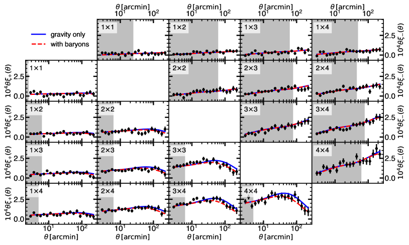
The catalogue of source galaxies is split into 4 broad redshift bins, roughly equi-populated between $z=[0,1.5]$ (the maximum nominal redshift is at $z=3$, although after $z=1.5$ the number density is very low). The 2 shear correlation functions, $\xi_{\pm}$, are measured in 20 logarithmic angular bins between 2.5 and 250 arcminutes. Joining auto and cross-correlations for both $\xi_{+}$ and $\xi_{-}$, we have a total of 400 data points, reduced to 227 when considering DES scale cuts. The covariance is obtained analytically by summing the Gaussian contribution, the 4-point connected part, the super-sample contribution, the survey geometrical effects, and the shape noise (Friedrich et al., 2021). We show our data vector in Fig. 1, where we highlight with grey bands the data points removed by the DES scale cuts.

3 Model

3.1 Cosmic shear

We obtain the shear correlation functions in the redshift bins $i,j$ $\xi^{i,j}_{\rm\pm}(\theta)$ by decomposing the shear field in E and B modes and combining the angular power spectra as

$$\begin{split}\xi^{i,j}_{\rm\pm}(\theta)=\sum\limits_{\ell}\frac{2\ell+1}{2\pi\ell^{2}\,(\ell+1)^{2}}\left[G^{+}_{\ell,2}(\cos\theta)\pm G^{-}_{\ell,2}(\cos\theta)\right]\\ \times\left[C^{i,j}_{\rm EE}(\ell)\pm C^{i,j}_{\rm BB}(\ell)\right]\end{split}$$ (1)

(Crittenden et al., 2002; Schneider et al., 2002; Krause et al., 2021). The $G^{\pm}_{\ell,2}$ functions are defined from the Legendre polynomials following Stebbins (1996). We compute efficiently Eq.1 by using the Fast Fourier Transforms FFTLog (Talman, 1978). We use the Limber approximation (Limber, 1953), which is shown to be accurate enough for DES Y3 data (Krause et al., 2021). We have explicitly checked that the post-Limber correction proposed by Kitching et al. (2017) does not impact significantly our results ($\leq 0.1\sigma$ in the cosmology inference).

The angular power spectra $C_{\rm EE}^{i,j}(\ell),C_{\rm BB}^{i,j}(\ell)$ are computed summing the relevant contributions, i.e.

$$C_{\rm EE}^{i,j}(\ell)=C_{\rm GG}^{i,j}(\ell)+C_{\rm II,EE}^{i,j}(\ell)+C_{\rm GI}^{i,j}+C_{\rm IG}^{j,i},$$ (2)

$$C_{\rm BB}^{i,j}(\ell)=C_{\rm II,BB}^{i,j}(\ell).$$ (3)

The purely gravitational signal is given by the term $C_{\rm GG}(\ell)$, which only contributes to E modes. Within a flat $\Lambda$CDM model, we can compute this term as:

$$C^{i,j}_{\rm GG}(\ell)=\int_{0}^{\chi_{\rm H}}\frac{g^{i}(\chi)g^{j}(\chi)}{\chi^{2}}P_{\rm GG}\left(\frac{\ell+1/2}{\chi},z(\chi)\right)d\chi,$$ (4)

where $P_{\rm GG}(k,z)$ is the matter power spectrum, $\chi$ is the comoving distance and $z$ the corresponding redshift. The lensing kernel $g^{i}(\chi)$ reads

$$g^{i}(\chi)=\frac{3}{2}\Omega_{\rm m}\left(\frac{H_{0}}{c}\right)^{2}\frac{\chi}{a}\int_{z(\chi)}^{z_{\rm H}}n^{i}(z^{\prime})\frac{\chi(z\prime)-\chi(z)}{\chi(z\prime)}dz\prime,$$ (5)

where $n^{i}(z)$ is the normalised galaxy redshift distribution in each $i$ bin (see Myles et al., 2021, for details on how these are obtained in the DES case), and $z_{\rm H}$ is the redshift of the Hubble sphere.

The other terms, $C_{\rm II,EE}(\ell)$ and $C_{\rm GI}$, are given by the intrinsic alignment of galaxies, and we recap them in the next section.

3.2 Intrinsic alignment

The measured shear signal includes the physical correlation of galaxy shapes in the sky, often referred to as the intrinsic alignment of galaxies. Within a flat $\Lambda$CDM framework and using the Limber approximation, the auto-correlation of the intrinsic alignment is given by

$$C^{i,j}_{II}(\ell)=\int_{0}^{\chi_{\rm H}}\frac{n^{i}n^{j}}{\chi^{2}}P_{\rm II}\left(\frac{\ell+1/2}{\chi},z\right)d\chi,$$ (6)

and the cross-correlation between gravitational shear and intrinsic alignment reads

$$C^{i,j}_{GI}(\ell)=\int_{0}^{\chi_{\rm H}}\frac{g^{i}n^{j}+g^{j}n^{i}}{\chi^{2}}P_{\rm GI}\left(\frac{\ell+1/2}{\chi},z\right)d\chi,$$ (7)

where for brevity we have omitted the dependence of $g,n$, and $z$ on $\chi$.

We implement two models of the intrinsic alignment of galaxies: the non-linear model (NLA, Bridle & King, 2007), and the more complex tidal alignment & tidal torque model (TATT, Blazek et al., 2019). The NLA model, with two free parameters, can be seen as a specific case of the more general TATT (5 free parameters).

Within NLA, the intrinsic alignment auto-correlation, and cross-correlation with cosmic shear are, respectively,

$$P_{\rm II}(k,z)=A_{1}(z)^{2}P_{\rm GG}(k,z),$$ (8)

$$P_{\rm GI}(k,z)=A_{1}(z)P_{\rm GG}(k,z),$$ (9)

with

$$A_{1}(z)=-a_{1}C_{1}\frac{\rho_{\rm crit}\Omega_{\rm m}}{D(z)}\left(\frac{1+z}{1+z_{0}}\right)^{\eta_{1}}.$$ (10)

Here, $C_{1}$ is a normalization constant typically set to $C_{1}=5\times 10^{-14}\,(h^{2}{\rm M_{\odot}Mpc^{3}})^{-2}$ (Hirata & Seljak, 2004; Bridle & King, 2007), $z_{0}=0.62$ is typically assumed in DES analysis (Secco et al., 2022; Amon et al., 2022), and $a_{1}$, $\eta_{1}$ are free parameters.

In the TATT model, we have instead

$$\begin{split}P_{\rm II,EE}=A_{1}^{2}P_{\rm GG}+2A_{1}A_{1,\delta}P_{\rm 0|0E}+A_{1,\delta}^{2}P_{\rm 0E|0E}\\ +A_{2}^{2}P_{\rm E2|E2}+2A_{1}A_{2}P_{0|E2}+2A_{1,\delta}A_{2}P_{0E|E2},\end{split}$$ (11)

$$P_{\rm II,BB}=A_{1,\delta}^{2}P_{\rm 0B|0B}+A_{2}^{2}P_{\rm B2|B2}+2A_{1,\delta}A_{2}P_{0B|B2},$$ (12)

and

$$P_{\rm GI}=A_{1}P_{\rm GG}+A_{1,\delta}P_{\rm 0|0E}+A_{2}P_{0|E2},$$ (13)

where for the sake of brevity we have omitted scale and redshift dependencies. The power spectra $P_{\rm 0|0E},P_{\rm 0E|0E},P_{\rm 0B|0B}$, etc., are computed within perturbation theory in Blazek et al. (2019), to which we refer for the details. We evaluate these power spectra using the public code FAST-PT (McEwen et al., 2016; Fang et al., 2017).

Following the convention of Secco et al. (2022); Amon et al. (2022), we define

$$A_{2}(z)=5a_{2}C_{1}\frac{\rho_{\rm crit}\Omega_{\rm m}}{D^{2}(z)}\left(\frac{1+z}{1+z_{0}}\right)^{\eta_{2}},$$ (14)

$$A_{1,\delta}(z)=b_{\rm TA}A_{1}(z).$$ (15)

We therefore have the additional free parameters $a_{2}$, $\eta_{2}$, $b_{\rm TA}$. When fixing $a_{2}=0$ and $b_{\rm TA}=0$, TATT reduces to NLA.

There is no consensus on the regime of validity of NLA and TATT (see e.g. Samuroff et al., 2022). Previous works on DES data have constrained the amplitude parameters of the intrinsic alignment, $a_{1}$,$a_{2}$, of the GOLD catalogue to be consistent with zero (Secco et al., 2022; Amon et al., 2022; Abbott et al., 2022; Samuroff et al., 2022). Indeed, Bayesian evidence prefers a model with no intrinsic alignment at all, followed by the NLA model. TATT is disfavoured because of its relatively high number of parameters combined with a low signal compared to the cosmological one. This can be seen as a preference towards simpler intrinsic alignment models for DES data. Therefore, in this work, we employ NLA as our fiducial model. Nonetheless, since we are employing angular scales previously discarded, we repeat the full analysis with TATT to check the robustness of our inference.

3.3 Matter power spectrum

We evaluate the matter power spectrum $P_{\rm GG}(k,z)$ employing a series of Neural Network emulators from the BACCO Simulation project (Angulo et al., 2021). Specifically, the matter power spectrum is decomposed into three different components: a linear part given by perturbation theory, a non-linear boost function given by $N$-body simulations, and a baryonic correction given by a baryonification algorithm.

The linear component is a direct emulation of the Boltzmann solver CLASS (Lesgourgues, 2011), which speeds up the calculations by several orders of magnitude (Aricò et al., 2022) while introducing a negligible error. The non-linear boost function is built by interpolating results at more than 800 different cosmologies, obtained from 5 high-resolution $N$-body simulations of $\approx 2{\rm Gpc}$ and $4320^{3}$ particles, together with the methodology developed by Angulo & White (2010); Angulo & Hilbert (2015); Zennaro et al. (2019); Angulo et al. (2021); Contreras et al. (2020). This algorithm manipulates the output of a simulation to mimic the expected particle distribution in a very wide cosmological space, with an accuracy of $3\%$ in the power spectrum at $k\sim 5h\,{\rm Mpc}^{-1}$ in $\Lambda$CDM including massive neutrinos (Contreras et al., 2020; Angulo et al., 2021). Finally, the baryonic correction is computed by applying a baryonification algorithm (Schneider & Teyssier, 2015; Aricò et al., 2020) to the $N$-body simulations.

These emulators have been collected into the public repository BACCOemu (Angulo et al., 2021; Aricò et al., 2021b; Aricò et al., 2022). Here, we use an updated version of the public emulators, which extends the non-linear boost functions from scales $k\leq 5h\,{\rm Mpc}^{-1}$ to $k\leq 10h\,{\rm Mpc}^{-1}$ and from redshifts $z\leq 1.5$ to $z\leq 3$ by employing a suite of 5 higher-resolution $N$-body simulations ($L\approx 750{\rm Mpc}$ and $2288^{3}$ particles). The new emulator also features an updated version of the cosmology rescaling algorithm, including a new halo mass function and concentration-mass relation (Ondaro-Mallea et al., 2022; López-Cano et al., 2022) which improves its accuracy. Moreover, the cosmological parameter space has been expanded thanks to the addition of a suite of 35 new simulations, so that encapsulate the priors used here. The only exception is the cold matter cosmic density, $\Omega_{\rm c}$, which nonetheless has been extended from $[0.23,0.4]$ to $[0.15,0.47]$ (we extrapolate with HALOFIT outside of these boundaries ). We show a comparison between HALOFIT and BACCOemu in App. A, and we refer to Zennaro et al. (in prep.) for further details and validation.

Cosmology
$\Omega_{\rm m}$	$[0.1,0.7]$
$A_{\rm s}$	$[5\times 10^{-10},5\times 10^{-9}]$
$h$	$[0.55,0.90]$
$\Omega_{\rm b}$	$[0.03,0.07]$
$n_{\rm s}$	$[0.87,1.07]$
$M_{\nu}$	$[0.0559,0.400]$ eV
Baryons
$\log{M_{\rm c}}$	$[9.0,15.0]$ $\log(h^{-1}{\rm M_{\odot}})$
$\log{\eta}$	$[-0.7,0.7]$
$\log{\beta}$	$[-1.0,0.7]$
$\log M_{z0,\rm cen}$	$[9.0,13.0]$ $\log(h^{-1}{\rm M_{\odot}})$
$\log{\theta_{\rm inn}}$	$[-2.00,-0.53]$
$\log{\theta_{\rm out}}$	$[-0.48,0.00]$
$\log{M_{\rm inn}}$	$[9.0,13.5]$ $\log(h^{-1}{\rm M_{\odot}})$
Intrinsic Alignment
$a_{1}$	$[-5,5]$
$\eta_{1}$	$[-5,5]$
$a_{2}$	$[-5,5]$
$\eta_{2}$	$[-5,5]$
$b_{\rm ta}$	$[0,2]$
Photo-z shift
$\Delta z_{\rm s}^{1}$	$\mathcal{N}(0.000,0.018)$
$\Delta z_{\rm s}^{2}$	$\mathcal{N}(0.000,0.015)$
$\Delta z_{\rm s}^{3}$	$\mathcal{N}(0.000,0.011)$
$\Delta z_{\rm s}^{4}$	$\mathcal{N}(0.000,0.017)$
Shear calibration
$m^{1}$	$\mathcal{N}(-0.0063,0.0091)$
$m^{2}$	$\mathcal{N}(-0.0198,0.0078)$
$m^{3}$	$\mathcal{N}(-0.0241,0.0076)$
$m^{4}$	$\mathcal{N}(-0.0369,0.0076)$

Table 1: Priors on the free parameters employed in our Bayesian analyses. The intrinsic alignment parameters $a_{2}$, $\eta_{2}$, $b_{\rm ta}$ are fixed to 0 in our fiducial run. We also impose a prior on the combination of parameters $\Omega_{\rm b}h^{2}\in[0.009,0.040]$.

3.4 Baryonic effects

We model the baryonic processes that impact the cosmic density field with a baryonification scheme (Schneider & Teyssier, 2015; Aricò et al., 2020). The baryonification, or Baryon Correction Model (BCM), displaces the particles of a gravity-only simulation according to analytical corrections to take into account the effects of different baryonic processes on the density field. In this framework, haloes are assumed to be constituted by galaxies, gas in hydrostatic equilibrium, and dark matter. A given fraction of the gas is expelled from the haloes by accreting supermassive black holes, and the dark matter back-reacts on the baryon gravitational potential with a quasi-adiabatic relaxation. The BCM has been proven flexible enough to reproduce the 2-point and 3-point statistics of several hydrodynamical simulations (Aricò et al., 2021a; Giri & Schneider, 2021), and has been used to analyse cosmic shear data (Schneider et al., 2022; Chen et al., 2023).

In this work, we employ the emulator of the BCM suppression in the matter power spectrum described in Aricò et al. (2020). The emulator fully captures the degeneracies between astrophysical processes and cosmology, while being accurate at per cent level (Aricò et al., 2021b). It has a total of 15 free parameters, 7 to describe the baryonic processes, plus 8 for cosmology. We further test the accuracy of the BCM emulator in the modelling of DES Y3 cosmic shear analysis in App. B, where we compare the BCM against the hydrodynamical simulation BAHAMAS (McCarthy et al., 2017; McCarthy et al., 2018).

Figure 2: Comparison between the posterior distribution on $S_{8}\equiv\sigma_{8}\sqrt{\Omega_{m}/0.3}$ and $\Omega_{m}$ obtained using CosmoSIS (employed by the DES Collaboration) and our pipeline, embedded in the BACCO library. For this comparison, both cases compute the nonlinear matter power spectrum using HALOFIT. The intrinsic alignment model used is NLA, without the contribution of shear ratios. Here and throughout this paper, we always show $1\sigma$ and $2\sigma$ credible levels (we note that DES Collaboration papers typically display $68\%$ and $95\%$ credible levels instead).

The cosmological parameter space in which the BCM emulator has been trained is smaller with respect to the DES priors. Thus, when sampling a cosmological model that lies outside the emulator space, we set the cosmological parameters of the baryonic response to the closest cosmology available. Additionally, we explicitly set the (cold) cosmic baryon fraction, $\Omega_{\rm b}/\Omega_{\rm cdm+b}$, to the closest available value. We expect this to be a good approximation because i) the $1-\sigma$ region obtained analysing only the large scales of DES broadly fits into the emulator priors; ii) the baryonic feedback is mainly dependent on the (cold) cosmic baryon fraction, which is reasonably well covered by our emulator ($\Omega_{\rm b}/\Omega_{\rm cdm+b}\in[0.1,0.26]$, more than $98\%$ of the posterior samples in our fiducial run falls within this interval).

Our BCM emulator has been previously applied to DES Y3 data in Chen et al. (2023) to constrain the impact of astrophysical feedback. They used small-scales DES Y3 shear measurements to constrain $M_{\rm c}$ – the baryonic parameter data is most sensitive to. That is, the characteristic halo mass ($M_{200,\rm crit}$ expressed in $h^{-1}{\rm M_{\odot}}$) in which half of the cosmic gas fraction is expelled from the halo by astrophysical processes. Chen et al. (2023) find that $\log M_{\rm c}=14.12^{+0.62}_{-0.37}$. In the analysis, the cosmology was varied within a prior given by the posterior provided by the 3x2pt analysis of DES Y3, that is the combination of cosmic shear with galaxy clustering and galaxy-galaxy lensing (Abbott et al., 2022).

The other free parameters of the BCM describe the shape of the density profile of the hot gas ($\theta_{\rm inn}$,$\theta_{\rm out}$,$M_{\rm inn}$), the galaxy-halo mass ratio ($M_{z0,\rm cen}$), the AGN feedback range $\eta$, and the gas fraction - halo mass slope ($\beta$). We refer the reader to Aricò et al. (2021a, b) for further details.

Here, we set free all the BCM parameters to avoid relying on a specific hydrodynamical simulation. We also explicitly test the impact of fixing all the BCM parameters but $M_{\rm c}$, as done in Chen et al. (2023).

Model	$\chi^{2}/{d.o.f.(N_{\rm free})}$		$\chi^{2}/{d.o.f.(N_{\rm eff})}$
	DES scale cuts	all scales	DES scale cuts	all scales
NLA BCM7 (fiducial)	226.98/204=1.11	414.14/377=1.1	226.98/224.69=1.01	414.14/397.16=1.04
NLA GrO	227.98/211=1.08	416.46/384=1.08	227.98/224.63=1.01	416.46/397.37=1.05
NLA BCM1	227.58/210=1.08	414.23/383=1.08	227.58/224.61=1.01	414.23/397.11=1.04
NLA BCM-extreme	227.24/211=1.08	419.03/384=1.09	227.24/224.6=1.01	419.03/397.77=1.05
TATT BCM7	226.28/201=1.13	411.22/374=1.1	226.28/224.14=1.01	411.22/396.21=1.04
TATT GrO	226.37/208=1.09	410.66/381=1.08	226.37/224.28=1.01	410.66/396.16=1.04
TATT BCM1	225.28/207=1.09	407.65/380=1.07	225.28/223.87=1.01	407.65/396.35=1.03
TATT BCM-extreme	227.2/208=1.09	408.69/381=1.07	227.2/223.77=1.02	408.69/396.37=1.03

Table 2: Goodness of fits of our models given the DES Y3 data vector. We calculate the degrees of freedom ($d.o.f.$) by subtracting the number of parameters $N_{\theta}$ from the number of data points ($N_{\mathcal{D}}$). We use as $N_{\theta}$ either the number of free parameters $N_{\rm free}$, or the number of effective parameters $N_{\rm eff}$ as defined in Raveri & Hu (2019). We explore different models, with NLA or TATT intrinsic alignment, gravity-only, or applying a baryonification with 1 or 7 free parameters (BCM1 & BCM7, respectively). We also include a model with an extreme implementation of AGN feedback.

3.5 Nuisance Parameters

Following the DES Collaboration, we model the uncertainties on the photometric redshift estimate of source galaxies as a shift in the redshift distributions in each redshift bin $\Delta z_{\rm s}^{i}$. Furthermore, we model the unaccounted effects of the shape calibration and blending of the galaxy shapes with a multiplicative bias independent for each redshift bin, $m^{i}$. For both, photometric errors and shear bias, we employ the informative priors used in Secco et al. (2022); Amon et al. (2022).

3.6 Pipeline

For this work, we have implemented from scratch a WL analysis pipeline. The pipeline is interfaced with the cosmology library BACCO (Angulo et al., in prep.) and the BACCOemu emulators. It is written in python, with a multi-threaded C core for the most computationally-demanding functions. As input, the pipeline takes a series of parameters (including cosmological, astrophysical, intrinsic alignment, photometric errors, and shear bias parameters), and it outputs the predicted shear correlation functions.

We perform the Bayesian analysis with a nested sampling algorithm, the public code POLYCHORD (Handley et al., 2015). We follow the guidelines of Lemos et al. (2022) (Tab. 3) and use their ”Publication quality” setting, which features 500 live points and a tolerance of 0.01. We assume a Gaussian likelihood with a covariance matrix provided by the DES collaboration.

In contrast to the official DES analysis, we choose not to include the so-called shear ratios (Sánchez et al., 2022; Amon et al., 2022). Defined in Sánchez et al. (2022), shear ratios measure the galaxy-galaxy lensing produced by the same lenses with different source galaxies samples. They found that, even at the smallest angular scales measured by DES Y3, these ratios are robust to changes in cosmology, baryonic processes, and galaxy bias, but highly sensitive to the source galaxy redshift distribution and intrinsic alignment. Despite the potential benefits, we opt for focusing only on shear data for two reasons: i) we avoid complications such as the modelling of galaxy bias, that we should coherently include in our current framework ii) we can better isolate the information on intrinsic alignment and redshift distributions coming from the small scales of cosmic shear.

Figure 3: $1\sigma$ and $2\sigma$ credible levels on $S_{8}$ and $\Omega_{\rm m}$ obtained using BACCO, considering only gravity in structure formation (left panel) and including baryonic effects (right panel). Black solid lines refer to runs with the application of scale cuts, and red solid lines to runs where all scales are used. The black dotted line in the right panel shows for reference the results of the gravity-only model with scale cuts.

We generally use the same priors as the official DES analyses (Secco et al., 2022; Amon et al., 2022; Abbott et al., 2022), except for the upper boundary of $\Omega_{\rm m}$ which is 0.7 in our analysis instead of 0.9, of $h$ which is 0.9 instead of 0.91, and of the sum of neutrino masses $M_{\nu}$ that is 0.4 instead of 0.6, to fit in the parameter space of our emulator. We have checked with HALOFIT that these new priors do not significantly impact our final results. Specifically, we only detect a small bias of less than $0.1\sigma$ on the cosmological constraints, given by the different prior on $M_{\nu}$. This is in broad agreement with what was found in (Secco et al., 2022; Amon et al., 2022) when fixing the sum on neutrino masses. The priors on baryonic parameters are those discussed in Aricò et al. (2021b), chosen to be wide enough to encompass X-ray observations and hydrodynamical simulations.

We summarise the priors we use in Tab. 1. In our fiducial run, we use the NLA intrinsic alignment model, i.e. $a_{2}=\eta_{2}=b_{\rm ta}=0$. We also include an extra flat prior $\Omega_{\rm b}h^{2}\leq 0.04$ given by Big Bang Nucleosynthesis (Beringer et al., 2012), analogously to that adopted in CosmoSIS and by the DES Collaboration (Zuntz et al., 2015; Abbott et al., 2022).

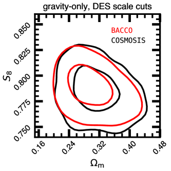
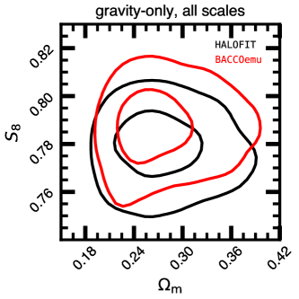
We have validated our pipeline by performing a model comparison with the public codes implemented in CosmoSIS (Zuntz et al., 2015) and Core Cosmology Library (CCL, Chisari et al., 2019), finding an excellent agreement between the three. We have also performed a test run employing HALOFIT (Takahashi et al., 2012) and NLA, and using the official DES scale cuts. We compare these results with the chains run with the DES pipeline and CosmoSIS in Fig. 2, where we show for convenience only the $\Omega_{\rm m}-S_{8}$ plane. Throughout the paper, we use the definition $S_{8}\equiv\sigma_{8}\sqrt{\Omega_{\rm m}/0.3}$. We find a difference between the two pipelines of about $0.1\sigma$, a very good agreement when considering all the different details of the implementation (e.g. binning, numerical accuracy, interpolation, emulators, etc.). Although not shown here, we have checked that the agreement holds true for all the model’s free parameters.

As further validation of our pipeline, and in order to check for possible biases introduced when analysing the smallest scales used in this work, we compute the $\chi^{2}$ values obtained using an independent, state-of-the-art model, and compare them with ours. We use a model composed by i) EuclidEmulator2 (Euclid Collaboration et al., 2020) for the non-linear matter power spectrum; ii) the baryonic suppression measured in the BAHAMAS suite of hydrodynamical simulations (McCarthy et al., 2017); iii) the TATT intrinsic alignment of galaxies (Blazek et al., 2019).

Comparing this model with our fiducial one for different cosmological and baryonic parameters (Planck and DES Y3 best-fitting cosmologies (Planck Collaboration et al., 2018; Amon et al., 2022; Secco et al., 2022), BAHAMAS low, reference, and high AGN suppressions), we find fractional differences in $\chi^{2}$ below 1%. By contrast, the difference in $\chi^{2}$ between baryonic modelling and gravity-only is around 5-15%. The difference in $\chi^{2}$ between NLA and TATT is highly dependent on the value of the TATT parameters ($a_{2}$, $b_{\rm TA}$), and can be lower than $1\%$ and larger than $20\%$. Apriori, we do not know the amplitudes of TATT for a survey like DES, although previous studies point toward low amplitudes (and thus smaller $\chi^{2}$ differences). Therefore, we compare a posteriori the results obtained with NLA and TATT in App. E.

Finally, we note that with our pipeline we evaluate a likelihood in less than 0.5 seconds on a common laptop, whereas it takes about 8 seconds to run a standard DES Y3 cosmic shear likelihood evaluation with CosmoSIS.

4 Analysis

In this section, we employ the pipeline described and validated in §3 to obtain constraints on cosmology, baryonic physics, and intrinsic alignment of galaxies. We explore different levels of complexity in our model and study their impact on cosmology inference. We will focus on the derived cosmological parameter $S_{8}$, and on $\Omega_{\rm m}$. When showing the credible levels in the $S_{8}-\Omega_{\rm m}$ plane, we display the $1\sigma$ and $2\sigma$ levels (i.e. 39% and 86% in 2D), as opposed to $68\%$ and $95\%$ normally shown in DES papers, to visually help the assessment of tensions between different models and datasets. Unless stated otherwise, we quote all our constraints as the mode of the 1D marginalised posterior, plus and minus the respective 34th percentiles. We caution against directly comparing with the official DES constraints, which typically report the mean of the marginalised posterior. To help the comparison, we have reanalysed the DES Collaboration chains with the same routine we use for our chains (ChainConsumer, Hinton, 2016). We report in Tab. 3 the constraints obtained with the mode and in Tab. 4 with the median of the posteriors, and their respective 34th percentiles.

4.1 Constraints on cosmology and goodness of fit

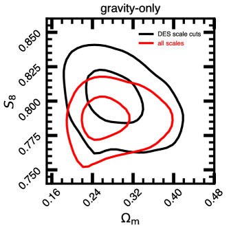
In Fig. 3 we show the posterior distribution functions of the cosmological parameters $S_{8}$ and $\Omega_{\rm m}$ assuming only gravitational interactions (left panel) and including our fiducial 7-parameters baryonic model (right panel). In each case, we display our results when applying DES scale cuts (black lines) and when employing all scales (red). When using our fiducial model, and analysing all the angular scales available, we obtain $S_{8}=0.799^{+0.023}_{-0.015}$ and $\Omega_{\rm m}=0.252^{+0.066}_{-0.030}$. In Tab. 3 we report the constraints on $S_{8}$ and $\Omega_{\rm m}$ obtained with different modelling choices, whereas in App. C we show the posteriors of all the free cosmological parameters in our fiducial run.

Both the models with and without baryons provide a statistically good fit of the data, as shown in Fig. 1 (red solid and blue dash lines, respectively). More quantitatively, we report the goodness of the fit for all our models in Tab. 2, defined with the reduced $\chi^{2}$:

$$\hat{\chi}^{2}=\frac{\chi^{2}}{d.o.f.}=\frac{(\mathcal{D}-\mathcal{M})^{\rm T}\mathcal{C}^{-1}(\mathcal{D}-\mathcal{M})}{N_{\mathcal{D}}-N_{\theta}},$$ (16)

where $\mathcal{D}$ is our data vector, $\mathcal{M}$ is our model, $\mathcal{C}$ the covariance, and the degrees of freedom ($d.o.f.$) are found by subtracting the number of parameters $N_{\theta}$ from the number of data points ($N_{\mathcal{D}}$). We use as $N_{\theta}$ either the number of free parameters $N_{\rm free}$, or the number of effective parameters $N_{\rm eff}$ as defined in Raveri & Hu (2019). When using $N_{\rm free}$, we find a slightly higher $\hat{\chi}^{2}$ in the case with baryons with respect to the gravity-only ($\hat{\chi}^{2}=1.1$ and $\hat{\chi}^{2}=1.08$, respectively), due to the 7 extra free parameters. When using $N_{\rm eff}$ we find instead $\hat{\chi}^{2}=1.04$ with baryons and $\hat{\chi}^{2}=1.05$ in the gravity-only case, which corresponds to $p$-values of $0.27$ and $0.24$, respectively. Nonetheless, the posteriors in the $S_{8}$-$\Omega_{\rm m}$ plane are quite different, the gravity-only one being tighter and shifted towards lower values of $S_{8}$.

4.2 Cosmological information at small scales

Although the DES measurements of the shear correlation functions get to angles as small as $2.5$ arcminutes, the DES Collaboration has so far refrained from modelling such small scales because of possible biases in the cosmology inference due to the effects of baryons. In particular, they have set different angular scale cuts for $\xi_{+}$ and $\xi_{-}$ and each redshift bin.

The DES scale cuts are chosen such that the difference in $\chi^{2}$ between analyses carried on with a given synthetic data vector and the same data vector contaminated with the baryonic effects predicted by the hydrodynamical simulation OWLS-AGN (Schaye et al., 2010) is lower than a given threshold (for more details, see e.g. Krause et al., 2021). This results in retaining 227 data points over 400 (166 in $\xi_{+}$, 61 in $\xi_{-})$.

To quantify the amount of cosmological information loss when discarding in the analysis the small angular separations, we run our pipeline with and without these scale cuts. First, we neglect the effects of baryonic physics to get a sense of the improvement in the cosmological constraints in an ideal scenario, even if likely the constraints will be biased. We show the $1\sigma$ and $2\sigma$ credible levels of $S_{8}$ and $\Omega_{\rm m}$ in the left panel of Fig. 3. Adopting the DES scale cuts, we obtain $S_{8}=0.802^{+0.019}_{-0.021}$, whereas including smaller scales we find $0.785^{+0.017}_{-0.012}$, a constraint $30\%$ tighter. This can be seen as the upper limit on the cosmological information that we can potentially gain when modelling the small scales. Note, however, that this figure is specific to DES Y3 data, since it depends on the statistical accuracy with which small scales are measured. For surveys with a higher number density of background galaxies, better photometry and angular resolution, we expect the gains to be more substantial.

When including small scales, we see how the $S_{8}$ posterior shifts by about $0.5\sigma$ towards lower values. This is likely caused by baryonic processes: the lack of modelling of the suppression in the matter power spectrum caused by baryons could be compensated by a lower inferred value of $\sigma_{8}$ and $\Omega_{\rm m}$. Hence, to be able to exploit the data on small scales, it is necessary to explicitly model the role of baryonic physics.

Figure 4: Posterior distribution functions of $\log M_{\rm c}$ obtained in our fiducial run using all angular scales (red) and applying scale cuts (blue). We compare against the posterior obtained by Chen et al. (2023) using only small scales, fixing 6 baryonic parameters and applying a prior on cosmology given by the 3x2pt analysis of DES Y3 (Abbott et al., 2022).

Figure 5: $1\sigma$ credibility region of the suppression in the matter power spectrum at $z=0$ caused by baryons, inferred by the BCM model with DES Y3 data (grey shaded area). We display the ratio between the matter power spectrum affected by baryonic processes over the gravity-only one. For comparison, we show the BCM models obtained in Aricò et al. (2021b), fitting several state-of-the-art hydrodynamical simulations referenced in the main text, according to the legend.

4.3 Impact of baryons

Baryonic processes like gas cooling, galaxy formation, and active galactic nuclei (AGN) modify the cosmic matter power spectrum in a nontrivial way. The scales and amplitudes of their effects are currently debated, and can potentially affect the cosmology inference, if not properly taken into account.

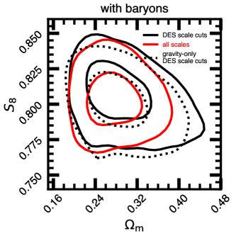
In this work, we model the impact of baryonic processes on the cosmic shear via the baryonification emulator described in §3.4. We show the constraints on $S_{8}$ and $\Omega_{\rm m}$ that we obtain with and without scale cuts in the right panel of Fig. 3. We obtain $S_{8}=0.807^{+0.020}_{-0.022}$ with the DES scale cuts and $S_{8}=0.799^{+0.023}_{-0.015}$ without scale cuts. Interestingly, when applying the scale cuts, the marginalisation over baryons does not broaden significantly the $S_{8}$ constraints, although it slightly shifts the posterior towards high $S_{8}$, by $0.2\sigma$. This might be caused by a residual signal of baryonic effects in the data vector even after imposing the scale cuts, or it could also be a projection effect given by the unconstrained baryonic parameters.

The marginalisation over 7 free baryonic parameters has significantly more impact when analysing all the angular scales: we find the constraint on $S_{8}$ $\approx 24\%$ weaker with respect to the gravity-only case, degrading part of the extra cosmological information contained in the small scales. However, we find no bias in the $S_{8}$-$\Omega_{\rm m}$ introduced by the addition of the small scales in the analysis. Moreover, we gain cosmological information when marginalising over baryons and going to smaller scales. When comparing the constraints we obtain with and without the angular scale cuts, we find $S_{8}$ and $\Omega_{\rm m}$ that are $10\%$ and $22\%$ tighter, respectively.

This finding validates the robustness of the modelling of baryonic processes at all the scales employed in this work. We note that the marginalisation over 7 free baryonic parameters is a conservative choice, given that, as shown in App. D, only one of these parameters is strongly constrained by our data.

Therefore, adding extra information on baryonic processes, either with constraints from external datasets or educated guesses from hydrodynamical simulations, could help recover, at least partially, the cosmological information lost in the marginalisation. For instance, we could fix the unconstrained baryonic parameters to a value inferred with hydrodynamical simulations, analogously to Chen et al. (2023). By setting all the parameters except $M_{\rm c}$ to the best-fitting parameters of the matter power spectrum of the hydrodynamical simulations BAHAMAS at $z=0$, we obtain $S_{8}=0.799^{+0.017}_{-0.017}$, in perfect agreement with our fiducial case, but $15\%$ tighter and with a better $\hat{\chi}^{2}$.

Figure 6: Degeneracy between $S_{8}$ and $\log M_{\rm c}$, displaying the $1\sigma$ and $2\sigma$ credible levels (red), and using all angular scales. For comparison, we show as a horizontal band the $1\sigma$ constraints on $S_{8}$ obtained analysing all angular scales without modelling baryons (blue), and using the Planck TT+TE+EE+lowE posterior obtained by the DES Collaboration (black, Planck Collaboration et al., 2018; Secco et al., 2022).

4.4 Constraints on baryons

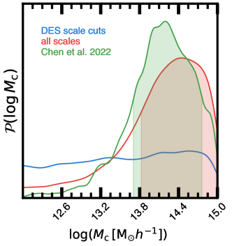
By including in our analysis all the angular scales available, we are able to constrain the astrophysical processes which modify the gravitational evolution of the cosmic density field. In particular, it has been shown that the suppression in the matter power spectrum is proportional to the gas fraction expelled from haloes by baryonic feedback processes (Schneider & Teyssier, 2015; van Daalen et al., 2020). We parametrise this fraction with $M_{\rm c}$, the characteristic halo mass for which half of the gas is depleted.

Figure 7: $1\sigma$ and $2\sigma$ credible levels on $S_{8}$ and $\Omega_{\rm m}$ using the Planck TT+TE+EE+lowE posteriors of the DES Collaboration (black, Planck Collaboration et al., 2018; Secco et al., 2022) and DES Y3 cosmic shear data, analysing all the angular scales either with our fiducial model (red) or without modelling baryons (blue), obtained in this work.

In Fig. 4 we show our constraints on $\log M_{\rm c}$ when including or not the small scales removed in the official DES analysis. When we apply the DES scale cuts, as expected, $\log M_{\rm c}$ is unconstrained, even if the data might have a residual sensitivity to baryonic effects, with higher values of $M_{\rm c}$ slightly preferred (blue line). When we analyse all the angular scales, we obtain a tight constraint $\log M_{\rm c}=14.38^{+0.60}_{-0.56}\,[\log(h^{-1}{\rm M_{\odot}})]$ (red line).

We find an excellent agreement between our estimate of $M_{c}$ and that obtained by Chen et al. (2023) (green line) which employed the same model as ours. However, our constraints are slightly weaker due to the different assumptions in the two analyses: first, Chen et al. (2023) employ an informative prior on cosmology, with all cosmological parameters fixed except for $\sigma_{8}$ and $\Omega_{\rm m}$, given by the 3x2pt analysis of DES Y3. Second, Chen et al. (2023) used only the data points with angles smaller than the DES scale cuts, a TATT intrinsic alignment model, and they fixed all the baryonic parameters except $M_{\rm c}$ to the best-fitting values of the hydrodynamical simulation OWLS-AGN (Schaye et al., 2010). The different priors in cosmology (i.e. the extra information on cosmology retrieved by galaxy clustering, galaxy-galaxy lensing, and shear ratios) have likely the largest impact.

We observe that the posterior of $\log M_{\rm c}$ hits the boundary of its prior, at $\log M_{\rm c}=15\,[\log(h^{-1}{\rm M_{\odot}})]$. This prior has been chosen to broadly encompass the current measurement of gas fractions in galaxy clusters measured in $X$-ray (Vikhlinin et al., 2006; Arnaud et al., 2007; Sun et al., 2009; Giodini et al., 2009; Gonzalez et al., 2013), as well as the prediction of hydrodynamical simulations McCarthy et al. (2017); McCarthy et al. (2018). Therefore, we note that we are explicitly adding to our analysis prior information on the quantity of gas inside haloes, which cannot be lower than half the cosmic baryon fraction for haloes with mass $M_{\rm 200,c}=10^{15}h^{-1}{\rm M_{\odot}}$. Even if we argue that the prior on $M_{\rm c}$ is broad enough given X-ray data, we plan to build the next version of the baryonic emulator extending the prior $M_{\rm c}$ to higher values, to better cover the parameter space allowed by WL-only data.
The remaining 6 free baryonic parameters are unconstrained, and we show their posteriors in App. D.
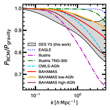
Finally, in Fig. 5 we show the estimated suppression in the matter power spectrum at $z=0$. Specifically, we show the $1\sigma$ credible interval obtained taking into account the full posterior of the free cosmological and baryonic parameters in our analysis. We compare it to the BCM best-fitting models to several state-of-the-art hydrodynamical simulations, obtained in Aricò et al. (2021b): EAGLE (Schaye et al., 2015; Crain et al., 2015; McAlpine et al., 2016), Illustris (Vogelsberger et al., 2014), Illustris TNG (Pillepich et al., 2018; Springel et al., 2018), OWLS-AGN (Schaye et al., 2010), and BAHAMAS (McCarthy et al., 2017; McCarthy et al., 2018). We infer a suppression of about $10\%$ at $k=2h\,{\rm Mpc}^{-1}$, in broad agreement with the BAHAMAS suite and OWLS-AGN, but stronger than EAGLE and Illustris TNG and milder than Illustris. This finding is in perfect agreement with Chen et al. (2023), although since we let free all the baryonic parameters, our model is more flexible e.g. at large scales (dominated by $\eta$, i.e. the distance range of the AGN feedback) and small scales (modulated by $M_{\rm z0,cen}$ and $\theta_{\rm inn}$, which regulate the galaxy-halo mass relation and inner shape of the gas, respectively).

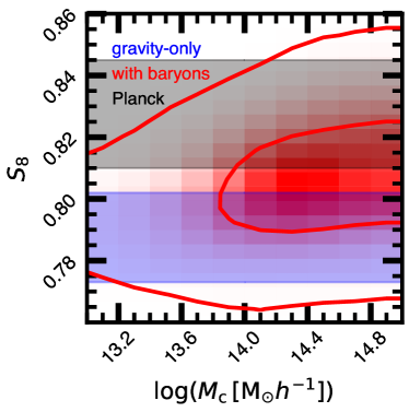
4.5 Correlation between cosmological and baryonic parameters

Constraints on cosmology and baryonic physics are not independent. For instance, the impact of AGN on the matter field depends on the amount of gas affected by feedback from supermassive black holes, and therefore on the cosmic baryon fraction $\Omega_{\rm b}/\Omega_{\rm m}$. Also, the amplitude of the linear density fluctuations, $\sigma_{8}$, affects in a minor and less trivial way the baryonic feedback (Schneider et al., 2020; Aricò et al., 2021b). We can thus expect to find a correlation between $S_{8}$ and $M_{\rm c}$. We show the $1\sigma$ and $2\sigma$ credible levels of these two parameters in Fig. 6. Indeed, we observe a weak but clear degeneracy, so that at high values of $M_{\rm c}$ correspond high values of $S_{8}$. For comparison, we display as bands the Planck TT+TE+EE+lowE $1\sigma$ intervals on $S_{8}$ obtained by the DES Collaboration (Planck Collaboration et al., 2018; Secco et al., 2022), and our gravity-only analysis with all the angular scales. Following the degeneracy direction in $S_{8}-M_{\rm c}$, we can see how lower values of $M_{\rm c}$ agree with the $S_{8}$ values obtained by our DES gravity-only analysis, whereas going towards high values of $M_{\rm c}$ the value of $S_{8}$ becomes more compatible with Planck. We study the implications in the context of the so-called $S_{8}$ tension in §5, but before, we discuss the constraints on intrinsic alignments from our small-scales analysis.

4.6 Constraints on intrinsic alignment

Our model allows us to constrain the intrinsic alignment of galaxies taking advantage of all the angular scales of DES Y3. With the NLA model and using DES angular scale cuts, we find $a_{1}=0.22^{+0.48}_{-0.30}$ and $\eta_{1}=4.11^{+0.86}_{-3.50}$. Interestingly, including small scales results in a tighter constrain on $\eta_{1}$ but not on $a_{1}$: removing scale cuts we infer $a_{1}=0.09^{+0.58}_{-0.25}$ and $\eta_{1}=4.50^{+0.48}_{-3.35}$.

The NLA model seems to be sufficient to describe the full range of angular scales in DES. In fact, NLA is statistically preferred over TATT: we find a ratio of the Bayesian evidence $\mathcal{R}=\mathcal{Z}_{\rm NLA}/\mathcal{Z}_{\rm TATT}=3.0\pm 1.2$. This value indicates a moderate/substantial preference for NLA over TATT, according to the commonly used (and somewhat arbitrary) Jeffreys scale (Jeffreys, 1935). For comparison, we find that the baryonic model with 7 free parameters is preferred to the gravity-only with a $\mathcal{R}=1.5\pm 1.2$, and freeing only the baryonic parameter $M_{\rm c}$, $\mathcal{R}=5.14\pm 1.2$. Despite this, the goodness of the fit is marginally better with TATT, $\hat{\chi}^{2}=1.033$, with respect to NLA $\hat{\chi}^{2}=1.043$.

Our inferred amplitudes of TATT in the DES galaxy sample are very low and consistent with zero, in agreement with Secco et al. (2022); Amon et al. (2022). That means that the intrinsic alignment contribution is subdominant with respect to the cosmological signal, and that simpler models are statistically preferred. We find also internal degeneracies in TATT which produce a multi-modal posterior of the tidal torque amplitude. We further analyse and discuss the results obtained with TATT in App. E.

5 The $S_{8}$ tension

Model	$S_{8}$		$\Omega_{\rm m}$
This work	DES scale cuts	all scales	DES scale cuts	all scales
NLA BCM7 (fiducial)	$0.807^{+0.020}_{-0.022}$	$0.799^{+0.023}_{-0.015}$	$0.259^{+0.083}_{-0.040}$	$0.252^{+0.066}_{-0.030}$
NLA GrO	$0.802^{+0.019}_{-0.021}$	$0.785^{+0.017}_{-0.012}$	$0.253^{+0.084}_{-0.030}$	$0.249^{+0.061}_{-0.035}$
NLA BCM1	$0.803^{+0.019}_{-0.020}$	$0.799^{+0.017}_{-0.017}$	$0.262^{+0.073}_{-0.044}$	$0.253^{+0.066}_{-0.036}$
NLA BCM-extreme	$0.838^{+0.030}_{-0.022}$	$0.829^{+0.023}_{-0.022}$	$0.243^{+0.094}_{-0.025}$	$0.272^{+0.078}_{-0.036}$
TATT BCM7	$0.796^{+0.022}_{-0.028}$	$0.788^{+0.027}_{-0.035}$	$0.258^{+0.084}_{-0.031}$	$0.227^{+0.065}_{-0.029}$
TATT GrO	$0.794^{+0.021}_{-0.030}$	$0.755^{+0.028}_{-0.023}$	$0.248^{+0.076}_{-0.029}$	$0.253^{+0.057}_{-0.039}$
TATT BCM1	$0.791^{+0.027}_{-0.025}$	$0.790^{+0.022}_{-0.035}$	$0.252^{+0.073}_{-0.041}$	$0.235^{+0.052}_{-0.030}$
TATT BCM-extreme	$0.828^{+0.029}_{-0.032}$	$0.816^{+0.034}_{-0.030}$	$0.267^{+0.065}_{-0.052}$	$0.237^{+0.060}_{-0.031}$
DES Collaboration
DES NLA	$0.783^{+0.024}_{-0.022}$	-	$0.289^{+0.080}_{-0.045}$	-
DES NLA + SR	$0.775^{+0.017}_{-0.022}$	-	$0.291^{+0.042}_{-0.055}$	-
DES TATT	$0.767^{+0.030}_{-0.039}$	-	$0.270^{+0.071}_{-0.042}$	-
DES TATT + SR (fiducial)	$0.763^{+0.021}_{-0.026}$	-	$0.269^{+0.059}_{-0.044}$	-

Table 3: Constraints (mode of the 1D marginalised posteriors and respective 34th percentiles) on $S_{8}$ and $\Omega_{\rm m}$ obtained applying DES scale cuts and using all the angular scales. We explore different models, with NLA or TATT intrinsic alignment, gravity-only, or applying a baryonification with 1 or 7 free parameters (BCM1, BCM7, respectively). We also include a model with an extreme implementation of AGN feedback. We report for comparison the constraints we get analysing the DES Collaboration chains, with and without shear ratios (SR).

Figure 8: $S_{8}$ constraints obtained in this work with different analysis strategies of DES Y3 data, either applying the scale cuts (grey data points) or employing all the angular scales (red data points). We highlight our fiducial model by displaying a red band correspondent with its $1\sigma$ credible interval. We employ our baryonification (BCM) with 1 or 7 free parameters, or fix all the parameters to extreme baryonic feedback. This last model, dubbed BCM-extreme, is in tension with X-ray observations, and should be considered as an upper limit for baryonic effects. We also vary the intrinsic alignment model choosing either NLA or TATT. For comparison, in the lower part of the panel we display the constraints obtained from the DES Collaboration chains with scale cuts, adding or not the shear ratios (black data points, Secco et al., 2022; Amon et al., 2022; Abbott et al., 2022). Moreover, we include the external datasets specified in the legend (blue data points, Planck Collaboration et al., 2018; Asgari et al., 2021; Li et al., 2023; Philcox & Ivanov, 2022; Nunes & Vagnozzi, 2021; Madhavacheril et al., 2023), which we describe in more detail in the main text. We highlight with a blue band the $1\sigma$ region preferred by Planck.

In this section, we compare the cosmological constraints that we have obtained analysing the cosmic shear of DES Y3 against external datasets, in light of the so-called $S_{8}$ tension. We also compare our results with the official ones obtained by the DES Collaboration, and discuss the main differences in the analyses.

Throughout this section, we will quantify the tension among datasets or analyses by approximating the marginalised posteriors as Gaussian-distributed functions, and considering the mean and standard deviation following e.g. Heymans et al. (2021) (for a method that takes into account non-Gassianity, see e.g. Raveri & Doux, 2021).

5.1 Impact of different model assumptions on the $S_{8}$ tension

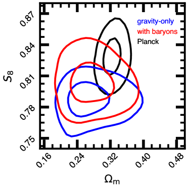
In Fig. 7 we compare our results against results from the analysis of Planck’s satellite data including temperature and polarization measurements (TT+TE+EE+lowE power spectra). Specifically, we use the chains made available by the DES Collaboration, where the Planck likelihood is sampled over the same prior-space used in the DES analysis (and therefore almost identical to ours). We also show our fiducial analysis (no scale cuts, explicit model for baryons, NLA for intrinsic alignments, and emulators for the matter power spectrum) as red lines, and the gravity-only case as blue lines.

We can see that our marginalised posteriors on $S_{8}$ are in $1.9\sigma$ tension in the gravity-only case compared to Planck. However, the tension reduces to $0.9\sigma$ when marginalising over baryonic effects. Therefore, our data suggest that at present Planck and DES Y3 are not statistically in tension. Additionally, the agreement between the data could potentially increase further if, for instance, external datasets (e.g. X-ray gas fraction) constrain the baryonic parameters to relatively strong feedback.

Combining such datasets is a non-trivial task, due to different systematics, e.g. hydrostatic mass bias and data covariances, and it is outside the scope of this work. However, this could be an interesting avenue to investigate in the future.

To explore further how the $S_{8}$ posterior is affected by the modelling of baryons, we consider two different scenarios. First, we fix all the baryonic parameters except for $M_{\rm c}$ to the best-fitting values of the matter power spectrum measured in the hydrodynamical simulation BAHAMAS at $z=0$. Second, to have a sense of what is the most extreme shift in $S_{8}$ that baryonic processes can cause, we set the baryonic parameters to the values that maximise the feedback allowed by our emulator. We note that these parameters are already ruled out by X-ray data, even if we find that they still provide a good fit to the DES Y3 cosmic shear data. We dubbed this model BCM-extreme.

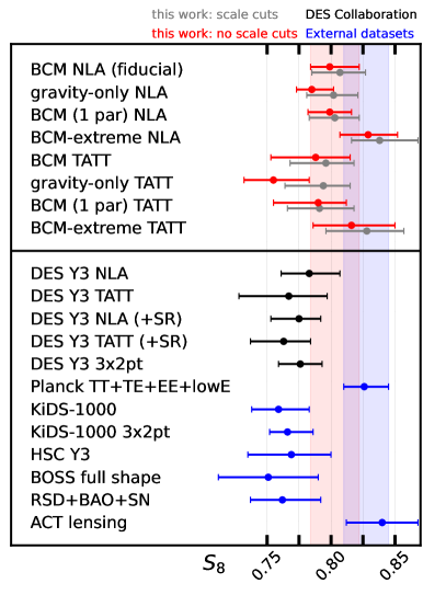
We summarise all our $S_{8}$ constraints in Fig. 8 and in Tab. 3. We note that the $S_{8}$ value inferred with and without scale cuts are generally in good mutual agreement, except for the gravity-only models where they present $0.5\sigma$ (with NLA) and $0.9\sigma$ (with TATT) shifts. In particular, our gravity-only analysis with DES scale cuts differs by less than $1\sigma$ from Planck, when using either NLA or TATT. We can conclude that DES angular scale cuts are reliably removing the baryonic effects, which must be accounted for only when analysing the full DES data vector. This is not true for scenarios with very high baryonic feedback. For example, in our BCM-extreme case, we find an excellent agreement between the DES Y3 cosmic shear and Planck (tension of $0.1\sigma$), both with and without scale cuts. However, we stress that this a very unlikely baryonic scenario, where all the gas within haloes up to $M=10^{15}h^{-1}{\rm M_{\odot}}$ has been pushed for tens of Mpc, and must be simply taken as an extreme upper limit of the impact of baryonic processes.

Finally, by comparing the $S_{8}$ values obtained by varying intrinsic alignment models, we observe in Fig. 8 that the $S_{8}$ posteriors are generally broader and shifted towards lower values when using TATT. This trend could be caused by internal degeneracies and projection effects of the TATT parameters, which are allowed to vary over a broad parameter space that is not physically motivated, as speculated also by Secco et al. (2022). We explore this in more detail in App. E.

Figure 9: Prior (black) and posteriors of the photo-z shift in the second tomographic bin $\Delta z_{\rm s}^{2}$, when using DES scale cuts (blue) and all angular scales (red). For comparison, we show the posteriors from the DES Collaboration chains, with scale cuts and the addition of the lensing shear ratios (green, Amon et al., 2022; Secco et al., 2022).

5.2 Comparison with the official DES Y3 analysis

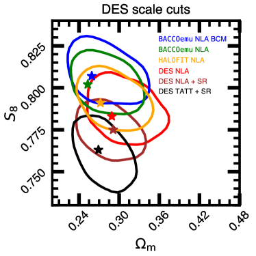
Our constraint on $S_{8}$ is systematically higher than that obtained with the same dataset by the DES Collaboration (Secco et al., 2022; Amon et al., 2022). Even when applying the DES scale cuts, our gravity-only results are $1.4\sigma$ away from those of the DES Collaboration. This is a significant discrepancy since both analyses use exactly the same shear correlation functions. We now explore the origin of this discrepancy.

In Fig. 10 we illustrate the impact of various modelling ingredients and choices in the $S_{8}-\Omega_{m}$ constraints. Lines show the $1\sigma$ credibility contours whereas stars highlight the mode of the marginalised posteriors. The official DES and our fiducial results are shown in black and blue, respectively. We now discuss specific differences in the analyses.

Intrinsic alignments: An important difference is the choice of the fiducial intrinsic alignment model. We estimate a shift toward high $S_{8}$ between $0.4\sigma$ and $0.7\sigma$ when using NLA instead of TATT, depending on modelling choices e.g. scale cuts, baryonic modelling, and shear ratios. As we have argued before (§4.6), although TATT is in principle a more complete description of intrinsic alignments, the additional complexity is not justified by the current data. This is the case for the DES analysis and scale cuts as well as for our approach including small scales.

Shear ratios: Another difference is that we do not employ the lensing shear ratios. In the DES analysis, excluding shear ratios increases $S_{8}$ by $\sim 0.1$ and $0.3\sigma$ when employing NLA and TATT, respectively. The shift is arguably caused by stronger constraints on the photo-z uncertainties and intrinsic alignment parameters. In agreement with our finding, Secco et al. (2022); Amon et al. (2022) report that the inclusion of shear ratios shifts the intrinsic alignment amplitude towards slightly negative values (although still compatible with zero). This is not expected physically in the absence of systematic errors in the data. On the other hand, with a physically-motivated prior $a_{1}\in[0,5]$, these authors find that their posteriors on $S_{8}$ do not shift significantly. However, the impact is dependent on the intrinsic alignment model used and the addition or not of shear ratios.

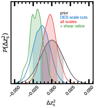
Photo-z distributions: An advantage of using shear ratios is that they provide information on the redshift distribution of background galaxies. Notably, we find that small scales provide a similar level of information on photometric redshifts. It is thus interesting to compare their constraints since including shear ratios or not does affect the inferred $S_{8}$ value. We show, as an example, the posterior of $\Delta z_{\rm s}^{2}$ in Fig. 9 (see Appendix F for other redshift bins). This is the photo-z parameter that differs the most between our analysis and that of DES with shear ratios.

Figure 10: Impact of the different modelling choices to explain the different fiducial cosmological constraints obtained by the DES Collaboration (DES TATT + SR, Secco et al., 2022; Amon et al., 2022) and this work (BACCOemu NLA BCM). We show the $1\sigma$ credible level of $S_{8}$ and $\Omega_{\rm m}$ (solid lines) and maximum posteriors (stars), obtained by the DES Collaboration with the CosmoSIS pipeline and different choices regarding the intrinsic alignment model and the use of shear ratios (black, brown, red, according to the legend). Analogously, we show also our results, obtained with the BACCO pipeline using HALOFIT (orange), or BACCOemu without and with baryons (green and blue, respectively).

Firstly, we see that including the small scales provides a constraining power on $\Delta z_{\rm s}^{2}$ competitive with that of shear ratios, even after marginalisation over baryons. Specifically, in our fiducial analysis we obtain $\sigma[\Delta z_{\rm s}^{2}]\sim 0.012$ when applying DES scale cuts, and $\sim 0.01$ when including small scales – a comparable precision to that by including shear ratios $\sim 0.009$. Of course, our approach has the advantage of not relying on the modelling of the galaxy-galaxy lensing, and thus galaxy bias, lenses redshift distributions, etc.

Moreover, we note that our posterior on $\Delta z_{\rm s}^{2}$ is in good agreement with the Gaussian prior and with the analysis with DES scale cuts. Instead, when using shear ratios, the data prefer a shift in the mean photo-z of $\sim 0.0025$. Given the sensitivity of the shear signal to the sources’ redshift distributions, these might cause part of the small shift in the cosmological constraints observed when comparing results with and without shear ratios. The information contained in the small scales of the cosmic shear is not in alarming tension with the one contained in the small scales of shear ratios. However, as the precision of WL surveys increases, this comparison can provide a good sanity check to highlight possible shortcomings of the modelling of cosmic shear and galaxy-galaxy lensing.

Nonlinear modelling: Another difference is that we employ a more precise model for the nonlinear matter power spectrum, especially in the case of massive neutrinos. We show in Appendix A the difference in our cosmology constraints obtained when using our non-linear emulator or HALOFIT used by the DES Collaboration. By using BACCOemu, the $S_{8}$ constraints are shifted by $0.4\sigma$ toward high values when applying DES scale cuts, and up to $0.5$ when considering all angular scales. The slightly different choice for the $M_{\nu}$ prior has a comparatively small effect of $0.1\sigma$.

Baryonic modelling and pipeline: Finally, we note an extra $0.2\sigma$ shift caused by the marginalisation over baryons when applying DES scale cuts. We should also consider a $0.1\sigma$ shift given by the pipeline implementations in BACCO and CosmoSIS.

To summarise, we find that the fiducial modelling of intrinsic alignment and non-linearities cause the largest shift in $S_{8}$. Notably, most of the effects listed here shift the $S_{8}$ posterior toward higher values. Thus, as shown in Fig.10, also smaller effects (with DES scale cuts) e.g. the baryon marginalisation and the addition of shear ratios, other than the difference in $M_{\nu}$ prior, sum up to make the final $1.4\sigma$ discrepancy that we report.

5.3 Comparison with other datasets

When assuming $\Lambda$CDM, several authors have claimed that LSS observations prefer statistically lower values of $S_{8}$ compared to temperature and polarization fluctuations measured by Planck (Planck Collaboration et al., 2018). For instance, by using only BOSS data and exploiting the full shape of the galaxy power spectrum and bispectrum, Philcox & Ivanov (2022) inferred $S_{8}=0.751\pm 0.039$ – a figure that is in agreement with lensing measurements and lower than Planck. Nunes & Vagnozzi (2021) used a compilation of growth rates from the redshift space distortions (RSD) measured in different surveys, combined with Baryonic Acoustic Oscillations (BAO) and type Ia supernovae, and found $S_{8}=0.762^{+0.030}_{-0.025}$.

Regarding weak lensing data, Secco et al. (2022); Amon et al. (2022) found that DES Y3 cosmic shear is at $2.3\sigma$ tension with Planck, according to the so-called Bayesian Suspiciousness (Handley & Lemos, 2019), where the prior volume effects are removed from the Bayes ratios. When projected to the $S_{8}$ parameters, they found $S_{8}=0.759^{+0.025}_{-0.023}$ while Planck data suggests $S_{8}=0.826^{+0.019}_{-0.016}$. Adding galaxy-galaxy lensing and galaxy clustering (3x2pt analysis) the Suspiciousness lowered down to $0.7\sigma$.

Similarly, with the cosmic shear analysis of the Kilo Degree Survey (KiDS), Asgari et al. (2021) measured $S_{8}=0.759^{+0.024}_{.0.021}$ and reported a $3\sigma$ tension in the $S_{8}$ posterior. Combining the KiDS cosmic shear analysis with the redshift-space galaxy clustering from the Baryon Oscillation Spectroscopic Survey (BOSS, Alam et al., 2015) and the 2-degree Field Lensing Survey (2dFLenS, Blake et al., 2016), Heymans et al. (2021) got $S_{8}=0.766^{+0.020}_{-0.014}$, and claimed a tension with Planck between $2\sigma$ and $3\sigma$.

Recently, the Subaru Hyper Supreme-Cam (HSC) Collaboration published the cosmic shear analysis after the third year of data collection, reporting $S_{8}=0.769^{+0.031}_{-0.034}$ with correlation functions (Li et al., 2023), and $S_{8}=0.776^{+0.032}_{-0.033}$ with power spectra (Dalal et al., 2023).

Our fiducial constraint on $S_{8}$ is systematically higher but in broad agreement with results from the shear-only analyses of these surveys. Our preferred value is approximately $1.5\sigma$ higher than that of KIDS-1000, $1.4\sigma$ higher than in DES Y3, and $0.8\sigma$ above HSC Y3 (analysis with correlation functions). It is, however, unclear how much of this tension would be reduced by homogenising analysis choices and the improvements we adopt in our pipeline, given the different scales and redshifts probed in the analyses. At the small scales, KiDS-1000 stops at 0.5 arcmins in $xi_{+}$ and 4 arcmins in $xi_{-}$, whereas HSC Y3 to $7.1$ arcmins in $\xi_{+}$ and 31.2 arcmins in $\xi_{-}$. Both the surveys model the baryonic suppression with HMcode (Mead et al., 2015).

Using more refined baryonic modelling, the BCM emulator described in Giri & Schneider (2021), Schneider et al. (2022) analysed the cosmic shear measured by KiDS-1000 using external data from X-ray and kinetic Sunyaev-Zel’dovich (kSZ). In agreement with our results, they found that baryons reduce the tension with Planck, from $3.8\sigma$ to $2.6\sigma$ in KiDS. They notice that KiDS-1000 data alone are not enough to constrain baryonic physics (whereas we find that DES Y3, arguably due to the larger sky area, can constrain the most important parameter, $M_{\rm c}$). By adding X-ray and kinetic Sunyaev-Zel’dovich (SZ) data, they were able to constrain 3 out of 7 baryonic parameters, and measure a mild-strong feedback broadly in agreement with that measured with DES Y3. Overall, they find a similar impact of baryons on cosmology to what we find when analysing all the angular scales of DES Y3, a shift in $S_{8}$ of about $1\sigma$ towards higher $S_{8}$.

Using HMcode (Mead et al., 2020b) as a model for baryons, Tröster et al. (2022) combined the cosmic shear from KiDS-1000 with the cross-correlation between shear and thermal SZ (tSZ), measured by Planck and the Atacama Cosmology Telescope (ACT) (Mallaby-Kay et al., 2021). They find an improvement on the $S_{8}$ constraint of $40\%$ in the joint analysis but did not reduce the S8 tension: they infer $S_{8}=0.751^{+0.020}_{-0.017}$, at $3.4\sigma$ from Planck (see also a similar analysis by Robertson et al. (2021) cross-correlating KiDS with Planck/ACT CMB lensing. However, since HMcode has been explicitly calibrated to reproduce the BAHAMAS hydrodynamical simulations, it is not clear whether these results would hold with more flexible baryonic modelling such as that we propose here.

Interestingly, a very recent analysis of the CMB lensing from ACT DR6, in combination with BAO data, reports $S_{8}=0.849\pm 0.028$ (Madhavacheril et al., 2023; Qu et al., 2023), in perfect agreement with the inference from Planck CMB anisotropies.

A different way to improve the accuracy of current constraints is to take advantage of the fact that, at the moment, LSS surveys are largely independent of each other. Combining 6 different cosmic shear, galaxy clustering, and CMB lensing surveys, García-García et al. (2021) placed a tight constraint $S_{8}=778^{+0.009}_{-0.009}$, $3.4\sigma$ in tension with Planck. Unfortunately, precise non-linearities and baryons were not included in this analysis. Additionally, the modelling inevitably requires several assumptions regarding the way in which galaxies trace the underlying matter field.

Finally, as we have discussed in the previous section, our analysis pipeline and choices deliver constraints that are somewhat in tension with those of the official DES Collaboration. Thus, it would be interesting in the future to re-analise jointly the data from KiDS and HSC including small-scale information and the advances we have described in this paper. Furthermore, as these WL surveys provide measurements that are at different redshifts, they could be combined to further constrain the time evolution of baryonic processes.

Similarly, it is important to study more in-depth the role of the intrinsic alignment models and photo-z systematic errors. Finally, to robustly combine WL with clustering data, it will be essential to carefully consider the accuracy of current models for galaxy biasing. For instance, correlations between galaxy number and halo properties, baryons, and assembly bias all affect galaxy clustering and galaxy-galaxy lensing in different manners (see e.g. Chaves-Montero et al., 2023; Contreras et al., 2023), but are commonly neglected in mock catalogues used to validate lensing pipelines. We plan to address all these issues in the future.

6 Conclusions

In this paper we have analysed the cosmic shear correlation functions measured in DES Y3, exploiting for the first time all the angular scales measured. We have implemented a new fast pipeline to predict the cosmic shear correlation functions, and employed the neural network emulators of BACCOemu to accurately predict the matter power spectrum with non-linearities and baryonic effects. Our main findings are the following:

• We find additional information at small scales. Constraints on $S_{8}$ are tighter by $30\%$ when ignoring astrophysical processes, and still $10\%$ ($15\%$) tighter when marginalising over 7 (1) baryonic parameters. These numbers are specific to DES and we expect the gains to be larger in upcoming surveys.

• The $S_{8}$ posterior shifts by $\approx 0.5\sigma$ towards lower values when removing DES scale cuts and not modelling baryonic effects. The cosmological inference is instead robust against scale cuts when modelling baryons with a baryonification algorithm (Fig. 3);

• We constrain baryonic feedback via the BCM parameter $M_{\rm c}$. We obtain $\log M_{\rm c}[h^{-1}{\rm M_{\odot}}]=14.38^{+0.60}_{-0.56}$ which means haloes with mass $M_{200,c}=10^{14}h^{-1}{\rm M_{\odot}}$ have lost half of their gas reservoir (Fig. 4).

• We find a correlation between $S_{8}$ and $M_{\rm c}$, so that stronger baryonic effects correspond to higher $S_{8}$. In light of the $S_{8}$ tension, this means that stronger baryonic feedback increases the agreement between DES Y3 and Planck (Fig. 6).

• We infer $S_{8}=0.799^{+0.023}_{-0.015}$ and $\Omega_{\rm m}=0.252^{+0.066}_{-0.030}$ when including the entire range of scales in DES and conservatively marginalising over 7 free baryonic parameters. This value $S_{8}$ is $0.9\sigma$ lower than that preferred by Planck TT+TE+EE+lowE data (Fig. 7).

• Our inferred value of $S_{8}$ differs from that inferred in the official DES analysis by $1.4\sigma$ (Fig. 10). This is a significant difference since both analyses employ very similar datasets. We attribute the discrepancy to five factors: i) the modelling of intrinsic alignments; ii) the computation of the nonlinear power spectrum; iii) the modelling of baryons; iv) the employment of shear ratios by the DES Collaboration; v) minor difference between the pipeline and priors used.

We can conclude that, with current data, the modelling details impact significantly the parameter inference, and therefore the assessment of tensions between different datasets. Improving the modelling, as well as explicitly taking into account the theoretical uncertainties in the analysis, appears to be a key step to delivering robust cosmological constraints.

We have shown that we can accurately model the cosmic shear of DES Y3, down to the smallest scales available. At these scales, cosmology and astrophysical processes are tightly intertwined, and disentangling them is not an easy task.

In the future, we plan to do it by consistently joining different datasets. Specifically, we will perform a 3x2pt analysis, modelling also galaxy-galaxy lensing and galaxy clustering to very small scales, by exploiting non-linear bias emulators included in BACCOemu (Zennaro et al., 2021; Pellejero Ibañez et al., 2022; Pellejero-Ibanez et al., 2022). To inform the baryonic model, we plan to use X-ray, thermal & kinetic Sunyaev-Zel’dovich datasets, and their cross-correlations when possible. Such an analysis will be of particular importance in light of the upcoming surveys, such as Euclid and LSST, where the solidity of our modelling framework will be stress-tested in an unprecedented way.

Appendix A Modelling of non-linearities

Figure 11: $1\sigma$ and $2\sigma$ credible interval on $S_{8}$ and $\Omega_{\rm m}$ when modelling the matter power spectrum with HALOFIT (black) or BACCOemu (red). All the angular scales are used, not considering baryonic processes.

The DES Collaboration employs HALOFIT (Takahashi et al., 2012) to predict the nonlinear matter power spectrum (e.g. Secco et al., 2022; Amon et al., 2022). HALOFIT has a nominal accuracy of $10\%$ at $k=10\,h\,{\rm Mpc}^{-1}$ (Takahashi et al., 2012). Krause et al. (2021) have shown that accuracy is enough to model the shear signal over the scales relevant for DES Y3, i.e. it causes a shift $<0.3\sigma$ compared to the EuclidEmulator and CosmoEmu emulators (Euclid Collaboration et al., 2020; Heitmann et al., 2014).

Generally, the accuracy of HALOFIT, as well as HMcode, BACCOemu, and other emulators, has been tested only over a relatively small cosmological space with respect to the prior used in DES analysis or even compared to the $\sim 2-3\sigma$ regions of the posteriors. This could cause bias in cosmological parameters as the error could be significantly larger in some regions of the parameter space, for instance, for very massive neutrinos.

To test the performance of HALOFIT in a larger cosmological space, we have carried out a suite of 20 $N-$body simulations with cosmological parameters randomly distributed over the prior space. These simulations have a mass resolution so that the power spectrum is converged at a few per cent level at $z=0$ and $k=10h\,{\rm Mpc}^{-1}$. We find that HALOFIT performs remarkably well – considering that it was fitted to only 16 $N-$body simulations – achieving a precision of around $20\%$. This, however, could still introduce significant biases in our cosmological constraints.

Building emulators over large cosmological space volumes is very challenging. This would in principle require a large number of high-resolution simulations. Alternatively, here we exploit the cosmology scaling of Angulo & White (2010); Angulo et al. (2021). Therefore, we build an updated version of BACCOemu by employing a suite of 35 $N-$body simulations run with various cosmologies. These simulations were then scaled to more than 1000 cosmological parameter sets and 10 redshifts. We then train a neural network that quickly predicts the nonlinear power spectrum. We estimate that our emulator reaches a precision of about $5-10\%$ to $k=10\,h\,{\rm Mpc}^{-1}$. We refer to Zennaro et al. (in prep.) for all the details.

We now check the differences in the cosmology inference using either HALOFIT or BACCOemu, when modelling the DES Y3 shear correlation functions down to angles $\theta=2.5\,{\rm arcmins}$. For this test, we use an NLA model and do not include baryonic processes to isolate the effects of the non-linear matter power spectrum. Fig. 11 shows how the $1\sigma$ and $2\sigma$ credible levels of $S_{8}$ obtained with BACCOemu are systematically higher with respect to HALOFIT by almost $0.5\sigma$. When applying DES scale cuts, the difference is slightly smaller, about $0.4\sigma$, due to a smaller amount of non-linearities in the data vector. Thus, we find a larger bias given by non-linearities with respect to Krause et al. (2021), arguably because of the larger cosmological parameters space used here, where the accuracy of HALOFIT is lower.

Appendix B Comparison against hydrodynamical simulations

Figure 12: $1\sigma$ and $2\sigma$ credible levels on $S_{8}$ and $\Omega_{\rm m}$ obtained by assuming the baryonic feedback measured in BAHAMAS (black), and using the BCM with the best-fitting parameters to the matter power spectrum at $z=0$ of BAHAMAS (red).

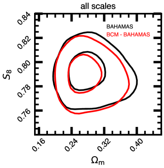
The baryonification emulator in BACCOemu has been extensively tested against several hydrodynamical simulations (Aricò et al., 2021b; Chen et al., 2023). Here, we further test the ability of the emulator to mimic the impact of the baryonic processes as predicted by a complex hydrodynamical simulation. To do so, we take the suppression in the matter power spectrum measured in BAHAMAS (McCarthy et al., 2017; McCarthy et al., 2018), at $z\in[0.,3.]$ and $k\in[10^{-2},5\times 10^{2}]h\,{\rm Mpc}^{-1}$, and use it as a fiducial baryonic suppression for the cosmology inference in the analysis of the cosmic shear measured by DES Y3. We compare it to the results that we obtain when employing the BCM, fixing the free parameters to the best-fitting values to the matter power spectrum of BAHAMAS at $z=0$. The best-fitting parameters, obtained by Aricò et al. (2021b), are $\log{M_{\rm c}}=13.62[\log(h^{-1}{\rm M_{\odot}})]$, $\log{\eta_{b}}=-0.33$, $\log{\beta_{b}}=-0.28$, $\log M_{z0,\rm cen}=10.21[\log(h^{-1}{\rm M_{\odot}})]$, $\log{\theta_{\rm inn}}=-0.62$, $\log{\theta_{\rm out}}=0.12$, $\log{M_{\rm inn}}=9.95[\log(h^{-1}{\rm M_{\odot}})]$.

We show the comparison between the two posteriors in the $S_{8}$-$\Omega_{\rm m}$ plane in Fig. 12. The cosmological constraints are in very good agreement, highlighting the remarkable flexibility and accuracy of the BCM emulator, and assessing its adequacy to study DES Y3 data. In particular, this shows the negligible impact of the relatively restricted regime of validity of the emulator ($z\in[0.,2.5]$ and $k\in[10^{-2},10\,h\,{\rm Mpc}^{-1}$]), and of the assumption of no redshift evolution of the baryonification parameters.

Appendix C Cosmological parameters

Figure 13: Posteriors of the cosmological parameters, obtained analysing all the angular scales of DES Y3 cosmic shear with our fiducial model (black). For comparison, we over plot the $1\sigma$ and $2\sigma$ credible levels obtained with DES scale cuts (red).

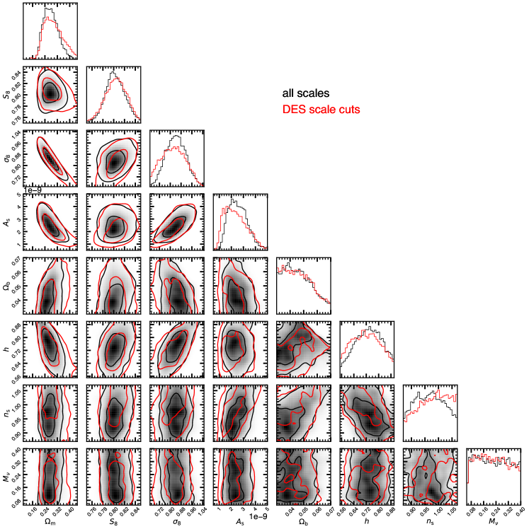
We present in Fig. 13 the posteriors of all the free cosmological parameters in our analyses, when applying DES scale cuts and when analysing all the scales. The main gain in constraining power when analysing the small scales is in $\Omega_{\rm m}$, and $S_{8}$ or alternatively $\sigma_{8}$. We get somewhat better constraints also in the Hubble parameter. Specifically, when analysing the full data vector, we constrain the normalisation of the primordial linear matter power spectrum $A_{\rm s}=\left(23.1^{+8.9}_{-7.0}\right)\times 10^{-10}$ and the amplitude of the linear matter density fluctuations $\sigma_{8}=0.843^{+0.072}_{-0.081}$. We also weakly constrain the dimensionless Hubble constant $h=0.742^{+0.096}_{-0.098}$, and the tilt of the primordial matter power spectrum, $n_{\rm s}=0.971^{+0.057}_{-0.071}$. The baryonic density remains unconstrained (although high values of $\Omega_{\rm b}$ are slightly disfavoured), as well as the sum of neutrino masses $M_{\nu}$.

Model	$S_{8}$		$\Omega_{\rm m}$
This work	DES scale cuts	all scales	DES scale cuts	all scales
NLA BCM7 (fiducial)	$0.804^{+0.021}_{-0.021}$	$0.802^{+0.020}_{-0.018}$	$0.291^{+0.074}_{-0.055}$	$0.275^{+0.053}_{-0.045}$
NLA GrO	$0.800^{+0.019}_{-0.021}$	$0.787^{+0.014}_{-0.015}$	$0.287^{+0.064}_{-0.052}$	$0.270^{+0.063}_{-0.040}$
NLA BCM1	$0.803^{+0.019}_{-0.019}$	$0.798^{+0.016}_{-0.018}$	$0.285^{+0.067}_{-0.053}$	$0.274^{+0.060}_{-0.045}$
NLA BCM-extreme	$0.841^{+0.025}_{-0.027}$	$0.829^{+0.023}_{-0.022}$	$0.286^{+0.069}_{-0.053}$	$0.300^{+0.060}_{-0.054}$
TATT BCM7	$0.792^{+0.024}_{-0.026}$	$0.781^{+0.028}_{-0.037}$	$0.292^{+0.068}_{-0.052}$	$0.249^{+0.057}_{-0.039}$
TATT GrO	$0.788^{+0.024}_{-0.027}$	$0.756^{+0.025}_{-0.027}$	$0.277^{+0.062}_{-0.047}$	$0.270^{+0.061}_{-0.042}$
TATT BCM1	$0.791^{+0.024}_{-0.029}$	$0.780^{+0.025}_{-0.037}$	$0.276^{+0.068}_{-0.050}$	$0.250^{+0.050}_{-0.035}$
TATT BCM-extreme	$0.825^{+0.030}_{-0.031}$	$0.815^{+0.029}_{-0.037}$	$0.283^{+0.072}_{-0.054}$	$0.258^{+0.058}_{-0.039}$
DES Collaboration
DES NLA	$0.784^{+0.022}_{-0.023}$	-	$0.310^{+0.069}_{-0.057}$	-
DES NLA + SR	$0.773^{+0.020}_{-0.020}$	-	$0.289^{+0.054}_{-0.046}$	-
DES TATT	$0.759^{+0.032}_{-0.038}$	-	$0.293^{+0.064}_{-0.052}$	-
DES TATT + SR (fiducial)	$0.759^{+0.023}_{-0.024}$	-	$0.285^{+0.058}_{-0.048}$	-

Table 4: Constraints (median of the 1D marginalised posteriors and respective 34th percentiles) on $S_{8}$ and $\Omega_{\rm m}$ obtained applying DES scale cuts and using all the angular scales. We explore different models, with NLA or TATT intrinsic alignment, gravity-only, or applying a baryonification with 1 or 7 free parameters (BCM1, BCM7, respectively). We also include a model with an extreme implementation of AGN feedback. We report for comparison the constraints we get analysing the DES Collaboration chains, with and without shear ratios (SR).

We also report here Tab. 4, where we quote the median of the 1D marginalised posteriors on $S_{8}$ and $\Omega_{\rm m}$ and their respective 34th percentiles (as opposed to the maximum posterior of Tab. 3). We report for comparison the values we get when analysing the DES Collaboration chains (Secco et al., 2022; Amon et al., 2022), as in the official DES papers they typically report the mean values instead.

Appendix D Baryonic parameters

Figure 14: Posteriors of the baryonic parameters, obtained analysing all the angular scales of DES Y3 cosmic shear with our fiducial model.

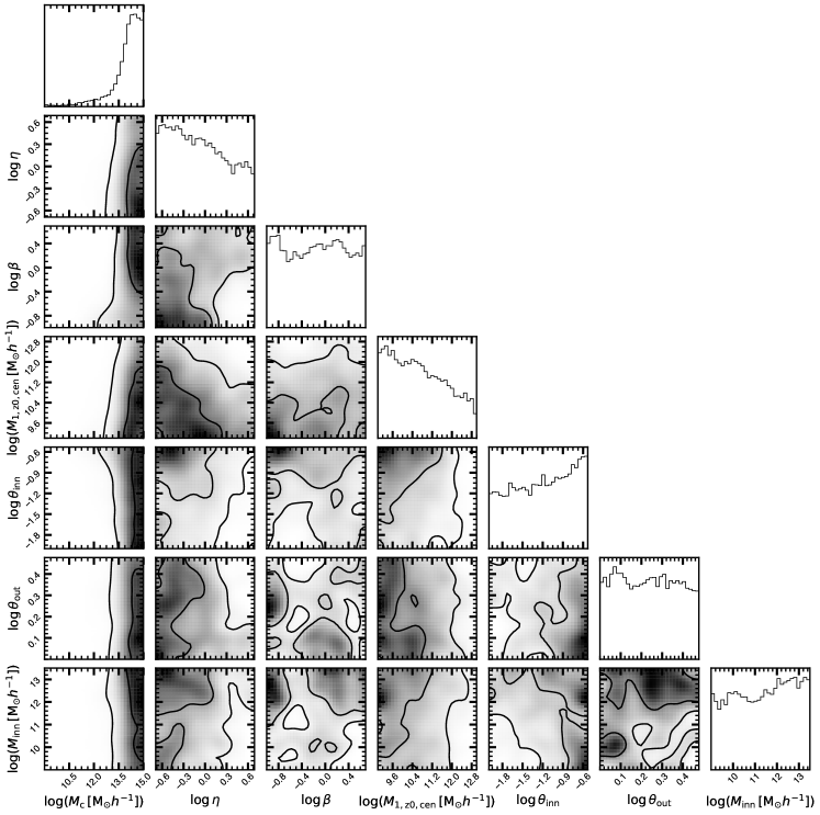
In the main text we have reported the posterior of $M_{\rm c}$, the only baryonic parameter strongly constrained by the cosmic shear of DES Y3. Here we report for completeness the posteriors of all the 7 baryonic parameters available in BACCOemu.

The parameters are: $\eta$, which regulate the baryonic feedback range; $\beta$, the slope of the gas fraction - halo mass; the gas density shape ($\theta_{\rm inn}$,$\theta_{\rm out}$,$M_{\rm inn}$); and $M_{z0,\rm cen}$, the galaxy-halo mass relation. We show in Fig. 14 their posteriors. $M_{\rm c}$ is the only parameter significantly constrained: we obtained $\log M_{\rm c}=14.38^{+0.60}_{-0.56}\,[\log(h^{-1}{\rm M_{\odot}})]$. The constraints are robust to the intrinsic alignment model assumed.

Appendix E Tidal-Alignment & Tidal-Torque

Figure 15: Posteriors of $S_{8}$ of DES Y3 cosmic shear, when employing as intrinsic alignment model NLA (red) or TATT (blue), compared to Planck TT+TE+EE+lowE. To model DES Y3 cosmic shear we have considered a 7-free parameters baryonification. We show with dotted lines the posteriors that we obtain when imposing a physically-motivated prior on the intrinsic alignment amplitude $a_{1}\in[0,5]$.

Figure 16: Posteriors of TATT parameters when analysing all the angular scales of DES Y3 cosmic shear with our fiducial model (black). For comparison, we overplot the $1\sigma$ and $2\sigma$ credible levels obtained with DES scale cuts (red).

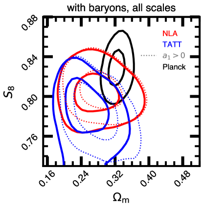
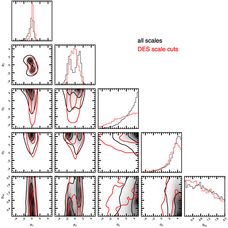
The Tidal-Alignment & Tidal-Torque (TATT) model is inspired by perturbation theory and aims to predict the intrinsic alignment of galaxies by considering a perturbative expansion of the cosmic density and tidal fields (Blazek et al., 2019). There are three terms considered: a linear term (tidal alignment), a quadratic term (tidal torque), and a cross term, with a total of 5 free parameters $a_{1}$, $\eta_{1}$, $a_{2}$, $\eta_{2}$, $b_{\rm TA}$. We have reported the respective equations in §3.2.

It is not clear on which scales the NLA and TATT are valid, since the theoretical limits given by linear and perturbation theory are practically overcome by using a full non-linear power spectrum. Generally, this is dependent on the galaxy sample analysed, since red galaxies are expected to have higher tidal alignment amplitudes ( $a_{1}\in\left[3,5\right]$) than blue galaxies ($a_{1}\in\left[0,1\right]$ ) (Samuroff et al., 2019, 2022).

The cosmic shear analysis made by the DES Collaboration on year 3 data has highlighted a low amplitude of intrinsic alignment $a_{1}=-0.47^{+0.30}_{-0.52}$ and $a_{2}=1.02^{+1.61}_{-0.55}$, much lower than the cosmological signal (Secco et al., 2022; Amon et al., 2022). Indeed, a model without an intrinsic alignment is marginally preferred with respect to NLA and TATT by Bayesian evidence. Therefore, Secco et al. (2022); Amon et al. (2022) conclude a posteriori that both NLA and TATT are suited for the analysis of DES Y3 data.

Here we are employing smaller scales than in the analysis of Secco et al. (2022); Amon et al. (2022), thus we reassess the impact of scale cuts on the intrinsic alignment parameters after marginalising over 7 baryonic parameters. We have checked that the marginalisation only slightly degrades the TATT parameters constraints, without shifting them in any particular direction.

We show the posteriors of the TATT parameters in Fig. 16, with and without DES scale cuts (black and red lines, respectively). With scale cuts, we obtain $a_{1}=0.13^{+0.46}_{-0.26}$ and $a_{2}=0.00^{+0.48}_{-1.42}$, whereas we obtain $a_{1}=-0.01^{+0.49}_{-0.63}$ and a fully bimodal $a_{2}$ when using all the scales. The amplitudes we find are consistent with zero in both cases. As noticed in Secco et al. (2022); Amon et al. (2022), $a_{2}$ presents a multi-modal posterior. In contrast to Secco et al. (2022); Amon et al. (2022), which reports that adding more data points at small scales (their $\Lambda$CDM-optimised case) the multimodality was alleviated, we find that adding small scales the multi-modality is exacerbated. According to Amon et al. (2022), this multi-modality is given by internal degeneracies in the TATT model and it can degrade and shift the posterior on $S_{8}$.

In Fig. 15 we show the posterior projected onto the $S_{8}$ - $\Omega_{\rm m}$ plane when assuming NLA and TATT, and comparing it to Planck. Employing TATT we get $S_{8}=0.788^{+0.027}_{-0.035}$, a looser constraint with respect to NLA. We see that the posterior shifts also lower $S_{8}$ and $\Omega_{\rm m}$, at $\approx 2\sigma$ from Planck. This could be an effect of the degeneracy between $a_{1}$ and $a_{2}$ discussed above. As noted by Secco et al. (2022); Amon et al. (2022), one would expect the intrinsic alignment amplitude $a_{1}\geq 0$ in absence of systematics. Therefore, we impose $a_{1}\geq 0$ as a prior, and obtain the dotted contours in Fig. 15. With NLA, this new prior slightly shifts ($0.1\sigma$) the $S_{8}$ contours towards Planck, whereas with TATT the largest effect is a shift of $0.4\%$ in $\Omega_{\rm m}$.

Appendix F Shear bias & Photo-z uncertainties

Figure 17: Priors (gray dotted lines) and posteriors of the shear biases $m^{\rm i}$ and photo-z uncertainties $\Delta z_{\rm s}^{i}$, obtained with our fiducial for baryons and intrinsic alignment (BCM & NLA, respectively). We display the cases when applying DES scale cuts (black) and using all angular scales (red), and compare against the results obtained by the DES Collaboration using NLA with the addition of the shear ratios likelihood (blue, Secco et al., 2022; Amon et al., 2022).

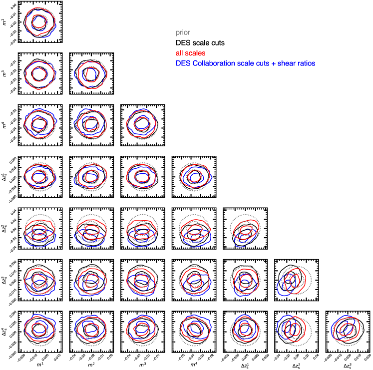
We display in Fig. 17 the parameter posteriors of the shear biases $m^{\rm i}$, that take accounts of galaxy shapes miscalibration and blending, and the photo-z uncertainties $\Delta z_{\rm s}^{i}$, that is the shift of the source redshift distribution in the $i$ bin. We show the posteriors obtained with and without scale cuts, using NLA and marginalising over 7 free baryonic parameters. We compare against the respective informative Gaussian priors, and additionally to the posteriors obtained by the DES Collaboration adding the likelihood of the lensing shear ratios. Such ratios are shown to be particularly sensitive to the redshift distribution of the source galaxies (Sánchez et al., 2022; Amon et al., 2022).

The posteriors of the shear biases are all in good agreement, in some cases, e.g. $m^{4}$, analysing the small scales gives an improvement in the constraints similar to the addition of the shear ratios.

Also the $\Delta z_{\rm s}^{i}$ posteriors are in good agreement with the priors. We note how the constraints obtained with shear ratios are generally tighter with respect to the ones with scale cuts, and in agreement with our full-scale analysis. In some cases, notably $\Delta z_{\rm s}^{2}$ and $\Delta z_{\rm s}^{3}$, the results we obtain analysing the full data vector and the results obtained by the DES Collaboration using large scales and shear ratios are slightly in tension, being our constraints more in agreement with the priors.

References

- Abbott et al. (2022) Abbott T. M. C., et al., 2022, Phys. Rev. D, 105, 023520
- Alam et al. (2015) Alam S., et al., 2015, ApJS, 219, 12
- Amon & Efstathiou (2022) Amon A., Efstathiou G., 2022, MNRAS, 516, 5355
- Amon et al. (2022) Amon A., et al., 2022, Phys. Rev. D, 105, 023514
- Angulo & Hilbert (2015) Angulo R. E., Hilbert S., 2015, MNRAS, 448, 364
- Angulo & White (2010) Angulo R. E., White S. D. M., 2010, MNRAS, 405, 143
- Angulo et al. (2021) Angulo R. E., Zennaro M., Contreras S., Aricò G., Pellejero-Ibañez M., Stücker J., 2021, MNRAS, 507, 5869
- Aricò et al. (2020) Aricò G., Angulo R. E., Hernández-Monteagudo C., Contreras S., Zennaro M., Pellejero-Ibañez M., Rosas-Guevara Y., 2020, MNRAS, 495, 4800
- Aricò et al. (2021a) Aricò G., Angulo R. E., Hernández-Monteagudo C., Contreras S., Zennaro M., 2021a, MNRAS, 503, 3596
- Aricò et al. (2021b) Aricò G., Angulo R. E., Contreras S., Ondaro-Mallea L., Pellejero-Ibañez M., Zennaro M., 2021b, MNRAS, 506, 4070
- Aricò et al. (2022) Aricò G., Angulo R. E., Zennaro M., 2022, Open Research Europe, 499, arXiv:2104.14568
- Arnaud et al. (2007) Arnaud M., Pointecouteau E., Pratt G. W., 2007, A&A, 474, L37
- Asgari et al. (2021) Asgari M., et al., 2021, A&A, 645, A104
- Beringer et al. (2012) Beringer J., et al., 2012, Phys. Rev. D, 86, 010001
- Blake et al. (2016) Blake C., et al., 2016, MNRAS, 462, 4240
- Blazek et al. (2019) Blazek J. A., MacCrann N., Troxel M. A., Fang X., 2019, Phys. Rev. D, 100, 103506
- Bridle & King (2007) Bridle S., King L., 2007, New Journal of Physics, 9, 444
- Bucko et al. (2022) Bucko J., Giri S. K., Schneider A., 2022, arXiv e-prints, p. arXiv:2211.14334
- Chaves-Montero et al. (2023) Chaves-Montero J., Angulo R. E., Contreras S., 2023, MNRAS,
- Chen et al. (2021) Chen A., et al., 2021, Phys. Rev. D, 103, 123528
- Chen et al. (2023) Chen A., et al., 2023, MNRAS, 518, 5340
- Chisari et al. (2018) Chisari N. E., et al., 2018, MNRAS, 480, 3962
- Chisari et al. (2019) Chisari N. E., et al., 2019, ApJS, 242, 2
- Contreras et al. (2020) Contreras S., Angulo R. E., Zennaro M., Aricò G., Pellejero-Ibañez M., 2020, MNRAS, 499, 4905
- Contreras et al. (2023) Contreras S., Angulo R. E., Chaves-Montero J., White S. D. M., Aricò G., 2023, MNRAS, 520, 489
- Crain et al. (2015) Crain R. A., et al., 2015, MNRAS, 450, 1937
- Crittenden et al. (2002) Crittenden R. G., Natarajan P., Pen U.-L., Theuns T., 2002, ApJ, 568, 20
- DESI Collaboration et al. (2016) DESI Collaboration et al., 2016, arXiv e-prints, p. arXiv:1611.00036
- Dalal et al. (2023) Dalal R., et al., 2023, arXiv e-prints, p. arXiv:2304.00701
- Dark Energy Survey Collaboration et al. (2016) Dark Energy Survey Collaboration et al., 2016, MNRAS, 460, 1270
- Debackere et al. (2019) Debackere S. N. B., Schaye J., Hoekstra H., 2019, arXiv e-prints,
- Eifler et al. (2015) Eifler T., Krause E., Dodelson S., Zentner A. R., Hearin A. P., Gnedin N. Y., 2015, MNRAS, 454, 2451
- Euclid Collaboration et al. (2020) Euclid Collaboration et al., 2020, arXiv e-prints, p. arXiv:2010.11288
- Fang et al. (2017) Fang X., Blazek J. A., McEwen J. E., Hirata C. M., 2017, J. Cosmology Astropart. Phys., 2017, 030
- Fedeli (2014) Fedeli C., 2014, J. Cosmology Astropart. Phys., 4, 028
- Flaugher et al. (2015) Flaugher B., et al., 2015, AJ, 150, 150
- Foreman-Mackey (2016) Foreman-Mackey D., 2016, The Journal of Open Source Software, 1, 24
- Friedrich et al. (2021) Friedrich O., et al., 2021, MNRAS, 508, 3125
- García-García et al. (2021) García-García C., Ruiz-Zapatero J., Alonso D., Bellini E., Ferreira P. G., Mueller E.-M., Nicola A., Ruiz-Lapuente P., 2021, J. Cosmology Astropart. Phys., 2021, 030
- Gatti et al. (2021) Gatti M., et al., 2021, MNRAS, 504, 4312
- Giodini et al. (2009) Giodini S., et al., 2009, ApJ, 703, 982
- Giri & Schneider (2021) Giri S. K., Schneider A., 2021, J. Cosmology Astropart. Phys., 2021, 046
- Gonzalez et al. (2013) Gonzalez A. H., Sivanandam S., Zabludoff A. I., Zaritsky D., 2013, ApJ, 778, 14
- Gu et al. (2023) Gu S., Dor M.-A., van Waerbeke L., Asgari M., Mead A., Tröster T., Yan Z., 2023, arXiv e-prints, p. arXiv:2302.00780
- Handley (2019) Handley W., 2019, Journal of Open Source Software, 4, 1414
- Handley & Lemos (2019) Handley W., Lemos P., 2019, Phys. Rev. D, 100, 043504
- Handley et al. (2015) Handley W. J., Hobson M. P., Lasenby A. N., 2015, MNRAS, 450, L61
- Harnois-Déraps et al. (2015) Harnois-Déraps J., van Waerbeke L., Viola M., Heymans C., 2015, MNRAS, 450, 1212
- Harris et al. (2020) Harris C. R., et al., 2020, Nature, 585, 357
- Heisenberg et al. (2023) Heisenberg L., Villarrubia-Rojo H., Zosso J., 2023, Physics of the Dark Universe, 39, 101163
- Heitmann et al. (2014) Heitmann K., Lawrence E., Kwan J., Habib S., Higdon D., 2014, ApJ, 780, 111
- Heymans et al. (2021) Heymans C., et al., 2021, A&A, 646, A140
- Hikage et al. (2019) Hikage C., et al., 2019, PASJ, 71, 43
- Hinton (2016) Hinton S. R., 2016, The Journal of Open Source Software, 1, 00045
- Hirata & Seljak (2004) Hirata C. M., Seljak U., 2004, Phys. Rev. D, 70, 063526
- Huang et al. (2019) Huang H.-J., Eifler T., Mandelbaum R., Dodelson S., 2019, MNRAS, 488, 1652
- Hunter (2007) Hunter J. D., 2007, Computing in Science & Engineering, 9, 90
- Ivezić et al. (2019) Ivezić Ž., et al., 2019, ApJ, 873, 111
- Jeffreys (1935) Jeffreys H., 1935, Mathematical Proceedings of the Cambridge Philosophical Society, 31, 203–222
- Kitching et al. (2017) Kitching T. D., Alsing J., Heavens A. F., Jimenez R., McEwen J. D., Verde L., 2017, MNRAS, 469, 2737
- Krause et al. (2021) Krause E., et al., 2021, arXiv e-prints, p. arXiv:2105.13548
- Laureijs et al. (2011) Laureijs R., et al., 2011, preprint, (arXiv:1110.3193)
- Lemos et al. (2022) Lemos P., et al., 2022, MNRAS,
- Lesgourgues (2011) Lesgourgues J., 2011, arXiv e-prints, p. arXiv:1104.2932
- Li et al. (2023) Li X., et al., 2023, arXiv e-prints, p. arXiv:2304.00702
- Limber (1953) Limber D. N., 1953, ApJ, 117, 134
- López-Cano et al. (2022) López-Cano D., Angulo R. E., Ludlow A. D., Zennaro M., Contreras S., Chaves-Montero J., Aricò G., 2022, MNRAS, 517, 2000
- Lucca (2021) Lucca M., 2021, Physics of the Dark Universe, 34, 100899
- Madhavacheril et al. (2023) Madhavacheril M. S., et al., 2023, arXiv e-prints, p. arXiv:2304.05203
- Mallaby-Kay et al. (2021) Mallaby-Kay M., et al., 2021, Astrophys. J. Supp., 255, 11
- Marra & Perivolaropoulos (2021) Marra V., Perivolaropoulos L., 2021, Phys. Rev. D, 104, L021303
- McAlpine et al. (2016) McAlpine S., et al., 2016, Astronomy and Computing, 15, 72
- McCarthy et al. (2017) McCarthy I. G., Schaye J., Bird S., Le Brun A. M. C., 2017, MNRAS, 465, 2936
- McCarthy et al. (2018) McCarthy I. G., Bird S., Schaye J., Harnois-Deraps J., Font A. S., van Waerbeke L., 2018, MNRAS, 476, 2999
- McEwen et al. (2016) McEwen J. E., Fang X., Hirata C. M., Blazek J. A., 2016, J. Cosmology Astropart. Phys., 2016, 015
- Mead et al. (2015) Mead A. J., Peacock J. A., Heymans C., Joudaki S., Heavens A. F., 2015, MNRAS, 454, 1958
- Mead et al. (2020a) Mead A., Brieden S., Tröster T., Heymans C., 2020a, arXiv e-prints, p. arXiv:2009.01858
- Mead et al. (2020b) Mead A. J., Tröster T., Heymans C., Van Waerbeke L., McCarthy I. G., 2020b, A&A, 641, A130
- Mohammed et al. (2014) Mohammed I., Martizzi D., Teyssier R., Amara A., 2014, arXiv e-prints,
- Morganson et al. (2018) Morganson E., et al., 2018, PASP, 130, 074501
- Myles et al. (2021) Myles J., et al., 2021, MNRAS, 505, 4249
- Nguyen et al. (2023) Nguyen N.-M., Huterer D., Wen Y., 2023, arXiv e-prints, p. arXiv:2302.01331
- Nunes & Vagnozzi (2021) Nunes R. C., Vagnozzi S., 2021, MNRAS, 505, 5427
- Ondaro-Mallea et al. (2022) Ondaro-Mallea L., Angulo R. E., Zennaro M., Contreras S., Aricò G., 2022, MNRAS, 509, 6077
- Pellejero Ibañez et al. (2022) Pellejero Ibañez M., Stücker J., Angulo R. E., Zennaro M., Contreras S., Aricò G., 2022, MNRAS, 514, 3993
- Pellejero-Ibanez et al. (2022) Pellejero-Ibanez M., Angulo R. E., Zennaro M., Stuecker J., Contreras S., Arico G., Maion F., 2022, arXiv e-prints, p. arXiv:2207.06437
- Philcox & Ivanov (2022) Philcox O. H. E., Ivanov M. M., 2022, Phys. Rev. D, 105, 043517
- Pillepich et al. (2018) Pillepich A., et al., 2018, MNRAS, 475, 648
- Planck Collaboration et al. (2018) Planck Collaboration et al., 2018, arXiv e-prints,
- Pourtsidou & Tram (2016) Pourtsidou A., Tram T., 2016, Phys. Rev. D, 94, 043518
- Qu et al. (2023) Qu F. J., et al., 2023, arXiv e-prints, p. arXiv:2304.05202
- Raveri & Doux (2021) Raveri M., Doux C., 2021, Phys. Rev. D, 104, 043504
- Raveri & Hu (2019) Raveri M., Hu W., 2019, Phys. Rev. D, 99, 043506
- Riess et al. (2022) Riess A. G., et al., 2022, ApJ, 934, L7
- Robertson et al. (2021) Robertson N. C., et al., 2021, A&A, 649, A146
- Samuroff et al. (2019) Samuroff S., et al., 2019, MNRAS, 489, 5453
- Samuroff et al. (2022) Samuroff S., et al., 2022, arXiv e-prints, p. arXiv:2212.11319
- Sánchez et al. (2022) Sánchez C., et al., 2022, Phys. Rev. D, 105, 083529
- Schaye et al. (2010) Schaye J., et al., 2010, MNRAS, 402, 1536
- Schaye et al. (2015) Schaye J., et al., 2015, MNRAS, 446, 521
- Schneider & Teyssier (2015) Schneider A., Teyssier R., 2015, J. Cosmology Astropart. Phys., 12, 049
- Schneider et al. (2002) Schneider P., van Waerbeke L., Kilbinger M., Mellier Y., 2002, A&A, 396, 1
- Schneider et al. (2019) Schneider A., Teyssier R., Stadel J., Chisari N. E., Le Brun A. M. C., Amara A., Refregier A., 2019, J. Cosmology Astropart. Phys., 2019, 020
- Schneider et al. (2020) Schneider A., Stoira N., Refregier A., Weiss A. J., Knabenhans M., Stadel J., Teyssier R., 2020, J. Cosmology Astropart. Phys., 2020, 019
- Schneider et al. (2022) Schneider A., Giri S. K., Amodeo S., Refregier A., 2022, MNRAS, 514, 3802
- Secco et al. (2022) Secco L. F., et al., 2022, Phys. Rev. D, 105, 023515
- Semboloni et al. (2011) Semboloni E., Hoekstra H., Schaye J., van Daalen M. P., McCarthy I. G., 2011, MNRAS, 417, 2020
- Sevilla-Noarbe et al. (2021) Sevilla-Noarbe I., et al., 2021, ApJS, 254, 24
- Springel et al. (2018) Springel V., et al., 2018, MNRAS, 475, 676
- Stebbins (1996) Stebbins A., 1996, arXiv e-prints, pp astro–ph/9609149
- Sun et al. (2009) Sun M., Voit G. M., Donahue M., Jones C., Forman W., Vikhlinin A., 2009, ApJ, 693, 1142
- Takahashi et al. (2012) Takahashi R., Sato M., Nishimichi T., Taruya A., Oguri M., 2012, ApJ, 761, 152
- Talman (1978) Talman J. D., 1978, Journal of Computational Physics, 29, 35
- The Dark Energy Survey Collaboration (2005) The Dark Energy Survey Collaboration 2005, arXiv e-prints, pp astro–ph/0510346
- Tröster et al. (2022) Tröster T., et al., 2022, A&A, 660, A27
- Verde et al. (2019) Verde L., Treu T., Riess A. G., 2019, Nature Astronomy, 3, 891
- Vikhlinin et al. (2006) Vikhlinin A., Kravtsov A., Forman W., Jones C., Markevitch M., Murray S. S., Van Speybroeck L., 2006, ApJ, 640, 691
- Virtanen et al. (2020) Virtanen P., et al., 2020, Nature Methods, 17, 261
- Vogelsberger et al. (2014) Vogelsberger M., et al., 2014, Nature, 509, 177
- Wong et al. (2020) Wong K. C., et al., 2020, MNRAS,
- Zennaro et al. (2019) Zennaro M., Angulo R. E., Aricò G., Contreras S., Pellejero-Ibáñez M., 2019, MNRAS, 489, 5938
- Zennaro et al. (2021) Zennaro M., Angulo R. E., Pellejero-Ibáñez M., Stücker J., Contreras S., Aricò G., 2021, arXiv e-prints, p. arXiv:2101.12187
- Zuntz et al. (2015) Zuntz J., et al., 2015, Astronomy and Computing, 12, 45
- van Daalen et al. (2020) van Daalen M. P., McCarthy I. G., Schaye J., 2020, MNRAS, 491, 2424