Quiver algebras and their representations
for arbitrary quivers

Abstract

The quiver Yangians were originally defined for the quiver and superpotential from string theory on general toric Calabi-Yau threefolds, and serve as BPS algebras of these systems. Their characters reproduce the unrefined BPS indices, which correspond to classical Donaldson-Thomas (DT) invariants. We generalize this construction in two directions. First, we show that this definition extends to arbitrary quivers with potentials. Second, we explain how to define the characters to incorporate the refined BPS indices, which correspond to motivic DT invariants. We focus on two main classes of quivers: the BPS quivers of 4D $\mathcal{N}=2$ theories and the quivers from the knot-quiver correspondence. The entire construction allows for straightforward generalizations to trigonometric, elliptic, and generalized cohomologies.

1 Introduction

The BPS algebra, or the algebra of BPS states, captures essential information about the BPS sector of an 4D $\mathcal{N}=2$ supersymmetric gauge theory Harvey:1996gc . For example, various different counting problems within a given theory can be described by different representations of the BPS algebra for that theory Galakhov:2021xum . The BPS algebra also provides the underlying reason behind various correspondences involving BPS sectors, such as the AGT correspondence Alday:2009aq ; Wyllard:2009hg , the Gauge/Bethe correspondence Nekrasov:2009uh ; Nekrasov:2009ui ; Nekrasov:2009rc ; Galakhov:2022uyu , etc.

For type IIA string theory compactified on arbitrary toric Calabi-Yau threefolds (CY₃’s), the BPS algebras are given by the quiver Yangians defined in Li:2020rij . The quiver Yangians correspond to the rational cohomology of the BPS moduli space and have been further generalized for the trigonometric, elliptic, and generalized cohomologies, giving rise to toroidal quiver algebras, elliptic quiver algebras, and more Galakhov:2021omc .

The quiver Yangians $\textsf{Y}(Q,W)$ in Li:2020rij were defined for the quiver and superpotential pair $(Q,W)$ that arises from compactifying type II string theory on toric CY₃’s. These quiver-superpotential pairs satisfy certain properties such that the representations are given by certain 3D crystals Ooguri:2008yb , which we call BPS crystals. In Li:2020rij , the quiver Yangians $\textsf{Y}(Q,W)$ were obtained by first fixing their actions on the set of BPS crystals, by demanding that they reproduce the fusion process of the BPS states, and then determining the algebraic relations based on these actions. Namely, one can bootstrap the BPS algebra from its action on the set of BPS crystals. The quadratic part of the algebra is very easy to write down, and its dependence on the quiver and superpotential is manifest.

In this paper, we first generalize the construction of quiver Yangians in Li:2020rij from quivers associated to toric CY₃’s to arbitrary quivers. This allows us to apply the quiver Yangians to study the BPS quivers of all 4D $\mathcal{N}=2$ gauge theories, as well as the quivers from the knot-quiver correspondence Kucharski:2017poe ; Kucharski:2017ogk . As we will see, for the quadratic part of the quiver Yangian, the definition applies to all quivers, not just those from toric CY₃’s. The crucial difference is that for quivers not from toric CY₃’s, the representations were previously unknown. We will show how to construct similar representations for arbitrary quivers, for which the representations lose the 3D crystal structure. Instead, they are given by certain posets (i.e. partially ordered sets) defined from the quiver. These posets serve as representations of the quiver Yangian for the given quiver. We will first construct the vacuum-like representations and then use the vacuum-like representations as building blocks to define non-vacuum representations.

Once the representations are constructed, it is easy to compute their characters by simply enumerating their states, and these characters correspond to the unrefined BPS indices (related to the numerical or classical Donaldson-Thomas invariants). We show that they are consistent with results computed using other methods. More interestingly, we also explain how to refine the characters of quiver Yangians (focusing on vacuum characters) in order to reproduce the refined BPS indices or the motivic DT invariants. We focus on two main types of quivers.

First, for the quivers that capture the BPS spectra of 4D $\mathcal{N}=2$ gauge theories (the so-called BPS quivers), the definition of refined BPS invariants is often not unique and depends, e.g. on the choice of a certain subtorus of the CY₃, which can be traced back to the non-compactness of the moduli space. In this paper, we focus on one particularly simple choice that applies to all BPS quivers, and compute the corresponding refined vacuum characters. We show that our results agree with those obtained using the same choice, and compare them with results obtained using other choices. Examples include Kronecker quivers, McKay quivers of ADE type, in addition to those from toric CY₃’s.

As a bonus, we demonstrate that it is easy to see from these refined vacuum characters that the affine Yangian of $\mathfrak{g}$, where $\mathfrak{g}$ is a Lie superalgebra $\mathfrak{gl}_{m|n}$ or $D(2,1|\alpha)$, or $\mathfrak{g}=\mathfrak{h}\oplus\mathfrak{u}(1)$ with $\mathfrak{h}$ being a Lie algebra of ADE type, is isomorphic to the universal enveloping algebra (UEA) of the $\mathfrak{g}$-extended $\mathcal{W}_{1+\infty}$ algebra. This result provides a $\mathcal{W}$ algebra explanation for the plethystic exponential form of the BPS partition function.

The second class of examples consists of the quivers that come from the knot-quiver correspondence, which are all symmetric and without potential. There is no ambiguity in the definition of the motivic DT invariants, which are to be translated to the corresponding knot invariants. The refinement prescription that applies to all such quivers turns out to be slightly different from the one adopted for the BPS quivers of the 4D $\mathcal{N}=2$ theories.

We provide three concrete examples: $m$-loop quivers (which can be viewed as the building blocks for all the quivers in this class), the quiver from the trefoil knot, and the quiver from the Hopf link. We show that the refined vacuum characters of the quiver Yangians reproduce the motivic DT invariants of the quivers and thus the LMOV invariants of the corresponding knots. This is strong evidence that the quiver Yangians are also the BPS algebras for the 3D $\mathcal{N}=2$ gauge theories that underlie the knot-quiver correspondence.

The quiver Yangians lie at the bottom of the rational/trigonometric/elliptic hierarchy. Once the quiver Yangian is known, it is straightforward to write down the corresponding trigonometric and elliptic versions, and the resulting algebras are called toroidal quiver algebra and elliptic quiver algebras, respectively Galakhov:2021omc . The quiver Yangian/toroidal quiver algebra/elliptic quiver algebra are associated to the (equivariant) cohomology/K-theory/elliptic cohomology of the moduli space of the quiver gauge theory. As shown in Galakhov:2021omc , this can even be extended to a generalized cohomology theory, with the corresponding algebra defined in terms of the inverse logarithm of the formal group law of the generalized cohomology theory. As we will see, all these remain true for arbitrary quivers: we can define, for arbitrary quivers, the trigonometric, elliptic, and generalized cohomology versions of the quiver algebras.

The plan of the paper is as follows. In Sec. 2, we give the definition of the quiver Yangian for arbitrary quivers. In Sec. 3, we explain how to construct the vacuum-like representations of a quiver Yangian for an arbitrary quiver, and determine the action of the quiver Yangian on this representation. In Sec. 4, we study the BPS quivers of 4D $\mathcal{N}=2$ theories and show how to refine the vacuum characters of these quiver Yangians. We also present new examples of quiver Yangians, such as the Kronecker quiver and the affine Yangian of ADE type. In Sec. 5, we change gears and study the quivers from the knot-quiver correspondence. We give a refinement prescription that reproduces the motivic DT invariants, which in turn gives the knot invariants. Sec. 6 contains a summary and discussion.

In addition, in Appx. A we explain in detail how to construct non-vacuum representations, using the vacuum-like representations constructed in Sec. 3 as building blocks. Appx. B contains an illustration of the proofs of the Adding Rule and the Rule of Simple Pole for the cases of $n=2$ and $n=3$. Appx. C contains detailed examples of the construction of representations for some quiver Yangians discussed in the main text; we first confirm in Appx. C.1 that for toric CY₃ quivers, the poset-generating procedure reproduces the 3D colored crystals, and then we give detailed examples for the affine Yangians of $A_{n}$ and $E_{6,7,8}$ type in Appx. C.2 and C.3, respectively. In Appx. D, we show in detail how to determine the refinement prescription for the trefoil knot quiver. Finally, in Appx. E, we summarize how to generalize the quiver Yangians to the trigonometric, elliptic, and generalized cohomology cases.

2 Quiver Yangians for arbitrary quivers

In this section, we define the quiver Yangians for arbitrary quivers. For their generalizations to the trigonometric, elliptic, and generalized cohomology cases see Appx. E.

2.1 Quiver and potential

2.1.1 Quiver and weights of the arrows

A quiver consists of four pieces of data

$$Q=\{Q_{0},Q_{1},s,t\}\,,$$ (1)

where $Q_{0}$ is the set of vertices and $Q_{1}$ is the set of arrows between these vertices:

$$Q_{0}=\{\textrm{vertex }a\}\qquad\textrm{and}\qquad Q_{1}=\{\textrm{arrow }I\}\,,$$ (2)

and $s$ (resp. $t$) is the source (resp. target) function, which maps an arrow to the vertex at the beginning (resp. end) of the arrow, namely, for an arrow $I$ from vertex $a$ to vertex $b$, denoted as $I^{a\rightarrow b}$, we have

$$s(I^{a\rightarrow b})=a\qquad\textrm{and}\qquad t(I^{a\rightarrow b})=b\,.$$ (3)

We also define the notations

$$\{a\rightarrow b\} \equiv\textrm{the set of arrows from $a$ to $b$}\,,$$ (4)

$$|a\rightarrow b| \equiv|\{a\rightarrow b\}|=\textrm{the number of arrows from $a$ to $b$}\,,$$

and the chirality for a pair of vertices $(a,b)$:

$$\chi_{ab}\equiv|a\rightarrow b|-|b\rightarrow a|\,.$$ (5)

Throughout the paper, we will often refer to the label of a vertex as its color.

To define the quiver algebra associated to a quiver $Q$, we assign a weight (sometimes called charge) to each arrow $I\in Q_{1}$:

$$h_{I}\qquad\textrm{for }\qquad I\in Q_{1}\,,$$ (6)

which parameterize the algebra. There are $|Q_{1}|$ weights to start with. As we will see shortly, the quiver can be endowed with a potential, which imposes further constraints on these weights, and thus reduces the number of parameters.

2.1.2 Potential

The quiver $Q$ can be supplemented by a potential, which has the form:

$$W=\sum^{\textrm{F}}_{d=1}\pm M_{d}(\{I\})\,,$$ (7)

where $M_{d}$ is a monomial of the arrows, and the number of terms in the potential is denoted by F. Each monomial consists of arrows that form a closed loop and is cyclically equivalent, $I_{1}\cdot I_{2}\cdots I_{n}\simeq I_{2}\cdots I_{n}\cdot I_{1}$.

For the quiver algebra, the effect of the potential on the quiver is to impose constraints on the weights of the arrows: each monomial $M_{d}$ of the potential $W$ is translated into a constraint on $\{h_{I}\}$:

$$\sum_{I\in M_{d}}h_{I}=0\qquad d=1,2,\dots,\textrm{F}\,.$$ (8)

2.2 Quiver Yangian algebra

2.2.1 Generators

The generators of the quiver Yangian are organized into $|Q_{0}|$ triplets, one for each vertex $a\in Q_{0}$:

raising: $$e^{(a)}_{j}\qquad j\in\mathbb{N}_{0}\,,$$ (9)

Cartan: $$\psi^{(a)}_{j}\qquad j\in\mathbb{Z}\,,$$

$$\textrm{lowering}: f^{(a)}_{j}\qquad j\in\mathbb{N}_{0}\,.$$

Note that the ranges of the modes are for generic quivers. For special quivers, the range can be smaller: for example, for the quiver associated to a toric CY₃ without compact $4$-cycles, the ranges for the Cartan generators $\psi^{(a)}_{j}$ are $j\in\mathbb{N}_{0}$, as will be shown below.

For later convenience, we organize these modes into “fields” using a spectral parameter $z$:

raising: $$e^{(a)}(z)=\sum^{\infty}_{j=0}\frac{e^{(a)}_{j}}{z^{j+1}}\,,$$ (10)

Cartan: $$\psi^{(a)}(z)=\sum_{z\in\mathbb{Z}}\frac{\psi^{(a)}_{j}}{z^{j+1+\texttt{s}^{(a)}}}\,,$$

$$\textrm{lowering}: f^{(a)}(z)=\sum^{\infty}_{j=0}\frac{f^{(a)}_{j}}{z^{j+1}}\,.$$

Note that in the definition of $\psi^{(a)}$, the summation range can have a finite lower bound for special quivers, as will be shown below.

2.2.2 Bonding factor

For each (ordered) pair of vertices $(a,b)$ in $Q_{0}$, we define a bonding factor

$$\varphi^{a\Leftarrow b}(u)\equiv e^{\pi it_{ab}}\frac{\prod_{I\in\{a\rightarrow b\}}(u+h_{I})}{\prod_{J\in\{b\rightarrow a\}}(u-h_{J})}\,,$$ (11)

where $\{a\rightarrow b\}$ was defined in (4), and the statistical factor $t_{ab}$ will be constrained later.

2.2.3 Quadratic relations

The quadratic relations of the quiver Yangian, in terms of the fields $(e^{(a)}(z),\psi^{(a)}(z),$
$f^{(a)}(z))$, take a universal form for generic quivers Li:2020rij :

where throughout the paper, “$\simeq$” means equality up to $z^{n}w^{m\geq 0}$ terms, “$\sim$” means equality up to $z^{n\geq 0}w^{m}$ and $z^{n}w^{m\geq 0}$ terms, and we define

$$\Delta\equiv z-w\;.$$ (13)

The super-commutator $[e^{(a)}(z),f^{(b)}(w)\}$ is defined as

$$[e^{(a)}(z),f^{(b)}(w)\}\equiv e^{(a)}(z)\,f^{(b)}(w)-e^{\pi is_{ab}}f^{(b)}(w)\,e^{(a)}(z)\,.$$ (14)

The exponent $s_{ab}$ in the $e$-$e$, $f$-$f$, and $e$-$f$ relations captures the (mutual) statistics of the $e^{(a)}$ and $f^{(b)}$ generators. In particular, $s_{aa}$ captures the self-statistics of the $e^{(a)}$ and $f^{(a)}$ generators. When $s_{aa}=0$ (resp.  $s_{aa}=1$), $e^{(a)}$ and $f^{(a)}$ are bosonic (resp. fermionic). The Cartan generators $\psi^{(a)}$ are always bosonic.

In order for the $e$-$e$ and $f$-$f$ equations to hold for arbitrary pairs of $a$ and $b$, we require the reciprocity condition

$$e^{\pi i(s_{ab}+s_{ba})}\varphi^{a\Leftarrow b}(u)\varphi^{b\Leftarrow a}(-u)=1\,.$$ (15)

Later on, when defining the representation, we will impose a finer constraint given by

$$e^{\frac{\pi i}{2}(s_{ab}+s_{ba})}\varphi^{a\Leftarrow b}(u)^{\frac{1}{2}}\varphi^{b\Leftarrow a}(-u)^{\frac{1}{2}}=1\,,$$ (16)

which restricts $s_{ab}$ and $t_{ab}$ through

$$(s_{ab}+s_{ba})+(t_{ab}+t_{ba})+(|a\rightarrow b|+|b\rightarrow a|)=0\quad\textrm{mod}\quad 4\,.$$ (17)

Moreover, in defining the representations, we will require

$$s_{ab}=s_{ba}\quad\textrm{mod}\quad 4\,.$$ (18)

Finally, from the $e$-$f$ equation, we also need the constraint

$$s_{aa}+t_{aa}+|a\rightarrow a|+1=0\quad\textrm{mod}\quad 2\,.$$ (19)

Once $s_{ab}$ is given, we can choose $t_{ab}$ in the definition of the bonding factor (11) to satisfy these constraints. A simple choice, proposed in Li:2020rij , is $t_{aa}=0$ and $s_{ab}=s_{ba}=s_{aa}s_{bb}$, with $s_{aa}$ given by (19). With this choice, the super-commutator $[e^{(a)}(z),f^{(b)}(w)\}$ denotes an anti-commutator $\{e^{(a)}(z),f^{(b)}(w)\}$ when both $a$ and $b$ are fermionic, and a commutator $[e^{(a)}(z),f^{(b)}(w)]$ otherwise. In this paper, we do not restrict the choice of $s_{ab}$ and $t_{ab}$, as long as they satisfy the constraints (17), (18), and (19).

The field relations in (12) capture the quadratic relations of the quiver Yangian in a concise manner. But sometimes, one needs the relations in terms of the modes $(e^{(a)}_{j},\psi^{(a)}_{j},f^{(a)}_{j})$, for example when comparing with other known algebras or defining the co-products. To derive the relations in terms of modes, one can simply substitute the mode expansion (10) into the field relations (12), expand the bonding factors $\varphi^{a\Leftarrow b}(z-w)$, and finally extract the terms $\sim$ $z^{-n-1}w^{-m-1}$ Li:2020rij :

where for the $\psi^{(a)}_{n}$ modes, $n\in\mathbb{Z}$, and for the $e^{(a)}_{n}$ and $f^{(a)}_{n}$ modes, $n\in\mathbb{Z}_{\geq 0}$. Here $\sigma^{a\rightarrow b}_{k}$ denotes the $k^{\textrm{th}}$ elementary symmetric sum of the set $\{h_{I}\}$ with $I\in\{a\rightarrow b\}$, and we have defined the shorthand notations

$$\left[A_{n}\,B_{m}\right]_{k} \equiv\sum^{k}_{j=0}(-1)^{j}\,\tbinom{k}{j}\,A_{n+k-j}\,B_{m+j}\quad\textrm{and}\quad\left[B_{m}\,A_{n}\right]^{k}\equiv\sum^{k}_{j=0}(-1)^{j}\,\tbinom{k}{j}\,B_{m+j}\,A_{n+k-j}\,.$$ (21)

The quadratic relations, (12) in terms of fields or (20) in terms of modes, were already defined in Li:2020rij for quivers with superpotentials that come from toric CY₃’s. In this paper, we will show that for an arbitrary quiver, this set of relations still defines a quiver Yangian, with a natural action on a set of representations to be defined from the quiver. The only difference is that for general quivers, the representations will not be described by 3D crystals, but will instead have the structure of a poset.

3 Representations for arbitrary quiver

The quiver Yangians for the toric CY₃ quiver were bootstrapped from their action on BPS crystals, namely, by demanding that the sets of BPS crystals furnish representations of the quiver Yangian. However, for arbitrary quivers, the representations are not yet known.

In this section, we will construct representations of the quiver Yangians for arbitrary quivers. This generalizes the similar story for the quiver with potential from toric CY₃’s Szendroi ; Mozgovoy:2008fd to arbitrary quivers with potentials. However, unlike the case of toric CY₃’s, the states in these representations will not have the structure of 3D crystals. Instead, the representation will be described by the poset of finite co-dimensional ideals of the Jacobian algebra of $(Q,W)$.

3.1 General properties of highest weight representations of quiver Yangians

One quiver Yangian $\textsf{Y}(Q,W)$ (or its trigonometric, elliptic, and generalized cohomological versions) can have multiple representations, and different representations are related to different “framings”, labeled by $\sharp$, of the same quiver with potential $(Q,W)$, which will be defined below. The resulting “framed quiver” is denoted as $({}^{\sharp}Q,{}^{\sharp}W)$, and its corresponding representation as ${}^{\sharp}\mathcal{P}_{(Q,W)}$.

We will focus on highest weight representations ${}^{\sharp}\mathcal{P}_{(Q,W)}$ of $\textsf{Y}(Q,W)$, which are specified by their ground states $|{}^{\sharp}\Pi_{0}\rangle$, satisfying

$$f^{(a)}(z)\,|{}^{\sharp}\Pi_{0}\rangle=0\qquad\textrm{and}\qquad\psi^{(a)}(z)\,|{}^{\sharp}\Pi_{0}\rangle={}^{\sharp}\psi_{0}^{(a)}(z)\,|^{\sharp}\Pi_{0}\rangle$$ (22)

for all $a\in Q_{0}$, and ${}^{\sharp}\psi_{0}^{(a)}(z)$ is a rational function that only depends on the framing $\sharp$, see below. A level-$d$ state $|^{\sharp}\Pi_{d}\rangle$ of a representation ${}^{\sharp}\mathcal{P}_{(Q,W)}$ can be obtained by applying the raising operators $e^{(a)}(z)$ $d$ times to the ground state $|{}^{\sharp}\Pi_{0}\rangle$:

$$|^{\sharp}\Pi_{d}\rangle\sim e^{(a_{1})}(z_{1})\,e^{(a_{2})}(z_{2})\cdots e^{(a_{d})}(z_{d})|^{\sharp}\Pi_{0}\rangle\,.$$ (23)

The goal of this section is to first describe the states $|^{\sharp}\Pi_{0}\rangle$ in terms of the framed quiver $({}^{\sharp}Q,{}^{\sharp}W)$, and then to determine the action of $(\psi^{(a)}(z),e^{(a)}(z),f^{(a)}(z))$ on any $|^{\sharp}\Pi_{d}\rangle$ so that ${}^{\sharp}\mathcal{P}_{(Q,W)}=\{|^{\sharp}\Pi_{d}\rangle\}$ indeed furnishes a representation of the quiver Yangian $\textsf{Y}(Q,W)$ defined in (12).

3.1.1 Review: Jacobian algebra of quiver with potential

To describe the states directly in terms of the quiver data, we will need the language of the path algebra and Jacobian algebra of a quiver (with potential), which we briefly review here. For more details see e.g. Ginzburg:2006fu ; bocklandt2008graded ; Szendroi ; Mozgovoy:2008fd or the textbook KirillovBook .

The path algebra $\mathbb{C}Q$ of a quiver $Q$ is an algebra generated (over $\mathbb{C}$) by arrows in the quiver diagram, with multiplication defined by concatenating paths. Namely, a path $\mathfrak{p}$ in $\mathbb{C}Q$ is a sequence of $n$ arrows $I_{i}$:

$$I_{1}\cdot I_{2}\cdot\ldots\cdot I_{n}$$ (24)

satisfying $t(I_{i})=s(I_{i+1})$. We define the source and the target of the path $\mathfrak{p}$ to be

$$s(\mathfrak{p})=s(I_{1})\qquad\textrm{and}\qquad t(\mathfrak{p})=t(I_{n})\,,$$ (25)

and use the notation $\mathfrak{p}^{a\rightarrow b}$ to denote a path that starts at vertex $a$ and ends at vertex $b$. The product $\mathfrak{p}^{a\rightarrow b}\cdot\mathfrak{q}^{c\rightarrow d}$ of two paths $\mathfrak{p}^{a\rightarrow b}$ and $\mathfrak{q}^{c\rightarrow d}$ is nonzero only if $b=c$. In addition, sometimes we label the path only by its ending vertex:

$$\mathfrak{p}^{(b)}\equiv\mathfrak{p}^{a\rightarrow b}\,.$$ (26)

Finally, in $\mathbb{C}Q$ there are also trivial paths (or zero-length paths) $I^{(a)}$ for each vertex $a\in Q_{0}$. They are idempotent:

$$(I^{(a)})^{n}=I^{(a)}\qquad\textrm{for }n\in\mathbb{N}\,,$$ (27)

and thus can be used as projection operators.

For a quiver $Q$ with potential $W$, we need to quotient out all the relations $\{\partial_{I}W=0\}$ given by the potential, and consider the factor algebra, called Jacobian algebra, $J_{(Q,W)}$:

$$J_{(Q,W)}\equiv\mathbb{C}Q/\partial_{I}W\,.$$ (28)

Namely, each relation $\partial_{I}W=0$ gives rise to an equivalence relation between different paths. For example, if the arrow $I_{1}$ appears in $W$ as

$$W\ni I_{1}\cdot I_{2}\cdot I_{3}-I_{1}\cdot I_{4}\cdot I_{5}\cdot I_{6}\,,$$ (29)

then the relation $\partial_{I}W=0$ defines the path equivalence

$$I_{2}\cdot I_{3}\simeq I_{4}\cdot I_{5}\cdot I_{6}\,.$$ (30)

The Jacobian algebra $J_{(Q,W)}$ consists of all the paths $\in\mathbb{C}Q$ up to path equivalence defined by $W$. $J_{(Q,W)}$ is also called the quiver-potential algebra; and when $(Q,W)$ is related to a Calabi-Yau threefold, $J_{(Q,W)}$ is also called Calabi-Yau-$3$ algebra Ginzburg:2006fu . Finally, using a trivial path $I^{(a)}$ as a projector, we can project to a subalgebra Szendroi ; Mozgovoy:2008fd :

$$J^{(a)}_{(Q,W)}\equiv I^{(a)}\cdot J_{(Q,W)}\,,$$ (31)

which consists of all the paths $\mathfrak{p}^{a\rightarrow*}\in J_{(Q,W)}$ that start from the vertex $a$ and are defined modulo the relations $\partial W=0$.

3.1.2 Framing of quiver and Jacobian algebra for framed quiver

Different representations of the same quiver algebra are specified by different “framings” of the same $(Q,W)$, defined as follows.

First, we extend the quiver $Q$ by adding a “framing vertex”, denoted by “$\infty$”, and a number of additional arrows $\tilde{I}$ between the framing vertex $\infty$ and some existing vertices $\mathfrak{a}_{i},\mathfrak{b}_{j}\in Q_{0}$, called “framed vertices”. The extended quiver so constructed is called the “framed quiver” and denoted as ${}^{\sharp}Q$:

$${}^{\sharp}Q=(^{\sharp}Q_{0},{}^{\sharp}{Q}_{1},s,t):\qquad\begin{cases}{}^{\sharp}Q_{0}=Q_{0}\cup\{\infty\}\\ {}^{\sharp}Q_{1}=Q_{1}\cup\{\infty\rightarrow\mathfrak{a}_{i}\}\cup\{\mathfrak{b}_{j}\rightarrow\infty\}\,.\end{cases}$$ (32)

The simplest type of framings, known as the canonical framings and denoted as $({}^{(\mathfrak{a})}Q,{}^{(\mathfrak{a})}W)$, have only one arrow from the framing vertex $\infty$ to one framed vertex $\mathfrak{a}$ and no arrow back to $\infty$, with the potential remaining unchanged:

$${}^{(\mathfrak{a})}Q=\infty\longrightarrow Q\,,\quad\textrm{i.e.}\quad\begin{cases}{}^{(\mathfrak{a})}Q_{0}=Q_{0}\cup\{\infty\}\\ {}^{(\mathfrak{a})}Q_{1}=Q_{1}\cup\{\tilde{I}^{\infty\rightarrow\mathfrak{a}}\}\end{cases}\qquad\textrm{and}\quad{}^{(\mathfrak{a})}W=W\,.$$ (33)

In this paper, effectively this new arrow plays the same role as the zero-length path defined in (27), so for our purpose we will often rewrite $\tilde{I}^{\infty\rightarrow\mathfrak{a}}$ as:

$$\tilde{I}^{\infty\rightarrow\mathfrak{a}}=I^{(\mathfrak{a})}\,.$$ (34)

Throughout the paper, we will use $\tilde{I}^{\infty\rightarrow\mathfrak{a}}$ and $I^{(\mathfrak{a})}$ interchangeably.

Borrowing intuition from the $\mathcal{W}$ algebras, we will call the representations that correspond to the canonical framings, denoted as ${}^{(\mathfrak{a})}\mathcal{P}_{(Q,W)}$ for $\mathfrak{a}\in Q_{0}$, the vacuum-like representations of $\textsf{Y}(Q,W)$, since the growth of their characters are among the slowest. A priori, there are $|Q_{0}|$ different vacuum-like representations for the same algebra $\textsf{Y}(Q,W)$; however, the number of inequivalent vacuum-like representations is less than $|Q_{0}|$ when there are non-trivial automorphisms of the quiver. Later in the paper, we sometimes fix one framed vertex and label it by $\mathfrak{a}=0$, and call the corresponding representation ${}^{(0)}\mathcal{P}_{(Q,W)}$ the vacuum representation.

For other, more complicated framings, the representation ${}^{\sharp}\mathcal{P}_{(Q,W)}$ can be constructed by superimposing “positive” and “negative” ${}^{(\mathfrak{a})}\mathcal{P}_{(Q,W)}$ representations (with possibly different $\mathfrak{a}$’s), see Sec. 3.4. As a result, the new arrows (to and from the framing vertex $\infty$) are related to the existing arrows in $Q_{1}$; more precisely, they are given by paths (up to equivalence) $\in J^{(0)}_{(Q,W)}$:

$$\tilde{I}^{\infty\rightarrow\mathfrak{a}_{i}}=I^{(0)}\cdot\mathfrak{p}^{0\rightarrow\mathfrak{a}_{i}}\qquad\textrm{and}\qquad\tilde{I}^{\mathfrak{b}_{i}\rightarrow\infty}=I^{(0)}\cdot\mathfrak{p}^{0\rightarrow\mathfrak{b}_{j}}\,,$$ (35)

where we have chosen a particular $\mathfrak{a}$ such that ${}^{\sharp}\mathcal{P}_{(Q,W)}\subset{}^{(\mathfrak{a})}\mathcal{P}_{(Q,W)}$ and then set $\mathfrak{a}=0$, for more details see (103). Recall that each arrow $I\in Q_{1}$ is assigned a weight $h_{I}$, subject to the constraints (8) coming from the potential $W$ (7). The weight of a new arrow $\tilde{I}$ to or from the framing vertex $\infty$ will also acquire a weight $h_{\tilde{I}}$, given by

$$h_{\tilde{I}^{\infty\rightarrow\mathfrak{a}_{i}}}=\sum_{I\in\mathfrak{p}^{0\rightarrow\mathfrak{a}_{i}}}h_{I}\qquad\textrm{and}\qquad h_{\tilde{I}^{\mathfrak{b}_{i}\rightarrow\infty}}=-\sum_{I\in\mathfrak{p}^{0\rightarrow\mathfrak{b}_{i}}}h_{I}\,,$$ (36)

where the sum is over all the arrows $I$ in the path and we have used $h(I^{(0)})=0$. Finally, to enforce the relation between the existing weights $\{h_{I}\}$ and the new weights $\{h_{\tilde{I}}\}$ (36), the potential also needs to be supplemented by additional terms involving the new arrows:

$${}^{\sharp}W=W+\sum\textrm{monomials involving both $\{I\}$ and $\{\tilde{I}\}$}\,.$$ (37)

As we will see in Sec. 3.4, the choice of framing $\sharp$ (32) on a quiver with potential $(Q,W)$, together with an appropriate new arrow assignment (35), defines a representation ${}^{\sharp}\mathcal{P}_{(Q,W)}$ of the quiver algebra $\textrm{A}(Q,W)$.

The Jacobian algebra $J_{(Q,W)}$ in (28) was defined for unframed $(Q,W)$. For this paper, we will define a version for the framed quiver:

$$J^{\sharp}_{(Q,W)}=\left(\bigcup_{\{\mathfrak{a}_{i}\}}\tilde{I}^{\infty\rightarrow\mathfrak{a}_{i}}\cdot J_{(Q,W)}\right)\bm{\big{\backslash}}\left(\bigcup_{\{\mathfrak{b}_{j}\}}\tilde{I}^{\mathfrak{b}_{j}\rightarrow\infty}\cdot J_{(Q,W)}\right)\,,$$ (38)

where $\tilde{I}^{\infty\rightarrow\mathfrak{a}_{i}}$ and $\tilde{I}^{\mathfrak{b}_{j}\rightarrow\infty}$ are framing arrows given in (35). In particular, for the simplest canonical framings, it reduces to the definition (31), which already appeared in Szendroi ; Mozgovoy:2008fd :

$$J^{(a)}_{(Q,W)}=\tilde{I}^{\infty\rightarrow a}\cdot J_{(Q,W)}=I^{(a)}\cdot J_{(Q,W)}\,,$$ (39)

which is simply a projection of $J_{(Q,W)}$ using the idempotent element $I^{(a)}$.

3.1.3 General properties of highest weight representations

We consider the highest weight representation ${}^{\sharp}\mathcal{P}_{(Q,W)}$ associated to the framed quiver $({}^{\sharp}Q,{}^{\sharp}W)$. It has the following properties.

1. Each element ${}^{\sharp}\Pi_{d}$ in ${}^{\sharp}\mathcal{P}$ consists of a set of $d$ paths, up to path equivalence defined by $W$, namely:

   $${}^{\sharp}\Pi_{d}=\{\mathfrak{p}^{(a_{1})}_{1},\mathfrak{p}^{(a_{2})}_{2},\dots,\mathfrak{p}^{(a_{d})}_{d}\}\,,\quad\textrm{with}\quad\mathfrak{p}^{(a_{i})}_{i}\in J^{\sharp}_{(Q,W)}\,,$$ (40)

   where the label $a_{i}$ denotes the end vertex of the path $\mathfrak{p}_{i}$, as defined in (26). Analogous to the case of toric CY₃’s, we can view each path $\mathfrak{p}^{(a)}$ (up to path equivalence) in ${}^{\sharp}\Pi_{d}$ as an “atom” of color $a$ (denoted as $a$$\Box$):

   $$\textrm{atom }{\mbox{\raisebox{-0.86108pt}{\hbox to0.0pt{\hbox to7.7778pt{\hss{\hbox{\mbox{\raisebox{1.50696pt}{\scriptsize$a$}}}}\hss}\hss}\hbox{{\mbox{$\Box$}}}}}}\equiv\mathfrak{p}^{(a)}\textrm{ up to path equivalence }\in J^{\sharp}_{(Q,W)}\,,$$ (41)

   and ${}^{\sharp}\Pi_{d}$ as a “compound” with $d$ atoms – i.e. not necessarily a crystal. Hence, we sometimes also write

   $${}^{\sharp}\Pi_{d}=\{{\mbox{\raisebox{-0.86108pt}{\hbox to0.0pt{\hbox to7.7778pt{\hss{\hbox{\mbox{\raisebox{2.15277pt}{\scriptsize$a_{1}$}}}}\hss}\hss}\hbox{{\mbox{$\Box$}}}}}}_{1},{\mbox{\raisebox{-0.86108pt}{\hbox to0.0pt{\hbox to7.7778pt{\hss{\hbox{\mbox{\raisebox{2.15277pt}{\scriptsize$a_{2}$}}}}\hss}\hss}\hbox{{\mbox{$\Box$}}}}}}_{2},\dots,{\mbox{\raisebox{-0.86108pt}{\hbox to0.0pt{\hbox to7.7778pt{\hss{\hbox{\mbox{\raisebox{2.15277pt}{\scriptsize$a_{d}$}}}}\hss}\hss}\hbox{{\mbox{$\Box$}}}}}}_{d}\}\,.$$ (42)

   For later convenience, we define the subset ${}^{\sharp}\Pi^{{a}}\subset{}^{\sharp}\Pi$, consisting of only atoms of color $a$:

   $${}^{\sharp}\Pi^{(a)}=\{\mathfrak{p}^{(a)}_{1},\mathfrak{p}^{(a)}_{2},\dots\}=\{{\mbox{\raisebox{-0.86108pt}{\hbox to0.0pt{\hbox to7.7778pt{\hss{\hbox{\mbox{\raisebox{1.50696pt}{\scriptsize$a$}}}}\hss}\hss}\hbox{{\mbox{$\Box$}}}}}}_{1},{\mbox{\raisebox{-0.86108pt}{\hbox to0.0pt{\hbox to7.7778pt{\hss{\hbox{\mbox{\raisebox{1.50696pt}{\scriptsize$a$}}}}\hss}\hss}\hbox{{\mbox{$\Box$}}}}}}_{2},\dots,\}\subset{}^{\sharp}\Pi\,.$$ (43)

   The weight of a path or atom is defined as:

   $$h(\mathfrak{p}^{(a)})=h({\mbox{\raisebox{-0.86108pt}{\hbox to0.0pt{\hbox to7.7778pt{\hss{\hbox{\mbox{\raisebox{1.50696pt}{\scriptsize$a$}}}}\hss}\hss}\hbox{{\mbox{$\Box$}}}}}})=\sum_{J\in\mathfrak{p}^{(a)}}h_{J}\,,$$ (44)

   where the sum is over all arrows $J$ in the path. Although it is usually possible to deduce the color of the atom once its weight is given, we sometimes explicitly attach the color to the weight in notations like $\sum_{J\in\mathfrak{p}^{(a)}}(h_{J})^{(a)}$. Finally, for later convenience, we define the set of weights:

   $$\mathcal{W}({}^{\sharp}\Pi_{d})=\{h({\mbox{\raisebox{-0.86108pt}{\hbox to0.0pt{\hbox to7.7778pt{\hss{\hbox{\mbox{\raisebox{2.15277pt}{\scriptsize$a_{1}$}}}}\hss}\hss}\hbox{{\mbox{$\Box$}}}}}}_{1})^{(a_{1})},h({\mbox{\raisebox{-0.86108pt}{\hbox to0.0pt{\hbox to7.7778pt{\hss{\hbox{\mbox{\raisebox{2.15277pt}{\scriptsize$a_{2}$}}}}\hss}\hss}\hbox{{\mbox{$\Box$}}}}}}_{2})^{(a_{2})},\dots,h({\mbox{\raisebox{-0.86108pt}{\hbox to0.0pt{\hbox to7.7778pt{\hss{\hbox{\mbox{\raisebox{2.15277pt}{\scriptsize$a_{d}$}}}}\hss}\hss}\hbox{{\mbox{$\Box$}}}}}}_{d})^{(a_{2})}\}\,,$$ (45)

   where the superscripts, although redundant, make some later formulae more transparent.

   For the case of toric CY₃’s, ${}^{\sharp}\Pi_{d}$ has the structure of a 3D crystal. However, this structure is lost for general quivers; instead, ${}^{\sharp}\Pi_{d}$ is uniquely specified once we specify all the paths in it, see (40). Finally, we will often call $d$, the number of atoms in $\Pi_{d}$, the “level”, since it also reflects the level at which we reach $\Pi_{d}$ in the iterative definition of the representation.

2. The ground state (or level-0 state) of the representation ${}^{\sharp}\Pi_{0}$ is the empty set:

   $${}^{\sharp}\Pi_{0}=\{\varnothing\}\,.$$ (46)

3. The highest weight representation ${}^{\sharp}\mathcal{P}_{(Q,W)}$ has the structure of a poset, i.e. a set whose elements have partial orders. Namely, for certain pairs of elements $(\Pi,\Pi^{\prime})$, one can define an order $\Pi<\Pi^{\prime}$; and the “partial” means not all pairs are comparable: there can exist pairs $(\Pi,\Sigma)$ with neither $\Pi<\Sigma$ nor $\Sigma<\Pi$. The (partial) order for two states in the representation ${}^{\sharp}\mathcal{P}_{(Q,W)}$ is defined as follows:

   $${}^{\sharp}\Pi_{d}\subset{}^{\sharp}\Pi^{\prime}_{d^{\prime}}\qquad\Longrightarrow\qquad{}^{\sharp}\Pi_{d}<{}^{\sharp}\Pi^{\prime}_{d^{\prime}}\,,$$ (47)

   which implies $d<d^{\prime}$.

3.2 Construction of representations from framed quivers

Now we explain how to construct the poset representation ${}^{\sharp}\mathcal{P}_{(Q,W)}$ from a framed quiver and potential $({}^{\sharp}Q,{}^{\sharp}W)$, namely, how to determine the elements ${}^{\sharp}\Pi$ within ${}^{\sharp}\mathcal{P}_{(Q,W)}$. This can be done recursively from level-0. Before we go into details, let us first outline the general strategy.

3.2.1 Ansatz for action

We will use the quiver Yangians of Sec. 2 to construct these representations. However, they will also serve as representations of the toroidal and elliptic quiver algebras (and those for the generalized cohomologies) of Appx. E. A quiver Yangian $\textsf{Y}(Q,W)$ has three types of generators: raising, Cartan, and lowering operators, denoted by $(e^{(a)}(z),\psi^{(a)}(z),f^{(a)}(z))$, see (9) and (10). We will start with the ground state $|^{\sharp}\Pi_{0}\rangle$ defined by (22), and apply the raising operator $e^{(a)}(z)$ to it repeatedly to generate higher level states $|^{\sharp}\Pi_{d}\rangle$. For this, we first need to determine the action of $(e^{(a)}(z),\psi^{(a)}(z),f^{(a)}(z))$ on any state $|\Pi\rangle$. We choose the following ansatz:

$$\psi^{(a)}(z)|\Pi\rangle =\Psi_{\Pi}^{(a)}(z)|\Pi\rangle\;,$$ (48)

$$e^{(a)}(z)|\Pi\rangle =\sum_{{\mbox{\raisebox{-0.60275pt}{\hbox to0.0pt{\hbox to5.44446pt{\hss{\hbox{\mbox{\raisebox{1.05487pt}{\scriptsize$a$}}}}\hss}\hss}\hbox{{\mbox{$\Box$}}}}}}\,\in\,\textrm{Add}(\Pi)}\frac{\llbracket\Pi\rightarrow\Pi+{\mbox{\raisebox{-0.86108pt}{\hbox to0.0pt{\hbox to7.7778pt{\hss{\hbox{\mbox{\raisebox{1.50696pt}{\scriptsize$a$}}}}\hss}\hss}\hbox{{\mbox{$\Box$}}}}}}\rrbracket}{z-h({\mbox{\raisebox{-0.86108pt}{\hbox to0.0pt{\hbox to7.7778pt{\hss{\hbox{\mbox{\raisebox{1.50696pt}{\scriptsize$a$}}}}\hss}\hss}\hbox{{\mbox{$\Box$}}}}}})}|\Pi+{\mbox{\raisebox{-0.86108pt}{\hbox to0.0pt{\hbox to7.7778pt{\hss{\hbox{\mbox{\raisebox{1.50696pt}{\scriptsize$a$}}}}\hss}\hss}\hbox{{\mbox{$\Box$}}}}}}\rangle\;,$$

$$f^{(a)}(z)|\Pi\rangle =\sum_{{\mbox{\raisebox{-0.60275pt}{\hbox to0.0pt{\hbox to5.44446pt{\hss{\hbox{\mbox{\raisebox{1.05487pt}{\scriptsize$a$}}}}\hss}\hss}\hbox{{\mbox{$\Box$}}}}}}\,\in\,\textrm{Rem}(\Pi)}\frac{\llbracket\Pi\rightarrow\Pi-{\mbox{\raisebox{-0.86108pt}{\hbox to0.0pt{\hbox to7.7778pt{\hss{\hbox{\mbox{\raisebox{1.50696pt}{\scriptsize$a$}}}}\hss}\hss}\hbox{{\mbox{$\Box$}}}}}}\rrbracket}{z-h({\mbox{\raisebox{-0.86108pt}{\hbox to0.0pt{\hbox to7.7778pt{\hss{\hbox{\mbox{\raisebox{1.50696pt}{\scriptsize$a$}}}}\hss}\hss}\hbox{{\mbox{$\Box$}}}}}})}|\Pi-{\mbox{\raisebox{-0.86108pt}{\hbox to0.0pt{\hbox to7.7778pt{\hss{\hbox{\mbox{\raisebox{1.50696pt}{\scriptsize$a$}}}}\hss}\hss}\hbox{{\mbox{$\Box$}}}}}}\rangle\;.$$

Formally, this ansatz looks exactly the same as the one for the toric CY₃’s in Li:2020rij . The crucial difference for a general quiver is in the definition of Add$(\Pi)$ (resp. Rem$(\Pi)$) in the action of $e^{(a)}(u)$ (resp. $f^{(a)}(u)$). For toric CY₃’s, each $|\Pi\rangle$ has the structure of a certain 3D crystal, which can be uplifted from the periodic quiver $\tilde{Q}$ defined in (406). The action of $e^{(a)}(u)$ (resp. $f^{(a)}(u)$) then adds (resp. removes) an atom such that the resulting state $|\Pi+{\mbox{\raisebox{-0.86108pt}{\hbox to0.0pt{\hbox to7.7778pt{\hss{\hbox{\mbox{\raisebox{1.50696pt}{\scriptsize$a$}}}}\hss}\hss}\hbox{{\mbox{$\Box$}}}}}}\rangle$ (resp. $|\Pi-{\mbox{\raisebox{-0.86108pt}{\hbox to0.0pt{\hbox to7.7778pt{\hss{\hbox{\mbox{\raisebox{1.50696pt}{\scriptsize$a$}}}}\hss}\hss}\hbox{{\mbox{$\Box$}}}}}}\rangle$) is again an “allowed” 3D crystal state. For a general quiver, first of all, one cannot define a corresponding periodic quiver. Instead, one needs to first construct all the states $|\Pi_{d}\rangle$ from $(^{\sharp}Q,^{\sharp}W)$ iteratively.

Let us now explain the ansatz (48). First of all, every element $\Pi$ of the poset ${}^{\sharp}\mathcal{P}_{(Q,W)}$ is an eigenstate of all the Cartan generators:

$$\psi^{(a)}(z)|\Pi\rangle =\Psi_{\Pi}^{(a)}(z)|\Pi\rangle\;,$$ (49)

with the eigenvalue function taking the form

$$\Psi^{(a)}_{\Pi}(z)={}^{\sharp}\psi^{(a)}_{0}(z)\prod_{b\in Q_{0}}\prod_{{\mbox{\raisebox{-0.60275pt}{\hbox to0.0pt{\hbox to5.44446pt{\hss{\hbox{\mbox{\raisebox{1.05487pt}{\scriptsize$b$}}}}\hss}\hss}\hbox{{\mbox{$\Box$}}}}}}\in\Pi}\varphi^{a\Leftarrow b}(z-h({\mbox{\raisebox{-0.86108pt}{\hbox to0.0pt{\hbox to7.7778pt{\hss{\hbox{\mbox{\raisebox{1.50696pt}{\scriptsize$b$}}}}\hss}\hss}\hbox{{\mbox{$\Box$}}}}}}))\,,$$ (50)

which will often be called the “charge function”. There are two types of contributions to (50):

1. The first factor ${}^{\sharp}\psi^{(a)}_{0}(z)$ is the $\psi^{(a)}(z)$ eigenvalue of the ground state $|{}^{\sharp}\Pi_{0}\rangle$ (see (22)) and captures the contribution from the ground state $|{}^{\sharp}\Pi_{0}\rangle$.

2. The factor $\varphi^{a\Leftarrow b}(z-h({\mbox{\raisebox{-0.86108pt}{\hbox to0.0pt{\hbox to7.7778pt{\hss{\hbox{\mbox{\raisebox{1.50696pt}{\scriptsize$b$}}}}\hss}\hss}\hbox{{\mbox{$\Box$}}}}}}))$ gives the contribution from each atom ${\mbox{\raisebox{-0.86108pt}{\hbox to0.0pt{\hbox to7.7778pt{\hss{\hbox{\mbox{\raisebox{1.50696pt}{\scriptsize$b$}}}}\hss}\hss}\hbox{{\mbox{$\Box$}}}}}}\in\Pi$, where $\varphi^{a\Leftarrow b}$ is the bonding factor defined in (11) from the quiver $Q$, and $h({\mbox{\raisebox{-0.86108pt}{\hbox to0.0pt{\hbox to7.7778pt{\hss{\hbox{\mbox{\raisebox{1.50696pt}{\scriptsize$b$}}}}\hss}\hss}\hbox{{\mbox{$\Box$}}}}}})$ is the weight of the atom $b$$\Box$ defined in (44). Note that all the atoms of all the colors contribute to the charge function of color $a$ — not just those with color $a$ — hence the total number of $\varphi$ factors in (50) is $|\Pi|$.

The $\psi^{(a)}(z)$ eigenvalue of the state $|\Pi\rangle$ completely fixes the action of the raising and lowering operators, $e^{(a)}(z)$ and $f^{(a)}(z)$, on it.

1. First of all, the poles of $\Psi_{\Pi}^{(a)}(z)$ determine the set Add$(\Pi)$ (resp. Rem$(\Pi)$) for the action of $e^{(a)}(z)$ (resp. $f^{(a)}(z)$) as follows. For each $\Psi^{(a)}_{\Pi}(z)$, with $a=1,2,\dots,|Q_{0}|$, we take all its poles, assign them with color $a$, and define

   $$\mathcal{S}^{(a)}(\Pi)\equiv\{p^{(a)}_{1},\dots p^{(a)}_{m_{a}}\}\,,$$ (51)

   where $m_{a}$ is the total number of poles with color $a$ for the element $\Pi$. Then we take the union of $\mathcal{S}^{(a)}(\Pi)$ for all colors $a\in Q_{0}$:

   $$\mathcal{S}(\Pi)\equiv\bigcup_{a\in Q_{0}}\mathcal{S}^{(a)}(\Pi)\,.$$ (52)

   This set of poles $\mathcal{S}(\Pi)$ can be divided into two sets:

   • The poles that coincide with the weights of the atoms inside $\Pi$:

     $$\mathcal{R}(\Pi)\equiv\mathcal{{\cal W}}(\Pi)\cap\mathcal{S}(\Pi)\,,$$ (53)

     where $\mathcal{W}(\Pi)$ was defined in (45). They will correspond to the weights of the atoms that can be removed from the state $|\Pi\rangle$ by the lowering operators $f^{(a)}(z)$.

   • The remaining ones:

     $$\mathcal{A}(\Pi)\equiv\mathcal{W}(\Pi)\backslash\mathcal{R}(\Pi)\,,$$ (54)

     will correspond to the weights of the atoms that can be added to the state $|\Pi\rangle$ by the raising operators $e^{(a)}(z)$.

2. The set of atoms that can be removed from $\Pi$ are those that are already inside $\Pi$ and whose weights coincide with the elements in $\mathcal{R}(\Pi)$:

   $$\textrm{Rem}(\Pi)=\bigcup_{a\in Q_{0}}\left\{{\mbox{\raisebox{-0.86108pt}{\hbox to0.0pt{\hbox to7.7778pt{\hss{\hbox{\mbox{\raisebox{1.50696pt}{\scriptsize$a$}}}}\hss}\hss}\hbox{{\mbox{$\Box$}}}}}}\in\Pi\,\middle|\,h({\mbox{\raisebox{-0.86108pt}{\hbox to0.0pt{\hbox to7.7778pt{\hss{\hbox{\mbox{\raisebox{1.50696pt}{\scriptsize$a$}}}}\hss}\hss}\hbox{{\mbox{$\Box$}}}}}})\in\mathcal{R}(\Pi)\right\}\,.$$ (55)

   Given an initial state $|\Pi\rangle\in\mathcal{P}$ at level $d$, the lowering operator $f^{(a)}(z)$ takes it to a linear superposition of states at level $d-1$, each obtained by removing an atom $a$$\Box$ from the initial state $\Pi$, denoted by

   $$|\Pi-{\mbox{\raisebox{-0.86108pt}{\hbox to0.0pt{\hbox to7.7778pt{\hss{\hbox{\mbox{\raisebox{1.50696pt}{\scriptsize$a$}}}}\hss}\hss}\hbox{{\mbox{$\Box$}}}}}}\rangle\equiv|\Pi\backslash\{{\mbox{\raisebox{-0.86108pt}{\hbox to0.0pt{\hbox to7.7778pt{\hss{\hbox{\mbox{\raisebox{1.50696pt}{\scriptsize$a$}}}}\hss}\hss}\hbox{{\mbox{$\Box$}}}}}}\}\rangle\,.$$ (56)

3. Similarly, the set of atoms that can be added to $\Pi$ are those that can be reached from at least one existing atom in $\Pi$ via a single arrow $\in Q_{1}$, and whose weight coincide with an element in $\mathcal{A}(\Pi)$:

   $$\textrm{Add}(\Pi)=\bigcup_{b\in Q_{0}}\bigcup_{a\in Q_{0}}\left\{{\mbox{\raisebox{-0.86108pt}{\hbox to0.0pt{\hbox to7.7778pt{\hss{\hbox{\mbox{\raisebox{1.50696pt}{\scriptsize$a$}}}}\hss}\hss}\hbox{{\mbox{$\Box$}}}}}}={\mbox{\raisebox{-0.86108pt}{\hbox to0.0pt{\hbox to7.7778pt{\hss{\hbox{\mbox{\raisebox{1.50696pt}{\scriptsize$b$}}}}\hss}\hss}\hbox{{\mbox{$\Box$}}}}}}\cdot I^{b\rightarrow a}\,\middle|\,{\mbox{\raisebox{-0.86108pt}{\hbox to0.0pt{\hbox to7.7778pt{\hss{\hbox{\mbox{\raisebox{1.50696pt}{\scriptsize$b$}}}}\hss}\hss}\hbox{{\mbox{$\Box$}}}}}}\in\Pi\textrm{ and }h({\mbox{\raisebox{-0.86108pt}{\hbox to0.0pt{\hbox to7.7778pt{\hss{\hbox{\mbox{\raisebox{1.50696pt}{\scriptsize$a$}}}}\hss}\hss}\hbox{{\mbox{$\Box$}}}}}})\in\mathcal{A}(\Pi)\right\}\,.$$ (57)

   Given an initial state $|\Pi\rangle\in\mathcal{P}$ at level $d$, the raising operator $e^{(a)}(z)$ takes it to a linear superposition of states at level $d+1$, each obtained by adding an atom $a$$\Box$ to the initial state $\Pi$, denoted by

   $$|\Pi+{\mbox{\raisebox{-0.86108pt}{\hbox to0.0pt{\hbox to7.7778pt{\hss{\hbox{\mbox{\raisebox{1.50696pt}{\scriptsize$a$}}}}\hss}\hss}\hbox{{\mbox{$\Box$}}}}}}\rangle\equiv|\Pi\cup\{{\mbox{\raisebox{-0.86108pt}{\hbox to0.0pt{\hbox to7.7778pt{\hss{\hbox{\mbox{\raisebox{1.50696pt}{\scriptsize$a$}}}}\hss}\hss}\hbox{{\mbox{$\Box$}}}}}}\}\rangle\,.$$ (58)

4. In addition, the eigenvalue $\Psi_{\Pi}^{(a)}(z)$ determines the coefficients of the $e^{(a)}(z)$ and $f^{(a)}(z)$ actions in (48):

   $$\llbracket\Pi\rightarrow\Pi\pm{\mbox{\raisebox{-0.86108pt}{\hbox to0.0pt{\hbox to7.7778pt{\hss{\hbox{\mbox{\raisebox{1.50696pt}{\scriptsize$a$}}}}\hss}\hss}\hbox{{\mbox{$\Box$}}}}}}\rrbracket\sim\left(\textrm{Res}_{u=h({\mbox{\raisebox{-0.60275pt}{\hbox to0.0pt{\hbox to5.44446pt{\hss{\hbox{\mbox{\raisebox{1.05487pt}{\scriptsize$a$}}}}\hss}\hss}\hbox{{\mbox{$\Box$}}}}}})}\Psi^{(a)}_{\Pi}(u)\right)^{\frac{1}{2}}\,,$$ (59)

   where the residue ensures that the action is null if the weight of the atom $a$$\Box$ is not among the poles of $\Psi_{\Pi}(z)$. We will fix the precise expression later in Sec. 3.3, since it is not important for the construction of the representation ${}^{\sharp}\mathcal{P}_{(Q,W)}$.

3.2.2 Recursive construction of representations from framed quivers

Now we can apply the action of the raising operators $e^{(a)}(z)$ on the ground state $|{}^{\sharp}\Pi_{0}\rangle$ recursively to obtain all the states $|{}^{\sharp}\Pi_{d}\rangle$ in the representation ${}^{\sharp}\mathcal{P}_{(Q,W)}$.

Ground state (level 0). The ground state of the representation ${}^{\sharp}\mathcal{P}_{(Q,W)}$ corresponds to the first element of the poset ${}^{\sharp}\mathcal{P}_{(Q,W)}$, which is the empty set ${}^{\sharp}\Pi_{0}=\{\varnothing\}$, see definition (46). The ground state is labeled as level-0.

Although ${}^{\sharp}\Pi_{0}$ is the empty set, i.e. with no atom, it specifies which representation of a given quiver Yangian $\textsf{Y}(Q,W)$ we are considering, via its eigenvalue of $\psi^{(a)}(z)$, see definition (22). Its eigenvalue function ${}^{\sharp}\psi_{0}^{(a)}(z)$ is determined by the framing $\sharp$ of the quiver as follows. Each arrow $\tilde{J}$ from the framing vertex $\infty$ to a framed vertex $\mathfrak{a}$ contributes a factor $(z-h(\tilde{J}^{\infty\rightarrow\mathfrak{a}}))$ to the denominator of ${}^{\sharp}\psi_{0}^{(a)}(z)$, whereas each arrow $\tilde{I}$ from a framed vertex $\mathfrak{a}$ back to the framing node $\infty$ contributes a factor $(z+h(\tilde{I}^{\mathfrak{a}\rightarrow\infty}))$ to the numerator of ${}^{\sharp}\psi_{0}^{(a)}(z)$:

$${}^{\sharp}\psi_{0}^{(a)}(z)=\frac{\prod_{\tilde{I}\in\{\mathfrak{a}\rightarrow\infty\}}(z+h(\tilde{I}))}{\prod_{\tilde{J}\in\{\infty\rightarrow\mathfrak{a}\}}(z-h(\tilde{J}))}=\frac{\prod^{\mathfrak{s}^{(a)}_{-}}_{\beta=1}(z-\mathtt{z}^{(a)}_{\beta})}{\prod^{\mathfrak{s}^{(a)}_{+}}_{\alpha=1}(z-\mathtt{p}^{(a)}_{\alpha})}\,,$$ (60)

where in the last step we change notation to highlight the fact that the weights of the arrows to and from the framing vertex $\infty$ give rise to the zeros and poles of the ground state charge function ${}^{\sharp}\psi_{0}^{(a)}(z)$, respectively:

$$\{\mathtt{p}^{(a)}_{\alpha}\}\equiv\bigcup_{\tilde{J}\in\{\infty\rightarrow\mathfrak{a}\}}\{h(\tilde{J})\}\qquad\textrm{and}\qquad\{\mathtt{z}^{(a)}_{\beta}\}\equiv\bigcup_{\tilde{I}\in\{\mathfrak{a}\rightarrow\infty\}}\{-h(\tilde{I})\}\,.$$ (61)

Furthermore, the number of arrows to and from $\infty$ are labeled by $\mathfrak{s}^{(a)}_{-}\equiv|\mathfrak{a}\rightarrow\infty|$ and $\mathfrak{s}^{(a)}_{+}\equiv|\infty\rightarrow\mathfrak{a}|$, respectively. Finally, the choice of the framing is not completely arbitrary. We will explain the constraints on the choice later in Sec. 3.4.

Level $d$ to level $d+1$. The procedure of going from level $d$ to level $d+1$ is as follows:

1. Assume that we know the set of states $\{{}^{\sharp}\Pi_{d}\}$ at level $d$. Each state ${}^{\sharp}\Pi_{d}$ contains a set of paths $\in J^{\sharp}_{(Q,W)}$ as in (40), or equivalently a set of atoms as in (42). We first compute its weight $\mathcal{W}({}^{\sharp}\Pi_{d})$ defined in (45). Then we compute its charge function $\Psi^{(a)}_{{}^{\sharp}\Pi_{d}}(z)$ for all $a\in Q_{0}$ using the definition (50). There are in total $|Q_{0}|$ such functions $\Psi^{(a)}_{{}^{\sharp}\Pi_{d}}(z)$ for each state ${}^{\sharp}\Pi_{d}$.

2. For each ${}^{\sharp}\Pi_{d}$, use $\Psi^{(a)}_{{}^{\sharp}\Pi_{d}}(z)$ to determine its $\mathcal{S}({}^{\sharp}\Pi_{d})$, $\mathcal{R}({}^{\sharp}\Pi_{d})$, and $\mathcal{A}({}^{\sharp}\Pi_{d})$, defined in (52), (53), and (54), respectively. Then for each ${}^{\sharp}\Pi_{d}$, use its $\mathcal{A}({}^{\sharp}\Pi_{d})$ and the information of the quiver $(Q,W)$ to determine the set of atoms Add$({}^{\sharp}\Pi_{d})$ that can be added, defined in (57).

3. Within the set $\textrm{Add}({}^{\sharp}\Pi_{d})$, each atom ${\mbox{\raisebox{-0.86108pt}{\hbox to0.0pt{\hbox to7.7778pt{\hss{\hbox{\mbox{\raisebox{1.50696pt}{\scriptsize$a$}}}}\hss}\hss}\hbox{{\mbox{$\Box$}}}}}}_{*}$ for some $a\in Q_{0}$ then gives rise to a new state at level $d+1$, defined by adding this atom ${\mbox{\raisebox{-0.86108pt}{\hbox to0.0pt{\hbox to7.7778pt{\hss{\hbox{\mbox{\raisebox{1.50696pt}{\scriptsize$a$}}}}\hss}\hss}\hbox{{\mbox{$\Box$}}}}}}_{*}$ to the set ${}^{\sharp}\Pi_{d}$:

   $${}^{\sharp}\Pi_{d} =\{{\mbox{\raisebox{-0.86108pt}{\hbox to0.0pt{\hbox to7.7778pt{\hss{\hbox{\mbox{\raisebox{2.15277pt}{\scriptsize$a_{1}$}}}}\hss}\hss}\hbox{{\mbox{$\Box$}}}}}}_{1},{\mbox{\raisebox{-0.86108pt}{\hbox to0.0pt{\hbox to7.7778pt{\hss{\hbox{\mbox{\raisebox{2.15277pt}{\scriptsize$a_{2}$}}}}\hss}\hss}\hbox{{\mbox{$\Box$}}}}}}_{2},\dots,{\mbox{\raisebox{-0.86108pt}{\hbox to0.0pt{\hbox to7.7778pt{\hss{\hbox{\mbox{\raisebox{2.15277pt}{\scriptsize$a_{d}$}}}}\hss}\hss}\hbox{{\mbox{$\Box$}}}}}}_{d}\}\quad\longrightarrow\quad{}^{\sharp}\Pi_{d+1}=\{{\mbox{\raisebox{-0.86108pt}{\hbox to0.0pt{\hbox to7.7778pt{\hss{\hbox{\mbox{\raisebox{2.15277pt}{\scriptsize$a_{1}$}}}}\hss}\hss}\hbox{{\mbox{$\Box$}}}}}}_{1},{\mbox{\raisebox{-0.86108pt}{\hbox to0.0pt{\hbox to7.7778pt{\hss{\hbox{\mbox{\raisebox{2.15277pt}{\scriptsize$a_{2}$}}}}\hss}\hss}\hbox{{\mbox{$\Box$}}}}}}_{2},\dots,{\mbox{\raisebox{-0.86108pt}{\hbox to0.0pt{\hbox to7.7778pt{\hss{\hbox{\mbox{\raisebox{2.15277pt}{\scriptsize$a_{d}$}}}}\hss}\hss}\hbox{{\mbox{$\Box$}}}}}}_{d},{\mbox{\raisebox{-0.86108pt}{\hbox to0.0pt{\hbox to7.7778pt{\hss{\hbox{\mbox{\raisebox{2.15277pt}{\scriptsize$a$}}}}\hss}\hss}\hbox{{\mbox{$\Box$}}}}}}_{*}\}\,.$$ (62)

   Each element ${}^{\sharp}\Pi_{d}$ gives rise to $|\textrm{Add}({}^{\sharp}\Pi_{d})|$ new elements ${}^{\sharp}\Pi_{d+1}$ at level $d+1$ in the poset ${}^{\sharp}\mathcal{P}$.

4. Finally, since different elements at level $d$, ${}^{\sharp}\Pi_{d}$ and ${}^{\sharp}\Pi^{\prime}_{d}$, might give rise to the same element at level $d+1$, we take the union of all such ${}^{\sharp}\Pi_{d+1}$ without multiplicity to be the set of elements at level $d+1$. For this step, we need to check the equivalence of two atoms by examining whether their corresponding paths are path equivalent.

With the information on the ground state and the procedure of determining the set of states at level $d+1$ once the set of states at level $d$ is given, we can determine all the elements $\Pi$ inside the poset $\mathcal{P}$ recursively. The partition function of the poset $\mathcal{P}$ is then given by

$$\mathcal{Z}_{\mathcal{P}}(\bm{x})=\sum_{\Pi\in\mathcal{P}}\,\bm{x}^{|\Pi|}\,,$$ (63)

where $\bm{x}$ and $\bm{x}^{|\Pi|}$ are shorthand notations defined as

$$\bm{x}\equiv(x_{0},x_{1},\dots x_{|Q_{0}|-1})\qquad\textrm{and}\qquad\bm{x}^{|\Pi|}\equiv\prod_{a\in Q_{0}}(x_{a})^{|\Pi^{(a)}|}\,,$$ (64)

where $\Pi^{(a)}$ is the subset of all atoms of color $a$ within $\Pi$, defined in (43), and $|\Pi^{(a)}|$ is its size. The vector $(|\Pi^{(0)}|,|\Pi^{(1)}|,\dots,|\Pi^{(|Q|_{0}-1)}|)$ will be mapped to the dimension vector $\bm{d}$ of the quiver, see (143).

Finally, we have a few detailed examples illustrating this poset-generating procedure later in the paper, e.g., for the toric CY₃ quivers in Appx. C.1, the affine Yangian of A-D-E type in Appx. C.2, Sec. 4.6.2, and Appx.  C.3, respectively, the $m$-loop quiver in Sec. 5.3.2, and finally the quiver for the trefoil knot (via the knot-quiver correspondence) in Appx. D. The interested readers may consult those first before continuing.

3.2.3 Example: from level 0 to level 1

Now let us apply this four-step procedure to obtain the set of states at level $1$ from the ground state. This step is universal for all framed quivers $({}^{\sharp}Q,{}^{\sharp}W)$, namely, it doesn’t depend on the details of $({}^{\sharp}Q,{}^{\sharp}W)$.

1. First of all, since ${}^{\sharp}\Pi_{0}=\{\varnothing\}$, we have

   $$\mathcal{W}({}^{\sharp}\Pi_{0})=\{\varnothing\}\,.$$ (65)

   By definition (50), the charge function of the ground state is just

   $$\Psi^{(a)}(z)={}^{\sharp}\psi_{0}^{(a)}(z)\,,$$ (66)

   given in (60).

2. By definition (52), the set of poles for the state ${}^{\sharp}\Pi_{0}$ is then

   $$\mathcal{S}({}^{\sharp}\Pi_{0})=\bigcup_{a\in Q_{0}}\{\mathtt{p}^{(a)}_{\alpha}\}\,.$$ (67)

   By definition (53), the set of removing poles is empty:

   $$\mathcal{R}({}^{\sharp}\Pi_{0})=\{\varnothing\}\,.$$ (68)

   By definition (54), the set of adding poles is then

   $$\mathcal{A}({}^{\sharp}\Pi_{0})=\mathcal{S}({}^{\sharp}\Pi_{0})=\bigcup_{a\in Q_{0}}\{p^{(a)}_{\alpha}\}\,,$$ (69)

   and the set of atoms that can be added is

   $$\textrm{Add}({}^{\sharp}\Pi_{0})=\bigcup_{\{\infty\rightarrow\mathfrak{a}\}}\{\tilde{J}^{\infty\rightarrow\mathfrak{a}}\}=\bigcup_{\{\infty\rightarrow\mathfrak{a}\}}\{I^{(0)}\cdot\mathfrak{p}^{0\rightarrow\mathfrak{a}}\}$$ (70)

   by definition (57), where the last step will be explained later in Sec.  3.4 and Appx. A.1, in particular see (388), (391), and (98).

3. Each path $\tilde{J}^{\infty\rightarrow\mathfrak{a}}$ in $\textrm{Add}({}^{\sharp}\Pi_{0})$ then gives rise to a new state at level $1$:

   $${}^{\sharp}\Pi_{1}=\{I^{(0)}\cdot\mathfrak{p}^{0\rightarrow\mathfrak{a}}\}\,.$$ (71)

   There are in total $\sum_{a\in Q_{0}}\mathfrak{s}^{(a)}_{+}$ of them.

4. Finally, since all these states are from the same initial state ${}^{\sharp}\Pi_{0}$, they are all distinct. Therefore, there are in total $\sum_{a\in Q_{0}}\mathfrak{s}^{(a)}_{+}$ distinct states at level $1$.

3.2.4 Example: from level 1 to level 2 for the vacuum-like representations

Starting from level 1, the detailed procedure will depend on the quiver in question. We will demonstrate the procedure above when we study concrete examples. For now, let us just briefly explain the step from level 1 to level 2 for the vacuum-like representations, namely those that correspond to the canonically framed quivers.

A vacuum-like representation corresponds to a canonically framed quiver $({}^{(\mathfrak{a})}Q,\\ {}^{(\mathfrak{a})}W)$, where there is only one arrow from the framing vertex $\infty$ to the framed vertex $\mathfrak{a}$, see (33). Therefore there is only one state

$${}^{(\mathfrak{a})}\Pi_{1}=\{\tilde{I}^{\infty\rightarrow\mathfrak{a}}\}=\{I^{(\mathfrak{a})}\}$$ (72)

at level 1. Let us now apply the four-step procedure to obtain the states at level 2.

1. First of all, from (72), we have

   $$\mathcal{W}({}^{(\mathfrak{a})}\Pi_{1})=\{(0)^{(\mathfrak{a})}\}\,,$$ (73)

   where we have set $h(\tilde{I}^{\infty\rightarrow\mathfrak{a}})=0$ and attached the color for clarity. By definition (50), the charge functions of ${}^{(\mathfrak{a})}\Pi_{1}$ are

   $$\Psi^{(b)}(z)=\left(\frac{1}{z}\right)^{\delta_{b,\mathfrak{a}}}\cdot\varphi^{b\Leftarrow\mathfrak{a}}(u)\qquad\textrm{with}\quad\varphi^{b\Leftarrow\mathfrak{a}}(u)=\frac{\prod_{I\in\{b\rightarrow\mathfrak{a}\}}(z+h_{I})}{\prod_{J\in\{\mathfrak{a}\rightarrow b\}}(z-h_{J})}\,,$$ (74)

   for all $b\in Q_{0}$.

2. By definition (52), the set of poles for the state $\Pi_{1}$ is then

   $$\mathcal{S}({}^{(\mathfrak{a})}\Pi_{1})=\{(0)^{(\mathfrak{a})}\}\cup\bigcup_{b\in Q_{0}}\bigcup_{J\in\{\mathfrak{a}\rightarrow b\}}\{(h_{J})^{(b)}\}\,.$$ (75)

   By definition (53), the set of removing poles is:

   $$\mathcal{R}({}^{(\mathfrak{a})}\Pi_{1})=\{(0)^{(\mathfrak{a})}\}\,,$$ (76)

   which corresponds to the single atom of the state ${}^{(\mathfrak{a})}\Pi_{1}$. By definition (54), the set of adding poles is then

   $$\mathcal{A}({}^{(\mathfrak{a})}\Pi_{1})=\bigcup_{b\in Q_{0}}\bigcup_{J\in\{\mathfrak{a}\rightarrow b\}}\{(h_{J})^{(b)}\}\,,$$ (77)

   with $b=t(J)$, and the set of atoms that can be added is

   $$\textrm{Add}({}^{(\mathfrak{a})}\Pi_{1})=\bigcup_{b\in Q_{0}}\bigcup_{J\in\{\mathfrak{a}\rightarrow b\}}\{I^{(\mathfrak{a})}\cdot J^{\mathfrak{a}\rightarrow b}\}\,,$$ (78)

   by definition (57).

3. Each path $I^{(\mathfrak{a})}\cdot J^{\mathfrak{a}\rightarrow b}$ in $\textrm{Add}({}^{(\mathfrak{a})}\Pi_{1})$ then gives rise to a new state at level $2$:

   $${}^{(\mathfrak{a})}\Pi_{2,J}=\{I^{(\mathfrak{a})},\,I^{(\mathfrak{a})}\cdot J^{\mathfrak{a}\rightarrow b}\}\,.$$ (79)

   There are in total $\sum_{b\in Q_{0}}|\mathfrak{a}\rightarrow b|$ of them.

4. Finally, since all these states are from the same initial state ${}^{(\mathfrak{a})}\Pi_{1}$, they are all distinct, therefore, there are in total $\sum_{b\in Q_{0}}|\mathfrak{a}\rightarrow b|$ distinct states at level $2$ in the vacuum-like representation ${}^{(\mathfrak{a})}\mathcal{P}_{(Q,W)}$.

3.3 Posets as quiver Yangian representations

In this subsection, we show that the poset ${}^{\sharp}\mathcal{P}_{(Q,W)}$ constructed in Sec. 3.2 is indeed a representation of the quiver Yangian $\textsf{Y}(Q,W)$, defined in Sec. 2.2.

Recall that the procedure of generating the poset representation from a given quiver with potential $(Q,W)$ was inspired by the ansatz (48). In the poset-generating procedure, we really only need three pieces of information from the ansatz (48):

1. Each element $\Pi$ in the poset ${}^{\sharp}\mathcal{P}_{(Q,W)}$ is an eigenfunction of $\psi^{(a)}(z)$, for all $a\in Q_{0}$. The eigenvalue $\Psi^{(a)}_{\Pi}(z)$ is a rational function, given by (50).

2. For a given element $\Pi$, applying the lowering operators $f^{(a)}(z)$ on it gives a state that is a linear combination of states with one of the removable atoms (defined in (55)) removed.

3. For a given element $\Pi$, applying the raising operators $e^{(a)}(z)$ on it gives a state that is a linear combination of states with one of the addable atoms (defined in (57)) added.

Note that the details of the coefficients of the $e^{(a)}(z)$ and $f^{(a)}(z)$ actions were not crucial for the poset-generating procedure of Sec. 3.2.2, as long as they are non-zero for the relevant final states that $e^{(a)}(z)$ and $f^{(a)}(z)$ are supposed to create.

In this subsection, we derive the precise form of $\Psi^{(a)}_{\Pi}(z)$ and $\llbracket\Pi\rightarrow\Pi\pm{\mbox{\raisebox{-0.86108pt}{\hbox to0.0pt{\hbox to7.7778pt{\hss{\hbox{\mbox{\raisebox{1.50696pt}{\scriptsize$a$}}}}\hss}\hss}\hbox{{\mbox{$\Box$}}}}}}\rrbracket$, by demanding that the action (48) reproduces the quadratic algebraic relation (12). Note that although in constructing the poset, we have assumed the form of $\Psi^{(a)}_{\Pi}(z)$ as in (50), we can actually determine it from scratch. Moreover, we will give a systematic derivation of the signs in the coefficients $\llbracket\Pi\rightarrow\Pi\pm{\mbox{\raisebox{-0.86108pt}{\hbox to0.0pt{\hbox to7.7778pt{\hss{\hbox{\mbox{\raisebox{1.50696pt}{\scriptsize$a$}}}}\hss}\hss}\hbox{{\mbox{$\Box$}}}}}}\rrbracket$.

Let us now check the algebraic relations in (12) by applying them on an arbitrary initial state $\Pi$ and using the ansatz (48).

$\bm{\psi}$-$\bm{\psi}$ relations. In the action (48), since any state $\Pi$ is an eigenstate of $\psi^{(a)}(z)$ for all $a\in Q_{0}$, we have

$$\psi^{(a)}(z)\,\psi^{(b)}(w)\,|\Pi\rangle=\psi^{(b)}(w)\,\psi^{(a)}(z)\,|\Pi\rangle\,.$$ (80)

Since this equation is true for any $\Pi$, we have the first equation of (12).

$\bm{\psi}$-$\bm{e}$ and $\bm{\psi}$-$\bm{f}$ relations. To check the $\psi$-$e$ equation in (12), apply both sides of the equation on any initial state $\Pi$ to obtain

$$\sum_{{\mbox{\raisebox{-0.60275pt}{\hbox to0.0pt{\hbox to5.44446pt{\hss{\hbox{\mbox{\raisebox{1.05487pt}{\scriptsize$b$}}}}\hss}\hss}\hbox{{\mbox{$\Box$}}}}}}\,\in\,\textrm{Add}(\Pi)}\frac{\llbracket\Pi\rightarrow\Pi+{\mbox{\raisebox{-0.86108pt}{\hbox to0.0pt{\hbox to7.7778pt{\hss{\hbox{\mbox{\raisebox{1.50696pt}{\scriptsize$b$}}}}\hss}\hss}\hbox{{\mbox{$\Box$}}}}}}\rrbracket}{w-h({\mbox{\raisebox{-0.86108pt}{\hbox to0.0pt{\hbox to7.7778pt{\hss{\hbox{\mbox{\raisebox{1.50696pt}{\scriptsize$b$}}}}\hss}\hss}\hbox{{\mbox{$\Box$}}}}}})}\,\Psi^{(a)}_{\Pi+{\mbox{\raisebox{-0.60275pt}{\hbox to0.0pt{\hbox to5.44446pt{\hss{\hbox{\mbox{\raisebox{1.05487pt}{\scriptsize$b$}}}}\hss}\hss}\hbox{{\mbox{$\Box$}}}}}}}(z)\,|\Pi+{\mbox{\raisebox{-0.86108pt}{\hbox to0.0pt{\hbox to7.7778pt{\hss{\hbox{\mbox{\raisebox{1.50696pt}{\scriptsize$b$}}}}\hss}\hss}\hbox{{\mbox{$\Box$}}}}}}\rangle$$ (81)

$$\simeq\varphi^{a\Leftarrow b}(z-w) \sum_{{\mbox{\raisebox{-0.60275pt}{\hbox to0.0pt{\hbox to5.44446pt{\hss{\hbox{\mbox{\raisebox{1.05487pt}{\scriptsize$b$}}}}\hss}\hss}\hbox{{\mbox{$\Box$}}}}}}\,\in\,\textrm{Add}(\Pi)}\frac{\llbracket\Pi\rightarrow\Pi+{\mbox{\raisebox{-0.86108pt}{\hbox to0.0pt{\hbox to7.7778pt{\hss{\hbox{\mbox{\raisebox{1.50696pt}{\scriptsize$b$}}}}\hss}\hss}\hbox{{\mbox{$\Box$}}}}}}\rrbracket}{w-h({\mbox{\raisebox{-0.86108pt}{\hbox to0.0pt{\hbox to7.7778pt{\hss{\hbox{\mbox{\raisebox{1.50696pt}{\scriptsize$b$}}}}\hss}\hss}\hbox{{\mbox{$\Box$}}}}}})}\,\Psi^{(a)}_{\Pi}(z)\,|\Pi+{\mbox{\raisebox{-0.86108pt}{\hbox to0.0pt{\hbox to7.7778pt{\hss{\hbox{\mbox{\raisebox{1.50696pt}{\scriptsize$b$}}}}\hss}\hss}\hbox{{\mbox{$\Box$}}}}}}\rangle\,.$$

Recall that “$\simeq$” means equality up to regular terms in $w$, and because of the factor $\frac{1}{w-h({\mbox{\raisebox{-0.60275pt}{\hbox to0.0pt{\hbox to5.44446pt{\hss{\hbox{\mbox{\raisebox{1.05487pt}{\scriptsize$b$}}}}\hss}\hss}\hbox{{\mbox{$\Box$}}}}}})}$ on both sides of the equation, the equation holds as long as

$$\Psi^{(a)}_{\Pi+{\mbox{\raisebox{-0.60275pt}{\hbox to0.0pt{\hbox to5.44446pt{\hss{\hbox{\mbox{\raisebox{1.05487pt}{\scriptsize$b$}}}}\hss}\hss}\hbox{{\mbox{$\Box$}}}}}}}(z)=\varphi^{a\Leftarrow b}(z-h({\mbox{\raisebox{-0.86108pt}{\hbox to0.0pt{\hbox to7.7778pt{\hss{\hbox{\mbox{\raisebox{1.50696pt}{\scriptsize$b$}}}}\hss}\hss}\hbox{{\mbox{$\Box$}}}}}}))\,\Psi^{(a)}_{\Pi}(z)\,.$$ (82)

Similarly, from the $\psi$-$f$ equation, we derive the constraint

$$\Psi^{(a)}_{\Pi-{\mbox{\raisebox{-0.60275pt}{\hbox to0.0pt{\hbox to5.44446pt{\hss{\hbox{\mbox{\raisebox{1.05487pt}{\scriptsize$b$}}}}\hss}\hss}\hbox{{\mbox{$\Box$}}}}}}}(z)=\varphi^{a\Leftarrow b}(z-h({\mbox{\raisebox{-0.86108pt}{\hbox to0.0pt{\hbox to7.7778pt{\hss{\hbox{\mbox{\raisebox{1.50696pt}{\scriptsize$b$}}}}\hss}\hss}\hbox{{\mbox{$\Box$}}}}}}))^{-1}\,\Psi^{(a)}_{\Pi}(z)\,.$$ (83)

The solution of $\Psi^{(a)}_{\Pi}(u)$ to these two equations is

$$\Psi^{(a)}_{\Pi}(z)\sim\prod_{b\in Q_{0}}\prod_{{\mbox{\raisebox{-0.60275pt}{\hbox to0.0pt{\hbox to5.44446pt{\hss{\hbox{\mbox{\raisebox{1.05487pt}{\scriptsize$b$}}}}\hss}\hss}\hbox{{\mbox{$\Box$}}}}}}\in\Pi}\varphi^{a\Leftarrow b}(z-h({\mbox{\raisebox{-0.86108pt}{\hbox to0.0pt{\hbox to7.7778pt{\hss{\hbox{\mbox{\raisebox{1.50696pt}{\scriptsize$b$}}}}\hss}\hss}\hbox{{\mbox{$\Box$}}}}}}))\,,$$ (84)

which agrees with the definition of $\Psi^{(a)}_{\Pi}(z)$ in (50); the prefactor ${}^{\sharp}\psi^{(a)}_{0}(z)$ in (50) is a function that cannot be fixed from the constraints (82) and (83) and it captures the contribution from the ground state of the representation, see (60).

$\bm{e}$-$\bm{e}$, $\bm{f}$-$\bm{f}$, $\bm{e}$-$\bm{f}$ relations. First, applying both sides of the $e$-$e$ relation in (12) on an arbitrary initial state $\Pi$, and using the $e$ action from the ansatz (48), we have

$$\qquad\sum_{{\mbox{\raisebox{-0.60275pt}{\hbox to0.0pt{\hbox to5.44446pt{\hss{\hbox{\mbox{\raisebox{1.05487pt}{\scriptsize$b$}}}}\hss}\hss}\hbox{{\mbox{$\Box$}}}}}}\,\in\,\textrm{Add}(\Pi)}\sum_{{\mbox{\raisebox{-0.60275pt}{\hbox to0.0pt{\hbox to5.44446pt{\hss{\hbox{\mbox{\raisebox{1.05487pt}{\scriptsize$a$}}}}\hss}\hss}\hbox{{\mbox{$\Box$}}}}}}\,\in\,\textrm{Add}(\Pi+{\mbox{\raisebox{-0.60275pt}{\hbox to0.0pt{\hbox to5.44446pt{\hss{\hbox{\mbox{\raisebox{1.05487pt}{\scriptsize$b$}}}}\hss}\hss}\hbox{{\mbox{$\Box$}}}}}})}\frac{\llbracket\Pi\rightarrow\Pi+{\mbox{\raisebox{-0.86108pt}{\hbox to0.0pt{\hbox to7.7778pt{\hss{\hbox{\mbox{\raisebox{1.50696pt}{\scriptsize$b$}}}}\hss}\hss}\hbox{{\mbox{$\Box$}}}}}}\rightarrow\Pi+{\mbox{\raisebox{-0.86108pt}{\hbox to0.0pt{\hbox to7.7778pt{\hss{\hbox{\mbox{\raisebox{1.50696pt}{\scriptsize$b$}}}}\hss}\hss}\hbox{{\mbox{$\Box$}}}}}}+{\mbox{\raisebox{-0.86108pt}{\hbox to0.0pt{\hbox to7.7778pt{\hss{\hbox{\mbox{\raisebox{1.50696pt}{\scriptsize$a$}}}}\hss}\hss}\hbox{{\mbox{$\Box$}}}}}}\rrbracket}{(z-h({\mbox{\raisebox{-0.86108pt}{\hbox to0.0pt{\hbox to7.7778pt{\hss{\hbox{\mbox{\raisebox{1.50696pt}{\scriptsize$a$}}}}\hss}\hss}\hbox{{\mbox{$\Box$}}}}}}))(w-h({\mbox{\raisebox{-0.86108pt}{\hbox to0.0pt{\hbox to7.7778pt{\hss{\hbox{\mbox{\raisebox{1.50696pt}{\scriptsize$b$}}}}\hss}\hss}\hbox{{\mbox{$\Box$}}}}}}))}\,|\Pi+{\mbox{\raisebox{-0.86108pt}{\hbox to0.0pt{\hbox to7.7778pt{\hss{\hbox{\mbox{\raisebox{1.50696pt}{\scriptsize$b$}}}}\hss}\hss}\hbox{{\mbox{$\Box$}}}}}}+{\mbox{\raisebox{-0.86108pt}{\hbox to0.0pt{\hbox to7.7778pt{\hss{\hbox{\mbox{\raisebox{1.50696pt}{\scriptsize$a$}}}}\hss}\hss}\hbox{{\mbox{$\Box$}}}}}}\rangle$$ (85)

$$\sim e^{\pi is_{ab}}\varphi^{a\Leftarrow b}(z-w)\times$$

$$\qquad\sum_{{\mbox{\raisebox{-0.60275pt}{\hbox to0.0pt{\hbox to5.44446pt{\hss{\hbox{\mbox{\raisebox{1.05487pt}{\scriptsize$a$}}}}\hss}\hss}\hbox{{\mbox{$\Box$}}}}}}\,\in\,\textrm{Add}(\Pi)}\sum_{{\mbox{\raisebox{-0.60275pt}{\hbox to0.0pt{\hbox to5.44446pt{\hss{\hbox{\mbox{\raisebox{1.05487pt}{\scriptsize$b$}}}}\hss}\hss}\hbox{{\mbox{$\Box$}}}}}}\,\in\,\textrm{Add}(\Pi+{\mbox{\raisebox{-0.60275pt}{\hbox to0.0pt{\hbox to5.44446pt{\hss{\hbox{\mbox{\raisebox{1.05487pt}{\scriptsize$a$}}}}\hss}\hss}\hbox{{\mbox{$\Box$}}}}}})}\frac{\llbracket\Pi\rightarrow\Pi+{\mbox{\raisebox{-0.86108pt}{\hbox to0.0pt{\hbox to7.7778pt{\hss{\hbox{\mbox{\raisebox{1.50696pt}{\scriptsize$a$}}}}\hss}\hss}\hbox{{\mbox{$\Box$}}}}}}\rightarrow\Pi+{\mbox{\raisebox{-0.86108pt}{\hbox to0.0pt{\hbox to7.7778pt{\hss{\hbox{\mbox{\raisebox{1.50696pt}{\scriptsize$a$}}}}\hss}\hss}\hbox{{\mbox{$\Box$}}}}}}+{\mbox{\raisebox{-0.86108pt}{\hbox to0.0pt{\hbox to7.7778pt{\hss{\hbox{\mbox{\raisebox{1.50696pt}{\scriptsize$b$}}}}\hss}\hss}\hbox{{\mbox{$\Box$}}}}}}\rrbracket}{(z-h({\mbox{\raisebox{-0.86108pt}{\hbox to0.0pt{\hbox to7.7778pt{\hss{\hbox{\mbox{\raisebox{1.50696pt}{\scriptsize$a$}}}}\hss}\hss}\hbox{{\mbox{$\Box$}}}}}}))(w-h({\mbox{\raisebox{-0.86108pt}{\hbox to0.0pt{\hbox to7.7778pt{\hss{\hbox{\mbox{\raisebox{1.50696pt}{\scriptsize$b$}}}}\hss}\hss}\hbox{{\mbox{$\Box$}}}}}}))}\,|\Pi+{\mbox{\raisebox{-0.86108pt}{\hbox to0.0pt{\hbox to7.7778pt{\hss{\hbox{\mbox{\raisebox{1.50696pt}{\scriptsize$a$}}}}\hss}\hss}\hbox{{\mbox{$\Box$}}}}}}+{\mbox{\raisebox{-0.86108pt}{\hbox to0.0pt{\hbox to7.7778pt{\hss{\hbox{\mbox{\raisebox{1.50696pt}{\scriptsize$b$}}}}\hss}\hss}\hbox{{\mbox{$\Box$}}}}}}\rangle\,,$$

where we have defined the shorthand notation

$$\llbracket\Pi_{1}\rightarrow\Pi_{2}\rightarrow\Pi_{3}\rrbracket\,\equiv\llbracket\Pi_{1}\rightarrow\Pi_{2}\rrbracket\,\llbracket\Pi_{2}\rightarrow\Pi_{3}\rrbracket\,.$$ (86)

Since “$\sim$” means that the equation holds only up to regular terms in $z^{n\geq 0}w^{m\geq 0}$, we reach the constraint

$$\frac{\llbracket\Pi\rightarrow\Pi+{\mbox{\raisebox{-0.86108pt}{\hbox to0.0pt{\hbox to7.7778pt{\hss{\hbox{\mbox{\raisebox{1.50696pt}{\scriptsize$b$}}}}\hss}\hss}\hbox{{\mbox{$\Box$}}}}}}\rightarrow\Pi+{\mbox{\raisebox{-0.86108pt}{\hbox to0.0pt{\hbox to7.7778pt{\hss{\hbox{\mbox{\raisebox{1.50696pt}{\scriptsize$b$}}}}\hss}\hss}\hbox{{\mbox{$\Box$}}}}}}+{\mbox{\raisebox{-0.86108pt}{\hbox to0.0pt{\hbox to7.7778pt{\hss{\hbox{\mbox{\raisebox{1.50696pt}{\scriptsize$a$}}}}\hss}\hss}\hbox{{\mbox{$\Box$}}}}}}\rrbracket}{\llbracket\Pi\rightarrow\Pi+{\mbox{\raisebox{-0.86108pt}{\hbox to0.0pt{\hbox to7.7778pt{\hss{\hbox{\mbox{\raisebox{1.50696pt}{\scriptsize$a$}}}}\hss}\hss}\hbox{{\mbox{$\Box$}}}}}}\rightarrow\Pi+{\mbox{\raisebox{-0.86108pt}{\hbox to0.0pt{\hbox to7.7778pt{\hss{\hbox{\mbox{\raisebox{1.50696pt}{\scriptsize$a$}}}}\hss}\hss}\hbox{{\mbox{$\Box$}}}}}}+{\mbox{\raisebox{-0.86108pt}{\hbox to0.0pt{\hbox to7.7778pt{\hss{\hbox{\mbox{\raisebox{1.50696pt}{\scriptsize$b$}}}}\hss}\hss}\hbox{{\mbox{$\Box$}}}}}}\rrbracket}=e^{\pi is_{ab}}\varphi^{a\Leftarrow b}(h({\mbox{\raisebox{-0.86108pt}{\hbox to0.0pt{\hbox to7.7778pt{\hss{\hbox{\mbox{\raisebox{1.50696pt}{\scriptsize$a$}}}}\hss}\hss}\hbox{{\mbox{$\Box$}}}}}})-h({\mbox{\raisebox{-0.86108pt}{\hbox to0.0pt{\hbox to7.7778pt{\hss{\hbox{\mbox{\raisebox{1.50696pt}{\scriptsize$b$}}}}\hss}\hss}\hbox{{\mbox{$\Box$}}}}}}))\,.$$ (87)

Similarly, from the $f$-$f$ equation, we have

$$\frac{\llbracket\Pi\rightarrow\Pi-{\mbox{\raisebox{-0.86108pt}{\hbox to0.0pt{\hbox to7.7778pt{\hss{\hbox{\mbox{\raisebox{1.50696pt}{\scriptsize$b$}}}}\hss}\hss}\hbox{{\mbox{$\Box$}}}}}}\rightarrow\Pi-{\mbox{\raisebox{-0.86108pt}{\hbox to0.0pt{\hbox to7.7778pt{\hss{\hbox{\mbox{\raisebox{1.50696pt}{\scriptsize$b$}}}}\hss}\hss}\hbox{{\mbox{$\Box$}}}}}}-{\mbox{\raisebox{-0.86108pt}{\hbox to0.0pt{\hbox to7.7778pt{\hss{\hbox{\mbox{\raisebox{1.50696pt}{\scriptsize$a$}}}}\hss}\hss}\hbox{{\mbox{$\Box$}}}}}}\rrbracket}{\llbracket\Pi\rightarrow\Pi-{\mbox{\raisebox{-0.86108pt}{\hbox to0.0pt{\hbox to7.7778pt{\hss{\hbox{\mbox{\raisebox{1.50696pt}{\scriptsize$a$}}}}\hss}\hss}\hbox{{\mbox{$\Box$}}}}}}\rightarrow\Pi-{\mbox{\raisebox{-0.86108pt}{\hbox to0.0pt{\hbox to7.7778pt{\hss{\hbox{\mbox{\raisebox{1.50696pt}{\scriptsize$a$}}}}\hss}\hss}\hbox{{\mbox{$\Box$}}}}}}-{\mbox{\raisebox{-0.86108pt}{\hbox to0.0pt{\hbox to7.7778pt{\hss{\hbox{\mbox{\raisebox{1.50696pt}{\scriptsize$b$}}}}\hss}\hss}\hbox{{\mbox{$\Box$}}}}}}\rrbracket}=e^{-\pi is_{ab}}\varphi^{a\Leftarrow b}(h({\mbox{\raisebox{-0.86108pt}{\hbox to0.0pt{\hbox to7.7778pt{\hss{\hbox{\mbox{\raisebox{1.50696pt}{\scriptsize$a$}}}}\hss}\hss}\hbox{{\mbox{$\Box$}}}}}})-h({\mbox{\raisebox{-0.86108pt}{\hbox to0.0pt{\hbox to7.7778pt{\hss{\hbox{\mbox{\raisebox{1.50696pt}{\scriptsize$b$}}}}\hss}\hss}\hbox{{\mbox{$\Box$}}}}}}))^{-1}\,.$$ (88)

Finally, from the $e$-$f$ relation, we have

$$\llbracket\Pi\rightarrow\Pi-{\mbox{\raisebox{-0.86108pt}{\hbox to0.0pt{\hbox to7.7778pt{\hss{\hbox{\mbox{\raisebox{1.50696pt}{\scriptsize$b$}}}}\hss}\hss}\hbox{{\mbox{$\Box$}}}}}}\rightarrow\Pi-{\mbox{\raisebox{-0.86108pt}{\hbox to0.0pt{\hbox to7.7778pt{\hss{\hbox{\mbox{\raisebox{1.50696pt}{\scriptsize$b$}}}}\hss}\hss}\hbox{{\mbox{$\Box$}}}}}}+{\mbox{\raisebox{-0.86108pt}{\hbox to0.0pt{\hbox to7.7778pt{\hss{\hbox{\mbox{\raisebox{1.50696pt}{\scriptsize$a$}}}}\hss}\hss}\hbox{{\mbox{$\Box$}}}}}}\rrbracket-e^{\pi is_{ab}}\llbracket\Pi\rightarrow\Pi+{\mbox{\raisebox{-0.86108pt}{\hbox to0.0pt{\hbox to7.7778pt{\hss{\hbox{\mbox{\raisebox{1.50696pt}{\scriptsize$a$}}}}\hss}\hss}\hbox{{\mbox{$\Box$}}}}}}\rightarrow\Pi+{\mbox{\raisebox{-0.86108pt}{\hbox to0.0pt{\hbox to7.7778pt{\hss{\hbox{\mbox{\raisebox{1.50696pt}{\scriptsize$a$}}}}\hss}\hss}\hbox{{\mbox{$\Box$}}}}}}-{\mbox{\raisebox{-0.86108pt}{\hbox to0.0pt{\hbox to7.7778pt{\hss{\hbox{\mbox{\raisebox{1.50696pt}{\scriptsize$b$}}}}\hss}\hss}\hbox{{\mbox{$\Box$}}}}}}\rrbracket$$ (89)

$$=\delta_{a,b}\delta(h({\mbox{\raisebox{-0.86108pt}{\hbox to0.0pt{\hbox to7.7778pt{\hss{\hbox{\mbox{\raisebox{1.50696pt}{\scriptsize$a$}}}}\hss}\hss}\hbox{{\mbox{$\Box$}}}}}})-h({\mbox{\raisebox{-0.86108pt}{\hbox to0.0pt{\hbox to7.7778pt{\hss{\hbox{\mbox{\raisebox{1.50696pt}{\scriptsize$b$}}}}\hss}\hss}\hbox{{\mbox{$\Box$}}}}}}))\textrm{Res}_{u=h({\mbox{\raisebox{-0.60275pt}{\hbox to0.0pt{\hbox to5.44446pt{\hss{\hbox{\mbox{\raisebox{1.05487pt}{\scriptsize$a$}}}}\hss}\hss}\hbox{{\mbox{$\Box$}}}}}}}\Psi^{(a)}_{\Pi}(u) \,.$$

Now we can solve for the coefficients $\llbracket\Pi\rightarrow\Pi\pm{\mbox{\raisebox{-0.86108pt}{\hbox to0.0pt{\hbox to7.7778pt{\hss{\hbox{\mbox{\raisebox{1.50696pt}{\scriptsize$b$}}}}\hss}\hss}\hbox{{\mbox{$\Box$}}}}}}\rrbracket$ from these three constraints (87), (88), and (89). Using the definition of $\Psi^{(a)}_{\Pi}(u)$ in (50), we obtain the solution

$$\llbracket\Pi\rightarrow\Pi\pm{\mbox{\raisebox{-0.86108pt}{\hbox to0.0pt{\hbox to7.7778pt{\hss{\hbox{\mbox{\raisebox{1.50696pt}{\scriptsize$a$}}}}\hss}\hss}\hbox{{\mbox{$\Box$}}}}}}\rrbracket=e^{\frac{\pi i}{4}(t_{aa}+|a\rightarrow a|)}\left(\textrm{Res}_{u=h({\mbox{\raisebox{-0.60275pt}{\hbox to0.0pt{\hbox to5.44446pt{\hss{\hbox{\mbox{\raisebox{1.05487pt}{\scriptsize$a$}}}}\hss}\hss}\hbox{{\mbox{$\Box$}}}}}})}\Psi^{(a)}_{\Pi}(u)\right)^{\frac{1}{2}}\,,$$ (90)

where the prescription for choosing the $\pm$ sign for the square root is as follows. First, in view of the recursive relations (82), the signs of $\Psi^{(a)}_{\Pi}(z)^{\frac{1}{2}}$ can be recursively determined such that

$$\Psi^{(a)}_{\Pi+{\mbox{\raisebox{-0.60275pt}{\hbox to0.0pt{\hbox to5.44446pt{\hss{\hbox{\mbox{\raisebox{1.05487pt}{\scriptsize$b$}}}}\hss}\hss}\hbox{{\mbox{$\Box$}}}}}}}(z)^{\frac{1}{2}}=\varphi^{a\Leftarrow b}(z-h({\mbox{\raisebox{-0.86108pt}{\hbox to0.0pt{\hbox to7.7778pt{\hss{\hbox{\mbox{\raisebox{1.50696pt}{\scriptsize$b$}}}}\hss}\hss}\hbox{{\mbox{$\Box$}}}}}}))^{\frac{1}{2}}\,\Psi^{(a)}_{\Pi}(z)^{\frac{1}{2}}\,.$$ (91)

Secondly, from the definition of the bonding factor (11), we define

$$\varphi^{a\Leftarrow b}(z)^{\frac{1}{2}}=e^{\frac{\pi i}{2}t_{ab}}\frac{\prod_{I\in\{a\rightarrow b\}}(u+h_{I})^{\frac{1}{2}}}{\prod_{J\in\{b\rightarrow a\}}(u-h_{J})^{\frac{1}{2}}}\,,$$ (92)

where the r.h.s. will be explained momentarily. Thirdly, since $\Psi^{(a)}_{\Pi}(u)$ is always a rational function of $u$, we can choose

$$\left(\textrm{Res}_{u=h({\mbox{\raisebox{-0.60275pt}{\hbox to0.0pt{\hbox to5.44446pt{\hss{\hbox{\mbox{\raisebox{1.05487pt}{\scriptsize$a$}}}}\hss}\hss}\hbox{{\mbox{$\Box$}}}}}})}\Psi^{(a)}_{\Pi}(u)\right)^{\frac{1}{2}}=\lim_{u\rightarrow h({\mbox{\raisebox{-0.60275pt}{\hbox to0.0pt{\hbox to5.44446pt{\hss{\hbox{\mbox{\raisebox{1.05487pt}{\scriptsize$a$}}}}\hss}\hss}\hbox{{\mbox{$\Box$}}}}}})}(u-h({\mbox{\raisebox{-0.86108pt}{\hbox to0.0pt{\hbox to7.7778pt{\hss{\hbox{\mbox{\raisebox{1.50696pt}{\scriptsize$a$}}}}\hss}\hss}\hbox{{\mbox{$\Box$}}}}}}))^{\frac{1}{2}}\Psi^{(a)}_{\Pi}(u)^{\frac{1}{2}}\,.$$ (93)

With the requirement (91), (92), and (93), the signs of the individual $(u\pm h_{I})^{\frac{1}{2}}$ can then be chosen arbitrarily. Finally, we also define

$$\varphi^{a\Leftarrow a}(0)^{\frac{1}{2}}=e^{\frac{\pi i}{2}(t_{aa}+|a\rightarrow a|)}\,.$$ (94)

This method of fixing the signs of the square root is slightly easier than the one used in Li:2020rij ; Galakhov:2021xum ; Galakhov:2021vbo , and allows for general statistical factors $s_{ab}$ and $t_{ab}$ (subject to the constraints (17), (18), and (19)).

With this prescription for the signs, one can check that the solution (90) indeed satisfies (87), (88), and (89). For (87), (88), and the ${\mbox{\raisebox{-0.86108pt}{\hbox to0.0pt{\hbox to7.7778pt{\hss{\hbox{\mbox{\raisebox{1.50696pt}{\scriptsize$a$}}}}\hss}\hss}\hbox{{\mbox{$\Box$}}}}}}\neq{\mbox{\raisebox{-0.86108pt}{\hbox to0.0pt{\hbox to7.7778pt{\hss{\hbox{\mbox{\raisebox{1.50696pt}{\scriptsize$b$}}}}\hss}\hss}\hbox{{\mbox{$\Box$}}}}}}$ case of (89) to hold, we have used the (refined) reciprocity condition (16). For the remaining case, namely when the $e^{(a)}$ and $f^{(a)}$ actions correspond to the same pole, we have used (94) and the constraint (19).

To conclude this subsection, we summarize the action of the quiver Yangian on any state

with $\Psi^{(a)}_{\Pi}(u)$ defined in (50).

3.4 Non-vacuum representations and shifted quiver Yangians

The previous three subsections apply to all representations of quiver Yangians. For a given $(Q,W)$, a representation ${}^{\sharp}\mathcal{P}_{(Q,W)}$ of $\textsf{Y}(Q,W)$ is specified by its ground state charge function ${}^{\sharp}\psi_{0}^{(a)}(z)$ in (60), whose information can also be encoded in the framing $\sharp$ of $(Q,W)$ as explained in Sec. 3.1.2. Once the ${}^{\sharp}\psi_{0}^{(a)}(z)$ is given, one can apply the procedure of Sec. 3.2.2 to generate all the states $\Pi_{d}$ in the representation.

We have seen that there are vacuum-like representations, which are special in that they have the simplest ground state charge functions

$${}^{\sharp}\psi^{(a)}_{\textrm{vac}}(z)=\left(\frac{1}{z}\right)^{\delta_{a,\mathfrak{b}}}\,,$$ (96)

where $\mathfrak{b}$ is the framed vertex in the canonical framing (33). In this subsection, we will explain how to determine ${}^{\sharp}\psi_{0}^{(a)}(z)$ for non-vacuum representations, namely, how to fix their corresponding framings.

3.4.1 Constructions of non-vacuum representations from vacuum-like representation

First of all, the choice of the ground state charge function ${}^{\sharp}\psi_{0}^{(a)}(z)$ is not arbitrary: if there is no relation between the poles and zeros in ${}^{\sharp}\psi_{0}^{(a)}(z)$, the resulting representation would be isomorphic to a trivial tensor product of $\sum_{\mathfrak{b}\in Q_{0}}|\infty\rightarrow\mathfrak{b}|$ vacuum-like representations, since there would be no interaction among these poles and zeros. To construct non-vacuum representations that are not of this type, we need to constrain the choice of the rational function ${}^{\sharp}\psi_{0}^{(a)}(z)$.

We generalize the idea of Galakhov:2021xum from toric CY₃’s to arbitrary quivers. There are two ways to view a non-vacuum representation ${}^{\sharp}\mathcal{P}_{(Q,W)}$ in terms of the vacuum-like representations ${}^{(\mathfrak{a})}\mathcal{P}_{(Q,W)}$, corresponding to two equivalent methods of determining its ground state charge function ${}^{\sharp}\psi^{(a)}(u)$. Consider both ${}^{(\mathfrak{a})}\mathcal{P}$ and ${}^{\sharp}\mathcal{P}$ as some “compound” of atoms with fixed internal structure given by the quiver $(Q,W)$.

1. The first way to view ${}^{\sharp}\mathcal{P}$ is as a superposition of “positive” and “negative” ${}^{(\mathfrak{a})}\mathcal{P}$’s, with possibly different $\mathfrak{a}$. A (positive) ${}^{(\mathfrak{a})}\mathcal{P}$ corresponds to the a vacuum-like representation, with the ${}^{\sharp}\psi_{0}$ taking the form (96), namely, it starts with a single atom of color $\mathfrak{a}$. A negative ${}^{(\mathfrak{a})}\mathcal{P}$ has exactly the same shape as the positive one, but whose atoms “cancel” those in the positive one. Placing multiple positive and negative ${}^{(\mathfrak{a})}\mathcal{P}$, with possibly different $\mathfrak{a}\in Q_{0}$, at different locations (which are uniquely specified by the locations of their leading atoms), can then create ${}^{\sharp}\mathcal{P}$.

2. The second way to view ${}^{\sharp}\mathcal{P}$ is as a “sub-compound” of ${}^{(\mathfrak{a})}\mathcal{P}$ for some fixed $\mathfrak{a}$. Namely, they share the same internal structure, but the boundary of ${}^{\sharp}\mathcal{P}$ lies inside ${}^{(\mathfrak{a})}\mathcal{P}$. (For this method to work, $\mathfrak{a}$ needs to be chosen such that the ${}^{\sharp}\mathcal{P}$ to be constructed can indeed be embedded in ${}^{(\mathfrak{a})}\mathcal{P}$.) The ground state of ${}^{\sharp}\mathcal{P}$ then corresponds to some excited state of ${}^{(\mathfrak{a})}\mathcal{P}$.

In both views, the important point is that all the non-vacuum representations ${}^{\sharp}\mathcal{P}$ share the same internal “chemical” structure as the vacuum-like representations ${}^{(\mathfrak{a})}\mathcal{P}$, determined by $(Q,W)$, but differ in their outside shapes, namely their boundaries.

Given a quiver, assume that we have already constructed the vacuum-like representations ${}^{(\mathfrak{a})}\mathcal{P}$ of the quiver Yangian, using the procedure of Sec. 3.2.2. We can then construct an arbitrary non-vacuum representation ${}^{\sharp}\mathcal{P}$ of this quiver Yangian, imitating the procedure of Galakhov:2021xum . There are two alternative constructions, corresponding to the two views above, for their details see Appx. A.1 and Appx. A.2, respectively, and for a discussion on the relative advantages of the two methods in different situations see Appx. A.3. The end result is the ground state charge function (defined in (60)) of the non-vacuum representation ${}^{\sharp}\mathcal{P}$, given in (393) for Method 1 and in (400) for Method 2. The representation given by (60) is a representation of the shifted quiver Yangian with shift (see definition (10))

$$\texttt{s}^{(a)}\equiv\texttt{s}^{(a)}_{+}-\texttt{s}^{(a)}_{-}\,.$$ (97)

3.4.2 Relation to framed quiver

There is a one-to-one correspondence between a representation given by (60) and a framed quiver. This is easier to explain in the language of Method 1 in Appx. A.1: each starter or pauser+ of color $a$ corresponds to an arrow from the framing vertex $\infty$ to the framed vertex $\mathfrak{a}$:

$$\{\tilde{J}^{\infty\rightarrow\mathfrak{a}}\}=\{{\mbox{\raisebox{-0.86108pt}{\hbox to0.0pt{\hbox to7.7778pt{\hss{\hbox{\mbox{\raisebox{1.50696pt}{\scriptsize$\mathfrak{a}$}}}}\hss}\hss}\hbox{{\mbox{$\Box$}}}}}}^{\textrm{starter}}\}\cup\{{\mbox{\raisebox{-0.86108pt}{\hbox to0.0pt{\hbox to7.7778pt{\hss{\hbox{\mbox{\raisebox{1.50696pt}{\scriptsize$\mathfrak{a}$}}}}\hss}\hss}\hbox{{\mbox{$\Box$}}}}}}^{\textrm{pauser+}}\}$$ (98)

with weight

$$h_{\tilde{J}^{\infty\rightarrow\mathfrak{a}}}=h({\mbox{\raisebox{-0.86108pt}{\hbox to0.0pt{\hbox to7.7778pt{\hss{\hbox{\mbox{\raisebox{1.50696pt}{\scriptsize$\mathfrak{a}$}}}}\hss}\hss}\hbox{{\mbox{$\Box$}}}}}}^{\textrm{starter/pauser+}})\,,$$ (99)

and each stopper or pauser- of color $a$ corresponds to an arrow from the framed vertex $\mathfrak{a}$ back to the framing vertex $\infty$:

$$\{\tilde{I}^{\mathfrak{a}\rightarrow\infty}\}=\{{\mbox{\raisebox{-0.86108pt}{\hbox to0.0pt{\hbox to7.7778pt{\hss{\hbox{\mbox{\raisebox{1.50696pt}{\scriptsize$\mathfrak{a}$}}}}\hss}\hss}\hbox{{\mbox{$\Box$}}}}}}^{\textrm{stopper}}\}\cup\{{\mbox{\raisebox{-0.86108pt}{\hbox to0.0pt{\hbox to7.7778pt{\hss{\hbox{\mbox{\raisebox{1.50696pt}{\scriptsize$\mathfrak{a}$}}}}\hss}\hss}\hbox{{\mbox{$\Box$}}}}}}^{\textrm{pauser-}}\}$$ (100)

with weight

$$h_{\tilde{I}^{\mathfrak{a}\rightarrow\infty}}=-h({\mbox{\raisebox{-0.86108pt}{\hbox to0.0pt{\hbox to7.7778pt{\hss{\hbox{\mbox{\raisebox{1.50696pt}{\scriptsize$\mathfrak{a}$}}}}\hss}\hss}\hbox{{\mbox{$\Box$}}}}}}^{\textrm{stopper/pauser-}})\,.$$ (101)

One also needs to supplement the potential with additional terms to account for the relations among these poles and zeros and the weights of the arrows in the unframed quiver. In terms of the definition (11), the ground state ${}^{\sharp}\psi^{(a)}_{0}(u)$ can also be written as

$${}^{\sharp}\psi^{(a)}_{0}(u)=\varphi^{\mathfrak{a}\Leftarrow\infty}(u)\,,$$ (102)

where we assume $s_{\infty a}=s_{a\infty}=0$.

3.4.3 Non-vacuum representations as subspaces of vacuum-like representations

In both methods, we have implicitly used the fact that as a vector space, a non-vacuum representation ${}^{\sharp}\mathcal{P}_{(Q,W)}$ is a subspace of the vacuum-like representation ${}^{(\mathfrak{a})}\mathcal{P}_{(Q,W)}$ for some fixed $\mathfrak{a}$, which we relabel as $\mathfrak{a}=0$ and accordingly call ${}^{(0)}\mathcal{P}_{(Q,W)}$ the vacuum representation within this discussion. Namely, we have

$${}^{\sharp}\mathcal{P}_{(Q,W)}\subset{}^{(0)}\mathcal{P}_{(Q,W)}\simeq J^{(0)}_{(Q,W)}\,.$$ (103)

This is particularly evident from Method 2 of constructing ${}^{\sharp}\mathcal{P}$. Starting from the vacuum representation ${}^{(0)}\mathcal{P}$, Method 2 implements two operations to extract this subspace. The first one is the “truncation from above” at step 1, done by placing “stoppers” at various positions to stop the representation from growing once we reach there. The second one is the “truncation from below” at step 3, done by simply converting an excited state of ${}^{(0)}\mathcal{P}$ into the ground state of ${}^{\sharp}\mathcal{P}$.

The observation (103) will be important in showing that a level-$d$ state ${}^{\sharp}\Pi_{d}$ in the non-vacuum representation ${}^{\sharp}\mathcal{P}$ also maps one-to-one to a codimension-$d$ ideal of $J^{(0)}_{(Q,W)}$, see Sec. 3.5.2. In particular, a level-$d$ state ${}^{\sharp}\Pi_{d}$ in ${}^{\sharp}\mathcal{P}$ maps to a level-$(d+d_{\sharp})$ state ${}^{(0)}\Pi_{d+d_{\sharp}}$ in ${}^{(0)}\mathcal{P}$, where $d_{\sharp}$ denotes the number of atoms in ${}^{(0)}\Pi_{\sharp}$, the excited state in ${}^{(0)}\mathcal{P}$ that is used to define the representation ${}^{\sharp}\mathcal{P}$ in Method 2, see (396) and (397) and the discussion about them. (Note that it is possible for $d_{\sharp}$ to be infinite.)

Recall from Method 2 that there are two ways to view the ground state of ${}^{\sharp}\mathcal{P}$. As the ground state of ${}^{\sharp}\mathcal{P}$, it is the empty set; but as an excited state of the vacuum representation ${}^{(0)}\mathcal{P}$, it contains $d_{\sharp}$ atoms:

$$\begin{cases}\begin{aligned} {}^{\sharp}\Pi_{\textrm{g.s.}}&=\{\varnothing\}\qquad\qquad\qquad\qquad\quad\,\textrm{viewed as ground state of }{}^{\sharp}\mathcal{P}\\ {}^{(0)}\Pi_{\sharp}&=\{I^{(0)},I^{(0)}\cdot I^{0\rightarrow a},\dots\}\qquad\textrm{viewed as excited state of }{}^{(0)}\mathcal{P}\,.\end{aligned}\end{cases}$$ (104)

Now consider a level $d$ state of ${}^{\sharp}\mathcal{P}$, obtained as

$$|{}^{\sharp}\Pi_{d}\rangle\sim e^{(a_{1})}(z_{1})\dots e^{(a_{d})}(z_{d})|{}^{\sharp}\Pi_{\textrm{g.s.}}\rangle\quad\in{}^{\sharp}\mathcal{P}\,,$$ (105)

which has $d$ atoms. Taking its union with the set ${}^{(0)}\Pi_{\sharp}$, we obtain a state ${}^{(0)}\Pi_{d+d_{\sharp}}$ in the (possibly truncated) vacuum representation ${}^{(0)}\mathcal{P}$:

$${}^{(0)}\Pi_{d+d_{\sharp}}\equiv{}^{\sharp}\Pi_{d}\cup{}^{(0)}\Pi_{\sharp}\quad\in{}^{(0)}\mathcal{P}\,.$$ (106)

The two states ${}^{\sharp}\Pi_{d}$ and ${}^{(0)}\Pi_{d+d_{\sharp}}$ share the same charge function

$$\Psi^{(a)}_{{}^{\sharp}\Pi_{d}}(z) ={}^{\sharp}\psi_{0}^{(a)}(z)\prod_{b\in Q_{0}}\prod_{{\mbox{\raisebox{-0.60275pt}{\hbox to0.0pt{\hbox to5.44446pt{\hss{\hbox{\mbox{\raisebox{1.05487pt}{\scriptsize$b$}}}}\hss}\hss}\hbox{{\mbox{$\Box$}}}}}}\in{}^{\sharp}\Pi_{d}}\varphi^{a\Leftarrow b}(z-h({\mbox{\raisebox{-0.86108pt}{\hbox to0.0pt{\hbox to7.7778pt{\hss{\hbox{\mbox{\raisebox{1.50696pt}{\scriptsize$b$}}}}\hss}\hss}\hbox{{\mbox{$\Box$}}}}}}))$$ (107)

$$=\psi^{(a)}_{0}(z)\prod_{b\in Q_{0}}\prod_{{\mbox{\raisebox{-0.60275pt}{\hbox to0.0pt{\hbox to5.44446pt{\hss{\hbox{\mbox{\raisebox{1.05487pt}{\scriptsize$b$}}}}\hss}\hss}\hbox{{\mbox{$\Box$}}}}}}\in{}^{(0)}\Pi_{d+d_{\sharp}}}\varphi^{a\Leftarrow b}(z-h({\mbox{\raisebox{-0.86108pt}{\hbox to0.0pt{\hbox to7.7778pt{\hss{\hbox{\mbox{\raisebox{1.50696pt}{\scriptsize$b$}}}}\hss}\hss}\hbox{{\mbox{$\Box$}}}}}}))=\Psi^{(a)}_{{}^{(0)}\Pi_{d+d_{\sharp}}}(z)$$

due to (399) or (400). This fact will be crucial in Sec. 3.5.2.

3.5 States in the representation and finite codimensional ideals of $J{(Q,W)}$

In this subsection, we show that in the representation constructed via the iterative procedure of Sec. 3.2.2, each level-$d$ state ${}^{\sharp}\Pi_{d}$ in the representation ${}^{\sharp}\mathcal{P}$ maps one-to-one to a codimension-$d$ ideal of $J^{\sharp}_{(Q,W)}$, defined in (38). It is easiest to first show this for the vacuum-like representations and then for all the non-vacuum ones, since the latter can be obtained as superpositions of the former.

3.5.1 Vacuum-like representations

We will first prove that for a vacuum-like representation ${}^{(\mathfrak{a})}\mathcal{P}_{(Q,W)}$, each level-$d$ state ${}^{(\mathfrak{a})}\Pi_{d}$ maps one-to-one to a codimension-$d$ ideal of the projected Jacobian algebra $J^{(a)}_{(Q,W)}$, defined in (39). (In fact, for a vacuum-like representation, we have a stronger statement that each level-$d$ state ${}^{(\mathfrak{a})}\Pi_{d}$ maps one-to-one to a codimension-$d$ ideal of the full Jacobian algebra $J_{(Q,W)}$, defined in (28).) The proof takes two steps:

1. We first show that the prescription, in particular eq. (57), of the representation-generating procedure ensures an Adding Rule:

   Adding Rule: In order to add a new atom $$a \Box \Pi$$ to a state , all its (108)

   precursor atoms $$b \Box \Pi$$ must be already present in .

   where the definition of the “precursor” will be given momentarily. We emphasize that this Adding Rule is automatically enforced by (57), since otherwise the corresponding adding pole would not be present in $\Psi^{(a)}_{\Pi}(u)$. In proving this, we will also see that the adding pole for each atom is always a simple pole:

   Rule of simple pole: Each addable atom $$a \Box \Pi$$ to the state (109)

   $$\textrm{corresponds to a {simple} pole in $\Psi^{(a)}_{\Pi}(u)$}\,.$$

   That is to say, a double pole in $\Psi^{(a)}_{\Pi}(u)$ always corresponds to two different atoms with the same weight. Similar to the Adding Rule, this rule is also automatically enforced by (57).

2. We then show that the Adding Rule implies that each state generated this way corresponds to a finite codimensional ideal of the Jacobian algebra $J_{(Q,W)}$.

To prove the Adding Rule (108), let us first explain the definition of the precursor. An atom $a$$\Box$ corresponds to a path $\in J^{(0)}_{(Q,W)}$, namely up to the path equivalence imposed by the potential $W$. Now, if we do not impose the path equivalence, then these paths are different elements in the path algebra $\mathbb{C}Q$. Suppose there are $n\geq 1$ paths $\in\mathbb{C}Q$ that correspond to the same atom $a$$\Box$:

$$\mathfrak{p}^{0\rightarrow b_{i}}_{i}\cdot I^{b_{i}\rightarrow a}\qquad i=1,\dots,n\,,$$ (110)

where we have explicitly written out the last arrow of each such path. There are $n-1$ path equivalence conditions among them. The $n$ atoms that sit right before $a$$\Box$ on these $n$ path are:

$${\mbox{\raisebox{-0.86108pt}{\hbox to0.0pt{\hbox to7.7778pt{\hss{\hbox{\mbox{\raisebox{2.15277pt}{\scriptsize$b_{i}$}}}}\hss}\hss}\hbox{{\mbox{$\Box$}}}}}}=\mathfrak{p}^{0\rightarrow b_{i}}_{i}\qquad i=1,\dots,n\,,$$ (111)

and they are defined as the precursors of the atom $a$$\Box$ in the representation ${}^{\sharp}\mathcal{P}_{(Q,W)}\simeq J^{\sharp}_{(Q,W)}$. They satisfy

$${\mbox{\raisebox{-0.86108pt}{\hbox to0.0pt{\hbox to7.7778pt{\hss{\hbox{\mbox{\raisebox{2.15277pt}{\scriptsize$b_{i}$}}}}\hss}\hss}\hbox{{\mbox{$\Box$}}}}}}\cdot I^{b_{i}\rightarrow a}={\mbox{\raisebox{-0.86108pt}{\hbox to0.0pt{\hbox to7.7778pt{\hss{\hbox{\mbox{\raisebox{1.50696pt}{\scriptsize$a$}}}}\hss}\hss}\hbox{{\mbox{$\Box$}}}}}}\qquad\Longrightarrow\qquad h({\mbox{\raisebox{-0.86108pt}{\hbox to0.0pt{\hbox to7.7778pt{\hss{\hbox{\mbox{\raisebox{2.15277pt}{\scriptsize$b_{i}$}}}}\hss}\hss}\hbox{{\mbox{$\Box$}}}}}})+h(I^{b_{i}\rightarrow a})=h({\mbox{\raisebox{-0.86108pt}{\hbox to0.0pt{\hbox to7.7778pt{\hss{\hbox{\mbox{\raisebox{1.50696pt}{\scriptsize$a$}}}}\hss}\hss}\hbox{{\mbox{$\Box$}}}}}})\,,\qquad i=1,\dots,n\,.$$ (112)

Next, we explain how the path equivalence is implemented. Let us first specialize to a vacuum-like representation ${}^{(\mathfrak{a})}\mathcal{P}_{(Q,W)}\simeq J^{(a)}_{(Q,W)}$. Let us relabel $\mathfrak{a}=0$ for this discussion and later for the proof of the Adding Rule for vacuum-like representations. First of all, if the atom $a$$\Box$ corresponds to a unique path $\in J^{(0)}_{(Q,W)}$, namely, $n=1$ in (110):

$$\begin{array}[]{c}\leavevmode\hbox to16.33pt{\vbox to79.8pt{\text{[drawing]}}}\end{array} 0 b a 0 b a$$ (113)

then there is no path equivalence involved. (Here and in the following, the thin arrows denote single arrows $I\in Q_{1}$ whereas the thick ones denote paths that might consist of more than one arrow.) The atom $b$$\Box$ that is immediately before $a$$\Box$ is its unique precursor.

Now, suppose there are $n\geq 2$ paths that correspond to the same atom $a$$\Box$, then there must be $n-1$ path equivalence conditions among them. First of all, we can always label the $b$$\Box$’s and $c$$\Box$’s such that any two neighboring paths, with $b_{i}$$\Box$ and $b_{i+1}$$\Box$ as precursors of $a$$\Box$, share a common atom $c_{i}$$\Box$ — we take the one that is closest to $a$$\Box$:

$$I^{(0)}\cdots\mathfrak{p}^{c_{i}\rightarrow b_{i}}\cdot I^{b_{i}\rightarrow a}\qquad\textrm{and}\qquad I^{(0)}\cdots\mathfrak{p}^{c_{i}\rightarrow b_{i+1}}\cdot I^{b_{i+1}\rightarrow a}\qquad i=1,\dots,n-1\,.$$ (114)

We emphasize that these atoms $c_{i}$$\Box$ need not be dinstinct (let alone their colors $c_{i}\in Q_{0}$) — it is possible for them to be all identical. Then, since the $i^{\textrm{th}}$ and $(i+1)^{\textrm{th}}$ paths are equivalent, there must exist an arrow $I^{a\rightarrow c_{i}}\in Q_{1}$ in order to implement this path equivalence:

$$\begin{array}[]{c}\leavevmode\hbox to109.16pt{\vbox to95.45pt{\text{[drawing]}}}\end{array} 0 c_{i} b_{i} b_{i+1} a 0 c_{i} b_{i} b_{i+1} a$$ (115)

Namely, the potential $W$ needs to contain

$$W\ni\mathfrak{p}^{c_{i}\rightarrow b_{i}}\cdot I^{b_{i}\rightarrow a}\cdot I^{a\rightarrow c_{i}}-\mathfrak{p}^{c_{i}\rightarrow b_{i+1}}\cdot I^{b_{i+1}\rightarrow a}\cdot I^{a\rightarrow c_{i}}$$ (116)

in order for the relation

$$0=\partial_{I^{a\rightarrow c_{i}}}W=\mathfrak{p}^{c_{i}\rightarrow b_{i}}\cdot I^{b_{i}\rightarrow a}-\mathfrak{p}^{c_{i}\rightarrow b_{i+1}}\cdot I^{b_{i+1}\rightarrow a}$$ (117)

to exist and enforce the path equivalence between the two paths in (114). The relation also implies

$$h({\mbox{\raisebox{-0.86108pt}{\hbox to0.0pt{\hbox to7.7778pt{\hss{\hbox{\mbox{\raisebox{2.15277pt}{\scriptsize$c_{i}$}}}}\hss}\hss}\hbox{{\mbox{$\Box$}}}}}})-h(I^{a\rightarrow c_{i}})=h({\mbox{\raisebox{-0.86108pt}{\hbox to0.0pt{\hbox to7.7778pt{\hss{\hbox{\mbox{\raisebox{2.15277pt}{\scriptsize$b_{i}$}}}}\hss}\hss}\hbox{{\mbox{$\Box$}}}}}})+h(I^{b_{i}\rightarrow a})=h({\mbox{\raisebox{-0.86108pt}{\hbox to0.0pt{\hbox to7.7778pt{\hss{\hbox{\mbox{\raisebox{2.58334pt}{\scriptsize$b_{i+1}$}}}}\hss}\hss}\hbox{{\mbox{$\Box$}}}}}})+h(I^{b_{i+1}\rightarrow a})\,.$$ (118)

Note that although the $n-1$ colors $c_{i}$ need not be distinct, however, these $n-1$ arrows $I^{a\rightarrow c_{i}}$ are distinct. In summary, the existence of $n$ equivalent paths, which can be considered as describing one atom $a$$\Box$, means that there must exist $n-1$ arrows from $a$ to $c_{i}\in Q_{0}$, with $i=1,\dots,n-1$.

Now we are ready to prove the Adding Rule (108) and the fact that each atom $a$$\Box$ that is addable to a state $\Pi$ must correspond to a simple pole in $\Psi^{(a)}_{\Pi}(u)$. Recall that the case of $n=1$ is different from the case of $n\geq 2$ in that the former does not require path equivalence. We will first explain the $n=1$ case, which is the easiest, and then prove the general $n\geq 2$ case. We will also illustrate the cases with $n=2,3$ in Appx. B.

$\bm{n=1}$. When there is only one path in $\mathbb{C}Q$ that correspond to $a$$\Box$, i.e., (110) with $n=1$ as shown in (115), obviously one first has to add the unique precursor $b$$\Box$ before one can add $a$$\Box$. So the Adding Rule (108) is trivially true. It is also easy to see why the adding pole is simple in this case. In the representation-generation procedure, the adding pole that one uses to add $a$$\Box$ is from

$$\Psi^{(a)}_{\Pi}(u)\ni\varphi^{a\Leftarrow b}(u-h({\mbox{\raisebox{-0.86108pt}{\hbox to0.0pt{\hbox to7.7778pt{\hss{\hbox{\mbox{\raisebox{1.50696pt}{\scriptsize$b$}}}}\hss}\hss}\hbox{{\mbox{$\Box$}}}}}}))\ni\frac{1}{u-h(I^{b\rightarrow a}-h({\mbox{\raisebox{-0.86108pt}{\hbox to0.0pt{\hbox to7.7778pt{\hss{\hbox{\mbox{\raisebox{1.50696pt}{\scriptsize$b$}}}}\hss}\hss}\hbox{{\mbox{$\Box$}}}}}}))}=\frac{1}{u-h({\mbox{\raisebox{-0.86108pt}{\hbox to0.0pt{\hbox to7.7778pt{\hss{\hbox{\mbox{\raisebox{1.50696pt}{\scriptsize$a$}}}}\hss}\hss}\hbox{{\mbox{$\Box$}}}}}})}\,,$$ (119)

where $\Pi$ is any state that contains the path (110) (with $n=1$) leading to the atom $a$$\Box$, but not the atom $a$$\Box$ itself; and in the last step we have used (112).

General $\bm{n}$. The diagram that shows $n$ paths $\in\mathbb{C}Q$ leading to the atom $a$$\Box$ consists of multiple subgraphs (115) as building blocks. In assembling these building blocks, the crucial information is whether some of the atom $c_{i}$$\Box$’s are identical. Assume that among these $n-1$ $c_{i}$$\Box$, there are $m\leq n-1$ different ones, then the final graph will only show these $m$ $c_{i}$$\Box$’s. Label the number of paths from $c_{i}$$\Box$ to the different $b_{j}$$\Box$’s by $t_{i}$; the set of $t_{i}$, with $i=1,\dots,m$, satisfy

$$t_{i}\geq 2\qquad\textrm{and}\qquad\left(\sum^{m}_{i=1}t_{i}\right)-(m-1)=n\,.$$ (120)

When all $t_{i}=2$, then $m=n-1$ and all the $c_{i}$$\Box$ are distinct. Finally, since the $t_{i}$ paths from $c_{i}$$\Box$ to some $b_{j}$$\Box$ and then to $a$$\Box$ are all equivalent, there must be $t_{i}-1$ arrows from $a\rightarrow c_{i}\in Q_{i}$, $I^{a\rightarrow c_{i}}_{k}$, with $k=1,\dots,t_{1}-1$, that account for these equivalences — note that there could be more arrows from $a$ to $c_{i}$ in the quiver diagram, but they are not involved in these path equivalences.

After this preparation, let us now show that if all the atoms $b_{j}$$\Box$, with $j=1,\dots,n$, and all the $c_{i}$$\Box$, with $i=1,\dots,m$, are already inside $\Pi$, then there is precisely a simple pole that can serve as the adding pole of $a$$\Box$. (Note that all the $c_{i}$$\Box$ are necessarily in $\Pi$ if all the $b_{j}$$\Box$ are in.) Each $b_{j}$$\Box$, with $j=1,\dots,n$, if in $\Pi$, would contribute a factor

$$\Psi^{(a)}_{\Pi}(u)\ni\varphi^{a\Leftarrow b_{j}}(u-h({\mbox{\raisebox{-0.86108pt}{\hbox to0.0pt{\hbox to7.7778pt{\hss{\hbox{\mbox{\raisebox{2.15277pt}{\scriptsize$b_{j}$}}}}\hss}\hss}\hbox{{\mbox{$\Box$}}}}}}))\ni\frac{1}{u-h(I^{b_{j}\rightarrow a})-h({\mbox{\raisebox{-0.86108pt}{\hbox to0.0pt{\hbox to7.7778pt{\hss{\hbox{\mbox{\raisebox{2.15277pt}{\scriptsize$b_{j}$}}}}\hss}\hss}\hbox{{\mbox{$\Box$}}}}}})}=\frac{1}{u-h({\mbox{\raisebox{-0.86108pt}{\hbox to0.0pt{\hbox to7.7778pt{\hss{\hbox{\mbox{\raisebox{1.50696pt}{\scriptsize$a$}}}}\hss}\hss}\hbox{{\mbox{$\Box$}}}}}})}\,,\quad j=1,\dots,n\,.$$ (121)

On the other hand, each $c_{i}$$\Box$, with $i=1,\dots,m$, if in $\Pi$, contributes a factor to $\Psi^{(a)}_{\Pi}(u)$

$$\Psi^{(a)}_{\Pi}(u)\ni\varphi^{a\Leftarrow c_{i}}(u-h({\mbox{\raisebox{-0.86108pt}{\hbox to0.0pt{\hbox to7.7778pt{\hss{\hbox{\mbox{\raisebox{2.15277pt}{\scriptsize$c_{i}$}}}}\hss}\hss}\hbox{{\mbox{$\Box$}}}}}}))\ni\prod^{t_{i}-1}_{k=1}(u+h(I^{a\rightarrow c_{i}}_{k})-h({\mbox{\raisebox{-0.86108pt}{\hbox to0.0pt{\hbox to7.7778pt{\hss{\hbox{\mbox{\raisebox{2.15277pt}{\scriptsize$c_{i}$}}}}\hss}\hss}\hbox{{\mbox{$\Box$}}}}}}))=(u-h({\mbox{\raisebox{-0.86108pt}{\hbox to0.0pt{\hbox to7.7778pt{\hss{\hbox{\mbox{\raisebox{1.50696pt}{\scriptsize$a$}}}}\hss}\hss}\hbox{{\mbox{$\Box$}}}}}}))^{t_{i}-1}\,,\quad i=1,\dots,m\,.$$ (122)

The net number of poles at $h({\mbox{\raisebox{-0.86108pt}{\hbox to0.0pt{\hbox to7.7778pt{\hss{\hbox{\mbox{\raisebox{1.50696pt}{\scriptsize$a$}}}}\hss}\hss}\hbox{{\mbox{$\Box$}}}}}})$ is then

$$n-\sum^{m}_{i=1}(t_{i}-1)=1\,.$$ (123)

Namely, with all the $n$ $b$$\Box$’s and $m$ $c$$\Box$’s present, we have precisely a simple pole to add $a$$\Box$. Now we just need to show that by removing any of the $b_{i}$$\Box$, the degree of the pole at $h({\mbox{\raisebox{-0.86108pt}{\hbox to0.0pt{\hbox to7.7778pt{\hss{\hbox{\mbox{\raisebox{1.50696pt}{\scriptsize$a$}}}}\hss}\hss}\hbox{{\mbox{$\Box$}}}}}})$ can only decrease.

First, suppose we try to remove $b_{j}$$\Box$ without doing anything else, this would change the degree by $-1$ — the pole at $h({\mbox{\raisebox{-0.86108pt}{\hbox to0.0pt{\hbox to7.7778pt{\hss{\hbox{\mbox{\raisebox{1.50696pt}{\scriptsize$a$}}}}\hss}\hss}\hbox{{\mbox{$\Box$}}}}}})$ would disappear. Then, one might hope to also remove some of the $c$$\Box$’s to remove their associated zeros. For example, once we remove $b_{j}$$\Box$, we are allowed to remove a $c_{i}$$\Box$ that is a precursor of $b_{j}$$\Box$, which would change the degree by $+(t_{i}+1)$. However, once we remove $c_{i}$$\Box$, it would also remove all the other $b$$\Box$’s that are connected to $c_{i}$$\Box$ down the path, and there are $t_{i}-1$ such $b$$\Box$’s, each of which changes the degree of the pole by $-1$. In total, the change of the degree of the pole is

$$(-1)+(t_{i}-1)+(t_{i}-1)\times(-1)=-1\,.$$ (124)

Therefore, if we remove some $b_{j}$$\Box$ from the $\Pi$ configuration that has all the $n$ $b$$\Box$’s and $m$ $c$$\Box$’s, the pole at $h({\mbox{\raisebox{-0.86108pt}{\hbox to0.0pt{\hbox to7.7778pt{\hss{\hbox{\mbox{\raisebox{1.50696pt}{\scriptsize$a$}}}}\hss}\hss}\hbox{{\mbox{$\Box$}}}}}})$ would necessarily disappear. To summarize, in order to add $a$$\Box$ to $\Pi$, all its precursors have to be present, and the adding pole is a simple pole in $\Psi^{(a)}_{\Pi}(u)$. This completes our proof for the Adding Rule (108) and the Rule of Simple Pole (109) for the vacuum-like representations. To illustrate the proof, we also provide examples with $n=2,3$ in Appx. B

The Adding Rule (108) implies that each level-$d$ state ${}^{(\mathfrak{a})}\Pi_{d}$ in a vacuum-like representation ${}^{(\mathfrak{a})}\mathcal{P}_{(Q,W)}\simeq J^{(a)}_{(Q,W)}$ maps one-to-one to a codimension-$d$ ideal of the Jacobian algebra $J^{(a)}_{(Q,W)}$. Here an ideal $\mathcal{I}\subset J^{(a)}_{(Q,W)}$ is defined as a subset of $J^{(a)}_{(Q,W)}$ that satisfies

$$(I^{(a)}\cdot\mathfrak{p}^{a\rightarrow b})\in\mathcal{I}\quad\textrm{and}\quad\forall\,\,\mathfrak{p}^{b\rightarrow c}\in J_{(Q,W)}\qquad\Longrightarrow\quad(I^{(a)}\cdot\mathfrak{p}^{a\rightarrow b})\cdot\mathfrak{p}^{b\rightarrow c}\in\mathcal{I}\,.$$ (125)

Consider the complement of ${}^{(\mathfrak{a})}\Pi_{d}$ in $J^{(a)}_{(Q,W)}$:

$$\overline{{}^{(\mathfrak{a})}\Pi_{d}}\equiv J^{(a)}_{(Q,W)}\backslash{}^{(\mathfrak{a})}\Pi_{d}\,.$$ (126)

One can see that $\overline{{}^{(\mathfrak{a})}\Pi_{d}}\subset J^{(a)}_{(Q,W)}$ is an ideal of $J^{(a)}_{(Q,W)}$, using the Adding Rule (108). For any $(I^{(a)}\cdot\mathfrak{p}^{a\rightarrow b})\in\overline{{}^{(a)}\Pi_{d}}$ and any $\mathfrak{q}^{b\rightarrow c}\in J_{(Q,W)}$, we have

$$(I^{(a)}\cdot\mathfrak{p}^{a\rightarrow b})\in\overline{{}^{(a)}\Pi_{d}} \,\,\Rightarrow\,\,(I^{(a)}\cdot\mathfrak{p}^{a\rightarrow b})\notin{}^{(a)}\Pi_{d}$$ (127)

$$\,\,\Rightarrow\,\,(I^{(a)}\cdot\mathfrak{p}^{a\rightarrow b})\cdot\mathfrak{p}^{b\rightarrow c}\notin{}^{(a)}\Pi_{d}\,\,\Rightarrow\,\,(I^{(a)}\cdot\mathfrak{p}^{a\rightarrow b})\cdot\mathfrak{p}^{b\rightarrow c}\in\overline{{}^{(a)}\Pi_{d}}\,,$$

where in the second arrow we have used the Adding Rule. Namely, we can view $(I^{(a)}\cdot\mathfrak{p}^{a\rightarrow b})\cdot\mathfrak{p}^{b\rightarrow c}$ as an atom to be added and $(I^{(a)}\cdot\mathfrak{p}^{a\rightarrow b})$ as one of its precursors (or a precursor of a precursor, or even further upstream), then if the latter is not present in ${}^{(a)}\Pi_{d}$, the former cannot be either, due to the Adding Rule. In other words, if a path $I^{(a)}\cdot\mathfrak{p}^{a\rightarrow b}$ is not inside ${}^{(a)}\Pi_{d}$, then extending it by multiplying it by an arbitrary path $\mathfrak{q}^{b\rightarrow c}\in J_{(Q,W)}$ still will not make it belong to ${}^{(a)}\Pi_{d}$. Therefore, each level-$d$ state ${}^{(\mathfrak{a})}\Pi_{d}$ in a vacuum-like representation ${}^{(\mathfrak{a})}\mathcal{P}_{(Q,W)}\simeq J^{(a)}_{(Q,W)}$ maps one-to-one to a codimension-$d$ ideal $\overline{{}^{(\mathfrak{a})}\Pi_{d}}\equiv J^{(a)}_{(Q,W)}\backslash{}^{(\mathfrak{a})}\Pi_{d}$ of the projected Jacobian algebra $J^{(a)}_{(Q,W)}$.

Finally, we mention that for the vacuum-like representations, a stronger argument holds: each level-$d$ state ${}^{(\mathfrak{a})}\Pi_{d}$ in a vacuum-like representation ${}^{(\mathfrak{a})}\mathcal{P}_{(Q,W)}\simeq J^{(a)}_{(Q,W)}$ maps one-to-one to a codimension-$d$ ideal $\overline{{}^{(\mathfrak{a})}\Pi_{d}}\equiv J_{(Q,W)}\backslash{}^{(\mathfrak{a})}\Pi_{d}$ of the full Jacobian algebra $J_{(Q,W)}$. To see this, one can just rerun the argument above almost verbatim, only replacing $J^{(\mathfrak{a})}_{(Q,W)}$ by $J_{(Q,W)}$ in (126).

3.5.2 Non-vacuum representation

We have just shown that for a vacuum-like representation ${}^{(\mathfrak{a})}\mathcal{P}_{(Q,W)}\simeq J^{(a)}_{(Q,W)}$, there is an Adding Rule (108), which implies that for each of its level-$d$ state ${}^{(\mathfrak{a})}\Pi_{d}$, its complement $\overline{{}^{(\mathfrak{a})}\Pi_{d}}\equiv J^{(a)}_{(Q,W)}\backslash{}^{(\mathfrak{a})}\Pi_{d}$ is a codimension-$d$ ideal of the projected Jacobian algebra $J^{(a)}_{(Q,W)}$. A corollary of the Adding Rule is the Rule of Simple Pole (109). It is easy to generalize these statements to the non-vacuum representations, by combining the argument for the vacuum-like representations and the fact that a non-vacuum representation ${}^{\sharp}\Pi_{d}$ is a subspace of some vacuum-like representation, labeled by ${}^{(0)}\mathcal{P}$, see (103).

Let us first show that the Adding Rule (108) still applies to a non-vacuum representation ${}^{\sharp}\mathcal{P}$. Suppose we want to add an atom $a$$\Box$ to a level-$d$ state ${}^{\sharp}\Pi_{d}$ in ${}^{\sharp}\mathcal{P}$. Recall from Sec. 3.4.3 that ${}^{\sharp}\Pi_{d}$ corresponds to the state ${}^{(0)}\Pi_{d+d_{\sharp}}$ in ${}^{(0)}\mathcal{P}$:

$${}^{\sharp}\Pi_{d}\in{}^{\sharp}\mathcal{P}\quad\longrightarrow\quad{}^{(0)}\Pi_{d+d_{\sharp}}={}^{\sharp}\Pi_{d}\cup{}^{(0)}\Pi_{\sharp}\in{}^{(0)}\mathcal{P}$$ (128)

and the two states share the same charge function, see (106), which means that we can check the charge function of ${}^{(0)}\Pi_{d+d_{\sharp}}$ to see if it contains the adding pole for $a$$\Box$ in order to add $a$$\Box$ to ${}^{\sharp}\Pi_{d}$, namely:

$${\mbox{\raisebox{-0.86108pt}{\hbox to0.0pt{\hbox to7.7778pt{\hss{\hbox{\mbox{\raisebox{1.50696pt}{\scriptsize$a$}}}}\hss}\hss}\hbox{{\mbox{$\Box$}}}}}}\in\textrm{Add}({}^{(0)}\Pi_{d+d_{\sharp}})\quad\Longleftrightarrow\quad{\mbox{\raisebox{-0.86108pt}{\hbox to0.0pt{\hbox to7.7778pt{\hss{\hbox{\mbox{\raisebox{1.50696pt}{\scriptsize$a$}}}}\hss}\hss}\hbox{{\mbox{$\Box$}}}}}}\in\textrm{Add}({}^{\sharp}\Pi_{d})\,.$$ (129)

The condition for ${\mbox{\raisebox{-0.86108pt}{\hbox to0.0pt{\hbox to7.7778pt{\hss{\hbox{\mbox{\raisebox{1.50696pt}{\scriptsize$a$}}}}\hss}\hss}\hbox{{\mbox{$\Box$}}}}}}\in\textrm{Add}({}^{(0)}\Pi_{d+d_{\sharp}})$ is that all the precursors of $a$$\Box$ in ${}^{(0)}\mathcal{P}$:

$${}^{(0)}\textrm{Pre}({\mbox{\raisebox{-0.86108pt}{\hbox to0.0pt{\hbox to7.7778pt{\hss{\hbox{\mbox{\raisebox{1.50696pt}{\scriptsize$a$}}}}\hss}\hss}\hbox{{\mbox{$\Box$}}}}}})\equiv\left\{{\mbox{\raisebox{-0.86108pt}{\hbox to0.0pt{\hbox to7.7778pt{\hss{\hbox{\mbox{\raisebox{1.50696pt}{\scriptsize$b$}}}}\hss}\hss}\hbox{{\mbox{$\Box$}}}}}}\,\big{|}\,{\mbox{\raisebox{-0.86108pt}{\hbox to0.0pt{\hbox to7.7778pt{\hss{\hbox{\mbox{\raisebox{1.50696pt}{\scriptsize$b$}}}}\hss}\hss}\hbox{{\mbox{$\Box$}}}}}}\textrm{ is a precursor of }{\mbox{\raisebox{-0.86108pt}{\hbox to0.0pt{\hbox to7.7778pt{\hss{\hbox{\mbox{\raisebox{1.50696pt}{\scriptsize$a$}}}}\hss}\hss}\hbox{{\mbox{$\Box$}}}}}}\textrm{ in }{}^{(0)}\mathcal{P}\right\}$$ (130)

have to be already in ${}^{(0)}\Pi_{d+d_{\sharp}}$, namely

$${}^{(0)}\textrm{Pre}({\mbox{\raisebox{-0.86108pt}{\hbox to0.0pt{\hbox to7.7778pt{\hss{\hbox{\mbox{\raisebox{1.50696pt}{\scriptsize$a$}}}}\hss}\hss}\hbox{{\mbox{$\Box$}}}}}})\subset{}^{(0)}\Pi_{d+d_{\sharp}}\quad\Longleftrightarrow\quad{\mbox{\raisebox{-0.86108pt}{\hbox to0.0pt{\hbox to7.7778pt{\hss{\hbox{\mbox{\raisebox{1.50696pt}{\scriptsize$a$}}}}\hss}\hss}\hbox{{\mbox{$\Box$}}}}}}\in\textrm{Add}({}^{(0)}\Pi_{d+d_{\sharp}})\,.$$ (131)

These precursors can be divided into two classes, those in ${}^{(0)}\Pi_{\sharp}$ and those that are not, and only the second class are those precursors of $a$$\Box$ that are also in the representation ${}^{\sharp}\mathcal{P}$:

$${}^{\sharp}\textrm{Pre}({\mbox{\raisebox{-0.86108pt}{\hbox to0.0pt{\hbox to7.7778pt{\hss{\hbox{\mbox{\raisebox{1.50696pt}{\scriptsize$a$}}}}\hss}\hss}\hbox{{\mbox{$\Box$}}}}}}) \equiv\left\{\textrm{precursors of }{\mbox{\raisebox{-0.86108pt}{\hbox to0.0pt{\hbox to7.7778pt{\hss{\hbox{\mbox{\raisebox{1.50696pt}{\scriptsize$a$}}}}\hss}\hss}\hbox{{\mbox{$\Box$}}}}}}\textrm{ in }{}^{\sharp}\mathcal{P}\right\}$$ (132)

$$\equiv\left\{{\mbox{\raisebox{-0.86108pt}{\hbox to0.0pt{\hbox to7.7778pt{\hss{\hbox{\mbox{\raisebox{1.50696pt}{\scriptsize$b$}}}}\hss}\hss}\hbox{{\mbox{$\Box$}}}}}}\,\big{|}\,{\mbox{\raisebox{-0.86108pt}{\hbox to0.0pt{\hbox to7.7778pt{\hss{\hbox{\mbox{\raisebox{1.50696pt}{\scriptsize$b$}}}}\hss}\hss}\hbox{{\mbox{$\Box$}}}}}}\textrm{ is a precursor of }{\mbox{\raisebox{-0.86108pt}{\hbox to0.0pt{\hbox to7.7778pt{\hss{\hbox{\mbox{\raisebox{1.50696pt}{\scriptsize$a$}}}}\hss}\hss}\hbox{{\mbox{$\Box$}}}}}}\textrm{ in }{}^{(0)}\mathcal{P}\,\,\&\,\,{\mbox{\raisebox{-0.86108pt}{\hbox to0.0pt{\hbox to7.7778pt{\hss{\hbox{\mbox{\raisebox{1.50696pt}{\scriptsize$b$}}}}\hss}\hss}\hbox{{\mbox{$\Box$}}}}}}\notin{}^{(0)}\Pi_{\sharp}\right\}\,.$$

The following two conditions are identical:

$${}^{(0)}\textrm{Pre}({\mbox{\raisebox{-0.86108pt}{\hbox to0.0pt{\hbox to7.7778pt{\hss{\hbox{\mbox{\raisebox{1.50696pt}{\scriptsize$a$}}}}\hss}\hss}\hbox{{\mbox{$\Box$}}}}}})\subset{}^{(0)}\Pi_{d+d_{\sharp}}\quad\Longleftrightarrow\quad{}^{\sharp}\textrm{Pre}({\mbox{\raisebox{-0.86108pt}{\hbox to0.0pt{\hbox to7.7778pt{\hss{\hbox{\mbox{\raisebox{1.50696pt}{\scriptsize$a$}}}}\hss}\hss}\hbox{{\mbox{$\Box$}}}}}})\subset{}^{\sharp}\Pi_{d}\,.$$ (133)

Combining (129), (131), and (133), we see that the Adding Rule for the vacuum-like representations implies the Adding Rule for the representation ${}^{\sharp}\mathcal{P}$ immediately:

$${}^{\sharp}\textrm{Pre}({\mbox{\raisebox{-0.86108pt}{\hbox to0.0pt{\hbox to7.7778pt{\hss{\hbox{\mbox{\raisebox{1.50696pt}{\scriptsize$a$}}}}\hss}\hss}\hbox{{\mbox{$\Box$}}}}}})\subset{}^{\sharp}\Pi_{d}\,\,\,\Leftrightarrow\,\,\,{}^{(0)}\textrm{Pre}({\mbox{\raisebox{-0.86108pt}{\hbox to0.0pt{\hbox to7.7778pt{\hss{\hbox{\mbox{\raisebox{1.50696pt}{\scriptsize$a$}}}}\hss}\hss}\hbox{{\mbox{$\Box$}}}}}})\subset{}^{(0)}\Pi_{d+d_{\sharp}}\,\,\,\Leftrightarrow\,\,\,{\mbox{\raisebox{-0.86108pt}{\hbox to0.0pt{\hbox to7.7778pt{\hss{\hbox{\mbox{\raisebox{1.50696pt}{\scriptsize$a$}}}}\hss}\hss}\hbox{{\mbox{$\Box$}}}}}}\in\textrm{Add}({}^{(0)}\Pi_{d+d_{\sharp}})\,\,\,\Leftrightarrow\,\,\,{\mbox{\raisebox{-0.86108pt}{\hbox to0.0pt{\hbox to7.7778pt{\hss{\hbox{\mbox{\raisebox{1.50696pt}{\scriptsize$a$}}}}\hss}\hss}\hbox{{\mbox{$\Box$}}}}}}\in\textrm{Add}({}^{\sharp}\Pi_{d})\,.$$ (134)

Similar to the case for the vacuum-like representations, the Adding Rule (134) implies that each level-$d$ state ${}^{\sharp}\Pi_{d}$ in the non-vacuum representation ${}^{\sharp}\mathcal{P}_{(Q,W)}$ maps one-to-one to a codimension-$d$ ideal $J^{\sharp}_{(Q,W)}\backslash{}^{\sharp}\Pi_{d}$ of $J^{\sharp}_{(Q,W)}$, defined in (38). Here an ideal $\mathcal{I}\subset J^{\sharp}_{(Q,W)}$ is defined as a subset of $J^{\sharp}_{(Q,W)}$ that satisfies

$$(I^{(0)}\cdot\mathfrak{p}^{a\rightarrow b})\in\mathcal{I}\quad\textrm{and}\quad\forall\,\,\mathfrak{p}^{b\rightarrow c}\in J_{(Q,W)}\qquad\Longrightarrow\quad(I^{(0)}\cdot\mathfrak{p}^{a\rightarrow b})\cdot\mathfrak{p}^{b\rightarrow c}\in\mathcal{I}\,.$$ (135)

Consider the complement of ${}^{\sharp}\Pi_{d}$ in $J^{\sharp}_{(Q,W)}$:

$$\overline{{}^{\sharp}\Pi_{d}}\equiv J^{\sharp}_{(Q,W)}\backslash{}^{\sharp}\Pi_{d}\,.$$ (136)

One can see that $\overline{{}^{\sharp}\Pi_{d}}\subset J^{\sharp}_{(Q,W)}$ is an ideal of $J^{\sharp}_{(Q,W)}$, using the Adding Rule for the representation ${}^{\sharp}\mathcal{P}$ (134). For any $(I^{(0)}\cdot\mathfrak{p}^{a\rightarrow b})\in\overline{{}^{\sharp}\Pi_{d}}$ and any $\mathfrak{q}^{c\rightarrow d}\in J_{(Q,W)}$, we have

$$(I^{(0)}\cdot\mathfrak{p}^{a\rightarrow b})\in\overline{{}^{\sharp}\Pi_{d}} \,\,\Rightarrow\,\,(I^{(0)}\cdot\mathfrak{p}^{a\rightarrow b})\notin{}^{\sharp}\Pi_{d}$$ (137)

$$\,\,\Rightarrow\,\,(I^{(0)}\cdot\mathfrak{p}^{a\rightarrow b})\cdot\mathfrak{p}^{b\rightarrow c}\notin{}^{\sharp}\Pi_{d}\,\,\Rightarrow\,\,(I^{(0)}\cdot\mathfrak{p}^{a\rightarrow b})\cdot\mathfrak{p}^{b\rightarrow c}\in\overline{{}^{\sharp}\Pi_{d}}\,,$$

where in the second arrow we have used the Adding Rule (134).

Finally, note that unlike the vacuum-like representations, the analogous stronger statement doesn’t hold for the non-vacuum representation. Namely, for a level-$d$ state ${}^{\sharp}\Pi_{d}$ in a non-vacuum representation ${}^{\sharp}\mathcal{P}_{(Q,W)}\simeq J^{\sharp}_{(Q,W)}$, its complement in $J_{(Q,W)}$, $J_{(Q,W)}\backslash{}^{\sharp}\Pi_{d}$, is not an ideal of the Jacobian algebra $J_{(Q,W)}$.

4 Counting refined BPS invariants as character of quiver Yangians

The quiver Yangian can be defined for an arbitrary quiver and potential, and it is fairly easy to compute its characters (at least as a power series using Mathematica). On the other hand, when the quiver and potential satisfy some conditions, one can define the Donaldson-Thomas (DT) invariants of the quiver; and the generating function of the framed DT invariants count the BPS states of the corresponding supersymmetric quiver quantum mechanics, which are effective theories describing D-brane bound-states in the corresponding geometry.

The characters of the quiver Yangians are known to reproduce the classical DT invariants of the quiver, which correspond to the unrefined BPS invariants, for quivers from toric CY₃’s. In this section, we show that this generalizes to arbitrary quivers. More importantly, we will show how to refine the definition of the characters of the quiver Yangians to taken into account the refinement in the BPS invariants, which corresponds to the framed motivic DT invariants, for more general quivers. Since it is easy to compute the refined characters of the quiver Yangians for general quivers, the quiver Yangians provide an alternative method of computing the framed motivic DT invariants and of counting BPS states for these systems.

In this paper, we focus on two main classes of quivers:

• BPS quivers in 4D $\mathcal{N}=2$ theories, which have non-trivial superpotentials.

• Quivers in the knot-quiver correspondence, which are symmetric quivers without potentials.

For the first class, the refinement choice is not unique. We have found a simple and universal choice that applies to all quivers in this class; and we have also discussed other choices and compared with results in the literature. For the second class, we have found a unique and universal choice that reproduces the motivic DT invariants of the quivers (and hence the LMOV invariants of the corresponding knots) in this class. As we will see, the refinement choice is actually different for these two classes. In this section, we focus on the first class, and study the second class in Sec. 5.

4.1 Review: BPS spectrum in 4D $\mathcal{N}=2$ gauge theory and Donaldson-Thomas invariants of quiver

We first give a lightening review of Donaldson-Thomas invariants of quivers and their relation to the BPS spectra of 4D $\mathcal{N}=2$ theories.

4.1.1 BPS quiver

For a general 4D $\mathcal{N}=2$ (i.e. with $8$ supercharges) gauge theory, the spectrum of BPS particles can be captured by the so-called BPS quiver. Consider the worldvolume theory of the $\frac{1}{2}$-BPS particle (i.e. with $4$ supercharges): it is given by an $\mathcal{N}=4$ quiver quantum mechanics Denef:2002ru . The quiver and potential reviewed in Sec. 2.1 correspond to the following entities in the quiver quantum mechanics:

• Each vertex $a\in Q_{0}$ corresponds to a $U(N_{a})$ gauge factor.

• Each arrow $I$ corresponds to a chiral field that transforms as the bi-fundamental with respect to the two gauge factors at the source $a=s(I)$ and the target $b=t(I)$ of the arrow $\overline{U(N_{a})}\times U(N_{b})$.

• The potential in Sec. 2.1 is just the superpotential of the $\mathcal{N}=4$ quiver quantum mechanics, and thus has to satisfy certain properties.

• The constraints (8) come from the global symmetries of the quiver quantum mechanics.

We summarize a few important classes of 4D $\mathcal{N}=2$ theories whose BPS spectra can be described by such a quiver quantum mechanics.

• For the orbifold type 4D $\mathcal{N}=2$ field theories, the quiver and superpotential can be obtained using fractional branes Douglas:1996sw ; Diaconescu:1997br ; Diaconescu:1999dt ; Douglas:2000ah ; Douglas:2000qw .

• Among the 4D $\mathcal{N}=2$ field theories from type IIA string theory on non-compact CY₃’s, the quiver and superpotential can be obtained via the brane tiling technique when the CY₃ is toric Hanany:2005ve ; Franco:2005rj ; Franco:2005sm ; on the other hand, for those non-toric Calabi-Yau singularities that can be partially resolved by blowing up a complex surface, one can also obtain the quiver and superpotential using the method of exceptional collections Herzog:2003zc ; Herzog:2004qw ; Aspinwall:2004bs ; Hanany:2006nm .

• For the 4D $\mathcal{N}=2$ field theories from the IR limit of wrapping $N$ M5-branes on punctured Riemann surfaces (the so-called Class $\mathcal{S}$ theories Gaiotto:2009we ), the quiver and potential can be obtained by studying the ideal triangulation of the Riemann surface Cecotti:2012gh ; Alim:2011ae ; Alim:2011kw .

• For the 4D $\mathcal{N}=2$ field theories from geometric engineering (i.e. type II string theory on local singularities of CY₃’s) Katz:1996fh ; Katz:1996th , the quiver and potential can be obtained by considering the vacua and structures of kinks of their dual 2D $\mathcal{N}=2$ theories in the 4D/2D correspondence Cecotti:2010fi .

Obviously one theory can fall into multiple categories in the list above, and therefore can have more than one method to have its quiver and superpotential determined.

4.1.2 Donaldson-Thomas invariants and wall-crossing formula

The $\frac{1}{2}$-BPS spectrum of a 4D $\mathcal{N}=2$ theory can be captured by the refined BPS index

$$\overline{\underline{\Omega}}^{\textrm{ref}}_{\gamma}(y,u)\equiv-\frac{1}{2}\textrm{Tr}_{\mathcal{H}_{BPS,\gamma}}(-y)^{2J_{3}}\,,$$ (138)

where $\mathcal{H}_{BPS,\gamma}$ is the Hilbert space of BPS particles with electromagnetic charge $\gamma\in\Gamma$, with $\Gamma\sim\mathbb{Z}^{2r}$ being the charge lattice of the theory and equipped with the symplectic form $\langle\cdot,\cdot\rangle$, and $J_{3}$ is the generator of the rotation group $Spin(3)$. The variable $u$ labels the point in the Coulomb branch moduli space $\mathcal{B}$ (of complex dimension $r$), and it enters the r.h.s. of (138) through the fact that the BPS particles contributing to (138) satisfy $M=|Z_{\gamma}(u)|$, where $Z_{\gamma}(u)\in\mathbb{C}$ is the central charge. Finally, in the unrefined limit $y\rightarrow 1$, the index (138) reduces to the unrefined BPS index (also called $2^{\textrm{nd}}$ helicity supertrace):

$$\overline{\underline{\Omega}}^{\textrm{unref}}_{\gamma}(u)\equiv\lim_{y\rightarrow 1}\overline{\underline{\Omega}}^{\textrm{ref}}_{\gamma}(y,u)=-\frac{1}{2}\textrm{Tr}_{\mathcal{H}_{BPS,\gamma}}(-1)^{2J_{3}}\,,$$ (139)

which loses the information on the flavor charges.

The index $\overline{\underline{\Omega}}^{\textrm{ref}}_{\gamma}(y,u)$ (hence also $\overline{\underline{\Omega}}^{\textrm{unref}}_{\gamma}(u)$) only depends on $u$ in a discrete manner. Given $\gamma$, there exist “walls of marginal stability” (of real co-dimension $1$) in the Coulomb branch moduli space $\mathcal{B}$, satisfying $\gamma=\gamma_{1}+\gamma_{2}$ (for linearly independent $\gamma_{1,2}$) and $\textrm{arg}Z_{\gamma_{1}}(u)=\textrm{arg}Z_{\gamma_{2}}(u)$. These walls of marginal stability divide $\mathcal{B}$ into multiple chambers. The index $\overline{\underline{\Omega}}^{\textrm{ref}}_{\gamma}(y,u)$ is constant within each chamber but jumps when $u$ crosses a wall of marginal stability, because that is when a particle of charge $\gamma$ can decay into two particles with charges $\gamma_{1}$ and $\gamma_{2}$ or vice versa. Hence, we will also denote the index $\overline{\underline{\Omega}}^{\textrm{ref}}_{\gamma}(y,u)$ by $\overline{\underline{\Omega}}^{\textrm{ref}}_{\gamma,\theta}(y)$, where $\theta$ labels different chambers in the Kähler moduli space.

The $\overline{\underline{\Omega}}^{\textrm{ref}}_{\gamma,\theta}(y)$ in (138) is the “framed” BPS index, to be distinguished from the unframed version $\Omega^{\textrm{ref}}_{\gamma,\theta}(y)$. The latter appears directly in the wall-crossing formula of Kontsevich and Soibelman Kontsevich:2008fj that captures the intricate wall-crossing structure of the 4D $\mathcal{N}=2$ theories. Let us briefly summarize it. In the unrefined case, consider a coordinate system $X_{\gamma}$ on the complex torus $T_{u}\equiv\Gamma^{*}\otimes_{\mathbb{Z}}\mathbb{C}^{\times}$ that obeys $X_{\gamma}X_{\gamma^{\prime}}=X_{\gamma+\gamma^{\prime}}$. Moreover, define a function $\sigma(\gamma)\equiv(-1)^{\langle\gamma^{e},\gamma^{m}\rangle}$ where $\gamma^{e}$ and $\gamma^{m}$ are the electric and magnetic part of the charge $\gamma$ ($=\gamma^{e}+\gamma^{m}$). Define the operators $e_{\gamma}\equiv\sigma(\gamma)\,X_{\gamma}$, which generate an associative algebra with multiplication $e_{\gamma}\,e_{\gamma^{\prime}}=(-1)^{\langle\gamma,\gamma^{\prime}\rangle}\,e_{\gamma+\gamma^{\prime}}$. For the refined case, uplifting the definition above to the quantum torus $T_{u}$ and the corresponding operator $\hat{e}_{\gamma}$, which is related to $e_{\gamma}$ via $\lim_{y\rightarrow 1}(y^{2}-1)\hat{e}_{\gamma}=e_{\gamma}$ (for a detailed definition see Kontsevich:2008fj ), the associative algebra now becomes $\hat{e}_{\gamma}\,\hat{e}_{\gamma^{\prime}}=(-y)^{\langle\gamma,\gamma^{\prime}\rangle}\,\hat{e}_{\gamma+\gamma^{\prime}}$. Now define the operator

$$\mathcal{K}_{\gamma}\equiv\textrm{exp}\left(\sum^{\infty}_{n=1}\frac{1}{n^{2}}\,\hat{e}_{n\,\gamma}\right)$$ (140)

and the product

$$\mathcal{A}\equiv\prod_{\gamma}(\mathcal{K}_{\gamma})^{\Omega_{\gamma,\theta}(y)}\,,$$ (141)

where $\Omega_{\gamma,\theta}(y)$ are the unframed DT invariants, and the product is taken in the order in which the phase of the central charge $Z$ increases. The “wall-crossing theorem” states that $\mathcal{A}(\bm{x})$, defined in (141), is independent of the stability parameter $\theta$ Kontsevich:2008fj . The KS wall-crossing formula (141) then offers a way to compute the unframed DT invariants $\Omega_{\gamma,\theta}(y)$ once we know their values in one chamber of the moduli space. It was conjectured that the integrability of $\Omega_{\gamma,\theta}(y)$ in one chamber together with the wall-crossing formula (141) guarantee its integrality in all other chambers Kontsevich:2008fj .

In this paper, we would like to use the character of the quiver Yangian to compute the generating function of the refined BPS indices $\overline{\underline{\Omega}}_{\gamma,\theta}(y)$ in the so-called non-commutative DT (NCDT) chamber:

$$\mathcal{Z}_{\textrm{NC}}^{\textrm{ref}}(y,\bm{x})=\sum_{\bm{d}\in\mathbb{N}^{|Q_{0}|}\backslash\{0\}}\overline{\underline{\Omega}}^{\textrm{NC}}_{\,\bm{d}}(y)\,\bm{x}^{\bm{d}}\,,$$ (142)

where we have already translated into the BPS quiver description. Here

$$\bm{d}\equiv(d_{0},d_{1},\dots d_{|Q|_{0}-1})$$ (143)

is the dimension vector of the (semi)stable representation of the quiver and

$$\bm{x}\equiv(x_{0},x_{1},\dots x_{|Q|_{0}-1})$$ (144)

are the fugacities of the $|Q_{0}|$ vertices. The unrefined version of (142) is

$$\mathcal{Z}^{\textrm{unref}}_{\textrm{NC}}(\bm{x})\equiv\lim_{y\rightarrow 1}\,\mathcal{Z}_{\textrm{NC}}^{\textrm{ref}}(y,\bm{x})=\sum_{\bm{d}\in\mathbb{N}^{|Q_{0}|}\backslash\{0\}}\overline{\underline{\Omega}}^{\textrm{NC}}_{\,\bm{d}}(1)\,\bm{x}^{\bm{d}}\,.$$ (145)

4.1.3 Simplification for symmetric quivers

When the quiver is symmetric, the DT invariant is independent of the stability parameter. Thus one can consider the motivic generating series Kontsevich:2008fj :

$$\bm{G}(y,\bm{x})=\textrm{PE}\left[-\frac{\bm{\Omega}(y,\bm{x})}{y-y^{-1}}\right]\,,$$ (146)

where P.E. stands for the plethystic exponential:

$$\textrm{PE}[f(x)]\equiv\textrm{exp}\left(\sum^{\infty}_{k=1}\frac{f(x^{k})}{k}\right)\,,$$ (147)

and $\bm{\Omega}(y,\bm{x})$ is the generating function of the unframed motivic DT invariants $\Omega_{\bm{d}}(y)$:

$$\bm{\Omega}(y,\bm{x})=\sum_{\bm{d}\in\mathbb{N}^{|Q_{0}|}_{0}\backslash\{0\}}\Omega_{\bm{d}}(y)\,\bm{x}^{\bm{d}}=\sum_{\bm{d}\in\mathbb{N}^{|Q_{0}|}_{0}\backslash\{0\}}\sum_{n=0}(-1)^{|\bm{d}|+n+1}\Omega_{\bm{d},n}\,\bm{x}^{\bm{d}}\,y^{n}\,,$$ (148)

where $|\bm{d}|\equiv\sum_{a}d_{a}$ and $\Omega_{\bm{d},n}\in\mathbb{Z}$. When the quiver is symmetric, the NCDT partition function is related to the unframed DT invariants $\Omega_{\bm{d}}(y)$ via Morrison:2011rz

$$\mathcal{Z}_{\textrm{NC}}(y,\bm{x})=\hat{\texttt{S}}_{-\bm{f}}\cdot\textrm{PE}\left[-\frac{\sum_{\bm{d}}(y^{2\bm{f}\cdot\bm{d}}-1)\,\Omega_{\bm{d}}(y)\,\bm{x}^{\bm{d}}}{y-y^{-1}}\right]$$ (149)

with the operator

$$\hat{\texttt{S}}_{-\bm{f}}:\qquad\bm{x}^{\bm{d}}\rightarrow(-y)^{-\bm{f}\cdot\bm{d}}\,\bm{x}^{\bm{d}}\,.$$ (150)

One can rewrite the expression (149) as

$$\mathcal{Z}_{\textrm{NC}}(y,\bm{x})=\widehat{\textrm{Sgn}}_{0}\cdot\textrm{PE}\left[-\frac{\sum_{\bm{d}}(y^{\bm{f}\cdot\bm{d}}-y^{-\bm{f}\cdot\bm{d}})\,\Omega_{\bm{d}}(y)\,\bm{x}^{\bm{d}}}{y-y^{-1}}\right]$$ (151)

with

$$\widehat{\textrm{Sgn}}_{0}:\qquad x_{0}\rightarrow-x_{0}\,.$$ (152)

Conversely, if we can compute $\mathcal{Z}_{\textrm{NC}}(y,\bm{x})$, we can easily obtain

$$\widetilde{\bm{\Omega}}_{\textrm{NC}}(y,\bm{x})\equiv\sum_{\bm{d}\in\mathbb{N}^{|Q_{0}|}_{0}\backslash\{0\}}(y^{\bm{f}\cdot\bm{d}}-y^{-\bm{f}\cdot\bm{d}})\,\Omega_{\bm{d}}(y)=-(y-y^{-1})\cdot\,\textrm{PLog}\left[\widehat{\textrm{Sgn}}_{0}\cdot\bm{\mathcal{Z}}_{\textrm{NC}}(y,\bm{x})\right]\,,$$ (153)

where PLog (the plethystic log) is the inverse function of P.E. defined in (147):

$$\textrm{PLog}[g(x)]\equiv\sum^{\infty}_{n=1}\frac{\mu(n)}{n}\log{g(x^{n})}\,,$$ (154)

where $\mu(n)$ is the Möbius function. From (153), one can then obtain the unframed motivic DT invariant for each dimension vector $\bm{d}$.

4.2 Refining the characters of the quiver Yangians

For the 4D $\mathcal{N}=2$ theory from type IIA string theory on a toric CY₃, the unrefined characters of the quiver Yangian reproduce the generating function (145) of the classical DT invariants. In particular, the vacuum character corresponds to the generating series of DT invariants in the non-commutative DT (NCDT) chamber Li:2020rij , and non-vacuum characters correspond to the other wall-crossing chambers and open DT invariants Galakhov:2021xum .

We will now explain how to uplift this to the refined case; this construction works for arbitrary quivers, not just those from toric CY₃’s. For the purpose of computing motivic DT invariants, it is enough to choose a particular $\mathfrak{a}$ such that the corresponding vacuum-like representation is the largest among all vacuum-like representations for the same quiver. We then relabel it as $\mathfrak{a}=0$, and call the corresponding ${}^{(0)}\mathcal{P}_{(Q,W)}$ the vacuum representation, as in Sec. 3. Indeed, in this section, we have already implicitly made this choice, i.e. in this section we will only consider the vacuum representation ${}^{(0)}\mathcal{P}_{(Q,W)}$.

The main result is that the refined vacuum character of the quiver Yangian reproduces the generating function (142) of the refined BPS index (or the framed motivic DT invariants) of the theory for arbitrary quivers. The invariants for other chambers can either be obtained via the wall-crossing formula (141), or directly as the refined characters of the corresponding non-vacuum representations of the quiver Yangian, along the lines of Galakhov:2021xum .

The unrefined character of the representation $\mathcal{P}$ of a quiver Yangian $\mathrm{Y}(Q,W)$ considered in Li:2020rij ; Galakhov:2021xum is just the partition function (63), which we reproduce here:

$$\bm{\mathcal{Z}}^{\textrm{unref}}_{\mathcal{P}}(y,\bm{x})\equiv\sum_{\Pi\in\mathcal{P}}\bm{x}^{|\Pi|}\qquad\textrm{with}\quad\bm{x}^{|\Pi|}\equiv\prod_{a\in Q_{0}}\,(x_{a})^{|\Pi|_{a}}\,,$$ (155)

where $|\Pi|_{a}$ denotes the number of atoms of color $a$ in the state $\Pi$. The refined version is

$$\bm{\mathcal{Z}}^{\textrm{ref}}_{\mathcal{P}}(y,\bm{x})\equiv\sum_{\Pi\in\mathcal{P}}y^{\upsilon(\Pi)}\,\bm{x}^{|\Pi|}\,,$$ (156)

where $\upsilon(\Pi)$ measures the total $2J_{3}$ value of the state $\Pi$; from now on we will also sometimes call this the $y$-charge. It is natural to conjecture that the $y$-charge of a state $\Pi$ is simply given by the sum of the $y$-charges of all the atoms in $\Pi$:

$$\ \upsilon(\Pi)\equiv\sum_{a\in Q_{0}}\sum_{{\mbox{\raisebox{-0.60275pt}{\hbox to0.0pt{\hbox to5.44446pt{\hss{\hbox{\mbox{\raisebox{1.05487pt}{\scriptsize$a$}}}}\hss}\hss}\hbox{{\mbox{$\Box$}}}}}}\in\Pi}\upsilon({\mbox{\raisebox{-0.86108pt}{\hbox to0.0pt{\hbox to7.7778pt{\hss{\hbox{\mbox{\raisebox{1.50696pt}{\scriptsize$a$}}}}\hss}\hss}\hbox{{\mbox{$\Box$}}}}}})\,,$$ (157)

which will be shown to be the case for both the BPS quivers of 4D $\mathcal{N}=2$ theories and the quivers from the knots (see Sec. 5). The main task of refining the character is to determine the function $\upsilon({\mbox{\raisebox{-0.86108pt}{\hbox to0.0pt{\hbox to7.7778pt{\hss{\hbox{\mbox{\raisebox{1.50696pt}{\scriptsize$a$}}}}\hss}\hss}\hbox{{\mbox{$\Box$}}}}}})$ for a given quiver.

Recall that an atom $a$$\Box$ is equivalent to a path $\mathfrak{p}^{0\rightarrow a}$, hence the refinement prescription consists of the following three steps:

1. Define a function $\Upsilon$ on each arrow $I\in Q_{1}$ to keep track of its $y$-charge. The detailed assignment $\Upsilon(I)$ will depend on the individual quiver $(Q,W)$.

2. Since an atom $a$$\Box$ is equivalent to a path $\mathfrak{p}^{0\rightarrow a}$, it is natural to define

   $$\Upsilon({\mbox{\raisebox{-0.86108pt}{\hbox to0.0pt{\hbox to7.7778pt{\hss{\hbox{\mbox{\raisebox{1.50696pt}{\scriptsize$a$}}}}\hss}\hss}\hbox{{\mbox{$\Box$}}}}}})\equiv\sum_{I\in\mathfrak{p}^{0\rightarrow a}}\Upsilon(I)\,.$$ (158)

3. Determine $\upsilon({\mbox{\raisebox{-0.86108pt}{\hbox to0.0pt{\hbox to7.7778pt{\hss{\hbox{\mbox{\raisebox{1.50696pt}{\scriptsize$a$}}}}\hss}\hss}\hbox{{\mbox{$\Box$}}}}}})$ as an (integer) function of $\Upsilon({\mbox{\raisebox{-0.86108pt}{\hbox to0.0pt{\hbox to7.7778pt{\hss{\hbox{\mbox{\raisebox{1.50696pt}{\scriptsize$a$}}}}\hss}\hss}\hbox{{\mbox{$\Box$}}}}}})$.

In this procedure, there are two places, i.e. step 1 and step 3, where a choice needs to be made, resulting in different refinements. The choice of the function in step 3 is the important one and depends on the types of quivers, whereas the choice in step 1 is more technical than structural. It turns out that the choice in step 3 is different for the BPS quivers of this section and the knot quivers of Sec. 5. Let us focus on the former case for now.

For the BPS quivers of 4D $\mathcal{N}=2$ theories, one simple, symmetric (under $y\rightarrow y^{-1}$), and universal choice for step 3 is:

$$\upsilon({\mbox{\raisebox{-0.86108pt}{\hbox to0.0pt{\hbox to7.7778pt{\hss{\hbox{\mbox{\raisebox{1.50696pt}{\scriptsize$0$}}}}\hss}\hss}\hbox{{\mbox{$\Box$}}}}}})=\textrm{sign}(\Upsilon({\mbox{\raisebox{-0.86108pt}{\hbox to0.0pt{\hbox to7.7778pt{\hss{\hbox{\mbox{\raisebox{1.50696pt}{\scriptsize$0$}}}}\hss}\hss}\hbox{{\mbox{$\Box$}}}}}}))\qquad\textrm{and}\qquad\upsilon({\mbox{\raisebox{-0.86108pt}{\hbox to0.0pt{\hbox to7.7778pt{\hss{\hbox{\mbox{\raisebox{1.50696pt}{\scriptsize$a$}}}}\hss}\hss}\hbox{{\mbox{$\Box$}}}}}})=0\quad\textrm{for}\,\,\,a\in Q_{0}\,,a\neq 0\,,$$ (159)

where $0\in Q_{0}$ is the framed vertex. Below we will also discuss other refinement choices to match some existing results in the literature.

Let us now explain the prescription in step 1 for the BPS quivers of 4D $\mathcal{N}=2$ theories. (For the knot quivers see Sec. 5). The refinement for the 4D $\mathcal{N}=2$ theories comes from the massive little group $\mathfrak{su}(2)$, namely, turning on $y$ means turning on the graviphoton background in 4D. As we will see, for a pair of vertices $a,b\in Q_{0}$, the set of arrows from $a$ to $b$, $\{a\rightarrow b\}$, decomposes into a few spin-$J$ representations. Note that this decomposition is not unique, and different decompositions correspond to different ways to refine the character. Although the choice is to be made in a case-by-case manner, in general we will choose a decomposition that respects some symmetries of the quiver and its vacuum representation, to be explained later. Once we fix such a choice, it then determines the function $\Upsilon(I)$ to be :

$$\Upsilon(I)=2\cdot J_{3}\textrm{ value of }I\,,$$ (160)

up to immaterial permutations of arrows within the same representation.

Based on the result for the unrefined vacuum character for toric CY₃ quivers, we conjecture that for a general quiver $(Q,W)$, the refined character (156) for the vacuum representation ${}^{(0)}\mathcal{P}$ reproduces the generating function of the refined BPS index (142) up to signs:

$$\bm{\mathcal{Z}}^{\textrm{ref}}_{{}^{(0)}\mathcal{P}}(y,\bm{x})\equiv\sum_{\Pi\in{}^{(0)}\mathcal{P}}y^{\upsilon(\Pi)}\,\bm{x}^{|\Pi|}\quad\longrightarrow\quad\mathcal{Z}^{\textrm{ref}}_{\textrm{NC}}(y,\bm{x})=\sum_{\Pi\in{}^{(0)}\mathcal{P}}\textrm{sign}(\Pi)y^{\upsilon(\Pi)}\,\bm{x}^{|\Pi|}\,,$$ (161)

with

$$\textrm{sign}(\Pi)\equiv(-1)^{|\Pi|_{0}+\langle|\Pi|,|\Pi|\rangle}\,,$$ (162)

where $|\Pi|$ is the vector $(|\Pi|_{0},\dots,|\Pi|_{|Q_{0}|-1})$ with $|\Pi|_{a}$ being the number of atoms of color $a$ in the state $\Pi$ and $|\Pi|$ is mapped to the dimension vector $\bm{d}$ (143); $\langle\cdot,\cdot\rangle$ is the Ringel form of the quiver $Q$ Mozgovoy:2008fd :

$$\langle U,V\rangle=\sum_{a\in Q_{0}}U_{a}V_{a}-\sum_{I^{a\rightarrow b}\in Q_{1}}U_{a}V_{b}\,.$$ (163)

One can rewrite the relation (161) as

$$\mathcal{Z}^{\textrm{ref}}_{\textrm{NC}}(y,\bm{x})=\hat{\textbf{S}}\cdot\bm{\mathcal{Z}}^{\textrm{ref}}_{{}^{(0)}\mathcal{P}}(y,\bm{x})\,,$$ (164)

where the operation $\hat{\textbf{S}}$ inserts a $\textrm{sign}(\Pi)$ (162) for each term $\Pi$ in the expansion of the vacuum character $\bm{\mathcal{Z}}^{\textrm{ref}}_{{}^{(0)}\mathcal{P}}(y,\bm{x})$.

For the symmetric quiver, the sign change in (161) can be absorbed into a change of variables Mozgovoy:2008fd :

$$\textrm{symmetric quiver}:\qquad\mathcal{Z}^{\textrm{ref}}_{\textrm{NC}}(y,\bm{x})=\hat{\textbf{S}}\cdot\bm{\mathcal{Z}}^{\textrm{ref}}_{{}^{(0)}\mathcal{P}}(y,\bm{x})=\bm{\mathcal{Z}}^{\textrm{ref}}_{{}^{(0)}\mathcal{P}}(y,\widehat{\textrm{Sgn}^{\prime}}\,\bm{x})\,,$$ (165)

where the operator $\widehat{\textrm{Sgn}^{\prime}}$ acts on the set of fugacities $\bm{x}$ by

$$\widehat{\textrm{Sgn}^{\prime}}=\hat{S}_{0}\cdot\hat{S}_{1}: \hat{S}_{0}\,\bm{x}:\qquad x_{a}\rightarrow-x_{a}\quad\textrm{for }a\in Q_{0}\,,a\neq 0$$ (166)

$$\hat{S}_{1}\,\bm{x}:\qquad x_{a}\rightarrow-x_{a}\quad\textrm{for }a\in Q_{0}\textrm{ s.t. }I^{a\rightarrow a}\in Q_{1}\,.$$

Therefore, for symmetric quivers, the $\widetilde{\bm{\Omega}}^{\textrm{NC}}(y,\bm{x})$ defined in (153) can be computed via

$$\widetilde{\bm{\Omega}}^{\textrm{NC}}(y,\bm{x}) =-(y-y^{-1})\cdot\textrm{PLog}\left[\bm{\mathcal{Z}}^{\textrm{ref}}_{{}^{(0)}\mathcal{P}}(y,\widehat{\textrm{S}}_{\textrm{total}}\cdot\bm{x})\right]$$ (167)

with

$$\widehat{\textrm{S}}_{\textrm{total}}=\widehat{\textrm{Sgn}_{0}}\cdot\widehat{\textrm{Sgn}^{\prime}}\,.$$ (168)

From this result one can then read off the unframed motivic DT invariants $\Omega_{\bm{d}}(y)$ from the definition of $\bm{\Omega}^{\textrm{NC}}(y,\bm{x})$ in (153).

The conjecture (161) is established in the unrefined case for all the quivers from toric CY₃’s, with the following reasoning. For the quiver from a toric CY₃, there is a one-to-one correspondence between the set of finitely-generated left $J$-modules and finite co-dimension ideals of $J$ Szendroi ; Mozgovoy:2008fd . Namely, counting quiver representations can be translated into the problem of counting ideals of the algebra $J_{(Q,W)}$, which in the toric CY₃ case has the interpretation of 3D colored crystals Szendroi ; bryan2010generating ; Mozgovoy:2008fd ; Ooguri:2008yb . As a result, computing framed numerical DT-invariants for general toric CY₃’s can be recast into the problem of counting 3D colored crystals, whose result is given by the characters of the quiver Yangians from toric CY₃’s.

Now we provide the reasoning and evidence for arbitrary quivers and for the refined case. For a general quiver, we conjecture that the computation of the framed numerical DT invariants is still given by counting finite co-dimensional ideals of the Jacobian algebra $J_{(Q,W)}$, which as explained in Sec. 3.5 is captured by the unrefined vacuum character of the quiver Yangian. Finally, in this paper, we have defined consistent refinements of the characters of quiver Yangians, for the BPS quivers of 4D $\mathcal{N}=2$ theories and knot quivers, which match various known results computed by other methods. A more systematic study will be presented in future work.

4.3 Example: Kronecker quiver

Let us give further evidence for our assertions by considering some examples. The $m$-Kronecker quiver consists of two vertices, $0$ and $1$, and $m$ arrows from $0$ to $1$:

$$Q=\begin{array}[]{c}\leavevmode\hbox to130.14pt{\vbox to24.94pt{\text{[drawing]}}}\end{array} 0 1 I_{i=1,2,\dots,m} 0 1 I_{i=1,2,\dots,m}$$ (169)

Since there is no closed loop in $Q$, $W=0$, hence there is no relation between the weights of the arrows $h_{i}$, $i=1,2,\dots,m$. By definition (11), the bonding factors are

$$\varphi^{0\Leftarrow 0}(u)=\varphi^{1\Leftarrow 1}(u)=1\,,\,\,\varphi^{0\Leftarrow 1}(u)=\prod^{m}_{i=1}(u+h_{i})\,,\,\,\varphi^{1\Leftarrow 0}(u)=\frac{1}{\prod^{m}_{i=1}(u-h_{i})}\,.$$ (170)

Plugging (170) into the definition (12) then gives the quiver Yangian for the $m$-Kronecker quiver.

4.3.1 Vacuum representation

The vacuum representation can then be constructed iteratively using the procedure of Sec. 3.2.2.

$$\textrm{level-}0: \qquad\{\varnothing\}$$ (171)

$$\textrm{level-}1: \qquad\{I^{(0)}\}$$

$$\textrm{level-}2: \qquad\{I^{(0)},\,\mathfrak{p}^{0\rightarrow 1}_{1}\}\,,\quad\{I^{(0)},\,\mathfrak{p}^{0\rightarrow 1}_{2}\}\,,\quad\dots\quad\{I^{(0)},\,\mathfrak{p}^{0\rightarrow 1}_{m}\}$$

$$\textrm{level-}3: \qquad\{I^{(0)},\,\mathfrak{p}^{0\rightarrow 1}_{1},\,\mathfrak{p}^{0\rightarrow 1}_{2}\}\,,\quad\{I^{(0)},\,\mathfrak{p}^{0\rightarrow 1}_{1},\,\mathfrak{p}^{0\rightarrow 1}_{3}\}\,,\,\,\dots\,\,\{I^{(0)},\,\mathfrak{p}^{0\rightarrow 1}_{m-1},\,\mathfrak{p}^{0\rightarrow 1}_{m}\}$$

$$\dots\dots$$

$$\textrm{level-}(m+1): \qquad\{I^{(0)},\,\mathfrak{p}^{0\rightarrow 1}_{1},\,\mathfrak{p}^{0\rightarrow 1}_{2},\,\dots\mathfrak{p}^{0\rightarrow 1}_{m}\}\,,$$

where we have defined the shorthand notation

$$\mathfrak{p}^{0\rightarrow 1}_{i}\equiv I^{(0)}\cdot I^{0\rightarrow 1}_{i}\,.$$ (172)

Counting these states then gives the unrefined vacuum character

$$\bm{\mathcal{Z}}^{(m)}_{\textrm{Kronecker}}(\bm{x})=1+x_{0}\,\sum^{m}_{n=0}\binom{m}{n}x_{1}^{n}\,.$$ (173)

4.3.2 Refinement

To define the refinement, we choose the prescription in which the $m$ arrows transform as a spin-$(\frac{m-1}{2})$ of $\mathfrak{su}(2)$. Therefore we can assign the $\Upsilon$ charges to these arrows as

$$\Upsilon(I_{i})=2i-m-1\qquad i=1,2,\dots,m$$ (174)

by formula (160). The refined character of the vacuum representation (171) is then

$$\bm{\mathcal{Z}}^{(m)}_{\textrm{Kronecker}}(y,\bm{x})=1+x_{0}\,\sum^{m}_{n=0}x_{1}^{n}\left(\sum^{m}_{i_{1}=1}y^{2i_{1}-m-1}\sum^{m}_{i_{2}=i_{1}+1}y^{2i_{2}-m-1}\dots\sum^{m}_{i_{n}=i_{n-1}+1}y^{2i_{n}-m-1}\right)\,.$$ (175)

We list the result for the first few $m$

$$\bm{\mathcal{Z}}^{(1)}_{\textrm{Kronecker}}(y,\bm{x}) =1+x_{0}+x_{0}\,x_{1}\,;$$ (176)

$$\bm{\mathcal{Z}}^{(2)}_{\textrm{Kronecker}}(y,\bm{x}) =1+x_{0}+(y+\frac{1}{y})\,x_{0}\,x_{1}+x_{0}\,x_{1}^{2}\,;$$

$$\bm{\mathcal{Z}}^{(3)}_{\textrm{Kronecker}}(y,\bm{x}) =1+x_{0}+(y^{2}+1+\frac{1}{y^{2}})\,x_{0}\,x_{1}+(y^{2}+1+\frac{1}{y^{2}})\,x_{0}\,x_{1}^{2}+x_{0}\,x_{1}^{3}\,;$$

$$\bm{\mathcal{Z}}^{(4)}_{\textrm{Kronecker}}(y,\bm{x}) =1+x_{0}+(y^{3}+y+\frac{1}{y}+\frac{1}{y^{3}})\,x_{0}\,x_{1}+(y^{4}+y^{2}+2+\frac{1}{y^{2}}+\frac{1}{y^{4}})\,x_{0}\,x_{1}^{2}$$

$$\qquad\qquad+(y^{3}+y+\frac{1}{y}+\frac{1}{y^{3}})\,x_{0}\,x_{1}^{3}+x_{0}\,x_{1}^{4}\,.$$

The refined character $\bm{\mathcal{Z}}^{(m)}_{\textrm{Kronecker}}(y,\bm{x})$ is related to the partition function in the NC chamber by

$$\bm{\mathcal{Z}}^{(m)}_{\textrm{Kronecker}}(y,\bm{x})=\widehat{\textrm{Sgn}}\cdot\mathcal{Z}^{(m)}_{\textrm{NC}}(y,\bm{x})$$ (177)

with

$$\widehat{\textrm{Sgn}}:\qquad x_{0}\rightarrow x_{0},\,\qquad x_{1}\rightarrow(-1)^{m-1}x_{1}\,,$$ (178)

reproducing the motivic DT invariants for Kronecker quivers in the NC chamber, see e.g. (Mozgovoy:2020has, , Sec. 3).

4.4 Example: quivers from toric CY₃’s without compact 4-cycles

For toric CY₃’s, since the quiver Yangians and their vacuum representations were already defined (see Li:2020rij ), we will only focus on refining their vacuum characters and computing the motivic DT invariants from them. In Appx. C.1, we explain how to construct these crystal representations using the procedure of Sec. 3.2.2. In this section, we study the case when the toric CY₃’s have no compact $4$-cycles; the case with compact $4$-cycles will be considered in the next subsection.

4.4.1 Refining the vacuum characters of affine Yangians of $\mathfrak{g}$

There are three classes of toric CY₃’s without compact $4$-cycles: $\mathbb{C}^{2}/\mathbb{Z}_{n+1}\times\mathbb{C}$, $xy=z^{m}w^{n}$, and $\mathbb{C}^{2}/(\mathbb{Z}_{2}\times\mathbb{Z}_{2})\times\mathbb{C}$; for their quivers, see (Li:2020rij, , Sec. 8.2), (Li:2020rij, , Sec. 8.3), and (Noshita:2021ldl, , Sec. 6), respectively. The corresponding quiver Yangians are the affine Yangians of $\mathfrak{g}=\mathfrak{h}\oplus\mathfrak{u}(1)$, with the Lie (super)algebra $\mathfrak{g}$ being $\mathfrak{gl}_{n+1}$, $\mathfrak{gl}_{m|n}$, and $D(2,1|\alpha)$, respectively. These quivers are all symmetric, with the number of vertices given by

$$|Q_{0}|=\textrm{rank}(\mathfrak{g})=\textrm{rank}(\mathfrak{h})+1\,,$$ (179)

and after imposing both loop constraints and vertex constraints, there are two parameters $\texttt{h}_{1,2}$, corresponding to the two equivariant parameters of toric CY₃’s.

As we will show, the vacuum character of the affine Yangian of $\mathfrak{g}=\mathfrak{h}\oplus\mathfrak{u}(1)$ is

$$\bm{\mathcal{Z}}^{\textrm{unref}}_{{}^{(0)}\mathcal{P}}(\bm{x})=\bm{\mathcal{Z}}^{\textrm{unref}}_{\mathfrak{g}}(\bm{Q},\texttt{x})$$ (180)

$$=M(\texttt{x})^{r(\mathfrak{g})}\,\prod_{\bm{\beta}\in\Delta_{+}}\prod^{\infty}_{i=1}\prod^{\infty}_{j=1}\frac{1}{(1-\textrm{sgn}(\bm{\beta})\bm{Q}^{\bm{\beta}}\texttt{x}^{i+j-1})^{\textrm{sgn}(\bm{\beta})}\,(1-\textrm{sgn}(\bm{\beta})\bm{Q}^{-\bm{\beta}}\texttt{x}^{i+j-1})^{\textrm{sgn}(\bm{\beta})})}\,,$$

where

$$\bm{x}\equiv(x_{0},x_{1},\dots,x_{\textrm{rank}(\mathfrak{h})})$$ (181)

are the fugacities for the $r(\mathfrak{g})\equiv\textrm{rank}(\mathfrak{g})$ colors; $\bm{Q}$ and $\bm{Q}^{\bm{\beta}}$ are defined as

$$\bm{Q}\equiv(x_{1},x_{2}\dots,x_{\textrm{rank}(\mathfrak{h})})\qquad\textrm{and}\qquad\bm{Q}^{\bm{\beta}}\equiv\prod^{r(\mathfrak{h})}_{i=1}x^{\beta_{i}}_{i}\,,$$ (182)

where $\bm{\beta}\in\Delta_{+}$ are the positive roots (in the $\alpha$-basis) of $\mathfrak{h}$, with $\textrm{sgn}(\bm{\beta})=1$ and $-1$ for bosonic and fermionic roots, respectively. The scalar x is defined as

$$\texttt{x}\equiv x_{0}\,\bm{Q}^{\mathbf{a}}=x_{0}\prod^{r(\mathfrak{h})}_{i=1}x^{a_{i}}_{i}\,,$$ (183)

with $\mathbf{a}$ being the Kac label of $\mathfrak{h}$. Finally, $M(\texttt{x})$ is the MacMahon function

$$M(\texttt{x}) \equiv\prod^{\infty}_{k=1}\frac{1}{(1-\texttt{x}^{k})^{k}}=1+x+3\,x^{2}+6\,x^{3}+13\,x^{4}+24\,x^{5}+\mathcal{O}(x^{6})\,.$$ (184)

We have checked the vacuum character formula (180) when $\mathfrak{g}$ belongs to the three cases above, and also when $\mathfrak{g}=\mathfrak{h}\oplus\mathfrak{u}(1)$ with $\mathfrak{h}$ being a finite ADE Lie algebra (see Sec. 4.6). Later in Sec. 4.6, we will also provide a derivation (180) based on the (conjectured) relation between the affine Yangian of $\mathfrak{g}$ and $\mathfrak{g}$ matrix extended $\mathcal{W}_{1+\infty}$ algebras.

Before we refine the character (180), first note that the infinite product form (180) can be rewritten as a (generalized) plethystic exponential

$$\bm{\mathcal{Z}}^{\textrm{unref}}_{\mathfrak{g}}(\bm{Q},\texttt{x})=\textrm{PE}^{\textrm{gen}}\left[\mathfrak{z}^{\textrm{unref}}_{\mathfrak{g}}(\bm{Q},\texttt{x})\right]\,,$$ (185)

where $\textrm{PE}^{\textrm{gen}}$ generalizes (147) and handles both “bosonic” and “fermionic” variables:

$$\textrm{PE}^{\textrm{gen}}\left[f(x_{\textrm{B}},x_{\textrm{F}})\right]\equiv\textrm{exp}\left(\sum^{\infty}_{k=1}\frac{f((x_{\textrm{B}})^{k},(-x_{\textrm{F}})^{k})}{k}\right)\,.$$ (186)

Here $x_{\textrm{B}}$ and $x_{\textrm{F}}$ stand for the collection of bosonic and fermionic variables, respectively, and they are the fugacities of the bosonic and fermionic vertices in $Q$, which have odd and even number of self-loops, respectively. (For the designation of bosonic and fermionic vertices for Lie superalgebras, see e.g.  (Li:2020rij, , Sec. 8.3).) Finally, the function $\mathfrak{z}_{\mathfrak{g}}(\bm{Q},\texttt{x})$ counts the “single-particle” spectrum and takes the factorized form

$$\mathfrak{z}^{\textrm{unref}}_{\mathfrak{g}}(\bm{Q},\texttt{x}) =m(\texttt{x})\,\chi_{\mathfrak{g}}(\bm{Q})\,,$$ (187)

where $m(\texttt{x})$ is the plethystic log of the MacMahon function $M(\texttt{x})$ in (184):

$$m(\texttt{x})=\textrm{PLog}\left[M(\texttt{x})\right]=\frac{\texttt{x}}{(1-\texttt{x})^{2}}\,,$$ (188)

and $\chi_{\mathfrak{g}}(\bm{Q})$ is the character of the adjoint representation of $\mathfrak{g}$:

$$\chi_{\mathfrak{g}}(\bm{Q})=\textrm{rank}(\mathfrak{g})+\sum_{\bm{\beta}\in\Delta}\textrm{sgn}(\bm{\beta})\bm{Q}^{\bm{\beta}}\,,$$ (189)

where $\bm{\beta}\in\Delta$ runs over the set of all (non-zero) roots (in the $\alpha$-basis) of the finite ADE algebra $\mathfrak{h}$. Finally, since the sign operator $\widehat{\textrm{S}}_{\textrm{total}}$ defined in (168) is just

$$\widehat{\textrm{S}}_{\textrm{total}}:\qquad x_{\textrm{B}}\rightarrow x_{\textrm{B}}\quad\textrm{and}\quad x_{\textrm{F}}\rightarrow-x_{\textrm{F}}$$ (190)

for the affine Yangian of $\mathfrak{g}$, we can rewrite the relation (185) as:

$$\bm{\mathcal{Z}}^{\textrm{unref}}_{\mathfrak{g}}(\bm{Q},\texttt{x})=\textrm{PE}^{\textrm{gen}}\left[\mathfrak{z}^{\textrm{unref}}_{\mathfrak{g}}(\bm{Q},\texttt{x})\right]=\widehat{\textrm{S}}_{\textrm{total}}\cdot\textrm{PE}\left[\mathfrak{z}^{\textrm{unref}}_{\mathfrak{g}}(\bm{Q},\texttt{x})\right]\,.$$ (191)

This will be useful later for the connection to the unframed DT invariants. Note that the sign operation $\widehat{\textrm{S}}_{\textrm{total}}$ ensures that all the coefficients in $\bm{\mathcal{Z}}^{\textrm{unref}}_{{}^{(0)}\mathcal{P}}(\bm{x})=\bm{\mathcal{Z}}^{\textrm{unref}}_{\mathfrak{g}}(\bm{Q},\texttt{x})$ are positive.

Now we define the refinement of (185). It is easier to first refine the single-particle partition function $\mathfrak{z}^{\textrm{unref}}_{\mathfrak{g}}(\bm{Q},\texttt{x})\rightarrow\mathfrak{z}^{\textrm{ref}}_{\mathfrak{g}}(y,\bm{Q},\texttt{x})$ directly and then compute

$$\bm{\mathcal{Z}}^{\textrm{ref}}_{\mathfrak{g}}(y,\bm{Q},\texttt{x})=\textrm{PE}^{\textrm{gen}}\left[\mathfrak{z}^{\textrm{ref}}_{\mathfrak{g}}(y,\bm{Q},\texttt{x})\right]=\widehat{\textrm{S}}_{\textrm{total}}\cdot\textrm{PE}\left[\mathfrak{z}^{\textrm{ref}}_{\mathfrak{g}}(y,\bm{Q},\texttt{x})\right]\,,$$ (192)

where the parameter $y$ is bosonic. Using (192), we see that the $\tilde{\Omega}(y,\bm{x})$ defined in (153) is

$$\widetilde{\bm{\Omega}}(y,\bm{x})=-(y-y^{-1})\textrm{PLog}\left[\widehat{\textrm{S}}_{\textrm{total}}\cdot\bm{\mathcal{Z}}^{\textrm{ref}}_{\mathfrak{g}}(y,\bm{x})\right]=-(y-y^{-1})\,\mathfrak{z}^{\textrm{ref}}_{\mathfrak{g}}(y,\bm{Q},\texttt{x})$$ (193)

from which one obtains the final generating function of the motivic DT invariants in these cases.

We will focus on the refinement that preserves the factorized form, i.e.

$$\mathfrak{z}^{\textrm{unref}}_{\mathfrak{g}}(\bm{Q},\texttt{x})\quad\longrightarrow\quad\mathfrak{z}^{\textrm{ref}}_{\mathfrak{g}}(y,\bm{Q},\texttt{x}) =m^{\textrm{ref}}(y,\texttt{x})\,\chi^{\textrm{ref}}_{\mathfrak{g}}(y,\bm{Q})\,.$$ (194)

Namely, we will not touch the adjoint character $\chi_{\mathfrak{g}}(\bm{Q})$. The refinement of the MacMahon function was already studied in Iqbal:2007ii ; Dimofte:2009bv . There is in fact a one-parameter family of refinements Dimofte:2009bv :

$$M^{\textrm{ref}}_{\delta}(y,\texttt{x})=\prod^{\infty}_{i=1}\prod^{\infty}_{j=1}\frac{1}{1-y^{i-j+\delta}\,\texttt{x}^{i+j-1}}$$ (195)

which correspond to different conventions for the motivic DT invariant, see later. The refinement in Iqbal:2007ii corresponds to $\delta=1$ whereas the one in Dimofte:2009bv corresponds to $\delta=0$. The plethystic log of the refined MacMahon function $M^{\textrm{ref}}_{\delta}(y,\texttt{x})$ (195) is

$$m^{\textrm{ref}}_{\delta}(y,\texttt{x})=\textrm{PLog}\left[M^{\textrm{ref}}_{\delta}(y,\texttt{x})\right]=y^{\delta}\frac{1}{y-y^{-1}}\left(\frac{\texttt{x}\,y}{1-\texttt{x}\,y}-\frac{\texttt{x}/y}{1-\texttt{x}/y}\right)\,.$$ (196)

One can check that in the unrefined limit $y\rightarrow 1$, it reduces to $m(\texttt{x})$ (188). The $\tilde{\Omega}(y,\bm{x})$ (193) is then

$$\widetilde{\bm{\Omega}}(y,\bm{x})=-y^{\delta}\left(\sum^{\infty}_{n=1}\,(y^{n}-y^{-n})\,\texttt{x}^{n}\right)\chi_{\mathfrak{g}}(y,\bm{Q})\,,$$ (197)

from which one obtains the final generating series of the unframed motivic DT invariants in these cases:

$$\bm{\Omega}(y,\bm{x})=-y^{\delta}\frac{\texttt{x}}{1-\texttt{x}}\,\chi_{\mathfrak{g}}(y,\bm{Q})\,.$$ (198)

As we will see, one refinement that allows for a particularly simple description at the level of the representation (for all $\mathfrak{g}$) is given by

$$m^{\textrm{ref}}(\texttt{x})=m^{\textrm{ref}}_{\delta=0}(y,\texttt{x})\qquad\textrm{and}\qquad\chi^{\textrm{ref}}_{\mathfrak{g}}(y,\bm{Q})=\chi_{\mathfrak{g}}(\bm{Q})\,,$$ (199)

which leads to

$$\bm{\mathcal{Z}}^{\textrm{ref}}_{{}^{(0)}\mathcal{P}}(\bm{x})=\bm{\mathcal{Z}}^{\textrm{ref}}_{\mathfrak{g}}(\bm{Q},\texttt{x})$$ (200)

$$=M(y,\texttt{x})^{r(\mathfrak{g})}\,\prod_{\bm{\beta}\in\Delta_{+}}\prod^{\infty}_{i=1}\prod^{\infty}_{j=1}\frac{1}{(1-\textrm{sgn}(\bm{\beta})y^{i-j}\bm{Q}^{\bm{\beta}}\texttt{x}^{i+j-1})^{\textrm{sgn}(\bm{\beta})}\,(1-\textrm{sgn}(\bm{\beta})y^{i-j}\bm{Q}^{-\bm{\beta}}\texttt{x}^{i+j-1})^{\textrm{sgn}(\bm{\beta})}}\,.$$

To compare with other conventions in the literature, we will also discuss more complicated refinements for individual cases. With the choice (199), the $\bm{\Omega}(y,\bm{x})$ (198) is further simplified into

$$\bm{\Omega}(y,\bm{x})=-\frac{\texttt{x}}{1-\texttt{x}}\,\chi_{\mathfrak{g}}(\bm{Q})\,.$$ (201)

4.4.2 Affine Yangian of $\mathfrak{gl}_{n+1}$, refined colored plane partition, and motivic DT invariants of $\mathbb{C}^{2}/\mathbb{Z}_{n+1}\times\mathbb{C}$

For the toric CY₃’s $\mathbb{C}^{2}/\mathbb{Z}_{n+1}\times\mathbb{C}$, the quiver Yangians are the affine Yangians of $\mathfrak{gl}_{n+1}$, and the vacuum representation is given by the colored plane partitions. Let us first review the $\mathbb{C}^{3}$ case and then study the general $n$ case.

$n=0$ and refined plane partitions

For the simplest toric CY₃, which is $\mathbb{C}^{3}$, the quiver is

$$Q=\begin{array}[]{c}\leavevmode\hbox to66.25pt{\vbox to68.52pt{\text{[drawing]}}}\end{array}\quad\textrm{and}\quad W=\textrm{Tr}[I_{1}I_{2}I_{3}-I_{1}I_{3}I_{2}] 0 I_{3} I_{1} I_{2} 0 I_{3} I_{1} I_{2}$$ (202)

with constraint $h_{1}+h_{2}+h_{3}=0$. The corresponding quiver Yangian is the affine Yangian of $\mathfrak{gl}_{1}$ (see (Li:2020rij, , Sec. 5)), which was first defined by Tsymbaliuk:2014fvq . The vacuum representation corresponds to the canonically framed quiver defined in (33) and is spanned by all the plane partitions (with trivial asymptotics) Prochazka:2015deb ; Datta:2016cmw ; Gaberdiel:2017dbk . The character of the affine Yangian of $\mathfrak{gl}_{1}$ is given by the MacMahon function (184):

$$M(x) =\prod^{\infty}_{i=1}\prod^{\infty}_{j=1}\frac{1}{1-x^{i+j-1}}=1+x+3\,x^{2}+6\,x^{3}+13\,x^{4}+\mathcal{O}(x^{5})\,.$$ (203)

As we mentioned before, the refinement of the MacMahon function was already studied in Iqbal:2007ii ; Dimofte:2009bv , and there is in fact a one-parameter family of refinements Dimofte:2009bv given by (195). We will choose the refinement with $\delta=0$ (as in Dimofte:2009bv ) since it gives a character that is symmetric under $y\rightarrow\frac{1}{y}$. To realize this, we set the three arrows $I_{1,2,3}\in Q_{1}$ to transform as the adjoint representation ($j=1$) under the $\mathfrak{su}(2)$. Therefore, by formula (160), we have

$$\Upsilon(I_{1})=2\,,\qquad\Upsilon(I_{2})=-2\,,\qquad\Upsilon(I_{3})=0\,.$$ (204)

Next, the prescription (158) and (159) leads to the $y$-charge of an atom:

$$\upsilon({\mbox{\raisebox{-0.86108pt}{\hbox to0.0pt{\hbox to7.7778pt{\hss{\hbox{\mbox{\raisebox{1.50696pt}{\scriptsize$0$}}}}\hss}\hss}\hbox{{\mbox{$\Box$}}}}}})=\textrm{sgn}\left(\textrm{number of }I_{1}\in{\mbox{\raisebox{-0.86108pt}{\hbox to0.0pt{\hbox to7.7778pt{\hss{\hbox{\mbox{\raisebox{1.50696pt}{\scriptsize$0$}}}}\hss}\hss}\hbox{{\mbox{$\Box$}}}}}}-\textrm{number of }I_{2}\in{\mbox{\raisebox{-0.86108pt}{\hbox to0.0pt{\hbox to7.7778pt{\hss{\hbox{\mbox{\raisebox{1.50696pt}{\scriptsize$0$}}}}\hss}\hss}\hbox{{\mbox{$\Box$}}}}}}\right)\,.$$ (205)

Since in this case, the representation has the geometric meaning of a plane partition, we can also label each atom by its 3D coordinate $(x_{1},x_{2},x_{3})$, with the origin atom at $(0,0,0)$. Therefore the formula (205) can be also be written as

$$\upsilon({\mbox{\raisebox{-0.86108pt}{\hbox to0.0pt{\hbox to7.7778pt{\hss{\hbox{\mbox{\raisebox{1.50696pt}{\scriptsize$0$}}}}\hss}\hss}\hbox{{\mbox{$\Box$}}}}}})=\textrm{sgn}\left(x_{1}-x_{2}\right)\,.$$ (206)

Namely, we divide the plane partitions by half using the $x_{1}=x_{2}$ line, and the atoms with $x_{1}>x_{2}$ (resp. $x_{1}<x_{2}$) have charge $+1$ (resp. $-1$), and those that sit on the line have charge $0$. Namely, an atom has $2J_{3}$ value $(1,0,-1)$, depending on which side of the line it is on.

With this prescription, one can then directly compute the refined vacuum character by definition (156), and this leads to

$$\bm{\mathcal{Z}}^{\textrm{ref}}_{{}^{(0)}\mathcal{P}}(y,x)=M^{\textrm{ref}}_{\delta=0}(y,\texttt{x})=\prod^{\infty}_{i=1}\prod^{\infty}_{j=1}\frac{1}{1-y^{i-j}x^{i+j-1}}$$ (207)

$$={$1+x+(y+1+\tfrac{1}{y})\,x^{2}+(y^{2}+y+2+\tfrac{1}{y}+\tfrac{1}{y^{2}})\,x^{3}+(y^{3}+2y^{2}+2y+3+\tfrac{2}{y}+\tfrac{2}{y^{2}}+\tfrac{1}{y^{3}})\,x^{4}+\mathcal{O}(x^{5})$}\,.$$

When $y\rightarrow 1$, it reduces to the MacMahon function (184). One can check that it agrees with the general formula (180) with $\mathfrak{h}=A_{0}$.

Applying the change of signs (165), we obtain the generating function of the framed refined DT invariants in the NCDT chamber:

$$\mathcal{Z}^{\textrm{ref}}_{\textrm{NC}}(y,x)=\bm{\mathcal{Z}}_{{}^{(0)}\mathcal{P}}^{\textrm{ref}}(y,-x)=\sum_{d=0}\overline{\underline{\Omega}}^{\textrm{NC}}_{\,d}(y)\,x^{d}\,.$$ (208)

Using the fact that the operation defined in (168) is $\widehat{\textrm{S}}_{\textrm{total}}=1$ in this case, and taking the plethystic log of $\bm{\mathcal{Z}}^{\textrm{ref}}_{{}^{(0)}\mathcal{P}}(y,x)$, we then have

$$\tilde{\Omega}(y,x)=-(y-y^{-1})\,\textrm{PLog}\left[\bm{\mathcal{Z}}^{\textrm{ref}}_{{}^{(0)}\mathcal{P}}(y,x)\right]=-\sum^{\infty}_{n=1}\,(y^{n}-y^{-n})\,x^{n}\,,$$ (209)

from which one obtains the generating series of the unframed motivic DT invariants:

$$\bm{\Omega}(y,x)=-\frac{x}{1-x}\,.$$ (210)

Note that for general values of $\delta$, the refinement (195) corresponds to

$$\bm{\Omega}_{\delta}(y,x)=-y^{\delta}\frac{x}{1-x}\,.$$ (211)

General $n$ and refined colored plane partitions

For the toric CY₃’s $\mathbb{C}^{2}/\mathbb{Z}_{n+1}\times\mathbb{C}$, the quiver is given by the doubling of the Dynkin diagram of the affine $A_{n}$ algebra:

$$\begin{array}[]{c}\leavevmode\hbox to255.15pt{\vbox to116.33pt{\text{[drawing]}}}\end{array} \dots n\!\!-\!\!1 n C_{0} C_{1} C_{n} C_{2} C_{n-1} B_{0} A_{0} A_{1} B_{1} A_{2} B_{2} A_{n-2} B_{n-2} A_{n-1} B_{n-1} A_{n} B_{n} \dots n\!\!-\!\!1 n C_{0} C_{1} C_{n} C_{2} C_{n-1} B_{0} A_{0} A_{1} B_{1} A_{2} B_{2} A_{n-2} B_{n-2} A_{n-1} B_{n-1} A_{n} B_{n}$$ (212)

The weight assignment is

$$h(A_{i})=h_{1}\,,\qquad h(B_{i})=h_{2}\,\qquad h(C_{i})=h_{3}\qquad i=0,1,\dots,n\,,$$ (213)

with the constraint $h_{1}+h_{2}+h_{3}=0$. The superpotential is

$$W=\sum^{n}_{i=0}\textrm{Tr}[A_{i}B_{i}C_{i}-B_{i-1}A_{i-1}C_{i}]\,.$$ (214)

For the corresponding quiver Yangians and their crystal representations see (Li:2020rij, , Sec. 8.2); we have also shown in Appx. C.2 how to reproduce the crystal representation using the procedure of Sec. 3.2.2.

The states in the vacuum representation can be described by plane partitions colored by the color function $c\in\mathbb{Z}/(n+1)\mathbb{Z}$

$$c(x_{1},x_{2},x_{3})=x_{1}-x_{2}\quad\textrm{mod }n+1\,.$$ (215)

Namely, the box at the origin (with coordinate $(0,0,0)$) has color $0$; and if a box at the coordinate $(x_{1},x_{2},x_{3})$ has color $a$, then the colors of the three boxes that are its nearest neighbors along the positive directions are :

$$(x_{1}+1,x_{2},x_{3}):\,\,a+1\,,\quad(x_{1},x_{2}+1,x_{3}):\,\,a-1\,,\quad(x_{1},x_{2},x_{3}+1):\,\,a\,,$$ (216)

with the convention that $0-1=n$. For example, for $A_{3}$, there are four vertices $a=0,1,2,3$, corresponding to the four colors of the boxes in the plane partition:

$$A_{3}:\qquad 0:\quad\leavevmode\hbox to20.1pt{\vbox to20.1pt{\text{[drawing]}}}\qquad 1:\quad\leavevmode\hbox to20.1pt{\vbox to20.1pt{\text{[drawing]}}}\qquad 2:\quad\leavevmode\hbox to20.1pt{\vbox to20.1pt{\text{[drawing]}}}\qquad 3:\quad\leavevmode\hbox to20.1pt{\vbox to20.1pt{\text{[drawing]}}}$$ (217)

An example of a plane partition configuration colored with the scheme (216) is as follows

(218)

The set of plane partitions colored in this manner is precisely the colored crystals for the toric CY₃ $(\mathbb{C}^{2}/\mathbb{Z}_{n+1})\times\mathbb{C}$.

As in all cases, the state-generating procedure can be easily implemented in Mathematica. Using it one can compute the vacuum character to arbitrary high order; we give the first four levels:

$$\bm{Z}^{\textrm{unref}}_{{}^{(0)}\mathcal{P}}(\bm{x})=1+x_{0}+(x_{0}^{2}+x_{0}x_{1}+x_{0}x_{n})$$ (219)

$$\qquad\qquad+(x_{0}^{3}+x_{0}^{2}x_{1}+x^{2}_{0}x_{n}+x_{0}x_{1}x_{2}+x_{0}x_{1}x_{n}+x_{0}x_{n-1}x_{n})$$

$$\qquad\qquad+(x_{0}^{4}+x_{0}^{3}x_{1}+x_{0}^{3}x_{n}+x_{0}^{2}x_{1}^{2}+x_{0}^{2}x_{n}^{2}+x_{0}^{2}x_{1}x_{2}+x_{0}^{2}x_{1}x_{n}+x_{0}^{2}x_{n-1}x_{n}$$

$$\qquad\qquad+x_{0}x^{2}_{1}x_{n}+x_{0}x_{1}x_{2}x_{3}+x_{0}x_{1}x_{2}x_{n}+x_{0}x_{1}x_{n-1}x_{n}+x_{0}x_{n-2}x_{n-1}x_{n})+\mathcal{O}(\bm{x}^{5})\,.$$

With Mathematica we have checked that the expansion obeys the closed-form formula (180) with $\mathfrak{h}=A_{n}$, which has

$$\bm{Q}\equiv(x_{1},x_{2}\dots,x_{n})\,,\qquad\bm{Q}^{\bm{\beta}}\equiv\prod^{n}_{i=1}x^{\beta_{i}}_{i}\,,\qquad\texttt{x}\equiv\prod^{n}_{i=0}x_{i}\,,$$ (220)

where $\bm{\beta}\in\Delta_{+}$ are the positive roots (in the $\alpha$-basis) of $A_{n}$, and $\textrm{sgn}(\bm{\beta})=1$ for all $\bm{\beta}$. One can check that if we set all $x_{a}=x$, for $a=0,1,\dots,n$, the character (180) for $\mathfrak{h}=A_{n}$ reduces to the MacMahon function

$$\bm{\mathcal{Z}}^{\textrm{unref}}_{\mathfrak{gl}_{n+1}}(\bm{x})|_{x_{a}=x}=M(x)\,,$$ (221)

which is actually a highly non-trivial formula.

We choose a similar refinement as for the BPS quiver for the $\mathbb{C}^{3}$ case in (204):

$$\Upsilon(I^{a\rightarrow a+1})=2\,,\qquad\Upsilon(I^{a\rightarrow a-1})=-2\,,\qquad\Upsilon(I^{a\rightarrow a})=0\,.\qquad$$ (222)

Using (159) and the same argument around (205), we have

$$\upsilon({\mbox{\raisebox{-0.86108pt}{\hbox to0.0pt{\hbox to7.7778pt{\hss{\hbox{\mbox{\raisebox{1.50696pt}{\scriptsize$0$}}}}\hss}\hss}\hbox{{\mbox{$\Box$}}}}}})=\textrm{sgn}\left(\textrm{x}_{1}-\textrm{x}_{2}\right)\qquad\textrm{and}\qquad\upsilon({\mbox{\raisebox{-0.86108pt}{\hbox to0.0pt{\hbox to7.7778pt{\hss{\hbox{\mbox{\raisebox{1.50696pt}{\scriptsize$a$}}}}\hss}\hss}\hbox{{\mbox{$\Box$}}}}}})=0\quad\textrm{for }a\neq 0\,,$$ (223)

where $(\textrm{x}_{1},\textrm{x}_{2},\textrm{x}_{3})$ is the coordinate of the atom of color $0$. The resulting refined vacuum character is (200) with $\mathfrak{h}=A_{n}$, with variables given by (220). In the expansion of (200), the first level at which $y$ shows up is $n+2$. Applying the change of signs (165) on (200) with $\mathfrak{h}=A_{n}$, we have the generating function of the framed refined DT invariants in the NCDT chamber:

$$\mathcal{Z}^{\textrm{ref}}_{\textrm{NC}}(y,\bm{x})=\bm{\mathcal{Z}}_{{}^{(0)}\mathcal{P}}^{\textrm{ref}}(y,\bm{x})|_{x_{0}\rightarrow-x_{0}}=\sum_{d=0}\overline{\underline{\Omega}}^{\textrm{NC}}_{\,d}(y)\,x^{d}\,.$$ (224)

Using the fact that the operation defined in (168) is $\widehat{\textrm{S}}_{\textrm{total}}=1$ in this case, and taking the plethystic log of $\bm{\mathcal{Z}}^{\textrm{ref}}_{{}^{(0)}\mathcal{P}}(y,x)$, we find

$$\tilde{\Omega}(y,\bm{x})=-(y-y^{-1})\,\textrm{PLog}\left[\bm{\mathcal{Z}}^{\textrm{ref}}_{{}^{(0)}\mathcal{P}}(y,\bm{x})\right]=-\left(\sum^{\infty}_{n=1}\,(y^{n}-y^{-n})\,\texttt{x}^{n}\right)\cdot\chi_{\mathfrak{gl}_{n+1}}(\bm{Q})\,,$$ (225)

from which one obtains the generating series of the unframed motivic DT invariants:

$$\bm{\Omega}(y,x)=-\frac{\texttt{x}}{1-\texttt{x}}\cdot\chi_{\mathfrak{gl}_{n+1}}(\bm{Q})\,,$$ (226)

with variables related to $\bm{x}$ by (220). Note that unlike the framed refined DT invariants computed by the expansion of (224), it is independent of $y$. This is a feature of the particularly simple choice of the refinement.

4.4.3 Affine Yangian of $\mathfrak{gl}_{n|m}$ and motive DT invariants of generalized conifolds

For the toric CY₃’s given by the algebraic relations $xy=z^{m}w^{n}$ (the so-called generalized conifolds), the quiver Yangians are the affine Yangian of $\mathfrak{gl}_{n|m}$, see (Li:2020rij, , Sec. 8.3).

Let us first consider the simplest case in this class, the resolved conifold, corresponding to $m=n=1$. Its BPS quiver and superpotential are

$$Q=\begin{array}[]{c}\leavevmode\hbox to130.14pt{\vbox to67.05pt{\text{[drawing]}}}\end{array}\quad\textrm{and}\quad W=\textrm{Tr}[-A_{1}B_{1}A_{2}B_{2}+A_{1}B_{2}A_{2}B_{1}]\,. 0 1 (A_{1},h_{1}),\,\,(A_{2},-h_{1}) (B_{1},h_{2}),\,\,(B_{2},-h_{2}) 0 1 (A_{1},h_{1}),\,\,(A_{2},-h_{1}) (B_{1},h_{2}),\,\,(B_{2},-h_{2})$$ (227)

The corresponding quiver Yangian is the affine Yangian of $\mathfrak{gl}_{1|1}$ (see (Li:2020rij, , Sec. 8)), whose vacuum representation is spanned by two-colored pyramids Szendroi , see Fig. 1, and its vacuum character is Young2007 ; bryan2010generating

$$\bm{\mathcal{Z}}_{{}^{(0)}\mathcal{P}}^{\textrm{unref}}(\bm{x}) =M(x_{0}x_{1})^{2}\prod^{\infty}_{k=1}(1+x_{1}\,(x_{0}x_{1})^{k})^{k}(1+\tfrac{1}{x_{1}}\,(x_{0}x_{1})^{k})^{k}$$ (228)

$$=1+x_{0}+2\,x_{0}\,x_{1}+(4\,x_{0}^{2}\,x_{1}+x_{0}\,x_{1}^{2})+(2\,x_{0}^{3}\,x_{1}+8\,x_{0}^{2}\,x_{1}^{2})+\mathcal{O}(\bm{x}^{5})\,,$$

which agrees with the general formula (180) with specialization

$$\bm{Q}^{\bm{\beta}}=x_{1}\,,\qquad\textrm{sgn}(\bm{\beta})=-1\,,\qquad\texttt{x}=x_{0}x_{1}\,.$$ (229)

With the substitution

$$x_{0}=-\frac{\texttt{x}}{Q}\qquad\textrm{and}\qquad x_{1}=-Q$$ (230)

the vacuum character (228) reproduces the unrefined BPS partition function

$$\mathcal{Z}^{\textrm{unref}}_{\textrm{NC}}(Q,\texttt{x})=\sum_{\beta,n\geq 0}\,\overline{\underline{\Omega}}_{\gamma_{\beta,n}}\,Q^{\beta}\,(-\texttt{x})^{n}= M(\texttt{x})^{2}\prod^{\infty}_{k=1}(1-Q\,\texttt{x}^{k})^{k}(1-\tfrac{1}{Q}\,\texttt{x}^{k})^{k}\,,$$ (231)

where $Q$ and $-\texttt{x}$ are the fugacities that count the D2 and D0 charges, respectively.

Figure 1: The two-colored pyramid.

Again, there is a two-parameter family of refinements to the pyramid counting, see Cirafici:2021yda . We choose the most symmetric one, which corresponds to the choice in which the two arrows from $0$ to $1$ both transform as spin-0 representations of $\mathfrak{su}(2)$ and thus acquire the $\Upsilon$-charge:

$$\Upsilon(A_{1})=\Upsilon(A_{2})=0\,,$$ (232)

by (160); and the two arrows from $1$ back to $0$ transform as a spin-$\frac{1}{2}$ representation of $\mathfrak{su}(2)$ and thus acquire the $\Upsilon$-charge:

$$\Upsilon(B_{1})=1\qquad\textrm{and}\qquad\Upsilon(B_{2})=-1\,.$$ (233)

Next, the prescription (158) and (159) gives the $y$-charge of an atom as:

$$\upsilon({\mbox{\raisebox{-0.86108pt}{\hbox to0.0pt{\hbox to7.7778pt{\hss{\hbox{\mbox{\raisebox{1.50696pt}{\scriptsize$0$}}}}\hss}\hss}\hbox{{\mbox{$\Box$}}}}}}) =\textrm{sgn}\left(\textrm{\# of }A_{1}\in{\mbox{\raisebox{-0.86108pt}{\hbox to0.0pt{\hbox to7.7778pt{\hss{\hbox{\mbox{\raisebox{1.50696pt}{\scriptsize$0$}}}}\hss}\hss}\hbox{{\mbox{$\Box$}}}}}}+\textrm{\# of }B_{1}\in{\mbox{\raisebox{-0.86108pt}{\hbox to0.0pt{\hbox to7.7778pt{\hss{\hbox{\mbox{\raisebox{1.50696pt}{\scriptsize$0$}}}}\hss}\hss}\hbox{{\mbox{$\Box$}}}}}}-\textrm{\# of }A_{2}\in{\mbox{\raisebox{-0.86108pt}{\hbox to0.0pt{\hbox to7.7778pt{\hss{\hbox{\mbox{\raisebox{1.50696pt}{\scriptsize$0$}}}}\hss}\hss}\hbox{{\mbox{$\Box$}}}}}}-\textrm{\# of }B_{2}\in{\mbox{\raisebox{-0.86108pt}{\hbox to0.0pt{\hbox to7.7778pt{\hss{\hbox{\mbox{\raisebox{1.50696pt}{\scriptsize$0$}}}}\hss}\hss}\hbox{{\mbox{$\Box$}}}}}}\right)$$ (234)

$$\upsilon({\mbox{\raisebox{-0.86108pt}{\hbox to0.0pt{\hbox to7.7778pt{\hss{\hbox{\mbox{\raisebox{1.50696pt}{\scriptsize$1$}}}}\hss}\hss}\hbox{{\mbox{$\Box$}}}}}}) =0$$

Namely, we divide the pyramid in Fig. 1 along the diagonal line, and the atoms on the two different sides of the diagonal have $\pm 1$ charges, respectively, while those that sit on the diagonal have charge $0$.

With this prescription, one can directly compute the refine character and obtains

$$\bm{\mathcal{Z}}_{{}^{(0)}\mathcal{P}}^{\textrm{ref}}(y,\bm{x})\equiv M(y,x_{0}x_{1})^{2}\prod^{\infty}_{i=1}\prod^{\infty}_{j=1}(1+y^{i-j}\,x_{1}\,(x_{0}x_{1})^{i+j-1})(1+y^{i-j}\,x^{-1}_{1}\,(x_{0}x_{1})^{i+j-1})$$ (235)

$$=1+x_{0}+2\,x_{0}\,x_{1}+\left((y+2+\tfrac{1}{y})\,x_{0}^{2}\,x_{1}+x_{0}\,x_{1}^{2}\right)+\left((y+\tfrac{1}{y})\,x_{0}^{3}\,x_{1}+(2y+2+\tfrac{2}{y})\,x_{0}^{2}\,x_{1}^{2}\right)+\mathcal{O}(\bm{x}^{5})\,,$$

which agrees with the general formula (200) with specialization (229). (When $y\rightarrow 1$, (235) reduces to the unrefined pyramid counting function (228).) In this case the $\widehat{\textrm{S}}_{\textrm{total}}$ defined in (168) is $x_{0,1}\rightarrow-x_{0,1}$, and therefore

$$\mathcal{Z}^{\textrm{ref}}_{\textrm{NC}}(y,\bm{x})=\sum_{\bm{d}}\,\overline{\underline{\Omega}}^{\textrm{ref}}_{\,\bm{d}}(y)\,\bm{x}^{\bm{d}}=\bm{\mathcal{Z}}_{{}^{(0)}\mathcal{P}}^{\textrm{ref}}(y,-\bm{x})$$ (236)

gives the generating function of the framed refined DT invariants. For the unframed ones, the general formula (201) gives

$$\bm{\Omega}^{\textrm{ref}}(y,\bm{x})=\sum_{\bm{d}}\Omega^{\textrm{ref}}_{\bm{d}}(y)\bm{x}^{\bm{d}} =-\frac{x_{0}x_{1}}{1-x_{0}\,x_{1}}\left(2-x_{1}-\frac{1}{x_{1}}\right)$$ (237)

$$\simeq\left(x_{0}+x_{1}-2x_{0}x_{1}\right)\frac{1}{1-x_{0}\,x_{1}}\,,$$

where we have added $x_{1}$ in going to the second line to make the expression more symmetric; since $x_{1}$ is independent of $x_{0}$, this does not change $\tilde{\Omega}^{\textrm{ref}}(y,\bm{x})$ and hence not $\mathcal{Z}^{\textrm{ref}}_{\textrm{NC}}$. One can also directly take the plethystic log of $Z^{\textrm{ref}}(y,-\bm{x})$ to obtain $\widetilde{\bm{\Omega}}(y,\bm{x})$ defined in (153), and then translate it into $\bm{\Omega}(y,\bm{x})$ in (237).

Before we end the discussion of this example, we mention that there exist other deformations, which correspond to small numerical changes in $\bm{\Omega}(y,\bm{x})$, but not to any structural changes in $\mathcal{Z}^{\textrm{ref}}_{\textrm{NC}}(y,\bm{x})$. For example, if we had set

$$\Upsilon(A_{1})=1,\qquad\Upsilon(A_{2})=-1\,,\qquad\Upsilon(B_{1})=\Upsilon(B_{2})=0\,,$$ (238)

and correspondingly

$$\upsilon({\mbox{\raisebox{-0.86108pt}{\hbox to0.0pt{\hbox to7.7778pt{\hss{\hbox{\mbox{\raisebox{1.50696pt}{\scriptsize$0$}}}}\hss}\hss}\hbox{{\mbox{$\Box$}}}}}}) =0$$ (239)

$$\upsilon({\mbox{\raisebox{-0.86108pt}{\hbox to0.0pt{\hbox to7.7778pt{\hss{\hbox{\mbox{\raisebox{1.50696pt}{\scriptsize$1$}}}}\hss}\hss}\hbox{{\mbox{$\Box$}}}}}}) =\textrm{sgn}\left(\textrm{\# of }A_{1}\in{\mbox{\raisebox{-0.86108pt}{\hbox to0.0pt{\hbox to7.7778pt{\hss{\hbox{\mbox{\raisebox{1.50696pt}{\scriptsize$1$}}}}\hss}\hss}\hbox{{\mbox{$\Box$}}}}}}+\textrm{\# of }B_{1}\in{\mbox{\raisebox{-0.86108pt}{\hbox to0.0pt{\hbox to7.7778pt{\hss{\hbox{\mbox{\raisebox{1.50696pt}{\scriptsize$1$}}}}\hss}\hss}\hbox{{\mbox{$\Box$}}}}}}-\textrm{\# of }A_{2}\in{\mbox{\raisebox{-0.86108pt}{\hbox to0.0pt{\hbox to7.7778pt{\hss{\hbox{\mbox{\raisebox{1.50696pt}{\scriptsize$1$}}}}\hss}\hss}\hbox{{\mbox{$\Box$}}}}}}-\textrm{\# of }B_{2}\in{\mbox{\raisebox{-0.86108pt}{\hbox to0.0pt{\hbox to7.7778pt{\hss{\hbox{\mbox{\raisebox{1.50696pt}{\scriptsize$1$}}}}\hss}\hss}\hbox{{\mbox{$\Box$}}}}}}\right)\,,$$

then we would have gotten

$$\bm{\Omega}^{\textrm{ref}}(y,\bm{x})=\left((x_{0}+x_{1})-(y+\tfrac{1}{y})\,x_{0}\,x_{1}\right)\frac{1}{1-x_{0}\,x_{1}}\,,$$ (240)

which differs from the convention in Mozgovoy:2020has by replacing $y+\tfrac{1}{y}$ by $y+y^{3}$. This difference can be traced back to the ambiguity in defining the refined MacMahon function (195) Dimofte:2009bv (see also Mozgovoy:2020has ; Descombes:2021snc ; Cirafici:2021yda for a recent discussions on this).

4.5 Example: quivers from toric CY₃’s with compact 4-cycles

Let us consider a simple example of a toric CY₃ with a compact $4$-cycle: $\mathbb{C}^{3}/\mathbb{Z}_{3}$. Its quiver is

$$\begin{array}[]{c}\leavevmode\hbox to130.14pt{\vbox to81.4pt{\text{[drawing]}}}\end{array} X^{(0)}_{1,2,3} X^{(1)}_{1,2,3} X^{(2)}_{1,2,3} X^{(0)}_{1,2,3} X^{(1)}_{1,2,3} X^{(2)}_{1,2,3}$$ (241)

with weight assignments

$$h(X^{(a)}_{i})=h_{i}\,,\qquad a=0,1,2\,,\quad i=1,2,3\,,$$ (242)

subject to the constraint $h_{1}+h_{2}+h_{3}=0$. The superpotential is

$$W=-\sum^{3}_{i,j,k=1}\epsilon^{ijk}\textrm{Tr}[X^{(0)}_{i}X^{(1)}_{j}X^{(2)}_{k}]\,,$$ (243)

where $\epsilon^{ijk}$ is the rank-$3$ totally anti-symmetric tensor. For the corresponding quiver Yangians and their crystal representations see (Li:2020rij, , Sec. 9.1).

The states in the vacuum representation can be described by plane partitions colored by a color function $c\in\mathbb{Z}/3\mathbb{Z}$ defined as

$$c(\textrm{x}_{1},\textrm{x}_{2},\textrm{x}_{3})=\textrm{x}_{1}+\textrm{x}_{2}+\textrm{x}_{3}\quad\textrm{mod }3\,,$$ (244)

where $(\textrm{x}_{1},\textrm{x}_{2},\textrm{x}_{3})$ is the coordinate of the box, with the box at the origin having coordinates $(0,0,0)$. Namely, the three vertices $a=0,1,2$ correspond to three colors of the boxes in the plane partition:

$$\mathbb{C}^{3}/\mathbb{Z}_{3}:\qquad 0:\quad\leavevmode\hbox to20.1pt{\vbox to20.1pt{\text{[drawing]}}}\qquad 1:\quad\leavevmode\hbox to20.1pt{\vbox to20.1pt{\text{[drawing]}}}\qquad 2:\quad\leavevmode\hbox to20.1pt{\vbox to20.1pt{\text{[drawing]}}}$$ (245)

An example of a plane partition configuration colored with the scheme (245) is as follows

(246)

The set of plane partitions colored in this manner is precisely the colored crystals for the toric CY₃ $\mathbb{C}^{3}/\mathbb{Z}_{3}$.

As in all cases, the state-generating procedure can be easily implemented in Mathematica. Using it one can compute the vacuum character to arbitrary high order; we give the first $5$ levels:

$$\bm{\mathcal{Z}}^{\mathbb{C}^{3}/\mathbb{Z}_{3},\textrm{unref}}_{{}^{(0)}\mathcal{P}}(\bm{x})= 1+x_{0}+3x_{0}x_{1}+(3x_{0}x_{1}^{2}+3x_{0}x_{1}x_{2})+(3x_{0}^{2}x_{1}x_{2}+x_{0}x_{1}^{3}+9x_{0}x_{1}^{2}x_{2})$$

$$+(9x_{0}^{2}x_{1}^{2}x_{2}+6x_{0}x_{1}^{3}x_{2}+9x_{0}x_{1}^{2}x^{2}_{2})+\mathcal{O}(\bm{x}^{6})\,.$$ (247)

If we choose a similar refinement as for the BPS quiver for the $\mathbb{C}^{3}$ case (204):

$$\Upsilon(X^{(a)}_{1})=2\,,\qquad\Upsilon(X^{(a)}_{2})=-2\,,\qquad\Upsilon(X^{(a)}_{3})=0\,,\qquad a=0,1,2\,,$$ (248)

then using (159) and the same arguments as around (205), we have

$$\upsilon({\mbox{\raisebox{-0.86108pt}{\hbox to0.0pt{\hbox to7.7778pt{\hss{\hbox{\mbox{\raisebox{1.50696pt}{\scriptsize$0$}}}}\hss}\hss}\hbox{{\mbox{$\Box$}}}}}})=\textrm{sgn}\left(\textrm{x}_{1}-\textrm{x}_{2}\right)\qquad\textrm{and}\qquad\upsilon({\mbox{\raisebox{-0.86108pt}{\hbox to0.0pt{\hbox to7.7778pt{\hss{\hbox{\mbox{\raisebox{1.50696pt}{\scriptsize$a$}}}}\hss}\hss}\hbox{{\mbox{$\Box$}}}}}})=0\quad\textrm{for }a=1,2\,,$$ (249)

where $(\textrm{x}_{1},\textrm{x}_{2},\textrm{x}_{3})$ is the coordinate of the atom of color $0$. The resulting refined vacuum character is

$$\bm{\mathcal{Z}}^{\mathbb{C}^{3}/\mathbb{Z}_{3},\textrm{ref}}_{{}^{(0)}\mathcal{P}}(y,\bm{x})= 1+x_{0}+3x_{0}x_{1}+(3x_{0}x_{1}^{2}+3x_{0}x_{1}x_{2})$$ (250)

$$+\left((y+1+\tfrac{1}{y})x_{0}^{2}x_{1}x_{2}+x_{0}x_{1}^{3}+9x_{0}x_{1}^{2}x_{2}\right)$$

$$+\left((3y+3+\tfrac{3}{y})x_{0}^{2}x_{1}^{2}x_{2}+6x_{0}x_{1}^{3}x_{2}+9x_{0}x_{1}^{2}x^{2}_{2}\right)+\mathcal{O}(\bm{x}^{6})\,.$$

4.6 Examples: affine ADE quivers

In this subsection, we consider the McKay quivers for the affine ADE group. The $A_{n}$ type corresponds to the toric CY₃’s $(\mathbb{C}^{2}/\mathbb{Z}_{n+1})\times\mathbb{C}$ (by the McKay correspondence), and hence has been considered in Li:2020rij ; we include type A here for comparison and also to treat the ADE class uniformly. The resulting quiver Yangians are the affine Yangians of $\mathfrak{g}$, where $\mathfrak{g}=\mathfrak{h}\oplus\mathfrak{u}(1)$ with $\mathfrak{h}$ the finite ADE algebras. We will construct their representations, and check that the characters of their vacuum representations reproduce the DT-invariants of the corresponding quiver. Finally, we conjecture that the affine Yangian of $\mathfrak{g}$ is isomorphic to the universal enveloping algebra (UEA) of a $\mathfrak{g}$ matrix-extended $\mathcal{W}_{1+\infty}$ algebra, where $\mathfrak{g}=\mathfrak{h}\oplus\mathfrak{u}(1)$ with $\mathfrak{h}$ the ADE algebras.

4.6.1 Affine Yangian of ADE Lie algebras

McKay quivers from affine ADE Dynkin diagrams

In general, the McKay correspondence refers to the study of smooth resolutions of orbifold singularities $\mathbb{C}^{n}/G$, for finite groups $G\subset SL(n,\mathbb{C})$, using the representation theory of $G$. The original McKay correspondence states that the smooth resolutions of the simple surface singularities $\mathbb{C}^{2}/G$ for finite groups $G\subset SL(2,\mathbb{C})$ can be captured by the extended Dynkin diagrams of the simple Lie algebras $\mathfrak{h}$ McKay:1980 :

$$\begin{array}[]{c|ccccc}G\subset SL(2,C)&\quad\mathbb{Z}_{n+1}&\qquad 2D_{2(n-2)}&\quad 2\mathcal{I}&\qquad 2\mathcal{O}&\qquad 2\mathcal{T}\\ \hline\cr\mathfrak{h}&A_{n}&D_{n}&\quad E_{6}&\qquad E_{7}&\qquad E_{8}\end{array}$$ (251)

where $2D_{2(n-2)}$, $2\mathcal{T}$, $2\mathcal{O}$ and $2\mathcal{I}$ are the binary dihedral, tetrahedral, octahedral, and icosahedral groups (of order $2(n-2)$, 24, 48 and 120), respectively.

In general, a McKay quiver $Q(G,V)$, for $G$ a finite group and $V$ one of its finite linear representations, is defined as follows. Each irreducible representation $\rho_{i}$ of $G$ corresponds to a vertex $a_{i}$. (We will always include the trivial representation $\rho_{0}$.) The number of arrows $n_{ij}$ between $a_{i}$ and $a_{j}$ is determined by the decomposition

$$V\otimes\rho_{i}=\oplus n_{ij}\,\rho_{j}\,.$$ (252)

For the original McKay correspondence, $G\subset SU(2)$ and $V\simeq\mathbb{C}^{2}$ is the defining representation, and the resulting McKay quivers for $\mathbb{C}^{2}/G$ are the “doubling” of the corresponding extended Dynkin diagrams, namely, for each connected pair $(a,b)$ of vertices in the extended Dynkin diagram, there is a pair of arrows $a\rightarrow b$ and $b\rightarrow a$ in the corresponding quiver McKay:1980 .

In this section, we consider the Calabi-Yau threefolds $(\mathbb{C}^{2}/G)\times\mathbb{C}$, with finite group $G\subset SL(2,\mathbb{C})\subset SL(3,\mathbb{C})$. The corresponding McKay quivers, namely $Q(G,V)$ with $G\subset SL(2,\mathbb{C})$ but $V\simeq\mathbb{C}^{3}$, are McKay quivers for $Q(G,\mathbb{C}^{2})$ — i.e. the doubling of the corresponding extended ADE Dynkin diagram — with additional self-loops for each vertex.

To summarize, the McKay quivers associated with ADE Lie algebras $\mathfrak{h}$ that we will consider in this section are defined as follows. The set of vertices is

$$|Q_{0}|=\textrm{rank}(\mathfrak{h})+1=\textrm{rank}(\mathfrak{g})\,,$$ (253)

where $\mathfrak{h}$ is an ADE Lie algebra and $\mathfrak{g}=\mathfrak{h}\oplus\mathfrak{u}(1)$. The set of arrows $Q_{1}$ is given by the doubling of the extended Dynkin diagram of $\mathfrak{h}$ and an additional self-loop for each vertex. We give these quivers explicitly, together with the numbering of the vertices and the equivariant weight assignments of the arrows: the A type quiver was given in (212), and the D and E type quivers are:

$$D_{n\geq 4}:\qquad\begin{array}[]{c}\leavevmode\hbox to297.34pt{\vbox to128.13pt{\text{[drawing]}}}\end{array} \dots n\!\!-\!\!2 n\!\!-\!\!1 n h_{3} h_{3} h_{3} h_{3} h_{3} h_{3} h_{1} h_{2} h_{1} h_{2} h_{1} h_{2} h_{1} h_{2} h_{1} h_{2} h_{1} h_{2}$$ (254)

$$E_{6}:\qquad\begin{array}[]{c}\leavevmode\hbox to207.01pt{\vbox to138.98pt{\text{[drawing]}}}\end{array} h_{3} h_{3} h_{3} h_{3} h_{3} h_{3} h_{3} h_{1} h_{1} h_{2} h_{2} h_{1} h_{1} h_{2} h_{2} h_{1} h_{1} h_{2} h_{2}$$ (255)

$$E_{7}:\qquad\begin{array}[]{c}\leavevmode\hbox to241.15pt{\vbox to138.98pt{\text{[drawing]}}}\end{array} h_{3} h_{3} h_{3} h_{3} h_{3} h_{3} h_{3} h_{3} h_{1} h_{1} h_{1} h_{2} h_{2} h_{2} h_{1} h_{1} h_{2} h_{2} h_{1} h_{1} h_{2} h_{2}$$ (256)

$$E_{8}:\qquad\begin{array}[]{c}\leavevmode\hbox to275.3pt{\vbox to138.98pt{\text{[drawing]}}}\end{array} h_{3} h_{3} h_{3} h_{3} h_{3} h_{3} h_{3} h_{3} h_{3} h_{1} h_{1} h_{1} h_{1} h_{2} h_{2} h_{2} h_{2} h_{1} h_{1} h_{2} h_{2} h_{1} h_{1} h_{2} h_{2}$$ (257)

By construction, all these McKay quivers are non-chiral:

$$\chi_{ab}\equiv|a\rightarrow b|-|b\rightarrow a|=0\,,\qquad\textrm{for any }a,b\in Q_{0}\,.$$ (258)

The equivariant weight assignment of the arrows is determined as follows. First, in all the affine ADE quivers, there is no more than one arrow between any pair of vertices, i.e. $|a\rightarrow b|=0$ or $1$ for any $a,b\in Q_{0}$. Hence an arrow can be uniquely labeled by its starting point and end point as $I^{a\rightarrow b}$. The potential $W$ of these McKay quivers contains terms with

$$W=\sum_{(a,b)}\textrm{Tr}[I^{a\rightarrow a}I^{a\rightarrow b}I^{b\rightarrow a}-I^{b\rightarrow b}I^{b\rightarrow a}I^{a\rightarrow b}]\,,$$ (259)

where $(a,b)$ are two neighboring vertices in $Q$, namely they are connected by $I^{a\rightarrow b}$ and $I^{b\rightarrow a}$. The superpotential (259) then suggests the assignment of equivariant weights for these arrows with the constraint on $h_{i}$:

$$h_{1}+h_{2}+h_{3}=0\,.$$ (260)

Finally, we can use the shorthand notation to denote an atom (or a path):

$$\mathfrak{p}_{a}\equiv I^{(a)}\quad\textrm{and}\quad\mathfrak{p}_{a}^{a\rightarrow a_{1}\rightarrow\ldots\rightarrow a_{n}}\equiv I^{(a)}\cdot I^{a\rightarrow a_{1}}\cdot I^{a_{1}\rightarrow a_{2}}\cdot\ldots\cdot I^{a_{n-1}\rightarrow a_{n}}\,.$$ (261)

Affine Yangian of ADE type

Plugging in the McKay quivers (212) – (257) into the general formula (12) of quiver Yangians then gives the affine Yangians of $\mathfrak{g}$, where $\mathfrak{g}=\mathfrak{h}\oplus\mathfrak{u}(1)$ with $\mathfrak{h}$ the ADE Lie algebras. Although the Calabi-Yau threefold $(\mathbb{C}^{2}/G)\times\mathbb{C}$ is only toric when $G=\mathbb{Z}_{n+1}$, we can nevertheless construct the representations of these algebras using the procedure of Sec. 3.2.2. The characters of the vacuum representations give the framed DT-invariants of the corresponding McKay quivers. Moreover, the structure of the characters of the vacuum representations suggest an isomorphism between the affine Yangian of $\mathfrak{g}$ and (the UEA of) the $\mathfrak{g}$-extended $\mathcal{W}_{1+\infty}$ algebras.

4.6.2 Vacuum representations for affine ADE quiver

In this subsection, we apply the procedure of Sec. 3.2.2 to obtain the vacuum representations of the quiver Yangians for the D-type quivers (254); we explain the computations for the A-type case (212) in Appx. C.2, and the E-type cases (255), (256), and (257) in Appx. C.3.

We begin by constructing the vacuum representation for the quiver Yangian from an affine $D_{n}$-type quiver (254). Since the corresponding CY₃ $(\mathbb{C}^{2})/\Gamma\times\mathbb{C}$ with $\Gamma=2D_{2(n-2)}$ being the binary dihedral group of order $2(n-1)$ is not toric, this set of states does not have a crystal description. The weight assignments of the arrows are

$$h_{1}: \qquad I^{0\rightarrow 2}\,,I^{2\rightarrow 1}\,,I^{n-1\rightarrow n-2}\,,I^{n-2\rightarrow n}\,,\quad\textrm{and}\quad I^{i\rightarrow i+1}\,,\quad i=2,\dots,n-3$$ (262)

$$h_{2}: \qquad I^{2\rightarrow 0}\,,I^{1\rightarrow 2}\,,I^{n-2\rightarrow n-1}\,,I^{n\rightarrow n-2}\,,\quad\textrm{and}\quad I^{i\rightarrow i-1}\,,\quad i=3,\dots,n-2$$

$$h_{3}: \qquad I^{a\rightarrow a}\,,\quad a=0,\dots,n\,.$$

Level 0. There is only one state at level 0: the ground state $\Pi_{0}=\{\varnothing\}$, which is the empty set. By definition (50), the charge function of $\Pi_{0}$ is just the vacuum charge function, which can be read off from the framed quiver by definition (60):

$$\Psi^{(0)}_{\Pi_{0}}(z)=\psi_{0}(z)=\frac{1}{z}\,,\qquad\Psi^{(a)}_{\Pi_{0}}(z)=1\,\,\,\textrm{with}\,\,a=1,2,\dots,n\,,\\$$ (263)

which has only one pole at $z=0$ for color $0$. Together with the fact that the state $\Pi_{0}$ is the empty set, by definition (55) and (57) (or equivalently from (68) and (70)), we have

$$\textrm{Rem}(\Pi_{0})=\{\varnothing\}\qquad\textrm{and}\qquad\textrm{Add}(\Pi_{0})=\{\mathfrak{p}_{0}\}\,.$$ (264)

Level 1. From the single pole in $\textrm{Add}(\Pi_{0})$, we obtain one state at level-1:

$$\Pi_{1}=\{\mathfrak{p}_{0}\}\,,$$ (265)

by Step-4 of the procedure in Sec. 3.2.2, or directly from (71). Its charge functions are

$$\Psi^{(0)}_{\Pi_{1}}(z)=\frac{1}{z}\cdot\frac{z+h_{3}}{z-h_{3}}\,,\qquad\Psi^{(2)}_{\Pi_{1}}(z)=\frac{z+h_{2}}{z-h_{1}}\,,$$ (266)

$$\Psi^{(a)}_{\Pi_{1}}(z)=1\qquad\qquad\textrm{for}\quad a=1,3,\dots,n\,,$$

by definition (50). Then by definition (55) and (57), we have

$$\textrm{Rem}(\Pi_{1})=\{\mathfrak{p}_{0}\}\qquad\textrm{and}\qquad\textrm{Add}(\Pi_{1})=\{\mathfrak{p}_{0}^{0\rightarrow 2},\,\mathfrak{p}_{0}^{0\rightarrow 0}\}\,.$$ (267)

Level 2. From the two atoms in $\textrm{Add}(\Pi_{1})$, we obtain two states at level 2

$$\Pi_{2,1}=\{\mathfrak{p}_{0},\,\mathfrak{p}_{0}^{0\rightarrow 2}\}\qquad\textrm{and}\qquad\Pi_{2,2}=\{\mathfrak{p}_{0},\,\mathfrak{p}_{0}^{0\rightarrow 0}\}\,.$$ (268)

The charge functions of $\Pi_{2,1}$ are

$$\Psi^{(0)}_{\Pi_{2,1}}(z)=\frac{1}{z-h_{3}}\,,\qquad\Psi^{(2)}_{\Pi_{2,1}}(z)=\frac{z+h_{3}-h_{1}}{z-h_{1}}\,,$$ (269)

$$\Psi^{(1)}_{\Pi_{2,1}}(z)=\Psi^{(3)}_{\Pi_{2,1}}(z)=\frac{z+h_{2}-h_{1}}{z-2h_{1}}\,,\qquad\Psi^{(a)}_{\Pi_{2,1}}(z)=1\,,\,\,\,\textrm{for}\,\,a=4,\dots,n\,,$$

which gives the set of removable and addable atoms as

$$\textrm{Rem}(\Pi_{2,1})=\{\mathfrak{p}_{0}^{0\rightarrow 2}\}\quad\textrm{and}\quad\textrm{Add}(\Pi_{2,1})=\{\mathfrak{p}_{0}^{0\rightarrow 2\rightarrow 1},\,\mathfrak{p}_{0}^{0\rightarrow 2\rightarrow 3},\,\mathfrak{p}_{0}^{0\rightarrow 0}\}\,,$$ (270)

among which the addable atoms give rise to three states at level $3$:

$$\{\mathfrak{p}_{0},\,\mathfrak{p}_{0}^{0\rightarrow 2},\,\mathfrak{p}_{0}^{0\rightarrow 2\rightarrow 1}\}\,,\qquad\{\mathfrak{p}_{0},\,\mathfrak{p}_{0}^{0\rightarrow 2},\,\mathfrak{p}_{0}^{0\rightarrow 2\rightarrow 3}\}\,, \{\mathfrak{p}_{0},\,\mathfrak{p}_{0}^{0\rightarrow 2},\,\mathfrak{p}_{0}^{0\rightarrow 0}\}\,.$$ (271)

Similarly, the charge functions of $\Pi_{2,2}$ are

$$\Psi^{(0)}_{\Pi_{2,2}}(z)=\frac{z+h_{3}}{(z-h_{3})(z-2h_{3})}\,,\qquad\Psi^{(2)}_{\Pi_{2,2}}(z)=\frac{z+h_{2}-h_{3}}{z-h_{1}}\,,$$ (272)

$$\Psi^{(a)}_{\Pi_{2,2}}(z)=1\,\,\,\textrm{for}\,\,a=1,3,\dots,n\,,$$

which gives the set of removable and addable atoms as

$$\textrm{Rem}(\Pi_{2,2})=\{\mathfrak{p}_{0}^{0\rightarrow 0}\}\qquad\textrm{and}\qquad\textrm{Add}(\Pi_{2,2})=\{\mathfrak{p}_{0}^{0\rightarrow 2},\,\mathfrak{p}_{0}^{0\rightarrow 0\rightarrow 0}\}\,,$$ (273)

among which the addable atoms lead to two states at level $3$:

$$\{\mathfrak{p}_{0},\,\mathfrak{p}_{0}^{0\rightarrow 0},\,\mathfrak{p}_{0}^{0\rightarrow 2}\}\qquad\textrm{and}\qquad\{\mathfrak{p}_{0},\,\mathfrak{p}_{0}^{0\rightarrow 0},\,\mathfrak{p}_{0}^{0\rightarrow 0\rightarrow 0}\}\,.$$ (274)

Finally, among the 5 states in (271) and (274), there are only $4$ distinct ones, namely, there are $4$ new states at level 3:

$$\Pi_{3,1}=\{\mathfrak{p}_{0},\,\mathfrak{p}_{0}^{0\rightarrow 2},\,\mathfrak{p}_{0}^{0\rightarrow 2\rightarrow 1}\}\,,\qquad\quad\,\,\Pi_{3,2}=\{\mathfrak{p}_{0},\,\mathfrak{p}_{0}^{0\rightarrow 2},\,\mathfrak{p}_{0}^{0\rightarrow 2\rightarrow 3}\}\,,$$ (275)

$$\Pi_{3,3}=\{\mathfrak{p}_{0},\,\mathfrak{p}_{0}^{0\rightarrow 2},\,\mathfrak{p}_{0}^{0\rightarrow 0}\}\,,\qquad\qquad\quad\Pi_{3,4}=\{\mathfrak{p}_{0},\,\mathfrak{p}_{0}^{0\rightarrow 0},\,\mathfrak{p}_{0}^{0\rightarrow 0\rightarrow 0}\}\,.$$

One can repeat this procedure to construct the entire poset and count the vacuum characters to arbitrary high order. We show the Hasse diagram of the poset up to level 3:

$$\begin{array}[]{c}\leavevmode\hbox to381.16pt{\vbox to102.02pt{\text{[drawing]}}}\end{array} \{\varnothing\} \{\mathfrak{p}_{0}\} \{\mathfrak{p}_{0},\,\mathfrak{p}_{0}^{0\rightarrow 2}\} \{\mathfrak{p}_{0},\,\mathfrak{p}_{0}^{0\rightarrow 0}\} \{\mathfrak{p}_{0},\,\mathfrak{p}_{0}^{0\rightarrow 2},\,\mathfrak{p}_{0}^{0\rightarrow 2\rightarrow 1}\} \{\mathfrak{p}_{0},\,\mathfrak{p}_{0}^{0\rightarrow 2},\,\mathfrak{p}_{0}^{0\rightarrow 2\rightarrow 3}\} \{\mathfrak{p}_{0},\,\mathfrak{p}_{0}^{0\rightarrow 2},\,\mathfrak{p}_{0}^{0\rightarrow 0}\} \{\mathfrak{p}_{0},\,\mathfrak{p}_{0}^{0\rightarrow 0},\,\mathfrak{p}_{0}^{0\rightarrow 0\rightarrow 0}\} \{\varnothing\} \{\mathfrak{p}_{0}\} \{\mathfrak{p}_{0},\,\mathfrak{p}_{0}^{0\rightarrow 2}\} \{\mathfrak{p}_{0},\,\mathfrak{p}_{0}^{0\rightarrow 0}\} \{\mathfrak{p}_{0},\,\mathfrak{p}_{0}^{0\rightarrow 2},\,\mathfrak{p}_{0}^{0\rightarrow 2\rightarrow 1}\} \{\mathfrak{p}_{0},\,\mathfrak{p}_{0}^{0\rightarrow 2},\,\mathfrak{p}_{0}^{0\rightarrow 2\rightarrow 3}\} \{\mathfrak{p}_{0},\,\mathfrak{p}_{0}^{0\rightarrow 2},\,\mathfrak{p}_{0}^{0\rightarrow 0}\} \{\mathfrak{p}_{0},\,\mathfrak{p}_{0}^{0\rightarrow 0},\,\mathfrak{p}_{0}^{0\rightarrow 0\rightarrow 0}\}$$ (276)

and the vacuum character up to level 4:

$$\bm{\mathcal{Z}}^{D_{n},\textrm{unref}}_{{}^{(0)}\mathcal{P}}(\bm{x})=1+x_{0}+(x_{0}^{2}+x_{0}x_{2})+(x_{0}^{3}+x^{2}_{0}x_{2}+x_{0}x_{1}x_{2}+x_{0}x_{2}x_{3})$$ (277)

$$\qquad\qquad+(x_{0}^{4}+x_{0}^{3}x_{2}+x_{0}^{2}x_{2}^{2}+x_{0}^{2}x_{1}x_{2}+x_{0}^{2}x_{2}x_{3}+x_{0}x_{1}x_{2}x_{3}+x_{0}x_{2}x_{3}x_{4})+\mathcal{O}(\bm{x}^{5})\,.$$

We have checked that the vacuum character can be captured by the closed-form formula (180), with specialization

$$\bm{Q}^{\bm{\beta}}\equiv\prod^{n}_{i=1}x^{\beta_{i}}_{i}\,,\qquad\textrm{sgn}(\bm{\beta})=1\,,\qquad\texttt{x}\equiv x_{0}x_{1}x_{n-1}x_{n}\left(\prod^{n-2}_{i=2}x_{i}\right)^{2}\,,$$ (278)

where $\bm{\beta}\in\Delta_{+}$ are the positive roots (in the $\alpha$-basis) of the $D_{n}$ algebra. We will discuss the refinement of the vacuum character in Sec. 4.6.3.

Combining this result for the D-type with those in Appx. C.2 for A-type and Appx. C.3 for E-type, we have checked that they all obey the closed-form formula (180) with all $\textrm{sgn}(\bm{\beta})=1$ and the Kac label $\mathbf{a}$ in the definition $\texttt{x}\equiv x_{0}\,\bm{Q}^{\mathbf{a}}$ being

$$\mathbf{a}_{A_{n}}=(\underbrace{1,1,\dots,1}_{\text{$n$}})\,,\qquad\mathbf{a}_{D_{n}}=(1,\underbrace{2,\dots,2}_{\text{$n-3$}},1,1)\,,$$ (279)

$$\mathbf{a}_{E_{6}}=(1,2,2,2,1,2)\,,\quad\mathbf{a}_{E_{7}}=(1,2,2,2,2,1,2)\,,\quad\mathbf{a}_{E_{8}}=(1,2,2,2,2,2,1,2)\,.$$

4.6.3 Refined vacuum character and motivic DT invariants for affine ADE quivers

For the affine Yangian of $\mathfrak{g}$, where $\mathfrak{g}=\mathfrak{h}\oplus\mathfrak{u}(1)$ with $\mathfrak{h}$ a Lie algebra of ADE type, it is natural to generalize the refinement choice (204) used for the affine Yangian of $\mathfrak{gl}_{n+1}$. Namely, for the affine ADE family, we choose the refinement that the arrow with weight $h_{1,2,3}$ has the $\Upsilon$-charge $1$, $-1$, and $0$, respectively:

$$h(I)=h_{1}\,\,\rightarrow\,\,\Upsilon(I^{a})=2\,,\quad h(I)=h_{2}\,\,\rightarrow\,\,\Upsilon(I)=-2\,,\quad h(I)=h_{3}\,\,\rightarrow\,\,\Upsilon(I)=0\,.$$ (280)

Then adopting the deformation (158) and (159), we obtain the refined vacuum character for the affine ADE quivers as the general formula (200) with $\textrm{sgn}(\beta)=1$. In these cases, $\widehat{\textrm{S}}_{\textrm{total}}=1$, and therefore

$$\mathcal{Z}^{\textrm{ADE, ref}}_{\textrm{NC}}(y,\bm{x})=\sum_{\bm{d}}\,\overline{\underline{\Omega}}^{\textrm{ADE, ref}}_{\,\bm{d}}(y)\,\bm{x}^{\bm{d}}=\bm{\mathcal{Z}}^{\textrm{ADE, ref}}_{{}^{(0)}\mathcal{P}}(y,\bm{x})$$ (281)

gives the generating function of the framed refined DT invariants. Finally, the generating function of the unframed motivic DT invariants $\bm{\Omega}(y,\bm{x})$ is given by the general formula (201) together with (189) with all $\textrm{sgn}(\bm{\beta})=1$.

4.7 Isomorphism between affine Yangian of $\mathfrak{g}$ and UEA of $\mathfrak{g}$-extended $\mathcal{W}_{1+\infty}$ algebra

We have seen that the refined vacuum character for the affine Yangians of $\mathfrak{g}$, where $\mathfrak{g}=\mathfrak{h}\oplus\mathfrak{u}(1)$ with $\mathfrak{h}$ being the ADE algebra or the super Lie algebra $\mathfrak{sl}_{n|m}$, is of an infinite product form (200) and hence can be rewritten in terms of a generalized plethystic exponential (192), which we reproduce here

$$\bm{\mathcal{Z}}^{\textrm{ref}}_{\mathfrak{g}}(y,\bm{Q},\texttt{x})=\textrm{PE}^{\textrm{gen}}\left[\mathfrak{z}^{\textrm{ref}}_{\mathfrak{g}}(y,\bm{Q},\texttt{x})\right]\,,$$ (282)

with $\mathfrak{z}^{\textrm{ref}}_{\mathfrak{g}}(y,\bm{Q},\texttt{x})$ given in (194). Physically, the plethystic formula (282) means that the vacuum character $\bm{\mathcal{Z}}^{\textrm{ref}}_{\mathfrak{g}}(y,\bm{Q},\texttt{x})$ can be viewed as the counting of the multi-particle spectrum of some system whose single-particle spectrum is counted by $\mathfrak{z}^{\textrm{ref}}_{\mathfrak{g}}(y,\bm{Q},\texttt{x})$ in (194). In this subsection, we show that the formula (282) supports the conjecture that the affine Yangian of $\mathfrak{g}$ is isomorphic to the UEA of the $\mathfrak{g}$ matrix-extended $\mathcal{W}_{1+\infty}$ algebra, which in turn gives an $\mathcal{W}$ algebra interpretation of the plethystic formula (282).

Let us first consider the case of the ordinary $\mathcal{W}_{1+\infty}$ algebra, whose UEA is already known to be isomorphic to the affine Yangian of $\mathfrak{gl}_{1}$ Prochazka:2015deb ; Gaberdiel:2017dbk . The $\mathcal{W}_{1+\infty}$ algebra under consideration is the one with a spectrum containing one field $W^{(s)}(z)$ per spin $s=1,2,\dots,\infty$, where each field $W^{(s)}(z)$ is a scalar. The refined vacuum character of the $\mathcal{W}_{1+\infty}$ algebra should be the refined MacMahon function defined in (195), which has the Plethystic exponential expression:

$$Z^{\mathcal{W}_{1+\infty}}_{\delta}(y,\texttt{x})=M^{\textrm{ref}}_{\delta}(y,\texttt{x})=\prod^{\infty}_{i=1}\prod^{\infty}_{j=1}\frac{1}{1-y^{i-j+\delta}\,\texttt{x}^{i+j-1}}=\textrm{PE}[m^{\textrm{ref}}_{\delta}(y,\texttt{x})]\,,$$ (283)

with $m^{\textrm{ref}}_{\delta}(y,\texttt{x})$ given by (196), which should be interpreted as the single-particle character

$$z^{\mathcal{W}_{1+\infty}}_{\textrm{s.p.}}(y,\texttt{x})=m^{\textrm{ref}}_{\delta}(y,\texttt{x})=\frac{y^{\delta}}{y-y^{-1}}\left(\frac{\texttt{x}\,y}{1-\texttt{x}\,y}-\frac{\texttt{x}/y}{1-\texttt{x}/y}\right)=\sum^{\infty}_{m=1}\,\texttt{x}^{m}\sum^{m}_{s=1}\,y^{2s-m-1+\delta}\,.$$ (284)

Now let us give a $\mathcal{W}$ algebra derivation of the single-particle character (284).

First of all, the fields of the $\mathcal{W}_{1+\infty}$ algebra have the mode expansions

$$W^{(s)}(z)=\sum_{m\in Z}\frac{W^{(s)}_{m}}{z^{m+s}}\,.$$ (285)

The states in the vacuum module are generated by repeatedly applying modes of the form $W^{(s)}_{m\leq-s}$ on the vacuum $|0\rangle$. For example, the states at the first few levels are:

$$\textrm{level }0: |0\rangle\,;$$ (286)

$$\textrm{level }1: W^{(1)}_{-1}|0\rangle\,;$$

$$\textrm{level }2: W^{(2)}_{-2}|0\rangle\,,\quad W^{(1)}_{-2}|0\rangle\,,\quad(W^{(1)}_{-1})^{2}|0\rangle\,;$$

$$\textrm{level }3: W^{(3)}_{-3}|0\rangle\,,\quad W^{(2)}_{-3}|0\rangle\,,\quad W^{(1)}_{-3}|0\rangle\,,\quad W^{(2)}_{-2}W^{(1)}_{-1}|0\rangle\,,\quad W^{(1)}_{-2}W^{(1)}_{-1}|0\rangle\,,\quad(W^{(1)}_{-1})^{3}|0\rangle\,;$$

$$\vdots$$

Each state $\prod_{i}W^{(s_{i})}_{-m_{i}}|0\rangle$ contributes a term

$$\prod_{i}W^{(s_{i})}_{-m_{i}}|0\rangle:\qquad y^{\sum_{i}(2s_{i}-m_{i}-1+\delta)}\texttt{x}^{\sum_{i}m_{i}}$$ (287)

to the refined vacuum character of $\mathcal{W}_{1+\infty}$. One can easily check that they indeed reproduce the refined character (283).

Among all these states, the single-particle spectrum consists of those states generated by only one $W^{(s)}_{m}$ mode, namely

$$\textrm{level }m:\qquad W^{(s)}_{-m}|0\rangle\quad\textrm{for }s=1,2,\dots,m\,.$$ (288)

Each state $W^{(s)}_{-m}|0\rangle$ contributes a term

$$W^{(s)}_{-m}|0\rangle:\qquad y^{2s-m-1+\delta}\texttt{x}^{m}$$ (289)

to the single-particle refined character, reproducing (284). The unrefined limit $y\rightarrow 1$ reproduces the wedge character of $\mathcal{W}_{1+\infty}$. We comment that the $2s$ in the exponent of $y$ in (289) is rather intriguing because normally the spin is not associated with any conserved charge in a $\mathcal{W}$ algebra.

Before we move on to the $\mathfrak{g}$-extended $\mathcal{W}_{1+\infty}$ algebra case, we caution that it does not seem easy to understand the Plethystic formula (283) directly as a character of the affine Yangian of $\mathfrak{gl}_{1}$. If we regard the character (283) as the generating function of the set of plane partitions, it is hard to see how to extract the “single particle” piece from the plane partition counting. If we regard the character (283) directly as the character of the affine Yangian of $\mathfrak{gl}_{1}$, namely, counted by the states generated by repeatedly applying the $e_{j\geq 0}$ generators on the vacuum $|0\rangle$, one has to use all the relations among the $e$’s, including the Serre relations, to reproduce the counting of the MacMahon function (see (Li:2020rij, , Sec. 5.3)) — then it is also hard to see how to extract the single-particle spectrum from this perspective. Therefore, the map to the $\mathcal{W}_{1+\infty}$ algebra actually provides an easy and physical way to understand the plethystic formula (283) with (284). We will now generalize this to the affine Yangian of $\mathfrak{g}$, and try to understand the vacuum character of the affine Yangian of $\mathfrak{g}$ (282) from the $\mathcal{W}$ algebra perspective.

The spectrum of the $\mathfrak{g}$-extended $\mathcal{W}_{1+\infty}$ algebra contains one field $\mathbf{W}^{(s)}(z)$ per spin $s=1,2,\dots,\infty$, but now each field $\mathbf{W}^{(s)}(z)$ is a matrix that transforms in the adjoint representation of the Lie algebra $\mathfrak{g}$. For our current purpose, we consider the case when $\mathfrak{g}=\mathfrak{h}\oplus\mathfrak{u}(1)$ with $\mathfrak{h}$ being a ADE Lie algebra or the super Lie algebra $\mathfrak{sl}_{n|m}$.

Similar to the original $\mathcal{W}_{1+\infty}$ algebra, the fields in the $\mathfrak{g}$-extended $\mathcal{W}_{1+\infty}$ algebra have the mode expansion

$$\mathbf{W}^{(s)}(z)=\sum_{m\in Z}\frac{\mathbf{W}^{(s)}_{m}}{z^{m+s}}\,,$$ (290)

where $\mathbf{W}^{(s)}_{m}$ are matrices transforming in the adjoint representation of $\mathfrak{g}$, and can be expanded as

$$\mathbf{W}^{(s)}_{m}=\sum_{\bm{\alpha}}W^{(s)}_{\bm{\alpha},m}\mathcal{T}^{\bm{\alpha}}\,,$$ (291)

where $\mathcal{T}^{\bm{\alpha}}$ are the basis generators in the adjoint representation of $\mathfrak{g}$. The full spectrum of the $\mathfrak{g}$-extended $\mathcal{W}_{1+\infty}$ algebra is then given by applying $W^{(s)}_{\bm{\alpha},m}$ on the vacuum repeatedly, with $\bm{\alpha}$ running through all the generators of $\mathfrak{g}$, $s=1,2,\dots,\infty$, and $m\leq-s$; whereas its single-particle spectrum is simply given by applying each such $W^{(s)}_{\bm{\alpha},m}$ only once on the vacuum:

$$\textrm{level }m:\qquad W^{(s)}_{\bm{\alpha},-m}|0\rangle\quad\textrm{for }s=1,2,\dots,m\,.$$ (292)

The refined character that counts these single-particle states in (292) is then

$$z^{\mathfrak{g}-\mathcal{W}_{1+\infty}}_{\textrm{s.p.}}(y,\bm{Q},\texttt{x})=z^{\mathcal{W}_{1+\infty}}_{\textrm{s.p.}}(y,\texttt{x})\cdot\chi_{\mathfrak{g}}(\bm{Q})\,,$$ (293)

where the first factor is the single-particle refined character of $\mathcal{W}_{1+\infty}$ (284), and $\chi_{\mathfrak{g}}(\bm{Q})$ is the character of the adjoint representation of $\mathfrak{g}$ (189). Therefore, $z^{\mathfrak{g}-\mathcal{W}_{1+\infty}}_{\textrm{s.p.}}(y,\bm{Q},\texttt{x})$ precisely reproduces (194) with general $\delta$ and $\chi^{\textrm{ref}}_{\mathfrak{g}}(y,\bm{Q})=\chi^{\textrm{ref}}_{\mathfrak{g}}(\bm{Q})$. Finally, translating the information on the even/odd roots to the boson/fermion properties of the vertices (for details see (Li:2020rij, , Sec. 8.3))), we have (282).

5 Quiver Yangians for symmetric quivers and knot-quiver correspondence

In this section, we consider symmetric quivers without potential. One of the main motivations is that these are the quivers that appear in the knot-quiver correspondence Kucharski:2017poe ; Kucharski:2017ogk , which maps the generating series of the colored HOMFLY-PT polynomials of Freyd1985 ; przytycki1988invariants (and LMOV invariants of Ooguri:1999bv ; Labastida:2000zp ) of a given knot $K$ to the motivic generating series of the DT invariants (and the motive DT invariants) of a corresponding quiver $Q_{K}$. We will show how the refined vacuum character of the corresponding quiver Yangian reproduces the motivic generating series of the DT invariants of the quiver $Q_{K}$ and hence the HOMFLY-PT polynomial and LMOV invariants of the knot $K$.

5.1 Review: knot-quiver correspondence

5.1.1 Motivic DT invariants for symmetric quivers without potential

For a symmetric quiver, there is no wall-crossing phenomenon, therefore one can define the motivic generating series for the motivic DT invariants as:

$$\bm{\mathcal{G}}(y,\bm{x})\equiv\textrm{PE}\left[\frac{\bm{\Omega}(y,\bm{x})}{y^{2}-1}\right]$$ (294)

with

$$\bm{\Omega}(y,\bm{x})=\sum_{\bm{d}\in\mathbb{N}^{|Q_{0}|}_{0}\backslash\{0\}}\Omega_{\bm{d}}(y)\,\bm{x}^{\bm{d}}=\sum_{\bm{d}\in\mathbb{N}^{|Q_{0}|}_{0}\backslash\{0\}}\sum_{n=0}(-1)^{|\bm{d}|+n+1}\,\Omega_{\bm{d},n}\,\bm{x}^{\bm{d}}\,y^{n}\,,$$ (295)

with $\bm{x}=(x_{0},\dots,x_{|Q|_{0}-1})$, $d=(d_{0},\dots,d_{|Q|_{0}-1})$, and $\bm{x}^{\bm{d}}\equiv\prod^{|Q|_{0}-1}_{a=0}x^{d_{a}}_{a}$. When a symmetric quiver has no potential, its motivic generating series is known Kontsevich:2008fj ; Kontsevich:2010px ; Meinhardt2014 ; franzen2018semistable :

$$\bm{\mathcal{G}}(y,\bm{x})=\sum_{\bm{d}}\frac{(-y)^{\bm{d}\cdot\bm{C}\cdot\bm{d}}}{(y^{2};y^{2})_{\bm{d}}}\bm{x}^{\bm{d}}\,,$$ (296)

where $\bm{C}$ is the adjacency matrix of the quiver (i.e. $\bm{C}_{ab}=|a\rightarrow b|$), and $(y^{2};y^{2})_{\bm{d}}\equiv\prod^{|Q|_{0}-1}_{a=0}(y^{2};y^{2})_{d_{a}}$ with the $q$-Pochhammer symbol $(z;q)_{n}\equiv\prod^{n-1}_{k=0}(1-zq^{k})$. It was shown in efimov_2012 that the $\Omega_{\bm{d},n}$ (see definition in (295)) computed from (296) are positive integers.

5.1.2 Knot-quiver correspondence

The symmetric quivers without potential are interesting because they are the quivers that appear in the knot-quiver correspondence Kucharski:2017poe ; Kucharski:2017ogk , which we briefly review now. For a knot $K\subset S^{3}$, consider the generating series

$$\bm{P}^{K}(y,\alpha,x)\equiv\sum^{\infty}_{r=0}P^{K}_{r}(y,\alpha)x^{r}\,,$$ (297)

where $P^{K}_{r}(y,\alpha)$ is the HOMFLY-PT polynomial of the knot $K$ colored by the $r^{\textrm{th}}$ symmetric representation of $\mathfrak{u}(N)$, defined in Freyd1985 ; przytycki1988invariants and generalizing both Jones polynomials and Alexander polynomials. $\bm{P}^{K}(y,\alpha,x)$ is related to the LMOV invariants $N^{K}_{i,j,r}$ (defined in Ooguri:1999bv ; Labastida:2000zp ) by

$$\bm{P}^{K}(y,\alpha,x)=\textrm{PE}\left[\frac{\bm{N}^{K}(y,\alpha,x)}{y^{2}-1}\right]\,,$$ (298)

where $\bm{N}^{K}(y,\alpha,x)=\sum_{i,j,r}N^{K}_{i,j,r}y^{i}\,\alpha^{j}\,x^{r}$ is the generating series of the LMOV invariants. The knot-quiver correspondence states that for a knot $K\subset S^{3}$, there exists a corresponding quiver $Q^{K}$ and a set of integers $\{A_{a},Y_{a}\}$ for each $a\in Q_{0}$ such that Kucharski:2017poe ; Kucharski:2017ogk :

$$\bm{\mathcal{G}}(y,\bm{x})|_{x_{a}=y^{Y_{a}-\bm{C}_{aa}}\cdot\alpha^{A_{a}}\cdot x}=\bm{P}^{K}(y,\alpha,x)\,.$$ (299)

Accordingly, the generating function of the motivic DT invariants of the quiver $Q$ (defined in (148)) maps to the generating series of the LMOV invariants by:

$$\bm{\Omega}(y,\bm{x})|_{x_{a}=y^{Y_{a}-\bm{C}_{aa}}\cdot\alpha^{A_{a}}\cdot x}=\bm{N}^{K}(y,\alpha,x)\,.$$ (300)

In the correspondence (299) (hence also (300)), the substitution

$$x_{a}\rightarrow y^{Y_{a}-\bm{C}_{aa}}\cdot\alpha^{A_{a}}\cdot x$$ (301)

collapses the vector $\{x_{0},x_{1},\dots,x_{|Q_{0}|-1}\}$ to a scalar; in this sense, $\bm{\mathcal{G}}(y,\bm{x})$ (resp. $y\,\bm{\Omega}(y,\bm{x})$) is a refined (by $\bm{d}$ grading) version of $\bm{P}^{K}(y,\alpha,x)$ (resp. $\bm{N}^{K}(y,\alpha,x)$).

The knot-quiver correspondence has been proven for rational knots Stosic:2017wno and arborescent knots Stosic:2020xwn and checked for numerous examples such as various torus knots and twisted knots, see e.g. Panfil:2018sis ; Ekholm:2019lmb ; Jankowski:2021flt ; it has already been generalized to toric CY₃’s (beyond the conifold) Panfil:2018faz ; Kimura:2020qns and to the knot complement Kucharski:2020rsp ; Ekholm:2021irc .

5.1.3 Physical realization of knot-quiver correspondence

To understand the physical realization of the knot-quiver correspondence, let us first recall the relation between the knot invariants and the topological string.

The HOMFLY-PT polynomial of a knot $K$ can be evaluated in terms of the expectation value of a Wilson loop supported on $K\subset S^{3}$ in the $U(N)_{k}$ Chern-Simons theory in $S^{3}$ Witten:1988hf :

$$P^{K}_{\textrm{R}}(y,\alpha)=\langle W_{\textrm{R}}[K]\rangle_{S^{3}}\,,$$ (302)

with parameters

$$y^{2}=e^{\frac{2\pi i}{N+k}}\qquad\textrm{and}\qquad\alpha=y^{N}\,,$$ (303)

where R labels the representation of $U(N)_{k}$. The $U(N)_{k}$ Chern-Simons theory is in turn related to the open topological string with $e^{g_{s}}=y^{2}$ in $T^{*}S^{3}$ with A-branes on the Lagrangian knot conormal $L_{K}$ Witten:1992fb , and then via large-$N$ duality to the closed topological string on the resolved conifold X with Kähler parameter $t=Ng_{s}$ and branes on $L_{K}$ Ooguri:1999bv .

Embedding the topological string into M-theory on $\mathbb{R}^{4}\times\textrm{X}\times S^{1}$ with M2-branes wrapping holomorphic disks ending on M5-branes wrapping $L_{K}\times\mathbb{R}^{2}\times S^{1}$, one obtains a 3D $\mathcal{N}=2$ Chern-Simons matter theory $T[L_{K}]$ on $\mathbb{R}^{2}\times S^{1}$, whose BPS vortices are counted by the LMOV invariants Dimofte:2010tz ; Terashima:2011qi ; Dimofte:2011ju ; Yagi:2013fda ; Lee:2013ida ; Cordova:2013cea . The generating series of the HOMFLY-PT polynomials of (297) can be reproduced by the BPS vortex partition function of $T[L_{K}]$, which can be obtained by taking a double scaling limit Fuji:2012nx ; Ekholm:2018eee :

$$\mathcal{Z}^{\textrm{open top.}}_{L_{K}}(y,\alpha,x)=Z^{vortex}_{T[L_{K}]}(y,\alpha,x)= \bm{P}^{K}(y,\alpha,x)$$ (304)

$$\quad\xlongrightarrow[y^{r}\rightarrow p]{g_{s}\rightarrow 0} \int\frac{dp}{p}\,e^{\frac{1}{g_{s}}(-W_{L_{K}}(\alpha,p)+\log x\log p+\dots)}\,,$$

where $p$ can be viewed as the conjugate momentum of $x$, and $W_{L_{K}}(\alpha,p)$ and $\log x\log p$ are the source term and the Chern-Simons terms of the 3D $\mathcal{N}=2$ theory $T[L_{K}]$ Fuji:2012nx ; Ekholm:2018eee , respectively.

As explained in Ekholm:2018eee , since the knot-quiver correspondence involves a refinement of the Hilbert space by the $\bm{d}$ grading, see (301), one should apply a double scaling limit directly to $\bm{\mathcal{G}}(y,\bm{x})$:

$$\bm{\mathcal{G}}(y,\bm{x})\quad\xlongrightarrow[y^{2d_{a}}\rightarrow p_{a}]{g_{s}\rightarrow 0}\quad\int\prod_{a}\frac{dp_{a}}{p_{a}}\,e^{\frac{1}{g_{s}}(-W_{Q_{K}}(\alpha,p)+\log x_{a}\cdot\log p_{a}+\dots)}\,,$$ (305)

where $p_{a}$ can be viewed as the conjugate momentum of $x_{a}$ and $W_{Q_{K}}(\alpha,p)$ describes another 3D $\mathcal{N}=2$ Chern-Simons matter theory $T[Q_{k}]$ that is “dual” to $T[L_{K}]$. The ingredients of $T[Q_{K}]$ are:

• Each vertex $a\in Q_{0}$ corresponds to a $U(1)$ gauge factor and a chiral field charged under the $U(1)$.

• The number of arrows from $a$ to $b$, namely $\bm{}{C}_{ab}$, corresponds to the Chern-Simons coupling between the $U(1)$ at vertex $a$ and the $U(1)$ at vertex $b$.

• The FI couplings are $x_{a}=x$, which are from the mixed Chern-Simons term between the $U(1)$ gauge factors and the dual topological symmetry.

The BPS vortices of the 3D $\mathcal{N}=2$ theory $T[Q_{K}]$ can be described by a $\mathcal{N}=4$ quiver quantum mechanics Hwang:2017kmk . We conjecture that the quiver Yangian of $Q_{K}$ is precisely the BPS algebra of this theory.

5.2 Refining vacuum character of quiver Yangian

It is beyond the scope of the current paper to derive the quiver Yangian of $Q_{K}$ directly as the BPS algebra describing the BPS vortices of the 3D $\mathcal{N}=2$ theory $T[Q_{K}]$. Instead, we will show, for some representative cases, that the refined characters of the vacuum-like representations of the quiver Yangian of $Q_{K}$ reproduce precisely the motivic DT invariants and hence the LMOV invariants of the knot $K$. Similar to Sec. 4, it is enough to consider a vacuum-like representation ${}^{(\mathfrak{a})}\mathcal{P}$ that is large enough to incorporate all the DT invariants; we can then label the vertices such that this $\mathfrak{a}=0$, and simply refer to ${}^{(0)}\mathcal{P}$ as the vacuum representation. However, for the symmetric quivers in this section, we will consider all the vacuum-like representations and check that their refined characters all reproduce the correct motivic DT invariants.

For a given symmetric quiver without potential, it is straightforward to write down the quiver Yangian and construct its vacuum-like representation using the procedure of Sec. 3.2.2. It is then easy to compute their unrefined character using (155).

To refine the character as in (156), for the quivers from the knot-quiver correspondence, we have found that in step 3 of the refinement procedure explained in Sec. 4.2, $\upsilon({\mbox{\raisebox{-0.86108pt}{\hbox to0.0pt{\hbox to7.7778pt{\hss{\hbox{\mbox{\raisebox{1.50696pt}{\scriptsize$a$}}}}\hss}\hss}\hbox{{\mbox{$\Box$}}}}}})$ is given by the following prescription:

$$|Q_{0}|=1: \upsilon({\mbox{\raisebox{-0.86108pt}{\hbox to0.0pt{\hbox to7.7778pt{\hss{\hbox{\mbox{\raisebox{1.50696pt}{\scriptsize$0$}}}}\hss}\hss}\hbox{{\mbox{$\Box$}}}}}})=\Upsilon({\mbox{\raisebox{-0.86108pt}{\hbox to0.0pt{\hbox to7.7778pt{\hss{\hbox{\mbox{\raisebox{1.50696pt}{\scriptsize$0$}}}}\hss}\hss}\hbox{{\mbox{$\Box$}}}}}})$$ (306)

$$|Q_{0}|\geq 2: \upsilon({\mbox{\raisebox{-0.86108pt}{\hbox to0.0pt{\hbox to7.7778pt{\hss{\hbox{\mbox{\raisebox{1.50696pt}{\scriptsize$\mathfrak{a}$}}}}\hss}\hss}\hbox{{\mbox{$\Box$}}}}}})=0\quad\textrm{and}\quad\upsilon({\mbox{\raisebox{-0.86108pt}{\hbox to0.0pt{\hbox to7.7778pt{\hss{\hbox{\mbox{\raisebox{1.50696pt}{\scriptsize$b$}}}}\hss}\hss}\hbox{{\mbox{$\Box$}}}}}})=\Upsilon({\mbox{\raisebox{-0.86108pt}{\hbox to0.0pt{\hbox to7.7778pt{\hss{\hbox{\mbox{\raisebox{1.50696pt}{\scriptsize$b$}}}}\hss}\hss}\hbox{{\mbox{$\Box$}}}}}})\quad\textrm{for}\quad b\in Q_{0}\,,b\neq\mathfrak{a}\,,$$

together with (158), where $\mathfrak{a}$ is the framed vertex, and in the first line $\mathfrak{a}=0$. This should be contrasted with the prescription (159) for the BPS quivers of 4D $\mathcal{N}=2$ theories.

The next step is to check whether there exists a $\Upsilon$-charge assignment for all arrows $I\in Q_{1}$ such that the refined character of a vacuum-like representation as defined in (156) reproduces the motivic DT invariants computed via (296). In particular, this refined character should reproduce the generating function of the motivic DT invariants in the NC chamber up to signs:

$$\bm{\mathcal{Z}}^{\textrm{ref}}_{{}^{(\mathfrak{a})}\mathcal{P}}(y,\bm{x})\equiv\sum_{\Pi\in{}^{(\mathfrak{a})}\mathcal{P}}y^{\upsilon(\Pi)}\,\bm{x}^{|\Pi|}=\hat{\mathbf{S}}\cdot\mathcal{Z}_{\textrm{NC},\mathfrak{a}}(y,\bm{x})\,,$$ (307)

where

$$\mathcal{Z}_{\textrm{NC},\mathfrak{a}}(y,\bm{x})=\textrm{PE}\left[\frac{\widehat{\bm{\Omega}}_{\mathfrak{a}}(y,\bm{x})}{y^{2}-1}\right]\quad\textrm{with}\quad\widehat{\bm{\Omega}}_{\mathfrak{a}}(y,\bm{x})=\sum_{\bm{d}}(y^{2\bm{f}_{\mathfrak{a}}\cdot\bm{d}}-1)\Omega_{\bm{d}}(y)\bm{x}^{\bm{d}}\,.$$ (308)

Here $\bm{f}_{\mathfrak{a}}$ is the framing vector $\textrm{e}_{\mathfrak{a}}$ and $\hat{\mathbf{S}}$ is an operator that changes the signs of $x_{a}$. For the symmetric quivers considered in this section, we have checked that for all $\mathfrak{a}$, there exists a corresponding $\Upsilon$-charge assignment such that (307) holds.

5.3 Quiver with one vertex and $m$ loops

In this subsection we study the simplest non-trivial example of a symmetric quiver without potential: a quiver with one vertex and $m$ loops. As shown in Jankowski:2022qdp , the $m$-loop quivers can be used as building blocks to construct arbitrary symmetric quivers without potential. We will write down their quiver Yangians, construct their vacuum representation, and determine a refinement prescription under which the refined vacuum characters indeed reproduces the motivic DT invariants computed from the motivic generating series (296).

When $m=1$, the quiver is called Jordan quiver. It will be evident from the vacuum character that its quiver Yangian should be isomorphic to the universal enveloping algebra (UEA) of the Heisenberg algebra; and we will show this explicitly.

5.3.1 $m$-loop quiver and its quiver Yangian

Consider the quiver with one vertex (labeled $0$) and $m$ self-arrows:

$$Q=\begin{array}[]{c}\leavevmode\hbox to88.73pt{\vbox to37.42pt{\text{[drawing]}}}\end{array}\qquad\textrm{and}\qquad W=0\,. 0 I_{1},I_{2},\cdots,I_{m} 0 I_{1},I_{2},\cdots,I_{m}$$ (309)

We label the $m$ self-arrows $I^{0\rightarrow 0}$ by $I_{i}$ with $i=1,2,\dots,m$. Let us assign to the arrow $I_{i}$ the weight $h_{i}$. Since $W=0$, there is no relation between the $\{h_{i}\}$, so the quiver Yangian will have $m$ parameters.

Since there is only one vertex, there is only one bonding factor, namely the self-bonding factor $\varphi(z)=\varphi^{0\Leftarrow 0}(z)$ from the single vertex to itself, which can be read off from the quiver (309) by definition (11):

$$\varphi(u)\equiv\varphi^{0\Leftarrow 0}(z)=\prod_{i=1}\frac{u+h_{i}}{u-h_{i}}\,.$$ (310)

The quiver Yangian defined by the $m$-loop quiver (309) is then given by the general definition (12) with $a=b=0$, and the bonding factor $\varphi(z)=\varphi^{0\Leftarrow 0}(z)$ (310):

$$\psi(z)\,\psi(w) =\psi(w)\,\psi(z)\;,$$ (311)

$$\left(\prod^{m}_{i=1}(\Delta-h_{i})\right)\,\psi(z)\,e(w) \simeq\left(\prod^{m}_{i=1}(\Delta+h_{i})\right)\,e(w)\,\psi(z)\,,$$

$$\left(\prod^{m}_{i=1}(\Delta-h_{i})\right)\,e(z)\,e(w) \sim\left(\prod^{m}_{i=1}(\Delta+h_{i})\right)\,e(w)\,e(z)\,,$$

$$\left(\prod^{m}_{i=1}(\Delta+h_{i})\right)\,\psi(z)\,f(w) \simeq\left(\prod^{m}_{i=1}(\Delta-h_{i})\right)\,f(w)\,\psi(z)\,,$$

$$\left(\prod^{m}_{i=1}(\Delta+h_{i})\right)\,f(z)\,f(w) \sim\left(\prod^{m}_{i=1}(\Delta-h_{i})\right)\,f(w)\,f(z)\,,$$

$$[e(z)\,,\,f(w)] \sim-\frac{\psi(z)-\psi(w)}{z-w}\,,$$

where we have used $\Delta=z-w$. The statistical factor is $|a=0|=0$, so all the generators are bosonic.

5.3.2 Vacuum representation of $m$-loop quiver

Let us consider the vacuum representation that is given by the canonical framing:

$$^{(0)}Q=\begin{array}[]{c}\leavevmode\hbox to144.99pt{\vbox to37.42pt{\text{[drawing]}}}\end{array}\qquad\textrm{and}\quad{}^{(0)}W=0\,. 0 \infty I_{1},I_{2},\cdots,I_{m}$$ (312)

We first construct the representation that corresponds to this framing using the procedure of Sec. 3.2.2. Since there is only one vertex, namely one color, we can drop the color index in this subsection.

Level 0. There is only one state at level 0: the ground state $\Pi_{0}=\{\varnothing\}$, which is the empty set. By definition (50), the charge function of $\Pi_{0}$, is just the vacuum charge function, which by definition (60) can be read off from the framed quiver (312) to be

$$\Psi_{\Pi_{0}}(z)=\psi_{0}(z)=\frac{1}{z}\,,$$ (313)

which has only one pole at $z=0$. Together with the fact that the state $\Pi_{0}$ is the empty set, we have

$$\textrm{Rem}(\Pi_{0})=\{\varnothing\}\qquad\textrm{and}\qquad\textrm{Add}(\Pi_{0})=\{I^{(0)}\}\,,$$ (314)

by definition (55) and (57).

Level 1. From the single path (or atom) in $\textrm{Add}(\Pi_{0})$, we obtain one state at level-1:

$$\Pi_{1}=\{I^{(0)}\}$$ (315)

by Step-4 of the procedure in Sec. 3.2.2, or directly from (71). Its charge function is

$$\Psi_{\Pi_{1}}(z)=\frac{1}{z}\cdot\prod^{m}_{i=1}\frac{z+h_{i}}{z-h_{i}}$$ (316)

by definition (50). Then by definition (55) and (57), we have

$$\textrm{Rem}(\Pi_{1})=\{I^{(0)}\}\qquad\textrm{and}\qquad\textrm{Add}(\Pi_{1})=\{I^{(0)}\cdot I_{1},\dots,I^{(0)}\cdot I_{m}\}\,.$$ (317)

Level-2. From the $m$ atoms in $\textrm{Add}(\Pi_{1})$, we obtain $m$ states at level-2:

$$\Pi_{2,i}=\{I^{(0)},I^{(0)}\cdot I_{i}\}\qquad i=1,\dots,m\,,$$ (318)

by Step-4 of the procedure in Sec. 3.2.2. Their charge functions are

$$\Psi_{\Pi_{2,i}}(z)=\frac{1}{z}\cdot\prod^{m}_{j=1}\frac{z+h_{j}}{z-h_{j}}\cdot\prod^{m}_{k=1}\frac{z+h_{k}-h_{i}}{z-h_{k}-h_{i}}=\prod^{m}_{j=1}\frac{z+h_{j}}{z-h_{j}}\cdot\prod^{m}_{k=1,k\neq i}\frac{z+h_{k}-h_{i}}{z-h_{k}-h_{i}}\cdot\frac{1}{z-2h_{i}}$$ (319)

by definition (50). Then by definition (55) and (57), we have

$$\textrm{Rem}(\Pi_{2,i}) =\{I^{(0)}\cdot I_{i}\}\,,$$ (320)

$$\textrm{Add}(\Pi_{2,i}) =\{I^{(0)}\cdot I_{k\neq i}\,|\,k=1,\dots,m\}\cup\{I^{(0)}\cdot I_{i}\cdot I_{k}\,|\,k=1,\dots,m\}\,,$$

where the first factor in $\textrm{Add}(\Pi_{2,i})$ corresponds to extending from the first atom (at level 1) by an arrow other than $I_{i}$, whereas the second factor corresponds to extending from the second atom (at level 2) by all possible arrows.

Level $d$. Repeating this argument recursively, we see that at level $d$, the set of states are given by all possible configurations with $d$ atoms sitting at the $d$ nodes of an $m$-ary tree, see also Reineke2011DegenerateCH . The number of such configurations is determined by a combinatorics reasoning. The unrefined character of the vacuum representation (155) in this case is

$$\bm{\mathcal{Z}}_{{}^{(0)}\mathcal{P}}^{(m)}(x)=\sum^{\infty}_{d=0}\mathbf{n}^{(m)}_{d}x^{d}\,,$$ (321)

where we have used $x$ to denote $x_{0}$ in this case, and $\mathbf{n}^{(m)}_{d}$ counts the number of states at level-$d$ (i.e. with $d$ atoms) in the vacuum representation of the $m$-loop quiver. Since it has the interpretation that it counts the number of configurations with $d$ nodes in an $m$-ary tree, the character satisfies

$$\bm{\mathcal{Z}}_{{}^{(0)}\mathcal{P}}^{(m)}(x)=1+x\,\left(\bm{\mathcal{Z}}_{{}^{(0)}\mathcal{P}}^{(m)}(x)\right)^{m}\,.$$ (322)

Solving the constraint (322) with $\mathbf{n}^{(m)}_{d}$ as unknowns gives

$$\mathbf{n}^{(m)}_{d}=\frac{1}{(m-1)d+1}\binom{m\,d}{d}\,,$$ (323)

which agrees with Reineke2011DegenerateCH . For example,

$$\bm{\mathcal{Z}}_{{}^{(0)}\mathcal{P}}^{(1),\textrm{unref}}(x) =1+x+x^{2}+x^{3}+x^{4}+x^{5}+x^{6}+\mathcal{O}(x^{7})=\frac{1}{1-x}\,,$$ (324)

$$\bm{\mathcal{Z}}_{{}^{(0)}\mathcal{P}}^{(2),\textrm{unref}}(x) =1+x+2\,x^{2}+5\,x^{3}+14\,x^{4}+42\,x^{5}+132\,x^{6}+\mathcal{O}(x^{7})\,,$$

$$\bm{\mathcal{Z}}_{{}^{(0)}\mathcal{P}}^{(3),\textrm{unref}}(x) =1+x+3\,x^{2}+12\,x^{3}+55\,x^{4}+273\,x^{5}+1428\,x^{6}+\mathcal{O}(x^{7})\,,$$

as can be easily checked by hand.

5.3.3 Refinement

For the case of the $m$-loop quiver, the motivic generating series (146) is simply

$$\bm{G}^{(m)}(y,x)=\sum_{d}\frac{(-y)^{m\,d^{2}}}{(y^{2};y^{2})_{d}}x^{d}=\textrm{PE}\left[\frac{\bm{\Omega}^{(m)}(y,x)}{y^{2}-1}\right]\,.$$ (325)

The generating function for the unframed motivic DT invariants $\bm{\Omega}^{(m)}(y,x)$ is computed by taking the plethystic log of (325); for example

$$\bm{\Omega}^{(1)}(y,x) =yx\,;$$ (326)

$$\bm{\Omega}^{(2)}(y,x) =-y^{2}x+y^{4}x^{2}-y^{8}x^{3}+(y^{10}+y^{14})x^{4}+\mathcal{O}(\bm{x}^{5})\,;$$

$$\bm{\Omega}^{(3)}(y,x) =y^{3}x+y^{8}x^{2}+(y^{11}+y^{13}+y^{17})x^{3}$$

$$\quad+(y^{14}+y^{16}+2y^{18}+y^{20}+2y^{22}+y^{24}+y^{26}+y^{30})x^{4}+\mathcal{O}(x^{5})\,.$$

The goal now is to find a refinement prescription on (321) that reproduces the motivic DT invariants $\Omega^{(m)}_{d}$. We have found that the prescription

$$\upsilon({\mbox{\raisebox{-0.86108pt}{\hbox to0.0pt{\hbox to7.7778pt{\hss{\hbox{\mbox{\raisebox{1.50696pt}{\scriptsize$0$}}}}\hss}\hss}\hbox{{\mbox{$\Box$}}}}}})=\Upsilon({\mbox{\raisebox{-0.86108pt}{\hbox to0.0pt{\hbox to7.7778pt{\hss{\hbox{\mbox{\raisebox{1.50696pt}{\scriptsize$0$}}}}\hss}\hss}\hbox{{\mbox{$\Box$}}}}}})=\sum_{I\in\mathfrak{p}^{0\rightarrow 0}}\Upsilon(I)\,,$$ (327)

which was summarized in the first line of (306), together with the $\Upsilon$-charge assignment on the arrows

$$\Upsilon(I^{\infty\rightarrow 0})=m\qquad\textrm{and}\qquad\Upsilon(I_{i})=2(i-1)\qquad i=1,2,\dots m$$ (328)

gives

$$\bm{\mathcal{Z}}_{{}^{(0)}\mathcal{P}}^{(m),\textrm{ref}}(y,x)=\widehat{\textrm{Sgn}}_{m}\cdot\mathcal{Z}^{(m)}_{\textrm{NC}}(y,x)\,,$$ (329)

where

$$\mathcal{Z}^{(m)}_{\textrm{NC}}(y,x)=\textrm{PE}\left[\frac{\widehat{\bm{\Omega}}^{(m)}(y,x)}{y^{2}-1}\right]\quad\textrm{with}\quad\widehat{\bm{\Omega}}^{(m)}(y,\bm{x})=\sum_{d}(y^{2d}-1)\,\Omega^{(m)}_{d}(y)\,x^{d}\,.$$ (330)

Here the motivic DT invariants $\Omega^{(m)}_{d}(y)$ are the $y^{d}$ term in the $y$-expansion of (326) and

$$\widehat{\textrm{Sgn}}_{m}:\qquad x\rightarrow(-1)^{m-1}x\,.$$ (331)

Note that the $\Upsilon$-charge on $I^{\infty\rightarrow 0}$ can also be absorbed by a change of variable $x\rightarrow y^{-m}x$. Namely, suppose we had adopted

$$\Upsilon(I^{\infty\rightarrow 0})=0\qquad\textrm{and}\qquad\Upsilon(I_{i})=2(i-1)\qquad i=1,2,\dots m$$ (332)

instead of (328) and called the resulting refined character $\accentset{\circ}{\bm{\mathcal{Z}}}_{{}^{(0)}\mathcal{P}}^{(m),\textrm{ref}}(y,x)$, then we have

$$\accentset{\circ}{\bm{\mathcal{Z}}}_{{}^{(0)}\mathcal{P}}^{(m),\textrm{ref}}(y,x)=\bm{\mathcal{Z}}_{{}^{(0)}\mathcal{P}}^{(m),\textrm{ref}}(y,x)|_{x\rightarrow y^{-m}x}\,,$$ (333)

which is slightly easier to compute, and whose relation to $\mathcal{Z}^{(m)}_{\textrm{NC}}(y,x)$ is

$$\mathcal{Z}^{(m)}_{\textrm{NC}}(y,x)=\widehat{S}_{m}\cdot\accentset{\circ}{\bm{\mathcal{Z}}}_{{}^{(0)}\mathcal{P}}^{(m),\textrm{ref}}(y,x)\qquad\textrm{with}\quad\widehat{S}_{m}:\quad x\rightarrow(-y)^{m}(-x)\,.$$ (334)

For example,

$$\accentset{\circ}{\bm{\mathcal{Z}}}_{{}^{(0)}\mathcal{P}}^{(1),\textrm{ref}}(y,x)= 1+x+x^{2}+x^{3}+x^{4}+\mathcal{O}(x^{5})=\frac{1}{1-x}\,,$$ (335)

$$\accentset{\circ}{\bm{\mathcal{Z}}}_{{}^{(0)}\mathcal{P}}^{(2),\textrm{ref}}(y,x)= 1+x+(1+y^{2})\,x^{2}+(1+2\,y^{2}+y^{4}+y^{6})\,x^{3}$$

$$\,\,\,+(1+3\,y^{2}+3\,y^{4}+3\,y^{6}+2\,y^{8}+y^{10}+y^{12})\,x^{4}+\mathcal{O}(x^{5})\,,$$

$$\accentset{\circ}{\bm{\mathcal{Z}}}_{{}^{(0)}\mathcal{P}}^{(3),\textrm{ref}}(y,x)= 1+x+(1+y^{2}+y^{4})\,x^{2}+(1+2\,y^{2}+3\,y^{4}+2\,y^{6}+2\,y^{8}+y^{10}+y^{12})\,x^{3}$$

$$\,\,\,+(1+3y^{2}+6y^{4}+7y^{6}+8y^{8}+7y^{10}+7y^{12}+5y^{14}$$

$$\qquad\qquad\qquad\qquad+4y^{16}+3y^{18}+2y^{20}+y^{22}+y^{24})\,x^{4}+\mathcal{O}(x^{5})$$

as can be easily checked by hand. Finally, $\accentset{\circ}{\bm{\mathcal{Z}}}_{{}^{(0)}\mathcal{P}}^{(m),\textrm{ref}}(y,x)$ has a closed-form formula

$$\accentset{\circ}{\bm{\mathcal{Z}}}_{{}^{(0)}\mathcal{P}}^{(m),\textrm{ref}}(x)=\frac{H_{m}(y,x)}{H_{m}(y,\tfrac{x}{y^{2}})}\quad\textrm{with}\quad H_{m}(y,x)\equiv\sum^{\infty}_{n=0}\frac{y^{2(m-1)\binom{n}{2}}}{(y^{-2},y^{-2})_{n}}\,x^{n}\,.$$ (336)

One can check that $\accentset{\circ}{\bm{\mathcal{Z}}}_{{}^{(0)}\mathcal{P}}^{(m),\textrm{ref}}(x)$ satisfies a self-consistency condition that is a refined version of (322):

$$\accentset{\circ}{\bm{\mathcal{Z}}}_{{}^{(0)}\mathcal{P}}^{(m),\textrm{ref}}(y,x)=1+x\prod^{m-1}_{k=0}\accentset{\circ}{\bm{\mathcal{Z}}}_{{}^{(0)}\mathcal{P}}^{(m),\textrm{ref}}(y,y^{2k}x)\,.$$ (337)

5.3.4 $m=1$: Jordan quiver

When $m=1$, the quiver (309) is the Jordan quiver and its quiver Yangian is given by setting $m=1$ and $h_{i}=h$ in (311):

$$\psi(z)\,\psi(w) =\psi(w)\,\psi(z)\;,$$ (338)

$$(\Delta-h)\,\psi(z)\,e(w) \simeq(\Delta+h)\,e(w)\,\psi(z)\,,$$

$$(\Delta-h)\,e(z)\,e(w) \sim(\Delta+h)\,e(w)\,e(z)\,,$$

$$(\Delta+h)\,\psi(z)\,f(w) \simeq(\Delta-h)\,f(w)\,\psi(z)\,,$$

$$(\Delta+h)\,f(z)\,f(w) \sim(\Delta-h)\,f(w)\,f(z)\,,$$

$$[e(z)\,,\,f(w)] \sim-\frac{\psi(z)-\psi(w)}{z-w}\,.$$

The relations in terms of the modes are

$$=0\,,$$ (339)

$$[\psi_{j+1}\,,\,e_{k}]-[\psi_{j}\,,\,e_{k+1}] =h\{\psi_{j}\,,\,e_{k}\}\,,$$

$$[e_{j+1}\,,\,e_{k}]-[e_{j}\,,\,e_{k+1}] =h\{e_{j}\,,\,e_{k}\}\,,$$

$$[\psi_{j+1}\,,\,f_{k}]-[\psi_{j}\,,\,f_{k+1}] =-h\{\psi_{j}\,,\,f_{k}\}\,,$$

$$[f_{j+1}\,,\,f_{k}]-[f_{j}\,,\,f_{k+1}] =-h\{f_{j}\,,\,f_{k}\}\,,$$

$$[e_{j}\,,\,f_{k}] =\psi_{j+k}\,.$$

Although looking complicated, (339) is actually isomorphic to the UEA of the Heisenberg algebra, which is defined by

$$[\mathtt{a}\,,\,\mathtt{a}^{\dagger}]=1\,,$$ (340)

as we will show in this subsubsection.

The hint comes from the unrefined character of its vacuum representation

$$\bm{\mathcal{Z}}_{{}^{(0)}\mathcal{P}}^{(1),\textrm{unref}}(y,x)=1+x+x^{2}+x^{3}+x^{4}+x^{5}+\mathcal{O}(x^{6})=\frac{1}{1-x}\,,\\$$ (341)

which coincides with the vacuum character of the Heisenberg algebra (340). Let us first check (341) by explicitly writing down the vacuum representation of the quiver Yangian (339), which is given by specializing the result in Sec. 5.3.2 to $m=1$. Since there is only one arrow $I=I^{0\rightarrow 0}$, we see that at level-$d$, there is only one state:

$$\Pi_{d}=\{I^{(0)},I^{(0)}\cdot I,\dots,I^{(0)}\cdot\underbrace{I\cdot\dots\cdot I}_{d-1}\}\,,$$ (342)

with charge function

$$\Psi_{\Pi_{d}}(z)=\frac{z+h}{(z-(d-1)\,h)\,(z-d\,h)}\,.$$ (343)

It has only one removable atom and one addable atom:

$$\textrm{Rem}(\Pi_{d})=\{I^{(0)}\cdot\underbrace{I\cdot\dots\cdot I}_{d-1}\}\qquad\textrm{and}\qquad\textrm{Add}(\Pi_{d})=\{I^{(0)}\cdot\underbrace{I\cdot\dots\cdot I}_{d}\}\,.$$ (344)

The single addable atom then gives rise to the single state at level-$(d+1)$. Therefore, the vacuum representation gives the character (341), which one recognizes as the vacuum character of the Heisenberg algebra (340). Now we will show explicitly that the quiver Yangian for the Jordan quiver is indeed isomorphic to the UEA of the Heisenberg algebra.

To derive the map between the (339) and (340), it is easier to first compare the vacuum representation constructed in Sec. 5.3.4 and the highest weight representation of the Heisenberg algebra.

The action of the Jordan quiver algebra on its vacuum representation is

$$\psi(z)\,|d\rangle =\frac{z+h}{(z-(d-1)\,h)(z-d\,h)}\,|d\rangle\,,$$ (345)

$$e(z)\,|d\rangle =\frac{\sqrt{-(d+1)}}{z-d\,h}\,|d+1\rangle\,,\qquad f(z)\,|d\rangle=\frac{\sqrt{-d}}{z-(d-1)\,h}\,|d-1\rangle\,,$$

where we use $|d\rangle$ to denote the unique state at level $d$, labeled by $\Pi_{d}$ in (343). Translating into the actions of the modes, we have

$$\psi_{j}\,|d\rangle =h^{j}\,\left((d+1)\,d^{j}-d\,(d-1)^{j}\right)|d\rangle\,,$$ (346)

$$e_{j}\,|d\rangle =h^{j}\,d^{j}\,\sqrt{-(d+1)}\,|d+1\rangle\,,\qquad f_{j}\,|d\rangle=h^{j}\,(d-1)^{j}\,\sqrt{-d}\,|d-1\rangle\,.$$

On the other hand, the highest weight representation of the Heisenberg algebra (340), in the orthonormal basis $|d\rrangle$

$$\llangle d|d^{\prime}\rrangle=\delta_{d,d^{\prime}}\,,\qquad\sum^{\infty}_{d=0}|d\rrangle\llangle d|=1\,,$$ (347)

is given by

$$\mathtt{a}\,|d\rrangle=\sqrt{d}\,|d-1\rrangle\qquad\textrm{and}\qquad\mathtt{a}^{\dagger}\,|d\rrangle=\sqrt{d+1}\,|d+1\rrangle\,.$$ (348)

The state $|d\rrangle$ is the eigenstate of the number operator

$$\mathtt{n}\equiv\mathtt{a}^{\dagger}\mathtt{a}\,,\qquad\qquad\mathtt{n}\,|d\rrangle=d\,|d\rrangle\,.$$ (349)

Comparing the representation (346) and (348), we see that the translation between the two algebras is given by

$$\psi_{j}=h^{j}\,\left((\mathtt{n}+1)\,\mathtt{n}^{j}-\mathtt{n}\,(\mathtt{n}-1)^{j}\right)\,,\qquad e_{j}=i\,h^{j}\,\mathtt{a}^{\dagger}\,\mathtt{n}^{j}\,,\qquad f_{j}=i\,h^{j}\,\mathtt{n}^{j}\,\mathtt{a}\,,$$ (350)

together with the map between the states in their vacuum representations:

$$|d\rangle=|d\rrangle\,.$$ (351)

Finally, plugging the map (350) into the relations (339), and using the Heisenberg algebra relation (340), we confirm that the map indeed satisfies all the relations in (339).

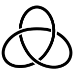
Figure 2: The trefoil knot

5.4 Example: trefoil knot

In this section, we consider the trefoil knot. The corresponding quiver has three vertices, and depending on which vertex we use as the framed vertex, we can have three different vacuum representations. For all of them, the refinement prescription (306) together with (158) applies, namely, we can always find the $\Upsilon$-charge assignment on the arrows such that the refined vacuum characters reproduce the motivic DT invariants computed via (296) and hence the LMOV invariants.

5.4.1 Quiver from trefoil knot

Via the knot-quiver correspondence, for the trefoil knot shown in Fig. 2, the quiver and its adjacency matrix are Kucharski:2017poe ; Kucharski:2017ogk :

$$Q_{\textrm{trefoil}}=\begin{array}[]{c}\leavevmode\hbox to152.01pt{\vbox to84.35pt{\text{[drawing]}}}\end{array}\,,\qquad\bm{C}=\begin{pmatrix}0&1&1\\ 1&2&2\\ 1&2&3\end{pmatrix}\,, 0 1 2 0 1 2$$ (352)

and $W=0$. Note that there are two arrows from vertex $1$ to $2$ and two from $2$ back to $1$. From the adjacency matrix in (352), one can compute the generating function of the motivic DT invariants via (296):

$$\bm{\Omega}(y,\bm{x})= \left(-x_{0}-y^{2}x_{1}+y^{3}x_{2}\right)+\left(y^{4}x_{1}^{2}+y^{8}x_{2}^{2}+y^{2}x_{0}x_{1}-y^{3}x_{0}x_{2}-(y^{5}+y^{7})x_{1}x_{2}\right)$$ (353)

$$+\left(-y^{8}x_{1}^{3}+(y^{11}+y^{13}+y^{17})x_{2}^{3}-(y^{4}+y^{6})x_{0}x_{1}^{2}-(y^{6}+y^{8}+y^{10})x_{0}x_{2}^{2}\right.$$

$$\left.\quad\,\,+(y^{7}+2y^{9}+y^{11}+y^{13})x_{1}^{2}x_{2}-(y^{8}+2y^{10}+2y^{12}+y^{14}+y^{16})x_{1}x_{2}^{2}\right.$$

$$\qquad\qquad\qquad\qquad\qquad\qquad\qquad\qquad\qquad\quad\,\left.+(2y^{5}+2y^{7}+y^{9})x_{0}x_{1}x_{2}\right)+\mathcal{O}(\bm{x}^{4})\,.$$

From the quiver (352), one can immediately read off the bonding factors (11); and plugging them into (12) one has the quiver Yangian for (352). We now check that there exists a refinement prescription for $\upsilon({\mbox{\raisebox{-0.86108pt}{\hbox to0.0pt{\hbox to7.7778pt{\hss{\hbox{\mbox{\raisebox{1.50696pt}{\scriptsize$a$}}}}\hss}\hss}\hbox{{\mbox{$\Box$}}}}}})$ together with a $\Upsilon$-charge assignment on all the arrows such that the refined vacuum character reproduces the NCDT generating functions of the motivic DT invariants.

5.4.2 Representation for the trefoil knot quiver

We first construct the vacuum-like representation using the procedure of Sec. 3.2.2. To do so, we first choose a vertex out of $0,1,2$ to frame. Different choices lead to different vacuum-like representations, but all reproduce the DT invariants $\Omega_{\bm{d}}(y)$. Let us first frame the vertex $0$ to explain the computation.

In Appx. D, we explicitly construct the states up to level $4$; here we show the final result for up to level $3$:

$$\textrm{level }0:\qquad \{\varnothing\}\,;$$ (354)

$$\textrm{level }1:\qquad \{I^{(0)}\}\,;$$

$$\textrm{level }2:\qquad \{I^{(0)},\,I^{(0)}\cdot I^{0\rightarrow 1}\}\,,\{I^{(0)},\,I^{(0)}\cdot I^{0\rightarrow 2}\}\,;$$

$$\textrm{level }3:\qquad \{I^{(0)},\,I^{(0)}\cdot I^{0\rightarrow 1},\,I^{(0)}\cdot I^{0\rightarrow 1\rightarrow 0}\},\,\{I^{(0)},\,I^{(0)}\cdot I^{0\rightarrow 2},\,I^{(0)}\cdot I^{0\rightarrow 2\rightarrow 0}\}\,,$$

$$\{I^{(0)},\,I^{(0)}\cdot I^{0\rightarrow 1},\,I^{(0)}\cdot I^{0\rightarrow 1}\cdot I^{1\rightarrow 1}_{i=1,2}\},\,\{I^{(0)},\,I^{(0)}\cdot I^{0\rightarrow 2},\,I^{(0)}\cdot I^{0\rightarrow 2}\cdot I^{2\rightarrow 2}_{i=1,2,3}\}\,,$$

$$\{I^{(0)},\,I^{(0)}\cdot I^{0\rightarrow 1},\,I^{(0)}\cdot I^{0\rightarrow 1}\cdot I^{1\rightarrow 2}_{i=1,2}\}\,,\{I^{(0)},\,I^{(0)}\cdot I^{0\rightarrow 2},\,I^{(0)}\cdot I^{0\rightarrow 2}\cdot I^{2\rightarrow 1}_{i=1,2}\}\,,$$

$$\{I^{(0)},\,I^{(0)}\cdot I^{0\rightarrow 1},\,I^{(0)}\cdot I^{0\rightarrow 2}\}\,;$$

where in $I^{1\rightarrow 1}_{i=1,2}$, $I^{2\rightarrow 2}_{i=1,2,3}$, $I^{1\rightarrow 2}_{i=1,2}$, and $I^{2\rightarrow 1}_{i=1,2}$ the subscripts distinguish the different arrows that share the same initial and final points, and we have used the shorthand $I^{a\rightarrow b\rightarrow c}=I^{a\rightarrow b}\cdot I^{b\rightarrow c}$ whenever there is no ambiguity, i.e. when there is only one single arrow from $a$ to $b$ and one arrow from $b$ to $c$.

This iterative result allows us to compute the unrefined character of ${}^{(0)}\mathcal{P}$ as the power series:

$$\bm{\mathcal{Z}}^{\textrm{unref}}_{\textrm{trefoil},0}(\bm{x})= 1+x_{0}+\left(x_{0}x_{1}+x_{0}x_{1}\right)+\left(x_{0}^{2}x_{1}+x_{0}^{2}x_{2}+2\,x_{0}x_{1}^{2}+3\,x_{0}x_{2}^{2}+5\,x_{0}x_{1}x_{2}\right)$$ (355)

$$+\left(5\,x_{0}^{2}x_{1}^{2}+7\,x_{0}^{2}x_{2}^{2}+12\,x_{0}^{2}x_{1}x_{2}+5\,x_{0}x_{1}^{3}+12\,x_{0}x_{2}^{3}+21\,x_{0}x_{1}^{2}x_{2}+28\,x_{0}x_{1}x_{2}^{2}\right)+\mathcal{O}(\bm{x}^{5})\,,$$

where the subscript in $\bm{\mathcal{Z}}^{\textrm{unref}}_{\textrm{trefoil},0}(\bm{x})$ indicates that the framed vertex is $0$. From this iterative result, one can check with Mathematica that the unrefined character of ${}^{(0)}\mathcal{P}$ reproduces

$$\bm{\mathcal{Z}}^{\textrm{unref}}_{\textrm{trefoil},0}(\bm{x}) =\widehat{\textrm{Sgn}}\cdot\textrm{PE}\left[\sum_{\bm{d}}d_{0}\,\Omega_{\bm{d}}(1)\bm{x}^{\bm{d}}\right]\,,$$ (356)

where

$$\widehat{\textrm{Sgn}}:\qquad x_{0}\rightarrow-x_{0}\,,x_{1}\rightarrow-x_{1}$$ (357)

and $\Omega_{d}(1)$ are the numerical DT invariants computed from (296) using the adjacency matrix $\bm{C}$ in (352) and setting $y=1$.

5.4.3 Refined characters of vacuum-like representations

Now we describe a refinement prescription such that the refined characters of all the vacuum-like representations reproduce the motivic DT invariants computed from (296) using the adjacency matrix $\bm{C}$ in (352).

Recall that for the $m$-loop quiver, the refinement prescription on $\upsilon({\mbox{\raisebox{-0.86108pt}{\hbox to0.0pt{\hbox to7.7778pt{\hss{\hbox{\mbox{\raisebox{1.50696pt}{\scriptsize$0$}}}}\hss}\hss}\hbox{{\mbox{$\Box$}}}}}})$ is given by (327). Since the $m$-loop quivers can be considered as the building blocks for the symmetric quivers without potential Jankowski:2022qdp , when there is more than one vertex, it is natural to generalize (327) to

$$\upsilon({\mbox{\raisebox{-0.86108pt}{\hbox to0.0pt{\hbox to7.7778pt{\hss{\hbox{\mbox{\raisebox{1.50696pt}{\scriptsize$a$}}}}\hss}\hss}\hbox{{\mbox{$\Box$}}}}}})=\delta_{a\in Q_{0}^{\prime}}\cdot\Upsilon({\mbox{\raisebox{-0.86108pt}{\hbox to0.0pt{\hbox to7.7778pt{\hss{\hbox{\mbox{\raisebox{1.50696pt}{\scriptsize$a$}}}}\hss}\hss}\hbox{{\mbox{$\Box$}}}}}})\qquad\textrm{with}\quad\Upsilon({\mbox{\raisebox{-0.86108pt}{\hbox to0.0pt{\hbox to7.7778pt{\hss{\hbox{\mbox{\raisebox{1.50696pt}{\scriptsize$a$}}}}\hss}\hss}\hbox{{\mbox{$\Box$}}}}}})=\sum_{I\in\mathfrak{p}^{\infty\rightarrow a}}\Upsilon(I)\,,$$ (358)

where $\delta_{a}=1$ when $a$ is in the subset $Q_{0}^{\prime}\subset Q_{0}$ to be determined, otherwise 0. (The final result for (358) was already summarized in the second line of (306).) We will confirm the ansatz (358) with explicit computations later.

Next, in the quiver (352), let us label the charges for the $i^{\textrm{th}}$ arrows from $a$ to $b$ by $\Upsilon_{i}^{a\rightarrow b}$; in this case we have $13$ parameters to determine:

$$\Upsilon_{i=1,2}^{1\rightarrow 1}\,,\quad\Upsilon_{i=1,2,3}^{2\rightarrow 2}\,,\quad\Upsilon^{0\rightarrow 1}\,,\quad\Upsilon^{1\rightarrow 0}\,,\quad\Upsilon^{0\rightarrow 2}\,,\quad\Upsilon^{2\rightarrow 0},\quad\Upsilon_{i=1,2}^{1\rightarrow 2}\,,\quad\Upsilon_{i=1,2}^{2\rightarrow 1}\,.$$ (359)

The goal is to fix these $13$ parameters, together with the subset $Q_{0}^{\prime}$, in such a way that the resulting refined vacuum character $\bm{\mathcal{Z}}^{\textrm{ref}}_{\textrm{trefoil},\mathfrak{a}}(y,\bm{x})$, as computed from definition (156) with prescription (358), agrees with $\widehat{\textrm{Sgn}}\cdot\mathcal{Z}_{\textrm{NC},\mathfrak{a}}(y,\bm{x})$, as computed from (308) and (296) and with $\widehat{\textrm{Sgn}}$ given by (357):

$$\bm{\mathcal{Z}}^{\textrm{ref}}_{\textrm{trefoil},\mathfrak{a}}(y,\bm{x})=\left(\sum_{\Pi\in{}^{(\mathfrak{a})}\mathcal{P}}y^{\upsilon(\Pi)}\,\bm{x}^{|\Pi|}\right)=\widehat{\textrm{Sgn}}\cdot\mathcal{Z}_{\textrm{NC},\mathfrak{a}}(y,\bm{x})=\widehat{\textrm{Sgn}}\cdot\textrm{PE}\left[\frac{\widehat{\bm{\Omega}}_{\mathfrak{a}}(y,\bm{x})}{y^{2}-1}\right]\,.$$ (360)

In (360), the subscript $\mathfrak{a}$ denotes the choice of the framed vertex in the canonical framing; it enters ${}^{(\mathfrak{a})}\mathcal{P}$ as the color of the leading atom $\mathfrak{a}$$\Box$, and $\widehat{\bm{\Omega}}_{\mathfrak{a}}(y,\bm{x})$ via its definition (308) that depends on $\mathfrak{a}$ explicitly. Therefore, a priori the solution for the subset $Q_{0}^{\prime}$ and the $13$ parameters in (359) depends on the choice of $\mathfrak{a}$.

Let us first consider the case with $\mathfrak{a}=0$. We leave the details to Appx. D. The final result is that, when $\mathfrak{a}=0$, with the prescription for step 3 of the refinement procedure (explained in Sec. 4.2) given by

$$\upsilon({\mbox{\raisebox{-0.86108pt}{\hbox to0.0pt{\hbox to7.7778pt{\hss{\hbox{\mbox{\raisebox{1.50696pt}{\scriptsize$0$}}}}\hss}\hss}\hbox{{\mbox{$\Box$}}}}}})=0\quad\textrm{and}\quad \upsilon({\mbox{\raisebox{-0.86108pt}{\hbox to0.0pt{\hbox to7.7778pt{\hss{\hbox{\mbox{\raisebox{1.50696pt}{\scriptsize$a$}}}}\hss}\hss}\hbox{{\mbox{$\Box$}}}}}})=\Upsilon({\mbox{\raisebox{-0.86108pt}{\hbox to0.0pt{\hbox to7.7778pt{\hss{\hbox{\mbox{\raisebox{1.50696pt}{\scriptsize$a$}}}}\hss}\hss}\hbox{{\mbox{$\Box$}}}}}})\equiv\sum_{I\in\mathfrak{p}^{\infty\rightarrow a}}\Upsilon(I)\qquad a=1,2$$ (361)

namely $Q_{0}^{\prime}=\{1,2\}$, we find a unique $\Upsilon$-charge assignment

$$^{\sharp}Q_{\textrm{trefoil},0}=\begin{array}[]{c}\leavevmode\hbox to183.67pt{\vbox to99.32pt{\text{[drawing]}}}\end{array} 0 \infty 1 2 0 0,2 0,2,4 2 2 1,3 1,3 3 3$$ (362)

More explicitly, in Appx. D we determine the prescription (361) and the $\Upsilon$-charge assignment (362) by matching $\bm{\mathcal{Z}}^{\textrm{ref}}_{\textrm{trefoil},0}(y,\bm{x})$, as computed from definition (156) with prescription (361), to $\widehat{\textrm{Sgn}}\cdot\mathcal{Z}_{\textrm{NC},0}(y,\bm{x})$, as computed from (308) and (296), up to level $4$:

$$\bm{\mathcal{Z}}^{\textrm{ref}}_{\textrm{trefoil},0}(y,\bm{x})=\widehat{\textrm{Sgn}}\cdot\mathcal{Z}_{\textrm{NC},0}(y,\bm{x})$$ (363)

$$=1+x_{0}+\left(y^{2}x_{0}x_{1}+y^{3}x_{0}x_{2}\right)$$

$$\quad+\left(y^{2}x_{0}^{2}x_{1}+y^{3}x_{0}^{2}x_{2}+(y^{4}+y^{6})\,x_{0}x^{2}_{1}+(y^{6}+y^{8}+y^{10})\,x_{0}x_{2}^{2}+(2y^{5}+2y^{7}+y^{9})\,x_{0}x_{1}x_{2}\right)$$

$$\quad+\left((2y^{4}+2y^{6}+y^{8})\,x_{0}^{2}x_{1}^{2}+(2y^{6}+2y^{8}+2y^{10}+y^{12})\,x_{0}^{2}x_{2}^{2}+(4y^{5}+4y^{7}+3y^{9}+y^{11})\,x_{0}^{2}x_{1}x_{2}\right.$$

$$\quad\qquad+(y^{6}+2y^{8}+y^{10}+y^{12})\,x_{0}x_{1}^{3}+(y^{9}+2y^{11}+3y^{13}+2y^{15}+2y^{17}+y^{19}+y^{21})\,x_{0}x_{2}^{3}$$

$$\quad\qquad\qquad\qquad\qquad\qquad\qquad+(3y^{7}+6y^{9}+5y^{11}+4y^{13}+2y^{15}+y^{17})\,x_{0}x_{1}^{2}x_{2}$$

$$\quad\qquad\left.\qquad\qquad\qquad\qquad\qquad+(3y^{8}+6y^{10}+7y^{12}+5y^{14}+4y^{16}+2y^{18}+y^{20})\,x_{0}x_{1}x_{2}^{2}\right)+\mathcal{O}(\bm{x}^{5})\,.$$

One then uses Mathematica to check that this assignment reproduces also the higher order terms in the expansion of $\widehat{\textrm{Sgn}}\cdot\mathcal{Z}_{\textrm{NC},0}(y,\bm{x})$. Note that since the refined character contains an infinite number of terms, the fact that the charges fixed at low orders allow the identity (360) is non-trivial.

As a consistency check, we have also done this computation for the other two canonical framings $\mathfrak{a}=1,2$. Let us first consider how the framing choice $\mathfrak{a}$ enters the computation. The partition function $\mathcal{Z}_{\textrm{NC},\mathfrak{a}}(y,\bm{x})$ computed from (308) starts with

$$\mathcal{Z}_{\textrm{NC},\mathfrak{a}}(y,\bm{x})=1+\Omega_{\bm{f}_{\mathfrak{a}}}(y)+\cdots\,,$$ (364)

where $\bm{f}_{\mathfrak{a}}$ is the framing vector $\textrm{e}_{\mathfrak{a}}$. In this case, there are three possible framing vectors $\bm{f}_{0}=(1,0,0)$, $\bm{f}_{1}=(0,1,0)$, $\bm{f}_{2}=(0,0,1)$, corresponding to $\mathfrak{a}=0,1,2$, respectively. From the leading terms in (353):

$$\bm{\Omega}(y,\bm{x})=-x_{0}-y^{2}x_{1}+y^{3}x_{2}+\mathcal{O}(\bm{x}^{2})\,,$$ (365)

we have

$$\mathcal{Z}_{\textrm{NC},\mathfrak{a}}(y,\bm{x})=\begin{cases}\begin{aligned} &1-x_{0}+\mathcal{O}(\bm{x}^{2})\quad\qquad\textrm{for}\quad\mathfrak{a}=0\,,\\ &1-y^{2}x_{1}+\mathcal{O}(\bm{x}^{2})\qquad\textrm{for}\quad\mathfrak{a}=1\,,\\ &1+y^{3}x_{2}+\mathcal{O}(\bm{x}^{2})\qquad\textrm{for}\quad\mathfrak{a}=2\,,\\ \end{aligned}\end{cases}$$ (366)

which can be collectively written as

$$\widehat{\textrm{Sgn}}\cdot\mathcal{Z}_{\textrm{NC},\mathfrak{a}}(y,\bm{x})=1+y^{m_{\mathfrak{a}}}x_{\mathfrak{a}}+\cdots\,,$$ (367)

where $\widehat{\textrm{Sgn}}$ was defined in (357), $x_{\mathfrak{a}}$ is the fugacity for the framed vertex $\mathfrak{a}$, and $m_{\mathfrak{a}}$ is the number of self-loops at vertex $\mathfrak{a}$. Therefore, the $\Upsilon$-charge for the arrow $I^{\infty\rightarrow\mathfrak{a}}$ from the framing node $\infty$ to the framed node $\mathfrak{a}$ is

$$\Upsilon^{\infty\rightarrow\mathfrak{a}}\equiv\Upsilon(I^{\infty\rightarrow\mathfrak{a}})=m_{\mathfrak{a}}\,.$$ (368)

Since the arrow $I^{\infty\rightarrow\mathfrak{a}}$ is the first arrow in all atoms, it is convenient to define a shift in the variable $x_{\mathfrak{a}}$:

$$\hat{\textrm{S}}_{\mathfrak{a}}:\qquad x_{\mathfrak{a}}\rightarrow y^{-m_{\mathfrak{a}}}\,x_{\mathfrak{a}}\,,$$ (369)

under which

$$\accentset{\circ}{\bm{\mathcal{Z}}}^{\textrm{ref}}_{\textrm{trefoil},\mathfrak{a}}(y,\bm{x})\equiv\hat{\textrm{S}}_{\mathfrak{a}}\cdot\bm{\mathcal{Z}}^{\textrm{ref}}_{\textrm{trefoil},\mathfrak{a}}(y,\bm{x})=\widehat{\textrm{S}}_{\mathfrak{a}}\cdot\widehat{\textrm{Sgn}}\cdot\mathcal{Z}_{\textrm{NC},\mathfrak{a}}(y,\bm{x})=1+x_{\mathfrak{a}}+\cdots\,.$$ (370)

Namely, the only difference between $\accentset{\circ}{\bm{\mathcal{Z}}}^{\textrm{ref}}_{\textrm{trefoil},\mathfrak{a}}(y,\bm{x})$ and $\bm{\mathcal{Z}}^{\textrm{ref}}_{\textrm{trefoil},\mathfrak{a}}(y,\bm{x})$ is that for the former $I^{\infty\rightarrow\mathfrak{a}}=0$ and for the latter $I^{\infty\rightarrow\mathfrak{a}}=m_{\mathfrak{a}}$. Then in practice, one can first try to match $\accentset{\circ}{\bm{\mathcal{Z}}}^{\textrm{ref}}_{\textrm{trefoil},\mathfrak{a}}(y,\bm{x})$ with $\widehat{\textrm{S}}_{\mathfrak{a}}\cdot\widehat{\textrm{Sgn}}\cdot\mathcal{Z}_{\textrm{NC},\mathfrak{a}}(y,\bm{x})$ by setting $\Upsilon^{\infty\rightarrow\mathfrak{a}}=0$ and determining the subset $Q_{0}^{\prime}$ in the prescription (358) together with the charges in (359). The final solution then has the same solution for $Q_{0}^{\prime}$ and all the charges in (359) together with $I^{\infty\rightarrow\mathfrak{a}}=m_{\mathfrak{a}}$.

We omit the details and only quote the final result. For the framed vertex $\mathfrak{a}=1$, we find that the procedure above fixes the prescription

$$\upsilon({\mbox{\raisebox{-0.86108pt}{\hbox to0.0pt{\hbox to7.7778pt{\hss{\hbox{\mbox{\raisebox{1.50696pt}{\scriptsize$1$}}}}\hss}\hss}\hbox{{\mbox{$\Box$}}}}}})=0\quad\textrm{and}\quad \upsilon({\mbox{\raisebox{-0.86108pt}{\hbox to0.0pt{\hbox to7.7778pt{\hss{\hbox{\mbox{\raisebox{1.50696pt}{\scriptsize$a$}}}}\hss}\hss}\hbox{{\mbox{$\Box$}}}}}})=\Upsilon({\mbox{\raisebox{-0.86108pt}{\hbox to0.0pt{\hbox to7.7778pt{\hss{\hbox{\mbox{\raisebox{1.50696pt}{\scriptsize$a$}}}}\hss}\hss}\hbox{{\mbox{$\Box$}}}}}})\equiv\sum_{I\in\mathfrak{p}^{\infty\rightarrow a}}\Upsilon(I)\qquad a=0,2$$ (371)

and the $\Upsilon$-charge assignment for the arrows

$$^{\sharp}Q_{\textrm{trefoil},1}=\begin{array}[]{c}\leavevmode\hbox to183.67pt{\vbox to116.08pt{\text{[drawing]}}}\end{array} 0 \infty 1 2 2 0,2 0,2,4 4-\alpha \alpha 3,5 -1,1 7-\alpha \alpha-1$$ (372)

where $\alpha=\Upsilon(I^{1\rightarrow 0})$. Similar to the case with $\mathfrak{a}=0$, the $\Upsilon$-charge assignment (372) is determined by matching $\accentset{\circ}{\bm{\mathcal{Z}}}^{\textrm{ref}}_{\textrm{trefoil},1}(y,\bm{x})$ with $\widehat{\textrm{S}}_{\texttt{1}}\cdot\widehat{\textrm{Sgn}}\cdot\mathcal{Z}_{\textrm{NC},1}(y,\bm{x})$ up to level $4$, and for which we give the first three levels here

$$\accentset{\circ}{\bm{\mathcal{Z}}}^{\textrm{ref}}_{\textrm{trefoil},1}(y,\bm{x}) =1+x_{1}+\left(x_{0}x_{1}+(1+y^{2})x_{1}^{2}+(y^{3}+y^{5})x_{1}x_{2}\right)$$ (373)

$$\,\,\,+\left((1+2y^{2}+y^{4}+y^{6})x_{1}^{3}+(2+2y^{2}+y^{4})x_{0}x_{1}^{2}+(2y^{3}+2y^{5}+y^{7})x_{0}x_{1}x_{2}\right.$$

$$\,\quad\,\,\left.+(2y^{3}+4y^{5}+3y^{7}+2y^{9}+y^{11})x_{1}^{2}x_{2}+(y^{6}+2y^{8}+2y^{10}+y^{12}+y^{14})x_{1}x_{2}^{2}\right)+\mathcal{O}(\bm{x}^{4})\,.$$

One can then use Mathematica to check that the assignment (372) reproduces also the higher order terms in the expansion of $\widehat{\textrm{S}}_{\texttt{1}}\cdot\widehat{\textrm{Sgn}}\cdot\mathcal{Z}_{\textrm{NC},1}(y,\bm{x})$. Note that since the atom of color $0$ doesn’t contribute to the $\Upsilon$-charge, and in the expansion (373), $\Upsilon^{0\rightarrow 1,2}$ and $\Upsilon^{1,2\rightarrow 0}$ always appear in the pairs

$$\Upsilon^{1\rightarrow 0}+\Upsilon^{0\rightarrow 1}\,,\quad\Upsilon^{1\rightarrow 0}+\Upsilon^{0\rightarrow 2}\,,\quad\Upsilon^{2\rightarrow 0}+\Upsilon^{0\rightarrow 2}\,,\quad\Upsilon^{2\rightarrow 0}+\Upsilon^{0\rightarrow 1}\,,$$ (374)

there is one free parameter in the assignment (372).

Similarly, for the framed vertex $\mathfrak{a}=2$, the procedure above fixes the prescription

$$\upsilon({\mbox{\raisebox{-0.86108pt}{\hbox to0.0pt{\hbox to7.7778pt{\hss{\hbox{\mbox{\raisebox{1.50696pt}{\scriptsize$2$}}}}\hss}\hss}\hbox{{\mbox{$\Box$}}}}}})=0\quad\textrm{and}\quad \upsilon({\mbox{\raisebox{-0.86108pt}{\hbox to0.0pt{\hbox to7.7778pt{\hss{\hbox{\mbox{\raisebox{1.50696pt}{\scriptsize$a$}}}}\hss}\hss}\hbox{{\mbox{$\Box$}}}}}})=\Upsilon({\mbox{\raisebox{-0.86108pt}{\hbox to0.0pt{\hbox to7.7778pt{\hss{\hbox{\mbox{\raisebox{1.50696pt}{\scriptsize$a$}}}}\hss}\hss}\hbox{{\mbox{$\Box$}}}}}})\equiv\sum_{I\in\mathfrak{p}^{\infty\rightarrow a}}\Upsilon(I)\qquad a=0,1$$ (375)

and the $\Upsilon$-charge assignment for the arrows

$$^{\sharp}Q_{\textrm{trefoil},2}=\begin{array}[]{c}\leavevmode\hbox to183.67pt{\vbox to116.08pt{\text{[drawing]}}}\end{array} 0 \infty 1 2 3 0,2 0,2,4 4-\alpha \alpha 0,2 2,4 4-\alpha 2+\alpha$$ (376)

where $\alpha=\Upsilon(I^{1\rightarrow 0})$. Again, the $\Upsilon$-charge assignment (376) is determined by matching $\accentset{\circ}{\bm{\mathcal{Z}}}^{\textrm{ref}}_{\textrm{trefoil},2}(y,\bm{x})$ with $\widehat{\textrm{S}}_{\texttt{2}}\cdot\widehat{\textrm{Sgn}}\cdot\mathcal{Z}_{\textrm{NC},2}(y,\bm{x})$ up to level $4$, and for which we give the first three levels here

$$\accentset{\circ}{\bm{\mathcal{Z}}}^{\textrm{ref}}_{\textrm{trefoil},2}(y,\bm{x})= 1+x_{2}+\left((1+y^{2}+y^{4})x_{2}^{2}+x_{0}x_{2}+(y^{2}+y^{4})x_{1}x_{2}\right)$$ (377)

$$+\left((1+2y^{2}+3y^{4}+2y^{6}+2y^{8}+y^{10}+y^{12})x_{2}^{3}+(2+2y^{2}+2y^{4}+y^{6})x_{0}x_{2}^{2}\right.$$

$$\quad+(2y^{2}+4y^{4}+4y^{6}+3y^{8}+2y^{10}+y^{12})x_{1}x_{2}^{2}+(y^{4}+2y^{6}+y^{8}+y^{10})x_{1}^{2}x_{2}$$

$$\left.\qquad\qquad\qquad\qquad\qquad\qquad\qquad\qquad\qquad\qquad+(2y^{2}+2y^{4}+y^{6})x_{0}x_{1}x_{2}\right)+\mathcal{O}(\bm{x}^{4})\,.$$

One can then use Mathematica to check that the assignment (376) also reproduces the higher order terms in the expansion of $\widehat{\textrm{S}}_{\texttt{2}}\cdot\widehat{\textrm{Sgn}}\cdot\mathcal{Z}_{\textrm{NC},2}(y,\bm{x})$.

Finally, we observe that in all three cases, the charges satisfy

$$\Upsilon^{0\rightarrow 1}+\Upsilon^{1\rightarrow 0}=4\,,\quad\Upsilon^{0\rightarrow 2}+\Upsilon^{2\rightarrow 0}=6\,,\quad\sum^{2}_{j=1}(\Upsilon_{j}^{1\rightarrow 2}+\Upsilon_{j}^{2\rightarrow 1})=8\,.$$ (378)

5.5 Example: Hopf link

As a final example, let us consider the Hopf link, shown in Figure 3

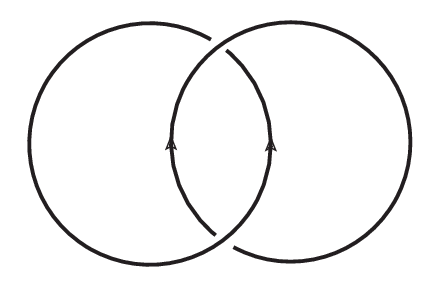
Figure 3: Hopf link

5.5.1 Quiver for Hopf link

In the knot-quiver correspondence, the quiver that corresponds to the Hopf link and its adjacency matrix are Kucharski:2017poe ; Kucharski:2017ogk :

$$Q_{\textrm{Hopf link}}=\begin{array}[]{c}\leavevmode\hbox to113.32pt{\vbox to108.81pt{\text{[drawing]}}}\end{array}\,,\qquad\bm{C}_{\textrm{Hopf link}}=\begin{pmatrix}0&0&1&1\\ 0&1&1&1\\ 1&1&3&2\\ 1&1&2&2\end{pmatrix}\,, 0 1 2 3 0 1 2 3$$ (379)

and $W=0$. Note that there are two arrows from vertex $2$ to $3$ and two from $3$ back to $2$. From the adjacency matrix in (379), one can compute the generating function of the motivic DT invariants via (296) using the adjacency matrix $\bm{C}$ in (379):

$$\bm{\Omega}(y,\bm{x})= \left(-x_{0}+yx_{1}-y^{2}x_{3}+y^{3}x_{2}\right)$$ (380)

$$+\left(-y^{3}x_{0}x_{2}+y^{2}x_{0}x_{3}-y^{3}x_{1}x_{3}+y^{4}x_{1}x_{2}+y^{4}x_{3}^{2}+y^{8}x_{2}^{2}-(y^{5}+y^{7})x_{2}x_{3}\right)$$

$$+\left((y^{11}+y^{13}+y^{17})x_{2}^{3}-y^{8}x_{3}^{3}-(y^{6}+y^{8}+y^{10})x_{0}x_{2}^{2}-(y^{4}+y^{6})x_{0}x_{3}^{2}+y^{5}x_{1}^{2}x_{2}-y^{4}x_{1}^{2}x_{3}\right.$$

$$\quad\,\,+(y^{7}+y^{9}+y^{11})x_{1}x_{2}^{2}+(y^{5}+y^{7})x_{1}x_{3}^{2}-(y^{8}+2y^{10}+2y^{12}+y^{14}+y^{16})x_{2}^{2}x_{3}$$

$$\quad\,\,+(y^{7}+2y^{9}+y^{11}+y^{13})x_{2}x_{3}^{2}-y^{4}x_{0}x_{1}x_{2}+(2y^{5}+2y^{7}+y^{9})x_{0}x_{2}x_{3}+y^{3}x_{0}x_{1}x_{3}$$

$$\quad\qquad\qquad\qquad\qquad\qquad\qquad\qquad\qquad\qquad\qquad\quad-(2y^{6}+2y^{8}+y^{10})x_{1}x_{2}x_{3})+\mathcal{O}(\bm{x}^{4})\,.$$

From the quiver (379), one can immediately read off the bonding factors (11); and plugging them into (12) one has the quiver Yangian for (379). We now check that the refined vacuum character gives the NCDT generating function of the motivic DT invariants.

5.5.2 Representation for Hopf link quiver

To construct the vacuum-like representation using the procedure of Sec. 3.2.2, we first choose a vertex out of $0,1,2,3$ to frame. Let us frame the vertex $0$ to explain the computation. Note that the assignment of $\Upsilon$-charge to the arrows depends on the choice of the framing.

We skip the details and give the final result for first few levels.

$$\textrm{level }0:\qquad \{\varnothing\}\,;$$ (381)

$$\textrm{level }1:\qquad \{I^{(0)}\}\,;$$

$$\textrm{level }2:\qquad \{I^{(0)},\,I^{(0)}\cdot I^{0\rightarrow 2}\}\,,\{I^{(0)},\,I^{(0)}\cdot I^{0\rightarrow 3}\}\,;$$

$$\textrm{level }3:\qquad \{I^{(0)},\,I^{(0)}\cdot I^{0\rightarrow 2},\,I^{(0)}\cdot I^{0\rightarrow 2\rightarrow 0}\},\,\{I^{(0)},\,I^{(0)}\cdot I^{0\rightarrow 3},\,I^{(0)}\cdot I^{0\rightarrow 3\rightarrow 0}\}\,,$$

$$\{I^{(0)},\,I^{(0)}\cdot I^{0\rightarrow 2},\,I^{(0)}\cdot I^{0\rightarrow 2\rightarrow 1}\},\,\{I^{(0)},\,I^{(0)}\cdot I^{0\rightarrow 3},\,I^{(0)}\cdot I^{0\rightarrow 3\rightarrow 1}\}\,,$$

$$\{I^{(0)},\,I^{(0)}\cdot I^{0\rightarrow 2},\,I^{(0)}\cdot I^{0\rightarrow 2}\cdot I^{2\rightarrow 2}_{i=1,2,3}\},\,\{I^{(0)},\,I^{(0)}\cdot I^{0\rightarrow 3},\,I^{(0)}\cdot I^{0\rightarrow 3}\cdot I^{3\rightarrow 3}_{i=1,2}\}\,,$$

$$\{I^{(0)},\,I^{(0)}\cdot I^{0\rightarrow 2},\,I^{(0)}\cdot I^{0\rightarrow 2}\cdot I^{3\rightarrow 2}_{i=1,2}\}\,,\{I^{(0)},\,I^{(0)}\cdot I^{0\rightarrow 3},\,I^{(0)}\cdot I^{0\rightarrow 3}\cdot I^{3\rightarrow 2}_{i=1,2}\}\,,$$

$$\{I^{(0)},\,I^{(0)}\cdot I^{0\rightarrow 2},\,I^{(0)}\cdot I^{0\rightarrow 3}\}\,;$$

where in $I^{2\rightarrow 2}_{i=1,2,3}$, $I^{3\rightarrow 3}_{i=1,2}$, $I^{2\rightarrow 3}_{i=1,2}$, and $I^{3\rightarrow 2}_{i=1,2}$ the subscripts distinguish the different arrows that share the same initial and final points, and we have used the shorthand $I^{a\rightarrow b\rightarrow c}=I^{a\rightarrow b}\cdot I^{b\rightarrow c}$ whenever there is no ambiguity, i.e. when there is only one single arrow from $a$ to $b$ and one arrow from $b$ to $c$.

This iterative result allows us to compute the unrefined vacuum character as a power series:

$$\bm{\mathcal{Z}}^{\textrm{unref}}_{\textrm{hopf link},0}(\bm{x})= 1+x_{0}+\left(x_{0}x_{2}+x_{0}x_{3}\right)$$ (382)

$$+\left(x_{0}^{2}x_{2}+x_{0}^{2}x_{3}+3\,x_{0}x_{2}^{2}+2\,x_{0}x_{3}^{2}+x_{0}x_{1}x_{2}+x_{0}x_{1}x_{3}+5\,x_{0}x_{2}x_{3}\right)$$

$$+\left(7x_{0}^{2}x_{2}^{2}+5x_{0}^{2}x_{3}^{2}+x_{0}^{2}x_{1}x_{2}+x_{0}^{2}x_{1}x_{3}+12x_{0}^{2}x_{2}x_{3}+x_{0}x_{1}^{2}x_{2}+7x_{0}x_{1}x_{2}^{2}+12x_{0}x_{2}^{3}\right.$$

$$\qquad\left.+5x_{0}x_{3}^{3}+x_{0}x_{1}^{2}x_{3}+28x_{0}x_{2}^{2}x_{3}+5x_{0}x_{1}x_{3}^{2}+12x_{0}x_{1}x_{2}x_{3}+21x_{0}x_{2}x_{3}^{2}\right)+\mathcal{O}(\bm{x}^{5})\,.$$

From this iterative result, one can check with Mathematica that the unrefined vacuum character reproduces

$$\bm{\mathcal{Z}}^{\textrm{unref}}_{\textrm{hopf link},0}(\bm{x}) =\widehat{\textrm{Sgn}}\cdot\textrm{PE}\left[\sum_{\bm{d}}d_{0}\,\Omega_{\bm{d}}(1)\bm{x}^{\bm{d}}\right]\,,$$ (383)

where

$$\widehat{\textrm{Sgn}}:\qquad x_{0}\rightarrow-x_{0}\,,\quad x_{3}\rightarrow-x_{3}$$ (384)

and $\Omega_{d}(1)$ are the numerical DT invariants that can be computed from (296) using the adjacency matrix $\bm{C}$ in (379) and setting $y=1$.

5.5.3 Refined vacuum character

Now we describe a refinement prescription that reproduces the motivic DT invariants computed from (296), using a computation that is parallel to the one in Appx. D for the trefoil knot. We fix the refinement prescription

$$\upsilon({\mbox{\raisebox{-0.86108pt}{\hbox to0.0pt{\hbox to7.7778pt{\hss{\hbox{\mbox{\raisebox{1.50696pt}{\scriptsize$0$}}}}\hss}\hss}\hbox{{\mbox{$\Box$}}}}}})=0\quad\textrm{and}\quad \upsilon({\mbox{\raisebox{-0.86108pt}{\hbox to0.0pt{\hbox to7.7778pt{\hss{\hbox{\mbox{\raisebox{1.50696pt}{\scriptsize$a$}}}}\hss}\hss}\hbox{{\mbox{$\Box$}}}}}})=\Upsilon({\mbox{\raisebox{-0.86108pt}{\hbox to0.0pt{\hbox to7.7778pt{\hss{\hbox{\mbox{\raisebox{1.50696pt}{\scriptsize$a$}}}}\hss}\hss}\hbox{{\mbox{$\Box$}}}}}})\equiv\sum_{I\in\mathfrak{p}^{0\rightarrow a}}\Upsilon(I)\qquad a=1,2,3\,,$$ (385)

which was already summarized in the second line of (306), and assign to the arrows the $\Upsilon$ charges:

$$^{\sharp}Q=\begin{array}[]{c}\leavevmode\hbox to190.19pt{\vbox to154.33pt{\text{[drawing]}}}\end{array} 0 \infty 1 2 3 0 3 3 2 2 -2 4 3 -1 1,3 1,3 0 0,2,4 0,2$$ (386)

The $\Upsilon$-charge assignment (386) is determined by matching $\bm{\mathcal{Z}}^{\textrm{ref}}_{\textrm{Hopf link},0}(y,\bm{x})$ with $\widehat{\textrm{Sgn}}\cdot\mathcal{Z}_{\textrm{NC},0}(y,\bm{x})$ up to level $4$:

$$\bm{\mathcal{Z}}^{\textrm{ref}}_{\textrm{Hopf link},0}(y,\bm{x})=\widehat{\textrm{Sgn}}\cdot\mathcal{Z}_{\textrm{NC}}(y,\bm{x})$$ (387)

$$=1+x_{0}+\left(y^{3}x_{0}x_{2}+y^{2}x_{0}x_{3}\right)$$

$$\quad+\left(y^{3}x_{0}^{2}x_{2}+y^{2}x_{0}^{2}x_{3}+y^{4}x_{0}x_{1}x_{2}+y^{3}x_{0}x_{1}x_{3}+(y^{6}+y^{8}+y^{10})x_{0}x_{2}^{2}\right.$$

$$\quad\,\,\left.\,\qquad\qquad\qquad\qquad\qquad+(y^{4}+y^{6})x_{0}x_{3}^{2}+(2y^{5}+2y^{7}+y^{9})x_{0}x_{2}x_{3}\right)$$

$$\quad+\left((2y^{6}+2y^{8}+2y^{10}+y^{12})x_{0}^{2}x_{2}^{2}+(2y^{4}+2y^{6}+y^{8})x_{0}^{2}x_{3}^{2}+(y^{6}+2y^{8}+y^{10}+y^{12})x_{0}x_{3}^{3}\right.$$

$$\quad\quad\,\,+(y^{9}+2y^{11}+3y^{13}+2y^{15}+2y^{17}+y^{19}+y^{21})x_{0}x_{2}^{3}+(4y^{5}+4y^{7}+3y^{9}+y^{11})x_{0}^{2}x_{2}x_{3}$$

$$\quad\quad\,\,+y^{4}x_{0}^{2}x_{1}x_{2}+y^{3}x_{0}^{2}x_{1}x_{3}+y^{5}x_{0}x_{1}^{2}x_{2}+y^{4}x_{0}x_{1}^{2}x_{3}+(2y^{7}+2y^{9}+2y^{11}+y^{13})x_{0}x_{1}x_{2}^{2}$$

$$\quad\quad\,\,+(2y^{5}+2y^{7}+y^{9})x_{0}x_{1}x_{3}^{2}+(3y^{8}+6y^{10}+7y^{12}+5y^{14}+4y^{16}+2y^{18}+y^{20})x_{0}x_{2}^{2}x_{3}$$

$$\quad\quad\,\left.+(3y^{7}+6y^{9}+5y^{11}+4y^{13}+2y^{15}+y^{17})x_{0}x_{2}x_{3}^{2}+(4y^{6}+4y^{8}+3y^{10}+y^{12})x_{0}x_{1}x_{2}x_{3}\right)+\mathcal{O}(\bm{x}^{5})\,.$$

We have checked that the assignment (386) reproduces higher order terms in the expansion of $\widehat{\textrm{Sgn}}\cdot\mathcal{Z}_{\textrm{NC},0}(y,\bm{x})$ with $\widehat{\textrm{Sgn}}$ given by (384). The cases with framing $\mathfrak{a}=1,2,3$ work in a similar way, and we omit the details here.

6 Summary and Discussion

In this work, we have generalized the study of quiver Yangians from the toric CY₃ quivers to general quivers. The definition of the quiver Yangian is formally unchanged. However, unlike the toric CY₃ quivers, for which the representations were known to be given by 3D colored crystals, the representations of the quiver Yangians for general quivers are unknown.

In this paper, we first described a procedure for constructing the vacuum representation for an arbitrary quiver Yangian, and then showed that they indeed form a representation of the quiver Yangian. We then explained how to construct arbitrary non-vacuum representations from these vacuum representations. These representations allow us to compute the characters of the quiver Yangian straightforwardly.

The construction above applies to all quivers. We then focused on two families of quivers that are particularly fascinating.

For the BPS quivers of 4D $\mathcal{N}=2$ theories, the quiver Yangians are the BPS algebras of these systems. Besides the toric CY₃ quivers, we studied as examples the Kronecker quivers and affine ADE quivers and computed the vacuum characters of these quiver Yangians, which map to the BPS partition functions and generating functions of the framed DT invariants (in the NCDT chamber) of these systems. We also studied the refinement of the vacuum characters in order to reproduce the refined BPS partition functions of the framed motivic DT invariants. While the refinement choice is not unique, we gave one simple and universal refinement procedure and also discussed various other choices.

For the quivers that come from the knot-quiver correspondence, we conjecture that the quiver Yangians are the BPS algebras for the underlying 3D $\mathcal{N}=2$ theory of Ekholm:2018eee . As examples of this type of quivers, we studied the $m$-loop quivers (which can be viewed as the building block of these knot quivers), the trefoil knot, and the Hopf link. We found a unique refinement prescription with which the refined vacuum character of the corresponding quiver Yangian reproduces precisely the refined motivic DT invariants and hence the knot invariants by the knot-quiver correspondence. This provides strong evidence that the quiver Yangians are also the BPS algebras for the system that gives rise to the knot-quiver correspondence. Intriguingly, this refinement is slightly different from the one used for the BPS quivers of the 4D $\mathcal{N}=2$ theories.

Finally, it is straightforward to generalize these quiver Yangians for arbitrary quivers to the trigonometric, elliptic, and generalized cohomological versions, following Galakhov:2021omc , see Appx. E.

Let us list some interesting directions for future research. For the BPS quivers of the 4D $\mathcal{N}=2$ theories:

• The refined characters of the quiver Yangian offers a method to compute the framed refined DT invariants for arbitrary BPS quivers in the NCDT chamber. On the other hand, one can use the attractor tree formula of Mozgovoy:2020has ; Mozgovoy:2021iwz or the flow tree formula of Arguz:2021zpx to compute the unframed refined DT invariants at the attractor points for an arbitrary BPS quiver. It would be nice to check the agreement of these two methods using the wall-crossing formula.

• To compare these two methods, recall that the refinement is not unique, see the discussion in Sec. 4. In this paper, we have mainly discussed one refinement procedure that is particularly simple and universal. It would be useful to study possible refinements systematically, in order to facilitate the comparison with the methods in Mozgovoy:2020has ; Mozgovoy:2021iwz ; Arguz:2021zpx , and to see if the quiver Yangian favors some particular refinement.

• It would also be good to explore more the application of the quiver Yangians and their representations for the Class $\mathcal{S}$ theories, generalizing the results of Li:2020rij ; Galakhov:2021xum for the BPS quivers of 4D $\mathcal{N}=2$ theories from toric CY₃’s.

For the quivers from the knot-quiver correspondence:

• The refinement for these knot quivers seems to be unique. However, the refinement is slightly different from those for the BPS quivers of the 4D $\mathcal{N}=2$ theories. We would like to have a physical understanding of this difference.

• In the quivers from the knot-quiver correspondence, there are also “generalized” quivers that involve “negative” arrows — accordingly the adjacency matrix $\mathcal{C}$ contains negative entries Jankowski:2022qdp . We didn’t discuss this type of generalized quiver in this paper. One may hope that the definition of the quiver Yangian can be slightly modified in order to incorporate also them.

• The knot-quiver correspondence was explained in terms of topological strings and 3D $\mathcal{N}=2$ gauge theory in Ekholm:2018eee . It is natural to expect that the quiver Yangians are the BPS quivers of these theories, generalizing the statement from the 4D $\mathcal{N}=2$ gauge theories. The fact that the refined vacuum characters of the quiver Yangians reproduce precisely the motive DT invariants of the knot quiver and the knot invariants provides strong support for this physical explanation of the knot-quiver correspondence. It would be great to have a more physical derivation of the quiver Yangians for the knot quivers, which might help elucidate the nature of the knot-quiver correspondence itself.

Finally, one could try to apply the quiver Yangians to study quiver systems other than those from the BPS sectors of the 4D $\mathcal{N}=2$ theories or those from the knot-quiver correspondence. We hope to report on these in the future.

Appendix A Constructing non-vacuum representations from vacuum-like representations

In this appendix, we explain in more detail the two methods of constructing non-vacuum representations ${}^{\sharp}\mathcal{P}_{(Q,W)}$ starting from the vacuum-like representations ${}^{(\mathfrak{a})}\mathcal{P}_{(Q,W)}$.

A.1 Non-vacuum representation as superposition of positive and negative vacuum-like representations

For this method, we view the non-vacuum representation ${}^{\sharp}\mathcal{P}_{(Q,W)}$ as a superposition of “positive” and “negative” vacuum-like representations ${}^{(\mathfrak{a})}\mathcal{P}_{(Q,W)}$. The procedure of determining the ground state charge function ${}^{\sharp}\psi^{(a)}_{0}(z)$ takes four steps.

1. Choose a set of starters $\{{\mbox{\raisebox{-0.86108pt}{\hbox to0.0pt{\hbox to7.7778pt{\hss{\hbox{\mbox{\raisebox{1.50696pt}{\scriptsize$\mathfrak{b}$}}}}\hss}\hss}\hbox{{\mbox{$\Box$}}}}}}^{\textrm{starter}}\}$. A “starter” is defined as the starting point from which we can grow a (shifted) vacuum-like representation ${}^{(\mathfrak{b})}\mathcal{P}_{(Q,W)}$. It is chosen among the atoms of a vacuum-like representation ${}^{(\mathfrak{a})}\mathcal{P}_{(Q,W)}$ in which ${}^{\sharp}\mathcal{P}_{(Q,W)}$ can be embedded. In this computation, once we have chosen this $\mathfrak{a}$, let us relabel it as $\mathfrak{a}=0$, and call ${}^{(0)}\mathcal{P}_{(Q,W)}$ the vacuum representation to distinguish it from the vacuum-like representations led by starters/stoppers/pausers. A starter of color $\mathfrak{b}\in Q_{0}$ is

   $${\mbox{\raisebox{-0.86108pt}{\hbox to0.0pt{\hbox to7.7778pt{\hss{\hbox{\mbox{\raisebox{1.50696pt}{\scriptsize$\mathfrak{b}$}}}}\hss}\hss}\hbox{{\mbox{$\Box$}}}}}}^{\textrm{starter}}=I^{(0)}\cdot\mathfrak{p}^{0\rightarrow\mathfrak{b}}$$ (388)

   for some path $\mathfrak{p}^{0\rightarrow\mathfrak{b}}\in J^{(0)}_{(Q,W)}$. It gives rise to a “shifted” vacuum-like representation ${}^{(\mathfrak{b})}\mathcal{P}_{(Q,W)}$, namely a representation whose ground state charge function is

   $${}^{\sharp}\psi^{(a)}_{0}(z)=\left(\frac{1}{z-h({\mbox{\raisebox{-0.86108pt}{\hbox to0.0pt{\hbox to7.7778pt{\hss{\hbox{\mbox{\raisebox{1.50696pt}{\scriptsize$\mathfrak{b}$}}}}\hss}\hss}\hbox{{\mbox{$\Box$}}}}}}^{\textrm{starter}})}\right)^{\delta_{a,\mathfrak{b}}}\,.$$ (389)

   One can start from this ${}^{\sharp}\psi^{(a)}_{0}(z)$ and apply the procedure of Sec. 3.2.2 and construct the corresponding (positive) representation ${}^{(\mathfrak{b})}\mathcal{P}_{(Q,W)}$, which by definition can be embedded into the original vacuum representation ${}^{(0)}\mathcal{P}_{(Q,W)}$. Let us consider a set of such starters $\{{\mbox{\raisebox{-0.86108pt}{\hbox to0.0pt{\hbox to7.7778pt{\hss{\hbox{\mbox{\raisebox{1.50696pt}{\scriptsize$\mathfrak{b}$}}}}\hss}\hss}\hbox{{\mbox{$\Box$}}}}}}^{\textrm{starter}}\}$ and the corresponding positive $\{{}^{(\mathfrak{b})}\mathcal{P}_{(Q,W)}\}$.

2. As we “grow” these positive posets level by level, at some point, two different ${}^{(\mathfrak{b}_{1})}\mathcal{P}_{(Q,W)}$ and ${}^{(\mathfrak{b}_{2})}\mathcal{P}_{(Q,W)}$ may “meet” by having a common addable atom ${\mbox{\raisebox{-0.86108pt}{\hbox to0.0pt{\hbox to7.7778pt{\hss{\hbox{\mbox{\raisebox{1.50696pt}{\scriptsize$\mathfrak{c}$}}}}\hss}\hss}\hbox{{\mbox{$\Box$}}}}}}=\mathfrak{p}^{0\rightarrow\mathfrak{c}}\in J^{(0)}_{(Q,W)}$, with $\mathfrak{c}\in Q_{0}$. Therefore, starting from $\mathfrak{c}$$\Box$, the set of addable atoms from ${}^{(\mathfrak{b}_{1})}\mathcal{P}_{(Q,W)}$ and ${}^{(\mathfrak{b}_{2})}\mathcal{P}_{(Q,W)}$ will be identical. To avoid double counting, we need to introduce a negative ${}^{(\mathfrak{c})}\mathcal{P}_{(Q,W)}$. Since such a negative poset slows down the growth of the joint poset, we call its leading atom $\mathfrak{c}$$\Box$ “pauser” (borrowing the terminology of Galakhov:2021xum ) and moreover attach a “-” sign to indicate that it corresponds to a negative poset:

   $${\mbox{\raisebox{-0.86108pt}{\hbox to0.0pt{\hbox to7.7778pt{\hss{\hbox{\mbox{\raisebox{1.50696pt}{\scriptsize$\mathfrak{c}$}}}}\hss}\hss}\hbox{{\mbox{$\Box$}}}}}}^{\textrm{pauser-}}=I^{(0)}\cdot\mathfrak{p}^{0\rightarrow\mathfrak{c}}\,.$$ (390)

   Any pair of two positive posets may result in such a “${\mbox{\raisebox{-0.86108pt}{\hbox to0.0pt{\hbox to7.7778pt{\hss{\hbox{\mbox{\raisebox{1.50696pt}{\scriptsize$\mathfrak{c}$}}}}\hss}\hss}\hbox{{\mbox{$\Box$}}}}}}^{\textrm{pauser-}}$” and a corresponding ${}^{(\mathfrak{c})}\mathcal{P}_{(Q,W)}$.

3. Since two negative posets ${}^{(\mathfrak{c}_{1})}\mathcal{P}_{(Q,W)}$ and ${}^{(\mathfrak{c}_{2})}\mathcal{P}_{(Q,W)}$ can also overlap, say at

   $${\mbox{\raisebox{-0.86108pt}{\hbox to0.0pt{\hbox to7.7778pt{\hss{\hbox{\mbox{\raisebox{1.50696pt}{\scriptsize$\mathfrak{d}$}}}}\hss}\hss}\hbox{{\mbox{$\Box$}}}}}}^{\textrm{pauser+}}=I^{(0)}\cdot\mathfrak{p}^{0\rightarrow\mathfrak{d}}\,,$$ (391)

   one then needs to introduce an additional positive poset ${}^{(\mathfrak{d})}\mathcal{P}_{(Q,W)}$ to cancel each such negative overlap. After obtaining all such ${}^{(\mathfrak{d})}\mathcal{P}_{(Q,W)}$, one then goes back to step 2 to check whether these new positive posets overlap. Using the inclusion-exclusion principle, it takes a finite number of such steps to finish the iteration.

4. Finally, one can choose to place negative posets “by hand” to truncate the poset, led by the atom called “stopper” because the growth of the poset stops there:

   $${\mbox{\raisebox{-0.86108pt}{\hbox to0.0pt{\hbox to7.7778pt{\hss{\hbox{\mbox{\raisebox{1.50696pt}{\scriptsize$\mathfrak{e}$}}}}\hss}\hss}\hbox{{\mbox{$\Box$}}}}}}^{\textrm{stopper}}=I^{(0)}\cdot\mathfrak{p}^{0\rightarrow\mathfrak{e}}\,.$$ (392)

   This final step is optional.

Once we have determined the set of starters, pausers$\pm$, and the stoppers, the final representation is defined by

$${}^{\sharp}\psi_{0}^{(a)}(z)=\frac{\prod_{{\mbox{\raisebox{-0.60275pt}{\hbox to0.0pt{\hbox to5.44446pt{\hss{\hbox{\mbox{\raisebox{1.05487pt}{\scriptsize$a$}}}}\hss}\hss}\hbox{{\mbox{$\Box$}}}}}}\in\textrm{pauser-}}(z-h({\mbox{\raisebox{-0.86108pt}{\hbox to0.0pt{\hbox to7.7778pt{\hss{\hbox{\mbox{\raisebox{1.50696pt}{\scriptsize$a$}}}}\hss}\hss}\hbox{{\mbox{$\Box$}}}}}}))\prod_{{\mbox{\raisebox{-0.60275pt}{\hbox to0.0pt{\hbox to5.44446pt{\hss{\hbox{\mbox{\raisebox{1.05487pt}{\scriptsize$a$}}}}\hss}\hss}\hbox{{\mbox{$\Box$}}}}}}\in\textrm{stopper}}(z-h({\mbox{\raisebox{-0.86108pt}{\hbox to0.0pt{\hbox to7.7778pt{\hss{\hbox{\mbox{\raisebox{1.50696pt}{\scriptsize$a$}}}}\hss}\hss}\hbox{{\mbox{$\Box$}}}}}}))}{\prod_{{\mbox{\raisebox{-0.60275pt}{\hbox to0.0pt{\hbox to5.44446pt{\hss{\hbox{\mbox{\raisebox{1.05487pt}{\scriptsize$a$}}}}\hss}\hss}\hbox{{\mbox{$\Box$}}}}}}\in\textrm{starter}}(z-h({\mbox{\raisebox{-0.86108pt}{\hbox to0.0pt{\hbox to7.7778pt{\hss{\hbox{\mbox{\raisebox{1.50696pt}{\scriptsize$a$}}}}\hss}\hss}\hbox{{\mbox{$\Box$}}}}}}))\cdot\prod_{{\mbox{\raisebox{-0.60275pt}{\hbox to0.0pt{\hbox to5.44446pt{\hss{\hbox{\mbox{\raisebox{1.05487pt}{\scriptsize$a$}}}}\hss}\hss}\hbox{{\mbox{$\Box$}}}}}}\in\textrm{pauser+}}(z-h({\mbox{\raisebox{-0.86108pt}{\hbox to0.0pt{\hbox to7.7778pt{\hss{\hbox{\mbox{\raisebox{1.50696pt}{\scriptsize$a$}}}}\hss}\hss}\hbox{{\mbox{$\Box$}}}}}}))}\,.$$ (393)

This is the ground state charge function defined in (60), whose poles and zeros are related to (393) by

$$\{\mathtt{p}^{(a)}\} =\{h({\mbox{\raisebox{-0.86108pt}{\hbox to0.0pt{\hbox to7.7778pt{\hss{\hbox{\mbox{\raisebox{1.50696pt}{\scriptsize$a$}}}}\hss}\hss}\hbox{{\mbox{$\Box$}}}}}}^{\textrm{starter}})\}\cup\{h({\mbox{\raisebox{-0.86108pt}{\hbox to0.0pt{\hbox to7.7778pt{\hss{\hbox{\mbox{\raisebox{1.50696pt}{\scriptsize$a$}}}}\hss}\hss}\hbox{{\mbox{$\Box$}}}}}}^{\textrm{pauser+}})\}\quad\textrm{and}\quad\{\mathtt{z}^{(a)}\}=\{h({\mbox{\raisebox{-0.86108pt}{\hbox to0.0pt{\hbox to7.7778pt{\hss{\hbox{\mbox{\raisebox{1.50696pt}{\scriptsize$a$}}}}\hss}\hss}\hbox{{\mbox{$\Box$}}}}}}^{\textrm{pauser-}})\}\cup\{h({\mbox{\raisebox{-0.86108pt}{\hbox to0.0pt{\hbox to7.7778pt{\hss{\hbox{\mbox{\raisebox{1.50696pt}{\scriptsize$a$}}}}\hss}\hss}\hbox{{\mbox{$\Box$}}}}}}^{\textrm{stopper}})\}\,,$$ (394)

together with

$$\mathfrak{s}^{(a)}_{+}\equiv|\{\mathtt{p}^{(a)}\}|\qquad\textrm{and}\qquad\mathfrak{s}^{(a)}_{-}\equiv|\{\mathtt{z}^{(a)}\}|\,.$$ (395)

One can then use the procedure of Sec. 3.2.2 to determine all the states in ${}^{\sharp}\mathcal{P}$ starting from ${}^{\sharp}\psi_{0}^{(a)}(z)$.

A.2 Non-vacuum representation as sub-compound of vacuum-like representation

In this method, we view ${}^{\sharp}\mathcal{P}$ as a “sub-compound” of ${}^{(\mathfrak{a})}\mathcal{P}$ for some $\mathfrak{a}$ and convert some excited state of ${}^{(\mathfrak{a})}\mathcal{P}$ into the ground state of ${}^{\sharp}\mathcal{P}$. For this method to work, $\mathfrak{a}$ needs to be chosen such that ${}^{\sharp}\mathcal{P}$ can indeed be embedded in ${}^{(\mathfrak{a})}\mathcal{P}$. In this computation, once $\mathfrak{a}$ is chosen, let us relabel it as $\mathfrak{a}=0$ and call the vacuum-like representation ${}^{(0)}\mathcal{P}$ the vacuum representation, since there is no risk of confusion.

1. The first step is optional. One can choose to truncate the vacuum representation ${}^{(0)}\mathcal{P}$ by placing some stoppers, similar to the $4^{\textrm{th}}$ step in Method 2.

2. Consider an excited state ${}^{(0)}\Pi_{\sharp}$ of the (truncated) vacuum representation ${}^{(0)}\mathcal{P}$, and compute its charge function $\Psi^{(a)}_{{}^{(0)}\Pi_{\sharp}}(u)$

   $$\Psi^{(a)}_{{}^{(0)}\Pi_{\sharp}}(z)=\prod_{{\mbox{\raisebox{-0.60275pt}{\hbox to0.0pt{\hbox to5.44446pt{\hss{\hbox{\mbox{\raisebox{1.05487pt}{\scriptsize$a$}}}}\hss}\hss}\hbox{{\mbox{$\Box$}}}}}}\in\textrm{stopper}}(z-h({\mbox{\raisebox{-0.86108pt}{\hbox to0.0pt{\hbox to7.7778pt{\hss{\hbox{\mbox{\raisebox{1.50696pt}{\scriptsize$a$}}}}\hss}\hss}\hbox{{\mbox{$\Box$}}}}}}))\cdot(\frac{1}{z})^{\delta_{a,0}}\cdot\prod_{b\in Q_{0}}\prod_{{\mbox{\raisebox{-0.60275pt}{\hbox to0.0pt{\hbox to5.44446pt{\hss{\hbox{\mbox{\raisebox{1.05487pt}{\scriptsize$b$}}}}\hss}\hss}\hbox{{\mbox{$\Box$}}}}}}\in{}^{(0)}\Pi_{\sharp}}\varphi^{a\Leftarrow b}(z-h({\mbox{\raisebox{-0.86108pt}{\hbox to0.0pt{\hbox to7.7778pt{\hss{\hbox{\mbox{\raisebox{1.50696pt}{\scriptsize$b$}}}}\hss}\hss}\hbox{{\mbox{$\Box$}}}}}})\,.$$ (396)

3. When viewed as an excited state of the (truncated) vacuum representation, ${}^{(0)}\Pi_{\sharp}$ has a non-empty set of removable atoms Rem$(\Pi_{\sharp})$, defined in (55), corresponding to the set of removing poles in $\Psi^{(a)}_{{}^{(0)}\Pi_{\sharp}}(u)$. Now we view ${}^{(0)}\Pi_{\sharp}$ as the ground state of a new, non-vacuum, representation, namely we declare

   $${}^{(0)}\Pi_{\sharp}\quad\longrightarrow\quad{}^{\sharp}\Pi_{\textrm{g.s.}}=\{\varnothing\}\,.$$ (397)

   Therefore, by definition (55), the set of removable atoms from the ground state ${}^{\sharp}\Pi_{\textrm{g.s.}}$ is now empty

   $$\textrm{Rem}({}^{\sharp}\Pi_{\textrm{g.s.}})=\{\varnothing\}\,.$$ (398)

   From now on, a state in the non-vacuum representation ${}^{\sharp}\mathcal{P}$ is denoted as ${}^{\sharp}\Pi$, to distinguish it from a state ${}^{(0)}\Pi$ in the vacuum representation ${}^{(0)}\mathcal{P}$.

4. What to do with the removing poles in $\Psi^{(a)}_{{}^{(0)}\Pi_{\sharp}}(z)$ (that don’t correspond to any removable atoms anymore) depends on whether we have imposed any truncations in step 1. If we haven’t, then all these removing poles will become the adding poles for some addable atoms at a higher level. In this case, we simply set $\Psi^{(a)}_{{}^{(0)}\Pi_{\sharp}}(z)$ as the ground state charge function of the new non-vacuum representation:

   $${}^{\sharp}\psi_{0}^{(a)}(z)=\Psi^{(a)}_{{}^{(0)}\Pi_{\sharp}}(z)\,.$$ (399)

   On the other hand, if we have imposed some truncations in step 1, then some of these removing poles in ${}^{(0)}\Pi_{\sharp}$ will not correspond to any addable atoms in the representation that we are constructing – although they would have corresponded to some addable atoms in the vacuum representation — since those addable atoms are already truncated out. Let us call this subset of removing poles Rem’$({}^{(0)}\Pi_{\sharp})$. Removing this factor by defining

   $${}^{\sharp}\psi_{0}^{(a)}(z)=\Psi^{(a)}_{{}^{(0)}\Pi_{\sharp}}(z)\cdot\prod_{{\mbox{\raisebox{-0.60275pt}{\hbox to0.0pt{\hbox to5.44446pt{\hss{\hbox{\mbox{\raisebox{1.05487pt}{\scriptsize$a$}}}}\hss}\hss}\hbox{{\mbox{$\Box$}}}}}}\in\textrm{Rem}^{\prime}({}^{(0)}\Pi_{\sharp})}(z-h({\mbox{\raisebox{-0.86108pt}{\hbox to0.0pt{\hbox to7.7778pt{\hss{\hbox{\mbox{\raisebox{1.50696pt}{\scriptsize$a$}}}}\hss}\hss}\hbox{{\mbox{$\Box$}}}}}}))$$ (400)

   then gives the ground state charge function ${}^{\sharp}\psi_{0}^{(a)}(z)$ of the new non-vacuum representation.

In both cases, the final results (399) or (400) agree with (393) obtained in Method 1, and is the ground state charge function (60) of a new non-vacuum representation ${}^{\sharp}\mathcal{P}$; one can then use the procedure of Sec. 3.2.2 to determine all the states in ${}^{\sharp}\mathcal{P}$ starting from ${}^{\sharp}\psi_{0}^{(a)}(z)$. Comparing the final expressions (393) with (399) or (400), we see that the addable atoms of ${}^{(0)}\Pi_{\sharp}$ are the starters in Method 1.

A.3 Comparison of two methods

Finally let us discuss the relative advantage of the two methods. Although in simple examples the second method is more straightforward, very often we encounter the situation where the ground state of ${}^{\sharp}\mathcal{P}$ corresponds to some excited state ${}^{(0)}\Pi_{\sharp}$ (of ${}^{(0)}\mathcal{P}$) with an infinite number of atoms. The infinite number of atoms then requires a regularization procedure to compute ${}^{\sharp}\psi^{(a)}_{0}(z)$, which, although straightforward, is a bit lengthy. For such cases, Method 1 is more suitable.

For example, this situation arises when we consider open BPS invariants, namely when there are D2-branes wrapping holomorphic disks and ending on D4-branes wrapping Lagrangian 3-cycles. The simplest such example arises for the affine Yangian of $\mathfrak{gl}_{1}$ when we consider representations that correspond to plane partitions with non-trivial asymptotics. We have shown that Method 1 (Galakhov:2021xum, , Sec. 6.1) is more efficient than Method 2 (see (Gaberdiel:2017hcn, , eq. (3.31)) or for more details see (Gaberdiel:2018nbs, , eq. (2.32)) and (Galakhov:2021xum, , Sec. B.1)).

Another example where this situation occurs is when we consider a wall-crossing chamber away from the Non-commutative Donaldson-Thomas (NCDT) chamber. The NCDT chamber corresponds to a vacuum-like representation, whereas all the other chambers correspond to non-vacuum representations. For the case of the resolved conifold, one can compare the computation of ${}^{\sharp}\psi_{0}^{(a)}(z)$ using Method 1 (see (Galakhov:2021xum, , Sec. 5.1)) and the one using Method 2 (see (Galakhov:2021xum, , Sec. B.2)) and see that Method 2 is much more efficient.

As far as we are aware, the only situation in which Method 1 is awkward and one has to resort to Method 2 is when we consider the conjugate representation, for example, the so-called high-wall representations for the affine Yangian of $\mathfrak{gl}_{1}$ (see (Gaberdiel:2017hcn, , eq (3.16)) or for more details (Gaberdiel:2018nbs, , Sec. 3)). It would be interesting to develop Method 1 also for this class of representations.

Appendix B Adding Rule and Rule of Simple Pole for $n=2,3$

In this appendix, we illustrate the proofs of the Adding Rule and the Rule of Simple Pole with the examples of $n=2$ and $n=3$.

B.1 $n=2$

This situation corresponds to the graph (115) with $i=1$, which we redraw here, with $c_{1}=c$

$$\begin{array}[]{c}\leavevmode\hbox to134.87pt{\vbox to87.4pt{\text{[drawing]}}}\end{array} c b_{1} b_{2} a c b_{1} b_{2} a$$ (401)

Consider a state $\Pi$ to which we want to add the atom $a$$\Box$. A priori, either or both paths in (401) have to be in $\Pi$ in order for us to add the atom $a$$\Box$. For either paths, the atom $c$$\Box$ has to be in $\Pi$, and since there is an arrow $I^{a\rightarrow c}\in Q_{1}$, it contributes to $\Psi^{(a)}_{\Pi}(u)$ a factor

$$\Psi^{(a)}_{\Pi}(u)\ni\varphi^{a\Leftarrow c}(u-h({\mbox{\raisebox{-0.86108pt}{\hbox to0.0pt{\hbox to7.7778pt{\hss{\hbox{\mbox{\raisebox{1.50696pt}{\scriptsize$c$}}}}\hss}\hss}\hbox{{\mbox{$\Box$}}}}}}))\ni(u+h(I^{a\rightarrow c})-h({\mbox{\raisebox{-0.86108pt}{\hbox to0.0pt{\hbox to7.7778pt{\hss{\hbox{\mbox{\raisebox{1.50696pt}{\scriptsize$c$}}}}\hss}\hss}\hbox{{\mbox{$\Box$}}}}}}))\,.$$ (402)

The atom $b_{i}$$\Box$, with $i=1,2$, if in $\Pi$, would contribute a factor

$$\Psi^{(a)}_{\Pi}(u)\ni\varphi^{a\Leftarrow b_{i}}(u-h({\mbox{\raisebox{-0.86108pt}{\hbox to0.0pt{\hbox to7.7778pt{\hss{\hbox{\mbox{\raisebox{2.15277pt}{\scriptsize$b_{i}$}}}}\hss}\hss}\hbox{{\mbox{$\Box$}}}}}}))\ni\frac{1}{u-h(I^{b_{i}\rightarrow a})-h({\mbox{\raisebox{-0.86108pt}{\hbox to0.0pt{\hbox to7.7778pt{\hss{\hbox{\mbox{\raisebox{2.15277pt}{\scriptsize$b_{i}$}}}}\hss}\hss}\hbox{{\mbox{$\Box$}}}}}})}\qquad i=1,2\,.$$ (403)

Using (401), we see that we need both $b_{1}$$\Box$ and $b_{2}$$\Box$ in $\Pi$ in order to cancel the zero from $c$$\Box$ in (402). This thus proves the Adding Rule for $n=2$. It also shows that the atom $a$$\Box$ to be added corresponds to a simple pole in $\Psi^{(a)}_{\Pi}(u)$.

B.2 $n=3$

This is the situation (114) with $n=3$. We need to combine two sub-graphs, (115) with $i=1,2$, to form the full graph. Depending on whether the colors of $c_{1}$$\Box$ and $c_{2}$$\Box$ are the same, there are two possible scenarios:

$$\begin{array}[]{cc}\leavevmode\hbox to140.56pt{\vbox to95.94pt{\text{[drawing]}}}\qquad\qquad\leavevmode\hbox to140.56pt{\vbox to97.55pt{\text{[drawing]}}}\end{array} c b_{1} b_{2} b_{3} a I_{1} I_{2} c_{1} c_{2} b_{1} b_{2} b_{3} a c b_{1} b_{2} b_{3} a I_{1} I_{2} c_{1} c_{2} b_{1} b_{2} b_{3} a$$ (404)

In the first scenario, $c$$\Box$ has to be in $\Pi$ since it lies on all the three paths. And since there are two different arrows $I^{a\rightarrow c}_{1},I^{a\rightarrow c}_{2}\in Q_{1}$, the atom $c$$\Box$ contributes a factor to $\Psi^{(a)}_{\Pi}(u)$:

$$\Psi^{(a)}_{\Pi}(u)\ni\varphi^{a\Leftarrow c}(u-h({\mbox{\raisebox{-0.86108pt}{\hbox to0.0pt{\hbox to7.7778pt{\hss{\hbox{\mbox{\raisebox{1.50696pt}{\scriptsize$c$}}}}\hss}\hss}\hbox{{\mbox{$\Box$}}}}}}))\ni(u+h(I^{a\rightarrow c}_{1})-h({\mbox{\raisebox{-0.86108pt}{\hbox to0.0pt{\hbox to7.7778pt{\hss{\hbox{\mbox{\raisebox{1.50696pt}{\scriptsize$c$}}}}\hss}\hss}\hbox{{\mbox{$\Box$}}}}}})))(u+h(I^{a\rightarrow c}_{2})-h({\mbox{\raisebox{-0.86108pt}{\hbox to0.0pt{\hbox to7.7778pt{\hss{\hbox{\mbox{\raisebox{1.50696pt}{\scriptsize$c$}}}}\hss}\hss}\hbox{{\mbox{$\Box$}}}}}}))\,.$$ (405)

Each $b_{i}$$\Box$, with $i=1,2,3$, if in $\Pi$, will contribute a factor as in (121). So we need to have all three of them in $\Pi$ in order to cancel the two zeros in (405), and hence the Adding Rule and the Rule of Simple Pole hold.

In the second scenario, we first check that when all three $b$$\Box$’s and both $c$$\Box$’s are present, there is precisely a simple pole at $a$$\Box$. Then if we want to remove any of the $b$$\Box$’s, the degree of the pole would change by $-1$. Removing one of the $c$$\Box$’s on top (one cannot remove both), say $c_{1}$$\Box$, doesn’t help because that would necessitate also removing yet another $b$$\Box$ — the net change of degree is at least $-1$, and thus the pole would disappear. To summarize, in both scenarios, the Adding Rule and the Rule of Simple Pole apply.

Appendix C Examples of poset constructions

C.1 Toric CY₃ quivers

In this subsection, we reexamine quivers with potential that come from toric CY₃’s, whose corresponding quiver Yangians were defined in Li:2020rij . We will confirm that the poset-generating procedure of Sec. 3.2.2 indeed reproduces the 3D colored crystals in Ooguri:2008yb .

For IIA string theory on toric CY₃, the BPS sector can be described by an $\mathcal{N}=4$ quiver quantum mechanics, with quiver $Q$ and superpotential $W$ Denef:2002ru . The superpotential $W$ has the property that each $I$ appears twice, once in a term with “$+$” sign and once in a term with “$-$” sign Feng:2000mi . This property allows one to translate the quiver and superpotential pair into a periodic quiver Franco:2005rj ; Franco:2005sm

$$\tilde{Q}=(Q_{0},Q_{1},s,t,Q_{2})\,,$$ (406)

which can be drawn on $\mathbb{R}^{2}$ periodically, with the properties that (1) along each face, the arrows point along the same direction, and $Q_{2}$ denotes the set of faces in the fundamental domain of the periodic quiver $\tilde{Q}$; and (2) each face $f\in Q_{2}$ in the fundamental domain corresponds to a term in the superpotential $W$, with the loop of the arrows around the face corresponding to the monomial and the orientation of the loop corresponding to the sign of the term. Therefore in this case, the constraint (8) that comes from each term of $W$ can be associated to each loop in the periodic quiver (named loop constraint in Li:2020rij ):

$$\textrm{loop constraint:}\qquad\sum_{I\in L}h_{I}=0\qquad\forall\,L\in Q_{2}\,.$$ (407)

This reformulation of $(Q,W)$ as a 2D periodic quiver is the first step in translating the poset into a 3D crystal.

Let us first consider the canonically framed quiver defined in (33). For the $(Q,W)$ that comes from a toric CY₃, each path $\mathfrak{p}^{0\rightarrow a}$ can be viewed as an atom with color $a$, denoted by $a$$\Box$, in a 3D crystal uplift from the periodic quiver $\tilde{Q}$ defined in (406):

$$\mathfrak{p}^{0\rightarrow a}_{d}\quad\longleftrightarrow\quad{\mbox{\raisebox{-0.86108pt}{\hbox to0.0pt{\hbox to7.7778pt{\hss{\hbox{\mbox{\raisebox{1.50696pt}{\scriptsize$a$}}}}\hss}\hss}\hbox{{\mbox{$\Box$}}}}}}_{(h,d)}\,.$$ (408)

Here $d$ is the level of the state $\Pi_{d}$, namely the number of steps to reach $\Pi_{d}$ in the poset-generating procedure of Sec. 3.2.2, and it also gives the number of arrows (including the first zero-length one $I^{(0)}_{0}$) in $\mathfrak{p}^{0\rightarrow a}$. The atom $a$$\Box$ is specified by three pieces of information: (1) the color $a\in Q_{0}$; (2) the coordinate function $h({\mbox{\raisebox{-0.86108pt}{\hbox to0.0pt{\hbox to7.7778pt{\hss{\hbox{\mbox{\raisebox{1.50696pt}{\scriptsize$a$}}}}\hss}\hss}\hbox{{\mbox{$\Box$}}}}}})$, defined as

$$h({\mbox{\raisebox{-0.86108pt}{\hbox to0.0pt{\hbox to7.7778pt{\hss{\hbox{\mbox{\raisebox{1.50696pt}{\scriptsize$a$}}}}\hss}\hss}\hbox{{\mbox{$\Box$}}}}}})\equiv\sum_{I\in\textrm{path}[\mathfrak{o}\rightarrow{\mbox{\raisebox{-0.60275pt}{\hbox to0.0pt{\hbox to5.44446pt{\hss{\hbox{\mbox{\raisebox{1.05487pt}{\scriptsize$a$}}}}\hss}\hss}\hbox{{\mbox{$\Box$}}}}}}]}h_{I}\,,$$ (409)

which corresponds to the equivariant weight of the atom $a$$\Box$; and finally (3) the depth $n$, to be defined momentarily. As before, this 3D crystal structure can be explained level by level.

Level 0. At level 0, there is only one element $\Pi=\{\varnothing\}$, which has no pole. Hence there is no path and no atom corresponding to it.

Level 1. At level 1, since we are considering a vacuum module, namely the canonically framed $(^{0}Q,^{0}W)$ where there is only one arrow from the framing vertex $\infty$ to the framed vertex $a=0$, the pole in $\Pi_{1}$ is $(0)^{(0)}$, corresponding to the zero-length path $\mathfrak{p}^{0}=I^{(0)}_{0}$. In the periodic quiver $\tilde{Q}$, we can view this zero-length path as starting from a vertex $a=0$ in $\tilde{Q}$ and ending right there, which in turn can be viewed as an “atom” of color $0$, at this vertex $a=0$. (There are an infinite number of such vertices since we considering the periodic quiver, and we can choose an arbitrary one and fix it as the origin, thus breaking periodicity.) This will be the leading atom of the crystal.

Level 2. Recall from the discussion around (79) that there are in total $\sum_{a\in Q_{0}}|0\rightarrow a|$ poles at level 2, each corresponding to an arrow $J$ from $a=0$ to $t(J)$, namely a length-one path $\mathfrak{p}^{0\rightarrow t(J)}=I^{(0)}_{0}\cdot J$. Each such path goes from the vertex $a=0$ at the origin of the periodic quiver $\tilde{Q}$ to an adjacent vertex (with color $t(J)$), and can be interpreted as an atom of color $t(J)$, sitting at the corresponding vertex of color $t(J)$.

Level 3. Similarly, a pole at level 3 corresponds to a path consisting of $2$ arrows, and in turn to an atom that sits adjacent to the atom at level 2.

Level 4. A pole at level 4 corresponds to a path consisting of $3$ arrows. Depending on the quiver, starting from this level, it is possible to have a closed loop in the periodic quiver. The depth $n$ of an atom $a$$\Box$ is the number of closed loops in its corresponding path:

$$\textrm{depth }n\equiv\#\textrm{ of loops in }\mathfrak{p}^{0\rightarrow a}\,.$$ (410)

To summarize, we have the dictionary for the toric CY₃ quivers:

$$\textrm{poset }\mathcal{P} \longleftrightarrow\quad\textrm{full crystal }\mathcal{C}$$ (411)

$$\textrm{poset element }\Pi\in\mathcal{P} \longleftrightarrow\quad\textrm{crystal state }\mathrm{K}\in\mathcal{C}$$

$$\textrm{path }p^{(a)}\in\Pi \longleftrightarrow\quad\textrm{atom }{\mbox{\raisebox{-0.86108pt}{\hbox to0.0pt{\hbox to7.7778pt{\hss{\hbox{\mbox{\raisebox{1.50696pt}{\scriptsize$a$}}}}\hss}\hss}\hbox{{\mbox{$\Box$}}}}}}\in\mathrm{K}\,.$$

Finally, the loop constraint corresponds to the global symmetry of the theory. It is also possible to impose the vertex constraints

$$\textrm{vertex constraint:}\qquad\sum_{I\in\{a\rightarrow*\}}h_{I}=\sum_{J\in\{*\rightarrow a\}}h_{J}\qquad\forall a\,\in Q_{0}\,,$$ (412)

which corresponds to the gauge symmetries of the theory. After imposing both the loop and vertex constraints, the number of parameters is Li:2020rij

$$|Q_{0}|+|Q_{2}|-|Q_{1}|=2\,,$$ (413)

which corresponds to the two equivariant parameters of a toric CY₃.

C.2 Poset construction for $\mathbb{C}^{2}/\mathbb{Z}_{n+1}\times\mathbb{C}$

In this subsection, we construct the vacuum representation for the affine $A$-type quiver (212). The weight assignment of the arrows are

$$h(I^{a\rightarrow a+1})=h_{1}\,,\qquad h(I^{a\rightarrow a-1})=h_{2}\,,\qquad h(I^{a\rightarrow a})=h_{3}\,,$$ (414)

where $a\in\mathbb{Z}/(n+1)\mathbb{Z}$ and $h_{1}+h_{2}+h_{3}=0$. As we will see, this precisely reproduces the colored plane partition configurations that describe the 1/2 BPS states of type IIA string on the toric CY₃ $(\mathbb{C}^{2})/\mathbb{Z}_{n+1}\times\mathbb{C}$.

Level 0. There is only one state at level 0: the ground state $\Pi_{0}=\{\varnothing\}$, which is the empty set. By definition (50), the charge function of $\Pi_{0}$, is just the vacuum charge function, which can be read off from the framed quiver by definition (60) to be

$$\Psi^{(0)}_{\Pi_{0}}(z)=\psi_{0}(z)=\frac{1}{z}\,,\qquad\Psi^{(a)}_{\Pi_{0}}(z)=1\,,\,\,\,\textrm{for}\,\,a=1,2,\dots,n\,,\\$$ (415)

which has only one pole at $z=0$ for color $0$. Together with the fact that the state $\Pi_{0}$ is the empty set, by definition (55) and (57) (or equivalently from (68) and (70)), we have

$$\textrm{Rem}(\Pi_{0})=\{\varnothing\}\qquad\textrm{and}\qquad\textrm{Add}(\Pi_{0})=\{\mathfrak{p}_{0}\}\,,$$ (416)

where we have used the shorthand notation introduced in (261).

Level 1. From the single atom in $\textrm{Add}(\Pi_{0})$, we obtain one state at level-1:

$$\Pi_{1}=\{\mathfrak{p}_{0}\}\,,$$ (417)

by Step-4 of the procedure in Sec. 3.2.2, or directly from (71). Its charge functions are

$$\Psi^{(0)}_{\Pi_{1}}(z)=\frac{1}{z}\cdot\frac{z+h_{3}}{z-h_{3}}\,,\qquad\Psi^{(1)}_{\Pi_{1}}(z)=\frac{z+h_{2}}{z-h_{1}}\,,\qquad$$ (418)

$$\Psi^{(n)}_{\Pi_{1}}(z)=\frac{z+h_{1}}{z-h_{2}}\,,\qquad\quad\,\,\Psi^{(a)}_{\Pi_{1}}(z)=1\,\,\,\textrm{for}\,\,a=2,\dots,n-1\,,$$

by definition (50). Then by definition (55) and (57), we have

$$\textrm{Rem}(\Pi_{1})=\{\mathfrak{p}_{0}\}\qquad\textrm{and}\qquad\textrm{Add}(\Pi_{1})=\{\mathfrak{p}_{0}^{0\rightarrow 1},\,\mathfrak{p}_{0}^{0\rightarrow n},\,\mathfrak{p}_{0}^{0\rightarrow 0}\}\,.$$ (419)

Level 2. From the three atoms in $\textrm{Add}(\Pi_{1})$, we obtain three states at level 2

$$\Pi_{2,1}=\{\mathfrak{p}_{0},\,\mathfrak{p}_{0}^{0\rightarrow 1}\}\,,\qquad\Pi_{2,2}=\{\mathfrak{p}_{0},\,\mathfrak{p}_{0}^{0\rightarrow n}\}\,,\qquad\Pi_{2,3}=\{\mathfrak{p}_{0},\,\mathfrak{p}_{0}^{0\rightarrow 0}\}\,.$$ (420)

The charge functions of $\Pi_{2,1}$ are

$$\Psi^{(0)}_{\Pi_{2,1}}(z)=\frac{1}{z-h_{3}}\,,\qquad\Psi^{(1)}_{\Pi_{2,1}}(z)=\frac{z+h_{3}-h_{1}}{z-h_{1}}\,,\qquad\Psi^{(2)}_{\Pi_{2,1}}(z)=\frac{z+h_{2}-h_{1}}{z-2h_{1}}\,,$$ (421)

$$\Psi^{(n)}_{\Pi_{2,1}}(z)=\frac{z+h_{1}}{z-h_{2}}\,,\qquad\Psi^{(a)}_{\Pi_{2,1}}(z)=1\,\,\,\textrm{for}\,\,a=3,\dots,n-1\,,$$

which gives the set of removable and addable atoms as

$$\textrm{Rem}(\Pi_{2,1})=\{\mathfrak{p}_{0}^{0\rightarrow 1}\}\qquad\textrm{and}\qquad\textrm{Add}(\Pi_{2,1})=\{\mathfrak{p}_{0}^{0\rightarrow 1\rightarrow 2},\,\mathfrak{p}_{0}^{0\rightarrow n},\,\mathfrak{p}_{0}^{0\rightarrow 0}\}\,,$$ (422)

among which the addable atoms give rise to three states at level $3$:

$$\{\mathfrak{p}_{0},\,\mathfrak{p}_{0}^{0\rightarrow 1},\,\mathfrak{p}_{0}^{0\rightarrow 1\rightarrow 2}\}\,,\qquad\{\mathfrak{p}_{0},\,\mathfrak{p}_{0}^{0\rightarrow 1},\,\mathfrak{p}_{0}^{0\rightarrow n}\}\,,\qquad\{\mathfrak{p}_{0},\,\mathfrak{p}_{0}^{0\rightarrow 1},\,\mathfrak{p}_{0}^{0\rightarrow 0}\}\,.$$ (423)

The charge functions of $\Pi_{2,2}$ are

$$\Psi^{(0)}_{\Pi_{2,2}}(z)=\frac{1}{z-h_{3}}\,,\qquad\qquad\,\,\,\Psi^{(1)}_{\Pi_{2,2}}(z)=\frac{z+h_{2}}{z-h_{1}}$$ (424)

$$\Psi^{(n-1)}_{\Pi_{2,2}}(z)=\frac{z+h_{1}-h_{2}}{z-2h_{2}}\,,\qquad\Psi^{(n)}_{\Pi_{2,2}}(z)=\frac{z+h_{3}-h_{2}}{z-h_{2}}\,,$$

$$\Psi^{(a)}_{\Pi_{2,2}}(z)=1\,\,\,\textrm{for}\,\,a=2,\dots,n-2\,,$$

which give the set of removable and addable atoms as

$$\textrm{Rem}(\Pi_{2,2})=\{\mathfrak{p}_{0}^{0\rightarrow n}\}\qquad\textrm{and}\qquad\textrm{Add}(\Pi_{2,2})=\{\mathfrak{p}_{0}^{0\rightarrow 1},\,\mathfrak{p}_{0}^{0\rightarrow n\rightarrow n-1},\,\mathfrak{p}_{0}^{0\rightarrow 0}\}\,,$$ (425)

among which the addable atoms give rise to three states at level $3$:

$$\{\mathfrak{p}_{0},\,\mathfrak{p}_{0}^{0\rightarrow n},\,\mathfrak{p}_{0}^{0\rightarrow 1}\}\,,\qquad\{\mathfrak{p}_{0},\,\mathfrak{p}_{0}^{0\rightarrow n},\,\mathfrak{p}_{0}^{0\rightarrow n\rightarrow n-1}\}\,,\qquad\{\mathfrak{p}_{0},\,\mathfrak{p}_{0}^{0\rightarrow n},\,\mathfrak{p}_{0}^{0\rightarrow 0}\}\,.$$ (426)

The charge functions of $\Pi_{2,3}$ are

$$\Psi^{(0)}_{\Pi_{2,3}}(z)=\frac{z+h_{3}}{(z-h_{3})(z-2h_{3})}\,,\qquad\Psi^{(1)}_{\Pi_{2,3}}(z)=\frac{z+h_{2}-h_{3}}{z-h_{1}}\,,$$ (427)

$$\Psi^{(n)}_{\Pi_{2,3}}(z)=\frac{z+h_{1}-h_{3}}{z-h_{2}}\,,\qquad\Psi^{(a)}_{\Pi_{2,3}}(z)=1\,\,\,\textrm{for}\,\,a=2,\dots,n-1\,,$$

which gives the set of removable and addable atoms as

$$\textrm{Rem}(\Pi_{2,3})=\{\mathfrak{p}_{0}^{0\rightarrow 0}\}\qquad\textrm{and}\qquad\textrm{Add}(\Pi_{2,3})=\{\mathfrak{p}_{0}^{0\rightarrow 1},\,\mathfrak{p}_{0}^{0\rightarrow n},\,\mathfrak{p}_{0}^{0\rightarrow 0\rightarrow 0}\}\,,$$ (428)

among which the addable atoms give rise to three states at level $3$:

$$\{\mathfrak{p}_{0},\,\mathfrak{p}_{0}^{0\rightarrow 0},\,\mathfrak{p}_{0}^{0\rightarrow 1}\}\,,\qquad\{\mathfrak{p}_{0},\,\mathfrak{p}_{0}^{0\rightarrow 0},\,\mathfrak{p}_{0}^{0\rightarrow n}\}\,,\qquad\{\mathfrak{p}_{0},\,\mathfrak{p}_{0}^{0\rightarrow 0},\,\mathfrak{p}_{0}^{0\rightarrow 0\rightarrow 0}\}\,.$$ (429)

Finally, among the nine states in (423), (426) and (429), there are only $6$ distinct ones, namely, there are $6$ new states at level 3:

$$\Pi_{3,1}=\{\mathfrak{p}_{0},\,\mathfrak{p}_{0}^{0\rightarrow 1},\,\mathfrak{p}_{0}^{0\rightarrow 1\rightarrow 2}\}\,,\quad\,\,\,\,\Pi_{3,2}=\{\mathfrak{p}_{0},\,\mathfrak{p}_{0}^{0\rightarrow 1},\,\mathfrak{p}_{0}^{0\rightarrow n}\}\,,\,\,\,\Pi_{3,3}=\{\mathfrak{p}_{0},\,\mathfrak{p}_{0}^{0\rightarrow 1},\,\mathfrak{p}_{0}^{0\rightarrow 0}\}\,,$$ (430)

$$\Pi_{3,4}=\{\mathfrak{p}_{0},\,\mathfrak{p}_{0}^{0\rightarrow n},\,\mathfrak{p}_{0}^{0\rightarrow n\rightarrow n-1}\}\,,\,\,\,\Pi_{3,5}=\{\mathfrak{p}_{0},\,\mathfrak{p}_{0}^{0\rightarrow n},\,\mathfrak{p}_{0}^{0\rightarrow 0}\}\,,\,\,\,\Pi_{3,6}=\{\mathfrak{p}_{0},\,\mathfrak{p}_{0}^{0\rightarrow 0},\,\mathfrak{p}_{0}^{0\rightarrow 0\rightarrow 0}\}\,.$$

One can repeat this procedure and construct the entire poset. We show the Hasse diagram of the poset up to level 3:

$$\begin{array}[]{c}\leavevmode\hbox to371.29pt{\vbox to101.89pt{\text{[drawing]}}}\end{array} \{\varnothing\} \{\mathfrak{p}_{0}\} \{\mathfrak{p}_{0},\,\mathfrak{p}_{0}^{0\rightarrow 1}\} \{\mathfrak{p}_{0},\,\mathfrak{p}_{0}^{0\rightarrow n}\} \{\mathfrak{p}_{0},\,\mathfrak{p}_{0}^{0\rightarrow 0}\} \Pi_{3,1} \Pi_{3,2} \Pi_{3,3} \Pi_{3,4} \Pi_{3,5} \Pi_{3,6} \{\varnothing\} \{\mathfrak{p}_{0}\} \{\mathfrak{p}_{0},\,\mathfrak{p}_{0}^{0\rightarrow 1}\} \{\mathfrak{p}_{0},\,\mathfrak{p}_{0}^{0\rightarrow n}\} \{\mathfrak{p}_{0},\,\mathfrak{p}_{0}^{0\rightarrow 0}\} \Pi_{3,1} \Pi_{3,2} \Pi_{3,3} \Pi_{3,4} \Pi_{3,5} \Pi_{3,6}$$ (431)

C.3 Poset construction for quiver Yangian from the affine $E_{6,7,8}$ quivers

Finally, let us construct the vacuum representation for the quiver Yangian from the affine $E_{6,7,8}$ quiver (255)-(257). Since the corresponding CY₃’s $(\mathbb{C}^{2})/\Gamma\times\mathbb{C}$ with $\Gamma$ being the binary tetrahedral, octahedral, and icosahedral groups (of order 24, 48 and 120, respectively) are not toric, this set of states does not have a crystal description. The weight assignment of the arrows can be read off from (255), (256), and (257).

Let us first construct the vacuum representation of the affine $E_{6}$ quiver (255) using the procedure of Sec. 3.2.2.

Level 0. There is only one state at level 0: the ground state $\Pi_{0}=\{\varnothing\}$, which is the empty set. By definition (50), the charge function of $\Pi_{0}$, is just the vacuum charge function, which can be read off from the framed quiver by definition (60) to be

$$\Psi^{(0)}_{\Pi_{0}}(z)=\psi_{0}(z)=\frac{1}{z}\,,\qquad\Psi^{(a)}_{\Pi_{0}}(z)=1\quad\textrm{with}\quad a=1,2,\dots,6\,,$$ (432)

which has only one pole at $z=0$ for color $0$. Together with the fact that the state $\Pi_{0}$ is the empty set, by definition (55) and (57) (or equivalently from (68) and (70)), we have

$$\textrm{Rem}(\Pi_{0})=\{\varnothing\}\qquad\textrm{and}\qquad\textrm{Add}(\Pi_{0})=\{\mathfrak{p}_{0}\}\,.$$ (433)

Level 1. From the single atom in $\textrm{Add}(\Pi_{0})$, we obtain one state at level-1:

$$\Pi_{1}=\{\mathfrak{p}_{0}\}\,,$$ (434)

by Step-4 of the procedure in Sec. 3.2.2, or directly from (71). Its charge functions are

$$\Psi^{(0)}_{\Pi_{1}}(z)=\frac{1}{z}\cdot\frac{z+h_{3}}{z-h_{3}}\,,\qquad\qquad\Psi^{(6)}_{\Pi_{1}}(z)=\frac{z+h_{2}}{z-h_{1}}$$ (435)

$$\Psi^{(a)}_{\Pi_{1}}(z)=1\qquad\qquad\textrm{for}\quad a=1,2,\dots,5$$

by definition (50). Then by definition (55) and (57), we have

$$\textrm{Rem}(\Pi_{1})=\{\mathfrak{p}_{0}\}\qquad\textrm{and}\qquad\textrm{Add}(\Pi_{1})=\{\mathfrak{p}_{0}^{0\rightarrow 6},\,\mathfrak{p}_{0}^{0\rightarrow 0}\}\,.$$ (436)

Level 2. From the two atoms in $\textrm{Add}(\Pi_{1})$, we obtain two states at level 2

$$\Pi_{2,1}=\{\mathfrak{p}_{0},\,\mathfrak{p}_{0}^{0\rightarrow 6}\}\qquad\textrm{and}\qquad\Pi_{2,2}=\{\mathfrak{p}_{0},\,\mathfrak{p}_{0}^{0\rightarrow 0}\}\,.$$ (437)

The charge functions of $\Pi_{2,1}$ are

$$\Psi^{(0)}_{\Pi_{2,1}}(z)=\frac{1}{z-h_{3}}\,,\qquad\Psi^{(3)}_{\Pi_{2,1}}(z)=\frac{z+h_{2}-h_{1}}{z-2h_{1}}\,,\qquad\Psi^{(6)}_{\Pi_{2,1}}(z)=\frac{z+h_{3}-h_{1}}{z-h_{1}}$$ (438)

$$\Psi^{(a)}_{\Pi_{2,1}}(z)=1\qquad\qquad\textrm{for}\quad a=1,2,4,5\,,$$

which gives the set of removable and addable atoms as

$$\textrm{Rem}(\Pi_{2,1})=\{\mathfrak{p}_{0}^{0\rightarrow 6}\}\qquad\textrm{and}\qquad\textrm{Add}(\Pi_{2,1})=\{\mathfrak{p}_{0}^{0\rightarrow 6\rightarrow 3},\,\mathfrak{p}_{0}^{0\rightarrow 0}\}\,,$$ (439)

among which the addable atoms give rise to two states at level $3$:

$$\{\mathfrak{p}_{0},\,\mathfrak{p}_{0}^{0\rightarrow 6},\,\mathfrak{p}_{0}^{0\rightarrow 6\rightarrow 3}\}\qquad\textrm{and}\qquad\{\mathfrak{p}_{0},\,\mathfrak{p}_{0}^{0\rightarrow 6},\,\mathfrak{p}_{0}^{0\rightarrow 0}\}\,.$$ (440)

The charge functions of $\Pi_{2,2}$ are

$$\Psi^{(0)}_{\Pi_{2,1}}(z)=\frac{z+h_{3}}{(z-h_{3})(z-2h_{3})}\,,\qquad\qquad\Psi^{(6)}_{\Pi_{2,2}}(z)=\frac{z+h_{2}-h_{3}}{z-h_{1}}$$ (441)

$$\Psi^{(a)}_{\Pi_{2,2}}(z)=1\qquad\qquad\textrm{for}\quad a=1,2,\dots,5\,,$$

which gives the set of removable and addable atoms as

$$\textrm{Rem}(\Pi_{2,2})=\{\mathfrak{p}_{0}^{0\rightarrow 0}\}\qquad\textrm{and}\qquad\textrm{Add}(\Pi_{2,2})=\{\mathfrak{p}_{0}^{0\rightarrow 6},\,\mathfrak{p}_{0}^{0\rightarrow 0\rightarrow 0}\}\,,$$ (442)

among which the addable atoms give rise to two states at level $3$:

$$\{\mathfrak{p}_{0},\,\mathfrak{p}_{0}^{0\rightarrow 0},\,\mathfrak{p}_{0}^{0\rightarrow 6}\}\qquad\textrm{and}\qquad\{\mathfrak{p}_{0},\,\mathfrak{p}_{0}^{0\rightarrow 0},\,\mathfrak{p}_{0}^{0\rightarrow 0\rightarrow 0}\}\,.$$ (443)

Finally, among the four states in (440) and (443), there are only $3$ distinct ones, namely, there are $3$ new states at level 3:

$$\Pi_{3,1}=\{\mathfrak{p}_{0},\,\mathfrak{p}_{0}^{0\rightarrow 6},\,\mathfrak{p}_{0}^{0\rightarrow 6\rightarrow 3}\}\,,\quad\Pi_{3,2}=\{\mathfrak{p}_{0},\,\mathfrak{p}_{0}^{0\rightarrow 6},\,\mathfrak{p}_{0}^{0\rightarrow 0}\}\,,\quad\Pi_{3,3}=\{\mathfrak{p}_{0},\,\mathfrak{p}_{0}^{0\rightarrow 0},\,\mathfrak{p}_{0}^{0\rightarrow 0\rightarrow 0}\}\,.$$ (444)

One can repeat this procedure and construct the entire representation. We show the Hasse diagram of the poset up to level 3:

$$\begin{array}[]{c}\leavevmode\hbox to361.24pt{\vbox to93.49pt{\text{[drawing]}}}\end{array} \{\varnothing\} \{\mathfrak{p}_{0}\} \{\mathfrak{p}_{0},\,\mathfrak{p}_{0}^{0\rightarrow 6}\} \{\mathfrak{p}_{0},\,\mathfrak{p}_{0}^{0\rightarrow 0}\} \{\mathfrak{p}_{0},\,\mathfrak{p}_{0}^{0\rightarrow 6},\,\mathfrak{p}_{0}^{0\rightarrow 6\rightarrow 3}\} \{\mathfrak{p}_{0},\,\mathfrak{p}_{0}^{0\rightarrow 6},\,\mathfrak{p}_{0}^{0\rightarrow 0}\} \{\mathfrak{p}_{0},\,\mathfrak{p}_{0}^{0\rightarrow 0},\,\mathfrak{p}_{0}^{0\rightarrow 0\rightarrow 0}\} \{\varnothing\} \{\mathfrak{p}_{0}\} \{\mathfrak{p}_{0},\,\mathfrak{p}_{0}^{0\rightarrow 6}\} \{\mathfrak{p}_{0},\,\mathfrak{p}_{0}^{0\rightarrow 0}\} \{\mathfrak{p}_{0},\,\mathfrak{p}_{0}^{0\rightarrow 6},\,\mathfrak{p}_{0}^{0\rightarrow 6\rightarrow 3}\} \{\mathfrak{p}_{0},\,\mathfrak{p}_{0}^{0\rightarrow 6},\,\mathfrak{p}_{0}^{0\rightarrow 0}\} \{\mathfrak{p}_{0},\,\mathfrak{p}_{0}^{0\rightarrow 0},\,\mathfrak{p}_{0}^{0\rightarrow 0\rightarrow 0}\}$$ (445)

The vacuum character is then

$$Z^{E_{6}}(\bm{x})= 1+x_{0}+(x_{0}^{2}+x_{0}x_{6})+(x_{0}^{3}+x^{2}_{0}x_{6}+x_{0}x_{6}x_{3})$$ (446)

$$+(x_{0}^{4}+x_{0}^{3}x_{6}+x_{0}^{2}x_{6}^{2}+x_{0}^{2}x_{6}x_{3}+x_{0}x_{6}x_{3}x_{2}+x_{0}x_{6}x_{3}x_{4})+\mathcal{O}(\bm{x}^{5})\,.$$

The vacuum representations for the $E_{7}$ quiver (256) and for the $E_{8}$ quiver (256) can be constructed in the same manner. Here we omit the intermediate details, and only show the Hasse diagram for the $E_{7}$ poset up to level 3:

$$\begin{array}[]{c}\leavevmode\hbox to361.24pt{\vbox to93.49pt{\text{[drawing]}}}\end{array} \{\varnothing\} \{\mathfrak{p}_{0}\} \{\mathfrak{p}_{0},\,\mathfrak{p}_{0}^{0\rightarrow 7}\} \{\mathfrak{p}_{0},\,\mathfrak{p}_{0}^{0\rightarrow 0}\} \{\mathfrak{p}_{0},\,\mathfrak{p}_{0}^{0\rightarrow 7},\,\mathfrak{p}_{0}^{0\rightarrow 7\rightarrow 3}\} \{\mathfrak{p}_{0},\,\mathfrak{p}_{0}^{0\rightarrow 7},\,\mathfrak{p}_{0}^{0\rightarrow 0}\} \{\mathfrak{p}_{0},\,\mathfrak{p}_{0}^{0\rightarrow 0},\,\mathfrak{p}_{0}^{0\rightarrow 0\rightarrow 0}\} \{\varnothing\} \{\mathfrak{p}_{0}\} \{\mathfrak{p}_{0},\,\mathfrak{p}_{0}^{0\rightarrow 7}\} \{\mathfrak{p}_{0},\,\mathfrak{p}_{0}^{0\rightarrow 0}\} \{\mathfrak{p}_{0},\,\mathfrak{p}_{0}^{0\rightarrow 7},\,\mathfrak{p}_{0}^{0\rightarrow 7\rightarrow 3}\} \{\mathfrak{p}_{0},\,\mathfrak{p}_{0}^{0\rightarrow 7},\,\mathfrak{p}_{0}^{0\rightarrow 0}\} \{\mathfrak{p}_{0},\,\mathfrak{p}_{0}^{0\rightarrow 0},\,\mathfrak{p}_{0}^{0\rightarrow 0\rightarrow 0}\}$$ (447)

with the vacuum character

$$Z^{E_{7}}(\bm{x})= 1+x_{0}+(x_{0}^{2}+x_{0}x_{7})+(x_{0}^{3}+x^{2}_{0}x_{7}+x_{0}x_{7}x_{3})$$ (448)

$$+(x_{0}^{4}+x_{0}^{3}x_{7}+x_{0}^{2}x_{7}^{2}+x_{0}^{2}x_{7}x_{3}+x_{0}x_{7}x_{3}x_{2}+x_{0}x_{7}x_{3}x_{4})+\mathcal{O}(\bm{x}^{5})\,.$$

And similarly, for the $E_{8}$ quiver

$$\begin{array}[]{c}\leavevmode\hbox to361.24pt{\vbox to93.49pt{\text{[drawing]}}}\end{array} \{\varnothing\} \{\mathfrak{p}_{0}\} \{\mathfrak{p}_{0},\,\mathfrak{p}_{0}^{0\rightarrow 8}\} \{\mathfrak{p}_{0},\,\mathfrak{p}_{0}^{0\rightarrow 0}\} \{\mathfrak{p}_{0},\,\mathfrak{p}_{0}^{0\rightarrow 8},\,\mathfrak{p}_{0}^{0\rightarrow 8\rightarrow 3}\} \{\mathfrak{p}_{0},\,\mathfrak{p}_{0}^{0\rightarrow 8},\,\mathfrak{p}_{0}^{0\rightarrow 0}\} \{\mathfrak{p}_{0},\,\mathfrak{p}_{0}^{0\rightarrow 0},\,\mathfrak{p}_{0}^{0\rightarrow 0\rightarrow 0}\} \{\varnothing\} \{\mathfrak{p}_{0}\} \{\mathfrak{p}_{0},\,\mathfrak{p}_{0}^{0\rightarrow 8}\} \{\mathfrak{p}_{0},\,\mathfrak{p}_{0}^{0\rightarrow 0}\} \{\mathfrak{p}_{0},\,\mathfrak{p}_{0}^{0\rightarrow 8},\,\mathfrak{p}_{0}^{0\rightarrow 8\rightarrow 3}\} \{\mathfrak{p}_{0},\,\mathfrak{p}_{0}^{0\rightarrow 8},\,\mathfrak{p}_{0}^{0\rightarrow 0}\} \{\mathfrak{p}_{0},\,\mathfrak{p}_{0}^{0\rightarrow 0},\,\mathfrak{p}_{0}^{0\rightarrow 0\rightarrow 0}\}$$ (449)

with the vacuum character

$$Z^{E_{8}}(\bm{x})= 1+x_{0}+(x_{0}^{2}+x_{0}x_{8})+(x_{0}^{3}+x^{2}_{0}x_{8}+x_{0}x_{8}x_{3})$$ (450)

$$+(x_{0}^{4}+x_{0}^{3}x_{8}+x_{0}^{2}x_{8}^{2}+x_{0}^{2}x_{8}x_{3}+x_{0}x_{8}x_{3}x_{2}+x_{0}x_{8}x_{3}x_{4})+\mathcal{O}(\bm{x}^{5})\,.$$

We have checked (446), (448), and (450) to higher orders and confirmed that they obey the closed-form formula (180) with the Kac labels given in the second line of (279). We discuss the refinement of these vacuum characters in Sec. 4.6.3.

Appendix D Refining character for trefoil knot quiver

In this appendix, we explain in more detail the procedure of constructing the vacuum representation and determining the refinement prescription for the quiver from the trefoil knot, shown in Figure 2.

The quiver is given in (352). Let us first consider the framing $\infty\rightarrow 0$, with the framed quiver given in (362). Using the procedure of Sec. 3.2.2, we can construct the vacuum representation $\mathcal{P}_{0}$ (with framed vertex $0$) to arbitrarily high level. A direct counting of states reproduces correctly the unrefined limit $y\rightarrow 1$ of $\widehat{\textrm{Sgn}}\cdot\mathcal{Z}_{\textrm{NC}}(y,\bm{x})$, with the first few levels shown in (355).

To refine the vacuum character, we need to determine the subset $Q_{0}^{\prime}$ in the prescription (358) together with the $13$ $\Upsilon$-charges in (359), by comparing the refined vacuum character $\bm{\mathcal{Z}}^{\textrm{ref}}_{\textrm{trefoil},0}(y,\bm{x})$, computed from definition (156) with prescription (358), with the expansion of $\widehat{\textrm{Sgn}}\cdot\mathcal{Z}_{\textrm{NC},0}(y,\bm{x})$, with the first few levels shown in (363).

Ground state (level 0). There is one state at level 0: the vacuum $\{\varnothing\}$, which corresponds to the leading term $1$ in $\bm{\mathcal{Z}}^{\textrm{ref}}_{\textrm{trefoil},0}(y,\bm{x})=\widehat{\textrm{Sgn}}\cdot\mathcal{Z}_{\textrm{NC},0}(y,\bm{x})$.

Level 1. Since the framing is $\infty\rightarrow 0$, there is only state at level 1: $\{I^{(0)}\}$, which corresponds to the term $x_{0}$ in $\widehat{\textrm{Sgn}}\cdot\mathcal{Z}_{\textrm{NC},0}(y,\bm{x})$. This fixes

$$\Upsilon^{\infty\rightarrow 0}\equiv\Upsilon(I^{\infty\rightarrow 0})=0\,.$$ (451)

Level 2. There are two states at this level:

$$\{I^{(0)},\,I^{(0)}\cdot I^{0\rightarrow 1}\}\qquad\textrm{and}\qquad\{I^{(0)},\,I^{(0)}\cdot I^{0\rightarrow 2}\}\,,$$ (452)

which gives

$$y^{\Upsilon^{0\rightarrow 1}}x_{0}x_{1}+y^{\Upsilon^{0\rightarrow 2}}x_{0}x_{2}$$ (453)

in $\bm{\mathcal{Z}}^{\textrm{ref}}_{\textrm{trefoil},0}(y,\bm{x})$. Comparing with the corresponding term in (363), $y^{2}x_{0}x_{1}+y^{3}x_{0}x_{2}$, we have

$$\Upsilon^{0\rightarrow 1}=2\qquad\textrm{and}\qquad\Upsilon^{0\rightarrow 2}=3\,.$$ (454)

Level 3. There are $13$ states at this level.

• The two states

  $$\{I^{(0)},\,I^{(0)}\cdot I^{0\rightarrow 1},\,I^{(0)}\cdot I^{0\rightarrow 1\rightarrow 0}\}\qquad\textrm{and}\qquad\{I^{(0)},\,I^{(0)}\cdot I^{0\rightarrow 2},\,I^{(0)}\cdot I^{0\rightarrow 2\rightarrow 0}\}$$ (455)

  should correspond to the terms

  $$y^{2}x_{0}^{2}x_{1}\qquad\textrm{and}\qquad y^{3}x_{0}^{2}x_{2}$$ (456)

  in $\bm{\mathcal{Z}}^{\textrm{ref}}_{\textrm{trefoil},0}(y,\bm{x})$, respectively. There are two ways to solve this:

  • $\upsilon({\mbox{\raisebox{-0.86108pt}{\hbox to0.0pt{\hbox to7.7778pt{\hss{\hbox{\mbox{\raisebox{1.50696pt}{\scriptsize$0$}}}}\hss}\hss}\hbox{{\mbox{$\Box$}}}}}})\neq 0$, together with $\Upsilon^{1\rightarrow 0}=-2$ and $\Upsilon^{2\rightarrow 0}=-3$.

  • Or $\upsilon({\mbox{\raisebox{-0.86108pt}{\hbox to0.0pt{\hbox to7.7778pt{\hss{\hbox{\mbox{\raisebox{1.50696pt}{\scriptsize$0$}}}}\hss}\hss}\hbox{{\mbox{$\Box$}}}}}})=0$ irrespective of the values of $\Upsilon^{1\rightarrow 0}$ and $\Upsilon^{2\rightarrow 0}$.

• The two states

  $$\{I^{(0)},\,I^{(0)}\cdot I^{0\rightarrow 1},\,I^{(0)}\cdot I^{0\rightarrow 1}\cdot I^{1\rightarrow 1}_{i=1,2}\}$$ (457)

  give

  $$\left(\sum^{2}_{i=1}y^{4+\Upsilon_{i}^{1\rightarrow 1}}\right)x_{0}x^{2}_{1}$$ (458)

  in $\bm{\mathcal{Z}}^{\textrm{ref}}_{\textrm{trefoil},0}(y,\bm{x})$. Comparing with the corresponding term in (363), $(y^{4}+y^{6})x_{0}x_{1}^{2}$, we have

  $$\Upsilon_{i}^{1\rightarrow 1}=2(i-1)\,,\qquad i=1,2\,.$$ (459)

• Similarly, the three states

  $$\{I^{(0)},\,I^{(0)}\cdot I^{0\rightarrow 2},\,I^{(0)}\cdot I^{0\rightarrow 2}\cdot I^{2\rightarrow 2}_{i=1,2,3}\}$$ (460)

  give

  $$\left(\sum^{3}_{i=i}y^{6+\Upsilon_{i}^{2\rightarrow 2}}\right)x_{0}x^{2}_{2}$$ (461)

  in $\bm{\mathcal{Z}}^{\textrm{ref}}_{\textrm{trefoil},0}(y,\bm{x})$. Comparing with the corresponding term in (363), $(y^{6}+y^{8}+y^{10})x_{0}x^{2}_{2}$, we have

  $$\Upsilon_{i}^{2\rightarrow 2}=2(i-1)\,,\qquad i=1,2,3\,.$$ (462)

• The $5$ states

  $$\{I^{(0)},\,I^{(0)}\cdot I^{0\rightarrow 1},\,I^{(0)}\cdot I^{0\rightarrow 1}\cdot I^{1\rightarrow 2}_{i=1,2}\}\,,\{I^{(0)},\,I^{(0)}\cdot I^{0\rightarrow 2},\,I^{(0)}\cdot I^{0\rightarrow 2}\cdot I^{2\rightarrow 1}_{i=1,2}\}\,,$$ (463)

  $$\{I^{(0)},\,I^{(0)}\cdot I^{0\rightarrow 1},\,I^{(0)}\cdot I^{0\rightarrow 2}\}$$

  give

  $$\left(y^{5}+\sum^{2}_{i=1}y^{4+\Upsilon_{i}^{1\rightarrow 2}}+\sum^{2}_{i=1}y^{6+\Upsilon_{i}^{2\rightarrow 1}}\right)x_{0}x_{1}x_{2}$$ (464)

  in $\bm{\mathcal{Z}}^{\textrm{ref}}_{\textrm{trefoil},0}(y,\bm{x})$, which should correspond to the term $(2y^{5}+2y^{7}+y^{9})x_{0}x_{1}x_{2}$ in (363). This gives

  $$\sum^{2}_{i=1}y^{\Upsilon^{1\rightarrow 2}_{i}}+y^{2}\sum^{2}_{i=1}y^{\Upsilon^{2\rightarrow 1}_{i}}=y+2y^{3}+y^{5}\,.$$ (465)

  At this level, we don’t have enough information to solve this equation.

Level 4

• The $5$ states

  $$\{I^{(0)},\,I^{(0)}\cdot I^{0\rightarrow 1},\,I^{(0)}\cdot I^{0\rightarrow 1\rightarrow 0},\,I^{(0)}\cdot I^{0\rightarrow 1\rightarrow 0\rightarrow 1}\}\,,$$ (466)

  $$\{I^{(0)},\,I^{(0)}\cdot I^{0\rightarrow 1},\,I^{(0)}\cdot I^{0\rightarrow 1}\cdot I^{1\rightarrow 1}_{i=1,2},\,I^{(0)}\cdot I^{0\rightarrow 1}\cdot I^{1\rightarrow 1}_{i=1,2}\cdot I^{1\rightarrow 0}\}\,,$$

  $$\{I^{(0)},\,I^{(0)}\cdot I^{0\rightarrow 1},\,I^{(0)}\cdot I^{0\rightarrow 1\rightarrow 0},\,I^{(0)}\cdot I^{0\rightarrow 1}\cdot I^{1\rightarrow 1}_{i=1,2}\}$$

  should correspond to the term $(2y^{4}+2y^{6}+y^{8})x^{2}_{0}x^{2}_{1}$ in (363). A priori, there are two ways to solve this.

  • $\upsilon({\mbox{\raisebox{-0.86108pt}{\hbox to0.0pt{\hbox to7.7778pt{\hss{\hbox{\mbox{\raisebox{1.50696pt}{\scriptsize$0$}}}}\hss}\hss}\hbox{{\mbox{$\Box$}}}}}})\neq 0$ and

    $$y^{4+\Upsilon^{1\rightarrow 0}}+2y^{6+\Upsilon^{1\rightarrow 0}}+y^{8+\Upsilon^{1\rightarrow 0}}+y^{10+\Upsilon^{1\rightarrow 0}}=2y^{4}+2y^{6}+y^{8}\,,$$ (467)

    which allows no solution for $\Upsilon^{1\rightarrow 0}$.

  • Or $\upsilon({\mbox{\raisebox{-0.86108pt}{\hbox to0.0pt{\hbox to7.7778pt{\hss{\hbox{\mbox{\raisebox{1.50696pt}{\scriptsize$0$}}}}\hss}\hss}\hbox{{\mbox{$\Box$}}}}}})=0$ and

    $$2y^{4}+2y^{6}+y^{6+\Upsilon^{1\rightarrow 0}}=2y^{4}+2y^{6}+y^{8}\,,$$ (468)

    which gives $\Upsilon_{1}^{1\rightarrow 0}=2$.

  Therefore, we have

  $$\upsilon({\mbox{\raisebox{-0.86108pt}{\hbox to0.0pt{\hbox to7.7778pt{\hss{\hbox{\mbox{\raisebox{1.50696pt}{\scriptsize$0$}}}}\hss}\hss}\hbox{{\mbox{$\Box$}}}}}})=0\qquad\textrm{and}\qquad\Upsilon_{1}^{1\rightarrow 0}=2\,.$$ (469)

• Since we have already fixed $\upsilon({\mbox{\raisebox{-0.86108pt}{\hbox to0.0pt{\hbox to7.7778pt{\hss{\hbox{\mbox{\raisebox{1.50696pt}{\scriptsize$0$}}}}\hss}\hss}\hbox{{\mbox{$\Box$}}}}}})=0$, the $7$ states

  $$\{I^{(0)},\,I^{(0)}\cdot I^{0\rightarrow 2},\,I^{(0)}\cdot I^{0\rightarrow 2\rightarrow 0},\,I^{(0)}\cdot I^{0\rightarrow 2\rightarrow 0\rightarrow 2}\}\,,$$ (470)

  $$\{I^{(0)},\,I^{(0)}\cdot I^{0\rightarrow 2},\,I^{(0)}\cdot I^{0\rightarrow 2}\cdot I^{2\rightarrow 2}_{i=1,2,3},\,I^{(0)}\cdot I^{0\rightarrow 2}\cdot I^{2\rightarrow 2}_{i=1,2,3}\cdot I^{2\rightarrow 0}\}\,,$$

  $$\{I^{(0)},\,I^{(0)}\cdot I^{0\rightarrow 2},\,I^{(0)}\cdot I^{0\rightarrow 2\rightarrow 0},\,I^{(0)}\cdot I^{0\rightarrow 2}\cdot I^{2\rightarrow 2}_{i=1,2,3}\}$$

  give

  $$(y^{9+\Upsilon^{2\rightarrow 0}}+2y^{6}+2y^{8}+2y^{10})x_{0}^{2}x_{2}^{2}$$ (471)

  in $\bm{\mathcal{Z}}^{\textrm{ref}}_{\textrm{trefoil},0}(y,\bm{x})$. Comparing with the corresponding term in (363), $(2y^{6}+2y^{8}+2y^{10}+y^{12})x^{2}_{0}x^{2}_{2}$, we have

  $$\Upsilon^{2\rightarrow 0}=3\,.$$ (472)

• The $12$ states

  $$\{I^{(0)},\,I^{(0)}\cdot I^{0\rightarrow 1},\,I^{(0)}\cdot I^{0\rightarrow 1}\cdot I^{1\rightarrow 2}_{j=1,2},\,I^{(0)}\cdot I^{0\rightarrow 1}\cdot I^{1\rightarrow 2}_{j=1,2}\cdot I^{2\rightarrow 0}\}\,,$$ (473)

  $$\{I^{(0)},\,I^{(0)}\cdot I^{0\rightarrow 2},\,I^{(0)}\cdot I^{0\rightarrow 2}\cdot I^{2\rightarrow 1}_{k=1,2},\,I^{(0)}\cdot I^{0\rightarrow 2}\cdot I^{2\rightarrow 1}_{k=1,2}\cdot I^{1\rightarrow 0}\}\,,$$

  $$\{I^{(0)},\,I^{(0)}\cdot I^{0\rightarrow 1},\,I^{(0)}\cdot I^{0\rightarrow 1\rightarrow 0},\,I^{(0)}\cdot I^{0\rightarrow 1\rightarrow 0\rightarrow 2}\}\,,$$

  $$\{I^{(0)},\,I^{(0)}\cdot I^{0\rightarrow 2},\,I^{(0)}\cdot I^{0\rightarrow 2\rightarrow 0},\,I^{(0)}\cdot I^{0\rightarrow 2\rightarrow 0\rightarrow 1}\}\,,$$

  $$\{I^{(0)},\,I^{(0)}\cdot I^{0\rightarrow 1},\,I^{(0)}\cdot I^{0\rightarrow 1\rightarrow 0},\,I^{(0)}\cdot I^{0\rightarrow 1}\cdot I^{1\rightarrow 2}_{j=1,2}\}\,,$$

  $$\{I^{(0)},\,I^{(0)}\cdot I^{0\rightarrow 2},\,I^{(0)}\cdot I^{0\rightarrow 2\rightarrow 0},\,I^{(0)}\cdot I^{0\rightarrow 2}\cdot I^{2\rightarrow 1}_{k=1,2}\}\,,$$

  $$\{I^{(0)},\,I^{(0)}\cdot I^{0\rightarrow 1},\,I^{(0)}\cdot I^{0\rightarrow 1\rightarrow 0},\,I^{(0)}\cdot I^{0\rightarrow 2}\}\,,$$

  $$\{I^{(0)},\,I^{(0)}\cdot I^{0\rightarrow 1},\,I^{(0)}\cdot I^{0\rightarrow 2},\,I^{(0)}\cdot I^{0\rightarrow 2\rightarrow 0}\}\,,$$

  give

  $$\left(\sum^{2}_{j=1}y^{4+\Upsilon^{1\rightarrow 2}_{j}}+\sum^{2}_{k=1}y^{6+\Upsilon^{2\rightarrow 1}_{k}}+y^{9}+y^{11}+\sum^{2}_{j=1}y^{4+\Upsilon^{1\rightarrow 2}_{j}}+\sum^{2}_{k=1}y^{6+\Upsilon^{2\rightarrow 1}_{k}}+2y^{5}\right)x^{2}_{0}x_{1}x_{2}$$ (474)

  in $\bm{\mathcal{Z}}^{\textrm{ref}}_{\textrm{trefoil},0}(y,\bm{x})$, which should correspond to the term $(4y^{5}+4y^{7}+3y^{9}+y^{11})x_{0}x^{2}_{1}x_{2}$ in (363), which reproduces (465).

• The $21$ states

  $$\{I^{(0)},\,I^{(0)}\cdot I^{0\rightarrow 1},\,I^{(0)}\cdot I^{0\rightarrow 1}\cdot I^{1\rightarrow 1}_{i=1,2},\,I^{(0)}\cdot I^{0\rightarrow 1}\cdot I^{1\rightarrow 1}_{i=1,2}\cdot I^{1\rightarrow 2}_{j=1,2}\}\,,$$ (475)

  $$\{I^{(0)},\,I^{(0)}\cdot I^{0\rightarrow 1},\,I^{(0)}\cdot I^{0\rightarrow 1}\cdot I^{1\rightarrow 2}_{j=1,2},\,I^{(0)}\cdot I^{0\rightarrow 1}\cdot I^{1\rightarrow 2}_{j=1,2}\cdot I^{2\rightarrow 1}_{k=1,2}\}\,,$$

  $$\{I^{(0)},\,I^{(0)}\cdot I^{0\rightarrow 2},\,I^{(0)}\cdot I^{0\rightarrow 2}\cdot I^{2\rightarrow 1}_{k=1,2},\,I^{(0)}\cdot I^{0\rightarrow 2}\cdot I^{2\rightarrow 1}_{k=1,2}\cdot I^{1\rightarrow 1}_{i=1,2}\}\,,$$

  $$\{I^{(0)},\,I^{(0)}\cdot I^{0\rightarrow 1},\,I^{(0)}\cdot I^{0\rightarrow 1}\cdot I^{1\rightarrow 1}_{i=1,2},\,I^{(0)}\cdot I^{0\rightarrow 1}\cdot I^{1\rightarrow 2}_{j=1,2}\}\,,$$

  $$\{I^{(0)},\,I^{(0)}\cdot I^{0\rightarrow 2},\,I^{(0)}\cdot I^{0\rightarrow 2}\cdot I^{2\rightarrow 1}_{1},\,I^{(0)}\cdot I^{0\rightarrow 2}\cdot I^{2\rightarrow 1}_{2}\}\,,$$

  $$\{I^{(0)},\,I^{(0)}\cdot I^{0\rightarrow 1},\,I^{(0)}\cdot I^{0\rightarrow 1}\cdot I^{1\rightarrow 1}_{i=1,2},\,I^{(0)}\cdot I^{0\rightarrow 2}\}\,,$$

  $$\{I^{(0)},\,I^{(0)}\cdot I^{0\rightarrow 1},\,I^{(0)}\cdot I^{0\rightarrow 2},\,I^{(0)}\cdot I^{0\rightarrow 2}\cdot I^{2\rightarrow 1}_{k=1,2}\}\,,$$

  give

  $$\left(\sum^{2}_{j=1}(y^{6+\Upsilon^{1\rightarrow 2}_{j}}+y^{10+\Upsilon^{1\rightarrow 2}_{j}})+\sum^{2}_{j=1}\sum^{2}_{k=1}y^{6+2\Upsilon^{1\rightarrow 2}_{j}+\Upsilon^{2\rightarrow 1}_{k}}+\sum^{2}_{k=1}(y^{9+2\Upsilon^{2\rightarrow 1}_{k}}+y^{11+2\Upsilon^{2\rightarrow 1}_{k}})\right.$$ (476)

  $$\left.+\sum^{2}_{j=1}(y^{6+\Upsilon^{1\rightarrow 2}_{j}}+y^{8+\Upsilon^{1\rightarrow 2}_{j}})+y^{9+\Upsilon^{2\rightarrow 1}_{1}+\Upsilon^{2\rightarrow 1}_{2}}+(y^{7}+y^{9})+\sum^{2}_{k=1}y^{8+\Upsilon^{2\rightarrow 1}_{k}}\right)x_{0}x^{2}_{1}x_{2}$$

  in $\bm{\mathcal{Z}}^{\textrm{ref}}_{\textrm{trefoil},0}(y,\bm{x})$, which should correspond to the term

  $$(3y^{7}+6y^{9}+5y^{11}+4y^{13}+2y^{15}+y^{17})x_{0}x^{2}_{1}x_{2}$$ (477)

  in (363). Denoting $A_{j}=y^{\Upsilon^{1\rightarrow 2}_{j}}$ and $B_{k}=y^{\Upsilon^{2\rightarrow 1}_{k}}$, we have

  $$(2+y^{2}+y^{4})(A_{1}+A_{2})+(A_{1}^{2}+A_{2}^{2})(B_{1}+B_{2})+(y^{3}+y^{5})(B_{1}^{2}+B_{2}^{2})$$ (478)

  $$\qquad\qquad\qquad+y^{3}B_{1}B_{2}+y^{2}(B_{1}+B_{2})=2y+5y^{3}+5y^{5}+4y^{7}+2y^{9}+y^{11}\,.$$

• The $21$ states

  $$\{I^{(0)},\,I^{(0)}\cdot I^{0\rightarrow 2},\,I^{(0)}\cdot I^{0\rightarrow 2}\cdot I^{2\rightarrow 2}_{i=1,2,3},\,I^{(0)}\cdot I^{0\rightarrow 2}\cdot I^{2\rightarrow 2}_{i=1,2,3}\cdot I^{2\rightarrow 1}_{k=1,2}\}\,,$$ (479)

  $$\{I^{(0)},\,I^{(0)}\cdot I^{0\rightarrow 2},\,I^{(0)}\cdot I^{0\rightarrow 2}\cdot I^{2\rightarrow 1}_{k=1,2},\,I^{(0)}\cdot I^{0\rightarrow 2}\cdot I^{2\rightarrow 1}_{k=1,2}\cdot I^{1\rightarrow 2}_{j=1,2}\}\,,$$

  $$\{I^{(0)},\,I^{(0)}\cdot I^{0\rightarrow 1},\,I^{(0)}\cdot I^{0\rightarrow 1}\cdot I^{1\rightarrow 2}_{j=1,2},\,I^{(0)}\cdot I^{0\rightarrow 1}\cdot I^{1\rightarrow 2}_{j=1,2}\cdot I^{2\rightarrow 2}_{i=1,2,3}\}\,,$$

  $$\{I^{(0)},\,I^{(0)}\cdot I^{0\rightarrow 2},\,I^{(0)}\cdot I^{0\rightarrow 2}\cdot I^{2\rightarrow 2}_{i=1,2,3},\,I^{(0)}\cdot I^{0\rightarrow 2}\cdot I^{2\rightarrow 1}_{k=1,2}\}\,,$$

  $$\{I^{(0)},\,I^{(0)}\cdot I^{0\rightarrow 1},\,I^{(0)}\cdot I^{0\rightarrow 1}\cdot I^{1\rightarrow 2}_{1},\,I^{(0)}\cdot I^{0\rightarrow 1}\cdot I^{1\rightarrow 2}_{2}\}\,,$$

  $$\{I^{(0)},\,I^{(0)}\cdot I^{0\rightarrow 2},\,I^{(0)}\cdot I^{0\rightarrow 2}\cdot I^{2\rightarrow 2}_{i=1,2,3},\,I^{(0)}\cdot I^{0\rightarrow 1}\}\,,$$

  $$\{I^{(0)},\,I^{(0)}\cdot I^{0\rightarrow 2},\,I^{(0)}\cdot I^{0\rightarrow 1},\,I^{(0)}\cdot I^{0\rightarrow 1}\cdot I^{1\rightarrow 2}_{j=1,2}\}\,,$$

  give

  $$\left(\sum^{2}_{k=1}(y^{9+\Upsilon^{2\rightarrow 1}_{k}}+y^{13+\Upsilon^{2\rightarrow 1}_{k}}+y^{17+\Upsilon^{2\rightarrow 1}_{k}})+\sum^{2}_{j=1}\sum^{2}_{k=1}y^{9+2\Upsilon^{2\rightarrow 1}_{k}+\Upsilon^{1\rightarrow 2}_{j}}\right.$$

  $$+\sum^{2}_{j=1}(y^{6+2\Upsilon^{1\rightarrow 2}_{j}}+y^{8+2\Upsilon^{1\rightarrow 2}_{j}}+y^{10+2\Upsilon^{1\rightarrow 2}_{j}})+\sum^{2}_{k=1}(y^{9+\Upsilon^{2\rightarrow 1}_{k}}+y^{11+\Upsilon^{2\rightarrow 1}_{k}}+y^{13+\Upsilon^{2\rightarrow 1}_{k}})$$

  $$\left.+y^{6+\Upsilon^{1\rightarrow 2}_{1}+\Upsilon^{1\rightarrow 2}_{2}}+(y^{8}+y^{10}+y^{12})+\sum^{2}_{j=1}y^{7+\Upsilon^{1\rightarrow 2}_{j}}\right)x_{0}x_{1}x^{2}_{2}$$ (480)

  in $\bm{\mathcal{Z}}^{\textrm{ref}}_{\textrm{trefoil},0}(y,\bm{x})$, which should correspond to the term

  $$(3y^{8}+6y^{10}+7y^{12}+5y^{14}+4y^{16}+2y^{18}+y^{20})x_{0}x_{1}x^{2}_{2}$$ (481)

  in (363). We have

  $$(2y^{3}+y^{5}+2y^{7}+y^{11})(B_{1}+B_{2})+y^{3}(B_{1}^{2}+B_{2}^{2})(A_{1}+A_{2})(1+y^{2}+y^{4})(A_{1}^{2}+A_{2}^{2})$$

  $$\,\,+A_{1}A_{2}+y(A_{1}+A_{2})=2y^{2}+5y^{4}+6y^{6}+5y^{8}+4y^{10}+2y^{12}+y^{14}\,.$$ (482)

  The three equations (465), (478), and (• ‣ D) are enough to solve for $\Upsilon^{1\rightarrow 2}_{j}$ and $\Upsilon^{2\rightarrow 1}_{k}$ and give:

  $$\Upsilon^{1\rightarrow 2}_{1}=1\,,\qquad\Upsilon^{1\rightarrow 2}_{2}=3\,,\qquad\Upsilon^{2\rightarrow 1}_{1}=1\,,\qquad\Upsilon^{2\rightarrow 1}_{2}=3\,.$$ (483)

  Thus we have determined the $\Upsilon$-charges of all 13 arrows in (359). Let us continue this computation for the remaining states at level 4 to check the consistency of the assignment of these $\Upsilon$-charges.

• The $5$ states

  $$\{I^{(0)},\,I^{(0)}\cdot I^{0\rightarrow 1},\,I^{(0)}\cdot I^{0\rightarrow 1}\cdot I^{1\rightarrow 1}_{i=1,2},\,I^{(0)}\cdot I^{0\rightarrow 1}\cdot I^{1\rightarrow 1}_{i=1,2}\cdot I^{1\rightarrow 1}_{j=1,2}\}\,,$$ (484)

  $$\{I^{(0)},\,I^{(0)}\cdot I^{0\rightarrow 1},\,I^{(0)}\cdot I^{0\rightarrow 1}\cdot I^{1\rightarrow 1}_{1},\,I^{(0)}\cdot I^{0\rightarrow 1}\cdot I^{1\rightarrow 1}_{2}\}\,,$$

  give the term $y^{6}\,(1+2y^{2}+y^{4}+y^{6})\,x_{0}x_{1}^{3}$ in (363).

• The $12$ states

  $$\{I^{(0)},\,I^{(0)}\cdot I^{0\rightarrow 2},\,I^{(0)}\cdot I^{0\rightarrow 2}\cdot I^{2\rightarrow 2}_{i=1,2,3},\,I^{(0)}\cdot I^{0\rightarrow 2}\cdot I^{2\rightarrow 2}_{i=1,2,3}\cdot I^{2\rightarrow 2}_{j=1,2,3}\}\,,$$ (485)

  $$\{I^{(0)},\,I^{(0)}\cdot I^{0\rightarrow 2},\,I^{(0)}\cdot I^{0\rightarrow 2}\cdot I^{2\rightarrow 2}_{1},\,I^{(0)}\cdot I^{0\rightarrow 2}\cdot I^{2\rightarrow 2}_{2}\}\,,$$

  $$\{I^{(0)},\,I^{(0)}\cdot I^{0\rightarrow 2},\,I^{(0)}\cdot I^{0\rightarrow 2}\cdot I^{2\rightarrow 2}_{1},\,I^{(0)}\cdot I^{0\rightarrow 2}\cdot I^{2\rightarrow 2}_{3}\}\,,$$

  $$\{I^{(0)},\,I^{(0)}\cdot I^{0\rightarrow 2},\,I^{(0)}\cdot I^{0\rightarrow 2}\cdot I^{2\rightarrow 2}_{2},\,I^{(0)}\cdot I^{0\rightarrow 2}\cdot I^{2\rightarrow 2}_{3}\}\,,$$

  give the term $y^{9}\,(1+2y^{2}+3y^{4}+2y^{6}+2y^{8}+y^{10}+y^{12})\,x_{0}x_{2}^{3}$ in (363).

Thus the $\Upsilon$-charge assignment for the 13 arrows in (359), summarized in (362), ensures $\bm{\mathcal{Z}}^{\textrm{ref}}_{\textrm{trefoil},0}(y,\bm{x})=\widehat{\textrm{Sgn}}\cdot\mathcal{Z}_{\textrm{NC},0}(y,\bm{x})$ up to level 4. We have also checked this agreement to higher levels using Mathematica.

Appendix E Generalization to trigonometric, elliptic, and generalized cohomologies

The quiver Yangians lie at the bottom of the rational/trigonometric/elliptic hierarchy. In this appendix, we generalize the (shifted) quiver Yangian for arbitrary quivers to their trigonometric, elliptic, and generalized cohomology versions. For the first two cases, the resulting algebras are called toroidal quiver algebras and elliptic quiver algebras, respectively. For the last case, the corresponding algebra can be defined in terms of the inverse logarithm of the formal group law of the generalized cohomology theory, and we shall call it GCT quiver algebra. The quiver Yangian/toroidal quiver algebra/elliptic quiver algebra/GCT algebra are associated to the (equivariant) ordinary cohomology/K-theory/elliptic cohomology/generalized cohomology of the moduli space of the quiver gauge theory.

Unlike quiver Yangians, these new algebras have a central extension. The posets discussed in the main text of the paper are their representations only when the central charge is turned off.

This appendix is a straightforward generalization of Galakhov:2021vbo , which covers toric CY₃’s. Indeed, most equations look almost identical to the corresponding ones in Galakhov:2021vbo , except for the fact that the statistical factors are more general here; and we claim that they are valid for any quiver, not just the toric CY₃ quivers.

E.1 Toroidal and elliptic quiver algebras and beyond

For an arbitrary quiver, we can write down a set of quadratic relations that encompass both the quiver Yangian (12), which is the rational case, and its trigonometric, elliptic, and generalized cohomology versions:

Comparing to the rational case (12), there are two structural differences:

1. There is a central charge $c$, and we also define $C=e^{\beta c}$, where $\beta$ is a parameter that can be rescaled away but has been introduced to facilitate the comparison to other formulations of the algebras.

2. There are now two sets of $\psi^{(a)}(z)$ fields: $\psi^{(a)}_{\pm}(z)$; and from the first two equations of (486), they commute only when the central charge $c$ vanishes.

Now let us explain the ingredients in (486).

1. The bonding factor (11) is generalized to

   $$\bm{\varphi}^{a\Leftarrow b}(z,w)\equiv\left(ZW\right)^{\frac{\mathfrak{t}}{2}\chi_{ab}}\varphi^{a\Leftarrow b}(z-w)\;,$$ (487)

   where the chirality $\chi_{ab}$ was defined in (5) and

   $$\mathfrak{t}\equiv\begin{cases}\begin{aligned} &0&\qquad&\textrm{rational}\\ &1&\qquad&\textrm{trig./elliptic/GCT}\,.\end{aligned}\end{cases}$$ (488)

   Furthermore, $\varphi^{a\Leftarrow b}(z-w)$ is defined to encompass (11) and share its structure:

   $$\varphi^{a\Leftarrow b}(u)\equiv e^{\pi it_{ab}}\frac{\prod_{I\in\{a\rightarrow b\}}\zeta(u+h_{I})}{\prod_{J\in\{b\rightarrow a\}}\zeta(u-h_{J})}\,,$$ (489)

   where $\zeta(u)$ is the inverse function of the logarithm $\ell_{F}(u)$ of the formal group law $F_{E}(x,y)$ of the (generalized) cohomology $E^{*}(-)$, see (Galakhov:2021vbo, , Sec. 6):

   $$\zeta(u)=\ell^{-1}_{F}(u)\,.$$ (490)

   When the generalized cohomology $E^{*}(-)$ reduces to the ordinary cohomology/
   K-theory/elliptic cohomology, we reproduce the familiar result shown in the first three lines below:

   $$\zeta(u)=\begin{cases}\begin{aligned} &u&\qquad&\textrm{rational (cohomology)}\\ &\textrm{Sin}_{\beta}{(u)}&\qquad&\textrm{trig. (K-theory)}\\ &\Theta_{q}(u)&\qquad&\textrm{elliptic (elliptic cohomology)}\\ &\ell^{-1}_{F}(u)&\qquad&\textrm{GCT (generalized cohomology)}\,,\end{aligned}\end{cases}$$ (491)

   where we have defined

   $$\textrm{Sin}_{\beta}(z) \equiv 2\sinh{\frac{\beta z}{2}}=Z^{\frac{1}{2}}-Z^{-\frac{1}{2}}\,,$$ (492)

   $$\Theta_{q}(z) \equiv-\frac{\theta_{q}(z)}{Z^{1/2}}=(Z^{\frac{1}{2}}-Z^{-\frac{1}{2}})\prod_{n=1}^{\infty}\left(1-Z^{-1}q^{n}\right)\left(1-Zq^{n}\right)\,,$$

   with $Z\equiv e^{\beta z}$ and $W\equiv e^{\beta w}$. The three different factors in (491) explain why the corresponding algebras are called rational, trigonometric, and elliptic types, respectively. Finally, the $(ZW)$ factor in the definition (489) is to ensure the reciprocity condition

   $$e^{\pi i(s_{ab}+s_{ba})}\,\bm{\varphi}^{a\Leftarrow b}(z,w)\,\bm{\varphi}^{b\Leftarrow a}(w,z)=1\,,$$ (493)

   generalizing (15).

2. The central term $c$ is

   $$c\equiv\begin{cases}\begin{aligned} &0&\qquad&\textrm{rational}\\ &c&\qquad&\textrm{trig./elliptic/GCT}\,.\end{aligned}\end{cases}$$ (494)

3. The propagator is defined via

   $${\mathfrak{p}}(z)\equiv\begin{cases}\begin{aligned} &\frac{1}{z}&\qquad&\textrm{rational}\\ &\delta(Z)\equiv\sum\limits_{n\in{\mathbb{Z}}}Z^{n}&\qquad&\textrm{trig./elliptic/GCT}\,.\end{aligned}\end{cases}$$ (495)

4. Finally, the fields $\psi^{(a)}_{\pm}(z)$, $e^{(a)}(z)$, and $f^{(a)}(z)$ have mode expansions that can be determined after their actions on the poset representations are fixed. These mode expansions depend on the type of the algebra and can be computed similarly to (10), for more details see (Galakhov:2021vbo, , Sec. 2.2).

E.2 Poset representation when $c=0$

The poset representations discussed in the main text are representations of these new quiver algebras only when $c=0$, since only then do all the $\psi^{(a)}_{\pm}(z)$ commute, and can thus be Cartan generators.

When $c=0$, the action of the rational/trigonometric/elliptic/GCT quiver algebras on an arbitrary state $\Pi$ in the poset $\mathcal{P}(Q,W)$ is summarized as follows:

with $\Psi^{(a)}_{\Pi}(u)$ given by

$$\Psi^{(a)}_{\Pi}(u)={}^{\sharp}\psi^{(a)}_{0}(u)\cdot\prod_{b\in Q_{0}}\prod_{{\mbox{\raisebox{-0.60275pt}{\hbox to0.0pt{\hbox to5.44446pt{\hss{\hbox{\mbox{\raisebox{1.05487pt}{\scriptsize$b$}}}}\hss}\hss}\hbox{{\mbox{$\Box$}}}}}}\in\Pi}\bm{\varphi}^{a\Leftarrow b}\left(u,p^{(b)}\right)\,,$$ (497)

and $[\star]_{\pm}$ defined as in (Galakhov:2021vbo, , Appx. A). The ground state contribution is given by the framing of the quiver

$${}^{\sharp}\psi^{(a)}_{0}(u)=\bm{\varphi}^{a\Leftarrow\infty}(u,0)\,,$$ (498)

similar to (102). The choice of the signs for the square root follows a prescription similar to the rational case, described in Sec. 3.3. More precisely, if we define

$$\Psi^{(a)}_{\Pi+p^{(b)}}(z)^{\frac{1}{2}} =\bm{\varphi}^{a\Leftarrow b}(z,p^{(b)})^{\frac{1}{2}}\,\Psi^{(a)}_{\Pi}(z)^{\frac{1}{2}}\,,$$ (499)

$$\bm{\varphi}^{a\Leftarrow b}(z,w)^{\frac{1}{2}} =\left(ZW\right)^{\frac{\mathfrak{t}}{4}\chi_{ab}}\varphi^{a\Leftarrow b}(z-w)^{\frac{1}{2}}\;,$$

$$\varphi^{a\Leftarrow b}(z)^{\frac{1}{2}} =e^{\frac{\pi i}{2}t_{ab}}\frac{\prod_{I\in\{a\rightarrow b\}}\zeta(u+h_{I})^{\frac{1}{2}}}{\prod_{J\in\{b\rightarrow a\}}\zeta(u-h_{J})^{\frac{1}{2}}}\,,$$

$$\left(\lim_{u\rightarrow p^{(a)}}\,\zeta(u-p^{(a)})\,\Psi^{(a)}_{\Pi}(u)\right)^{\frac{1}{2}} =\lim_{u\rightarrow p^{(a)}}\zeta(u-p^{(a)})^{\frac{1}{2}}\Psi^{(a)}_{\Pi}(u)^{\frac{1}{2}}\,,$$

$$\varphi^{a\Leftarrow a}(0)^{\frac{1}{2}} =e^{\frac{\pi i}{2}(t_{aa}+|a\rightarrow a|)}\,,$$

the action (496) respects the algebraic relations (486), irrespective of the signs of the individual $\zeta(u\pm h_{I})^{\frac{1}{2}}$. Finally, to derive the algebraic relations (486) from the action, we can first derive the version with $c=0$, then turn on $c$ and fix the relations by associativity. This computation is exactly the same as in (Galakhov:2021vbo, , Appx. B).

References

- (1) J. A. Harvey and G. W. Moore, “On the algebras of BPS states,” Commun. Math. Phys. 197 (1998) 489–519, arXiv:hep-th/9609017.
- (2) D. Galakhov, W. Li, and M. Yamazaki, “Shifted quiver Yangians and representations from BPS crystals,” JHEP 08 (2021) 146, arXiv:2106.01230 [hep-th].
- (3) L. F. Alday, D. Gaiotto, and Y. Tachikawa, “Liouville Correlation Functions from Four-dimensional Gauge Theories,” Lett. Math. Phys. 91 (2010) 167–197, arXiv:0906.3219 [hep-th].
- (4) N. Wyllard, “A(N-1) conformal Toda field theory correlation functions from conformal N = 2 SU(N) quiver gauge theories,” JHEP 11 (2009) 002, arXiv:0907.2189 [hep-th].
- (5) N. A. Nekrasov and S. L. Shatashvili, “Supersymmetric vacua and Bethe ansatz,” Nucl. Phys. B Proc. Suppl. 192-193 (2009) 91–112, arXiv:0901.4744 [hep-th].
- (6) N. A. Nekrasov and S. L. Shatashvili, “Quantum integrability and supersymmetric vacua,” Prog. Theor. Phys. Suppl. 177 (2009) 105–119, arXiv:0901.4748 [hep-th].
- (7) N. A. Nekrasov and S. L. Shatashvili, “Quantization of Integrable Systems and Four Dimensional Gauge Theories,” in 16th International Congress on Mathematical Physics, pp. 265–289. 8, 2009. arXiv:0908.4052 [hep-th].
- (8) D. Galakhov, W. Li, and M. Yamazaki, “Gauge/Bethe correspondence from quiver BPS algebras,” arXiv:2206.13340 [hep-th].
- (9) M. Dedushenko and N. Nekrasov, “Interfaces and Quantum Algebras, I: Stable Envelopes,” arXiv:2109.10941 [hep-th].
- (10) J. Gu, Y. Jiang, and M. Sperling, “Rational -systems, Higgsing and Mirror Symmetry,” arXiv:2208.10047 [hep-th].
- (11) W. Li and M. Yamazaki, “Quiver Yangian from Crystal Melting,” JHEP 11 (2020) 035, arXiv:2003.08909 [hep-th].
- (12) D. Galakhov, “On Supersymmetric Interface Defects, Brane Parallel Transport, Order-Disorder Transition and Homological Mirror Symmetry,” arXiv:2105.07602 [hep-th].
- (13) H. Ooguri and M. Yamazaki, “Crystal Melting and Toric Calabi-Yau Manifolds,” Commun. Math. Phys. 292 (2009) 179–199, arXiv:0811.2801 [hep-th].
- (14) P. Kucharski, M. Reineke, M. Stosic, and P. Sułkowski, “BPS states, knots and quivers,” Phys. Rev. D 96 no. 12, (2017) 121902, arXiv:1707.02991 [hep-th].
- (15) P. Kucharski, M. Reineke, M. Stosic, and P. Sułkowski, “Knots-quivers correspondence,” Adv. Theor. Math. Phys. 23 no. 7, (2019) 1849–1902, arXiv:1707.04017 [hep-th].
- (16) T. Creutzig and Y. Hikida, “Rectangular W-algebras, extended higher spin gravity and dual coset CFTs,” JHEP 02 (2019) 147, arXiv:1812.07149 [hep-th].
- (17) L. Eberhardt and T. Procházka, “The matrix-extended algebra,” JHEP 12 (2019) 175, arXiv:1910.00041 [hep-th].
- (18) T. Creutzig and Y. Hikida, “Rectangular W algebras and superalgebras and their representations,” Phys. Rev. D 100 no. 8, (2019) 086008, arXiv:1906.05868 [hep-th].
- (19) M. Rapčák, “On extensions of Kac-Moody algebras and Calabi-Yau singularities,” JHEP 01 (2020) 042, arXiv:1910.00031 [hep-th].
- (20) V. Ginzburg, M. Kapranov, and E. Vasserot, “Langlands reciprocity for algebraic surfaces,” Math. Res. Lett. 2 no. 2, (1995) 147–160.
- (21) J.-t. Ding and K. Iohara, “Generalization and deformation of Drinfeld quantum affine algebras,” Lett. Math. Phys. 41 (1997) 181–193.
- (22) K. Miki, “A analog of the algebra,” Journal of Mathematical Physics 48 (12, 2007) 123520–123520.
- (23) B. Feigin, E. Feigin, M. Jimbo, T. Miwa, and E. Mukhin, “Quantum continuous : semiinfinite construction of representations,” Kyoto J. Math. 51 no. 2, (2011) 337–364.
- (24) B. Feigin, M. Jimbo, T. Miwa, and E. Mukhin, “Branching rules for quantum toroidal gln,” Adv. Math. 300 (2016) 229–274, arXiv:1309.2147 [math.QA].
- (25) B. Feigin, K. Hashizume, A. Hoshino, J. Shiraishi, and S. Yanagida, “A commutative algebra on degenerate and Macdonald polynomials,” J. Math. Phys. 50 no. 9, (2009) 095215, 42.
- (26) L. Bezerra and E. Mukhin, “Quantum toroidal algebra associated with ,” arXiv:1904.07297 [math.QA].
- (27) Y. Saito, “Elliptic Ding-Iohara algebra and the free field realization of the elliptic Macdonald operator,” Publ. Res. Inst. Math. Sci. 50 no. 3, (2014) 411–455.
- (28) F. Nieri, “An elliptic Virasoro symmetry in 6d,” Lett. Math. Phys. 107 no. 11, (2017) 2147–2187, arXiv:1511.00574 [hep-th].
- (29) D. Galakhov, W. Li, and M. Yamazaki, “Toroidal and elliptic quiver BPS algebras and beyond,” JHEP 02 (2022) 024, arXiv:2108.10286 [hep-th].
- (30) B. Szendrői, “Non-commutative Donaldson-Thomas invariants and the conifold,” Geom. Topol. 12 no. 2, (2008) 1171–1202, arXiv:0705.3419 [math.AG].
- (31) S. Mozgovoy and M. Reineke, “On the noncommutative Donaldson-Thomas invariants arising from brane tilings,” arXiv:0809.0117 [math.AG].
- (32) V. Ginzburg, “Calabi-Yau algebras,” arXiv:math/0612139.
- (33) R. Bocklandt, “Graded calabi yau algebras of dimension 3,” Journal of pure and applied algebra 212 no. 1, (2008) 14–32.
- (34) A. Kirillov Jr., Quiver Representations and Quiver Varieties, vol. 174 of Graduate Studies in Mathematics. AMS, Providence, USA, 2016.
- (35) D. Galakhov and M. Yamazaki, “Quiver Yangian and Supersymmetric Quantum Mechanics,” arXiv:2008.07006 [hep-th].
- (36) D. Gaiotto, G. W. Moore, and A. Neitzke, “Wall-crossing, Hitchin systems, and the WKB approximation,” Adv. Math. 234 (2013) 239–403, arXiv:0907.3987 [hep-th].
- (37) S. Cecotti and C. Vafa, “Classification of complete N=2 supersymmetric theories in 4 dimensions,” arXiv:1103.5832 [hep-th].
- (38) F. Denef, “Quantum quivers and Hall / hole halos,” JHEP 10 (2002) 023, arXiv:hep-th/0206072.
- (39) M. R. Douglas and G. W. Moore, “D-branes, quivers, and ALE instantons,” arXiv:hep-th/9603167.
- (40) D.-E. Diaconescu, M. R. Douglas, and J. Gomis, “Fractional branes and wrapped branes,” JHEP 02 (1998) 013, arXiv:hep-th/9712230.
- (41) D.-E. Diaconescu and J. Gomis, “Fractional branes and boundary states in orbifold theories,” JHEP 10 (2000) 001, arXiv:hep-th/9906242.
- (42) M. R. Douglas, B. Fiol, and C. Romelsberger, “Stability and BPS branes,” JHEP 09 (2005) 006, arXiv:hep-th/0002037.
- (43) M. R. Douglas, B. Fiol, and C. Romelsberger, “The Spectrum of BPS branes on a noncompact Calabi-Yau,” JHEP 09 (2005) 057, arXiv:hep-th/0003263.
- (44) A. Hanany and K. D. Kennaway, “Dimer models and toric diagrams,” arXiv:hep-th/0503149 [hep-th].
- (45) S. Franco, A. Hanany, K. D. Kennaway, D. Vegh, and B. Wecht, “Brane dimers and quiver gauge theories,” JHEP 01 (2006) 096, arXiv:hep-th/0504110.
- (46) S. Franco, A. Hanany, D. Martelli, J. Sparks, D. Vegh, and B. Wecht, “Gauge theories from toric geometry and brane tilings,” JHEP 01 (2006) 128, arXiv:hep-th/0505211 [hep-th].
- (47) C. P. Herzog, “Exceptional collections and del Pezzo gauge theories,” JHEP 04 (2004) 069, arXiv:hep-th/0310262.
- (48) C. P. Herzog, “Seiberg duality is an exceptional mutation,” JHEP 08 (2004) 064, arXiv:hep-th/0405118.
- (49) P. S. Aspinwall and S. H. Katz, “Computation of superpotentials for D-branes,” Commun. Math. Phys. 264 (2006) 227–253, arXiv:hep-th/0412209.
- (50) A. Hanany, C. P. Herzog, and D. Vegh, “Brane tilings and exceptional collections,” JHEP 07 (2006) 001, arXiv:hep-th/0602041.
- (51) D. Gaiotto, “N=2 dualities,” JHEP 08 (2012) 034, arXiv:0904.2715 [hep-th].
- (52) S. Cecotti and M. Del Zotto, “4d N=2 Gauge Theories and Quivers: the Non-Simply Laced Case,” JHEP 10 (2012) 190, arXiv:1207.7205 [hep-th].
- (53) M. Alim, S. Cecotti, C. Cordova, S. Espahbodi, A. Rastogi, and C. Vafa, “BPS Quivers and Spectra of Complete N=2 Quantum Field Theories,” Commun. Math. Phys. 323 (2013) 1185–1227, arXiv:1109.4941 [hep-th].
- (54) M. Alim, S. Cecotti, C. Cordova, S. Espahbodi, A. Rastogi, and C. Vafa, “ quantum field theories and their BPS quivers,” Adv. Theor. Math. Phys. 18 no. 1, (2014) 27–127, arXiv:1112.3984 [hep-th].
- (55) S. H. Katz, A. Klemm, and C. Vafa, “Geometric engineering of quantum field theories,” Nucl. Phys. B 497 (1997) 173–195, arXiv:hep-th/9609239.
- (56) S. H. Katz and C. Vafa, “Geometric engineering of N=1 quantum field theories,” Nucl. Phys. B 497 (1997) 196–204, arXiv:hep-th/9611090.
- (57) S. Cecotti, A. Neitzke, and C. Vafa, “R-Twisting and 4d/2d Correspondences,” arXiv:1006.3435 [hep-th].
- (58) F. Denef and G. W. Moore, “Split states, entropy enigmas, holes and halos,” JHEP 11 (2011) 129, arXiv:hep-th/0702146.
- (59) M. Kontsevich and Y. Soibelman, “Stability structures, motivic Donaldson-Thomas invariants and cluster transformations,” arXiv:0811.2435 [math.AG].
- (60) D. Gaiotto, G. W. Moore, and A. Neitzke, “Four-dimensional wall-crossing via three-dimensional field theory,” Commun. Math. Phys. 299 (2010) 163–224, arXiv:0807.4723 [hep-th].
- (61) T. Dimofte and S. Gukov, “Refined, Motivic, and Quantum,” Lett. Math. Phys. 91 (2010) 1, arXiv:0904.1420 [hep-th].
- (62) P. Descombes, “Cohomological DT invariants from localization,” arXiv:2106.02518 [math.AG].
- (63) M. Cirafici, “On the M2–Brane Index on Noncommutative Crepant Resolutions,” Lett. Math. Phys. 112 no. 5, (2022) 88, arXiv:2111.01102 [hep-th].
- (64) A. Morrison, S. Mozgovoy, K. Nagao, and B. Szendroi, “Motivic Donaldson-Thomas invariants of the conifold and the refined topological vertex,” arXiv:1107.5017 [math.AG].
- (65) J. Bryan and B. Young, “Generating functions for colored 3d young diagrams and the donaldson-thomas invariants of orbifolds,” Duke Mathematical Journal 152 no. 1, (2010) 115–153.
- (66) S. Mozgovoy and B. Pioline, “Attractor invariants, brane tilings and crystals,” arXiv:2012.14358 [hep-th].
- (67) G. Noshita and A. Watanabe, “A note on quiver quantum toroidal algebra,” JHEP 05 (2022) 011, arXiv:2108.07104 [hep-th].
- (68) A. Iqbal, C. Kozcaz, and C. Vafa, “The Refined topological vertex,” JHEP 10 (2009) 069, arXiv:hep-th/0701156.
- (69) A. Tsymbaliuk, “The affine Yangian of revisited,” Adv. Math. 304 (2017) 583–645, arXiv:1404.5240 [math.RT].
- (70) T. Procházka, “ -symmetry, topological vertex and affine Yangian,” JHEP 10 (2016) 077, arXiv:1512.07178 [hep-th].
- (71) S. Datta, M. R. Gaberdiel, W. Li, and C. Peng, “Twisted sectors from plane partitions,” JHEP 09 (2016) 138, arXiv:1606.07070 [hep-th].
- (72) M. R. Gaberdiel, R. Gopakumar, W. Li, and C. Peng, “Higher Spins and Yangian Symmetries,” JHEP 04 (2017) 152, arXiv:1702.05100 [hep-th].
- (73) B. Young, “Computing a pyramid partition generating function with dimer shuffling,” 2007. https://arxiv.org/abs/0709.3079.
- (74) T. Bridgeland, A. King, and M. Reid, “The McKay correspondence as an equivalence of derived categories,” J. Am. Math. Soc. 14 (2001) 535–554.
- (75) J. McKay, “Graphs, Singularities, and Finite Groups,” Proc. Symp. Pure Math. 37 (1980) 183.
- (76) M. Ueda, “Affine super Yangians and rectangular W-superalgebras,” J. Math. Phys. 63 no. 5, (2022) 051701, arXiv:2002.03479 [math.RT].
- (77) J. Bao, “Quiver Yangians and -Algebras for Generalized Conifolds,” arXiv:2208.13395 [hep-th].
- (78) P. Freyd, D. Yetter, J. Hoste, W. B. R. Lickorish, K. Millett, and A. Ocneanu, “A new polynomial invariant of knots and links,” Bulletin of the American Mathematical Society 12 no. 2, (1985) 239–246.
- (79) J. Przytycki and P. Traczyk, “Invariants of links of conway type,” Kobe journal of mathematics 4 no. 2, (1988) 115–139.
- (80) H. Ooguri and C. Vafa, “Knot invariants and topological strings,” Nucl. Phys. B 577 (2000) 419–438, arXiv:hep-th/9912123.
- (81) J. M. F. Labastida and M. Marino, “Polynomial invariants for torus knots and topological strings,” Commun. Math. Phys. 217 (2001) 423–449, arXiv:hep-th/0004196.
- (82) M. Kontsevich and Y. Soibelman, “Cohomological Hall algebra, exponential Hodge structures and motivic Donaldson-Thomas invariants,” Commun. Num. Theor. Phys. 5 (2011) 231–352, arXiv:1006.2706 [math.AG].
- (83) S. Meinhardt and M. Reineke, “Donaldson-thomas invariants versus intersection cohomology of quiver moduli,” Journal für die reine und angewandte Mathematik (Crelles Journal) 2019 no. 754, (2019) 143–178, arXiv:1411.4062 [math.RT].
- (84) H. Franzen and M. Reineke, “Semistable chow–hall algebras of quivers and quantized donaldson–thomas invariants,” Algebra & Number Theory 12 no. 5, (2018) 1001–1025, arXiv:1512.03748 [math.RT].
- (85) A. I. Efimov, “Cohomological hall algebra of a symmetric quiver,” Compositio Mathematica 148 no. 4, (2012) 1133–1146, arXiv:1103.2736 [math.RT].
- (86) T. Ekholm, P. Kucharski, and P. Longhi, “Physics and geometry of knots-quivers correspondence,” Commun. Math. Phys. 379 no. 2, (2020) 361–415, arXiv:1811.03110 [hep-th].
- (87) J. Jankowski, P. Kucharski, H. Larraguível, D. Noshchenko, and P. Sułkowski, “Permutohedra for knots and quivers,” Phys. Rev. D 104 no. 8, (2021) 086017, arXiv:2105.11806 [hep-th].
- (88) M. Stosic and P. Wedrich, “Rational links and DT invariants of quivers,” Int. Math. Res. Not. 2021 no. 6, (2021) 4169–4210, arXiv:1711.03333 [math.QA].
- (89) M. Stosic and P. Wedrich, “Tangle addition and the knots-quivers correspondence,” arXiv:2004.10837 [math.QA].
- (90) M. Panfil, M. Stošić, and P. Sułkowski, “Donaldson-Thomas invariants, torus knots, and lattice paths,” Phys. Rev. D 98 no. 2, (2018) 026022, arXiv:1802.04573 [hep-th].
- (91) T. Ekholm, P. Kucharski, and P. Longhi, “Multi-cover skeins, quivers, and 3d dualities,” JHEP 02 (2020) 018, arXiv:1910.06193 [hep-th].
- (92) M. Panfil and P. Sułkowski, “Topological strings, strips and quivers,” JHEP 01 (2019) 124, arXiv:1811.03556 [hep-th].
- (93) T. Kimura, M. Panfil, Y. Sugimoto, and P. Sułkowski, “Branes, quivers and wave-functions,” SciPost Phys. 10 no. 2, (2021) 051, arXiv:2011.06783 [hep-th].
- (94) P. Kucharski, “Quivers for 3-manifolds: the correspondence, BPS states, and 3d = 2 theories,” JHEP 09 (2020) 075, arXiv:2005.13394 [hep-th].
- (95) T. Ekholm, A. Gruen, S. Gukov, P. Kucharski, S. Park, M. Stošić, and P. Sułkowski, “Branches, quivers, and ideals for knot complements,” J. Geom. Phys. 177 (2022) 104520, arXiv:2110.13768 [hep-th].
- (96) T. Ekholm, P. Kucharski, and P. Longhi, “Knot homologies and generalized quiver partition functions,” arXiv:2108.12645 [hep-th].
- (97) E. Witten, “Quantum Field Theory and the Jones Polynomial,” Commun. Math. Phys. 121 (1989) 351–399.
- (98) E. Witten, “Chern-Simons gauge theory as a string theory,” Prog. Math. 133 (1995) 637–678, arXiv:hep-th/9207094.
- (99) T. Dimofte, S. Gukov, and L. Hollands, “Vortex Counting and Lagrangian 3-manifolds,” Lett. Math. Phys. 98 (2011) 225–287, arXiv:1006.0977 [hep-th].
- (100) Y. Terashima and M. Yamazaki, “SL(2,R) Chern-Simons, Liouville, and Gauge Theory on Duality Walls,” JHEP 08 (2011) 135, arXiv:1103.5748 [hep-th].
- (101) T. Dimofte, D. Gaiotto, and S. Gukov, “Gauge Theories Labelled by Three-Manifolds,” Commun. Math. Phys. 325 (2014) 367–419, arXiv:1108.4389 [hep-th].
- (102) J. Yagi, “3d TQFT from 6d SCFT,” JHEP 08 (2013) 017, arXiv:1305.0291 [hep-th].
- (103) S. Lee and M. Yamazaki, “3d Chern-Simons Theory from M5-branes,” JHEP 12 (2013) 035, arXiv:1305.2429 [hep-th].
- (104) C. Cordova and D. L. Jafferis, “Complex Chern-Simons from M5-branes on the Squashed Three-Sphere,” JHEP 11 (2017) 119, arXiv:1305.2891 [hep-th].
- (105) H. Fuji, S. Gukov, and P. Sulkowski, “Super-A-polynomial for knots and BPS states,” Nucl. Phys. B 867 (2013) 506–546, arXiv:1205.1515 [hep-th].
- (106) C. Hwang, P. Yi, and Y. Yoshida, “Fundamental Vortices, Wall-Crossing, and Particle-Vortex Duality,” JHEP 05 (2017) 099, arXiv:1703.00213 [hep-th].
- (107) J. Jankowski, P. Kucharski, H. Larraguível, D. Noshchenko, and P. Sułkowski, “Quiver diagonalization and open BPS states,” arXiv:2212.04379 [hep-th].
- (108) M. Reineke, “Degenerate cohomological Hall algebra and quantized Donaldson-Thomas invariants for -loop quivers,” Documenta Mathematica (2011) , arXiv:1102.3978 [math.RT].
- (109) S. Mozgovoy, “Operadic approach to wall-crossing,” J. Algebra 596 (2022) 53–88, arXiv:2101.07636 [math.AG].
- (110) H. Argüz and P. Bousseau, “The flow tree formula for Donaldson–Thomas invariants of quivers with potentials,” Compos. Math. 158 no. 12, (2022) 2206–2249, arXiv:2102.11200 [math.RT].
- (111) M. R. Gaberdiel, W. Li, C. Peng, and H. Zhang, “The supersymmetric affine Yangian,” JHEP 05 (2018) 200, arXiv:1711.07449 [hep-th].
- (112) M. R. Gaberdiel, W. Li, and C. Peng, “Twin-plane-partitions and affine Yangian,” JHEP 11 (2018) 192, arXiv:1807.11304 [hep-th].
- (113) B. Feng, A. Hanany, and Y.-H. He, “D-brane gauge theories from toric singularities and toric duality,” Nucl. Phys. B 595 (2001) 165–200, arXiv:hep-th/0003085.