Scaling up GANs for Text-to-Image Synthesis
Abstract
The recent success of text-to-image synthesis has taken the world by storm and captured the general public’s imagination. From a technical standpoint, it also marked a drastic change in the favored architecture to design generative image models. GANs used to be the de facto choice, with techniques like StyleGAN. With DALLE 2, autoregressive and diffusion models became the new standard for large-scale generative models overnight. This rapid shift raises a fundamental question: can we scale up GANs to benefit from large datasets like LAION? We find that naïvely increasing the capacity of the StyleGAN architecture quickly becomes unstable. We introduce GigaGAN, a new GAN architecture that far exceeds this limit, demonstrating GANs as a viable option for text-to-image synthesis. GigaGAN offers three major advantages. First, it is orders of magnitude faster at inference time, taking only 0.13 seconds to synthesize a 512px image. Second, it can synthesize high-resolution images, for example, 16-megapixel images in 3.66 seconds. Finally, GigaGAN supports various latent space editing applications such as latent interpolation, style mixing, and vector arithmetic operations.
1 Introduction
Recently released models, such as DALLE 2 [74], Imagen [80], Parti [101], and Stable Diffusion [79], have ushered in a new era of image generation, achieving unprecedented levels of image quality and model flexibility. The now-dominant paradigms, diffusion models and autoregressive models, both rely on iterative inference. This is a double-edged sword, as iterative methods enable stable training with simple objectives but incur a high computational cost during inference.
Contrast this with Generative Adversarial Networks (GANs) [21, 72, 41, 6], which generate images through a single forward pass and thus inherently efficient. While such models dominated the previous “era” of generative modeling, scaling them requires careful tuning of the network architectures and training considerations due to instabilities in the training procedure. As such, GANs have excelled at modeling single or multiple object classes, but scaling to complex datasets, much less an open world, has remained challenging. As a result, ultra-large models, data, and compute resources are now dedicated to diffusion and autoregressive models. In this work, we ask – can GANs continue to be scaled up and potentially benefit from such resources, or have they plateaued? What prevents them from further scaling, and can we overcome these barriers?
We first experiment with StyleGAN2 [42] and observe that simply scaling the backbone causes unstable training. We identify several key issues and propose techniques to stabilize the training while increasing the model capacity. First, we effectively scale the generator’s capacity by retaining a bank of filters and taking a sample-specific linear combination. We also adapt several techniques commonly used in the diffusion context and confirm that they bring similar benefits to GANs. For instance, interleaving both self-attention (image-only) and cross-attention (image-text) with the convolutional layers improves performance.
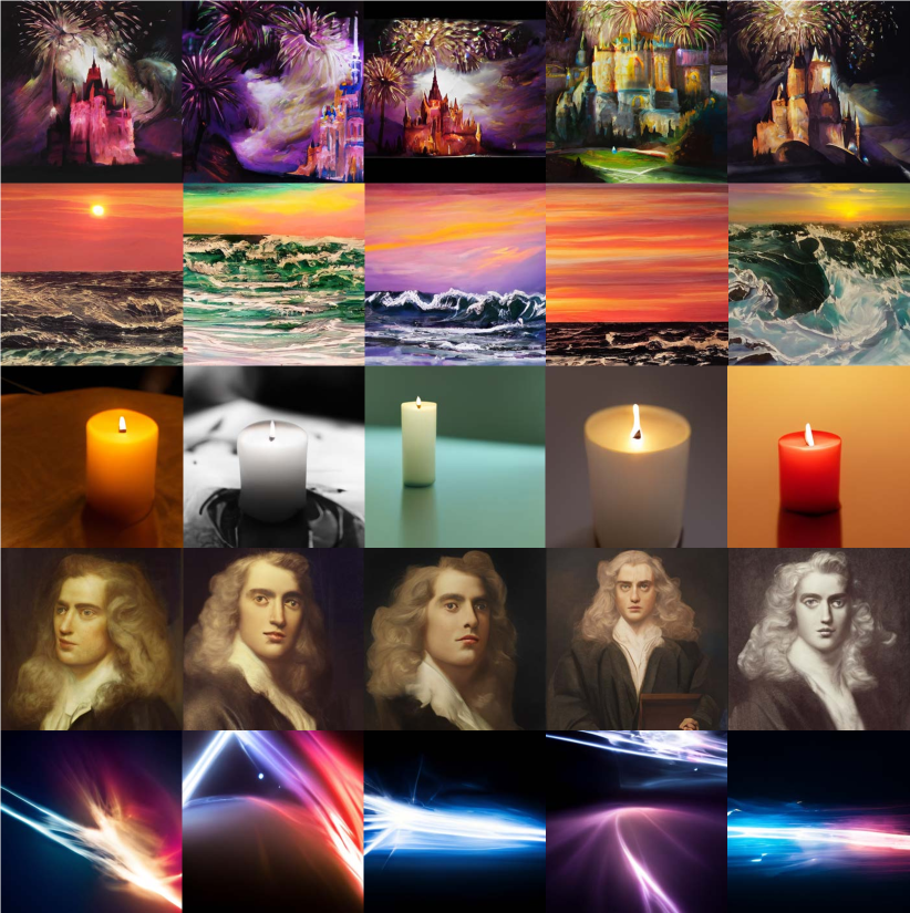
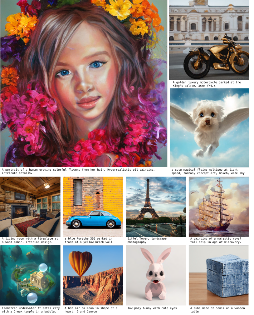
Furthermore, we reintroduce multi-scale training, finding a new scheme that improves image-text alignment and low-frequency details of generated outputs. Multi-scale training allows the GAN-based generator to use parameters in low-resolution blocks more effectively, leading to better image-text alignment and image quality. After careful tuning, we achieve stable and scalable training of a one-billion-parameter GAN (GigaGAN) on large-scale datasets, such as LAION2B-en [88]. Our results are shown in Figure 1.
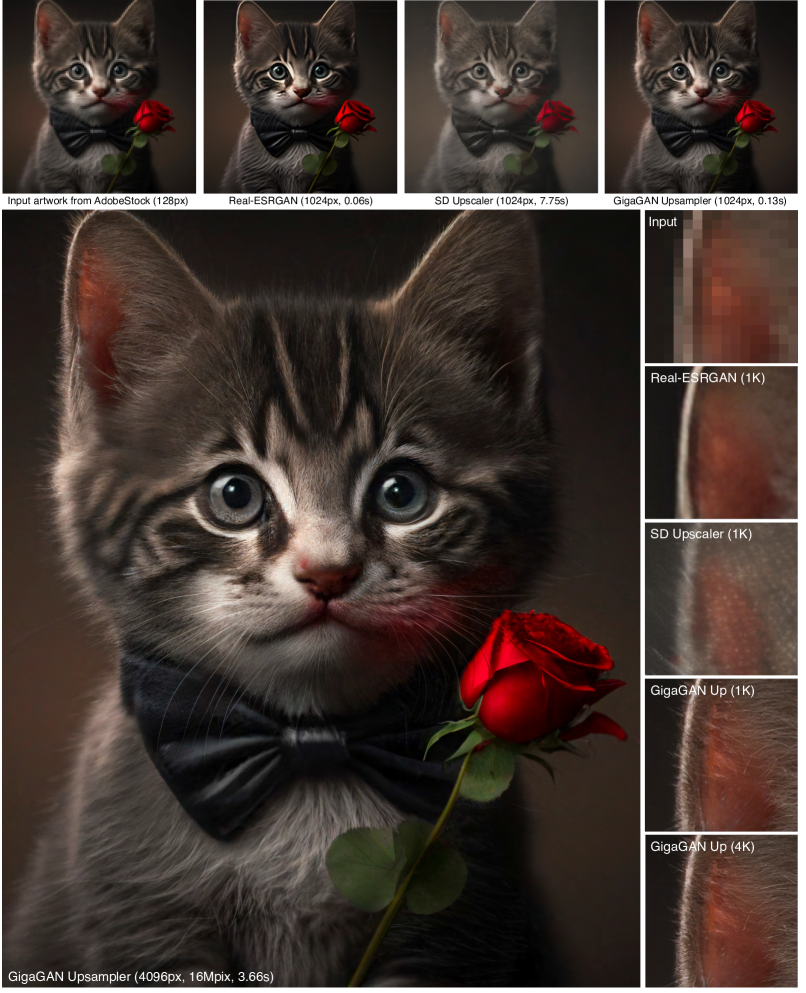
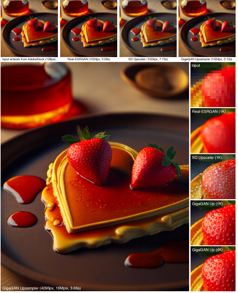
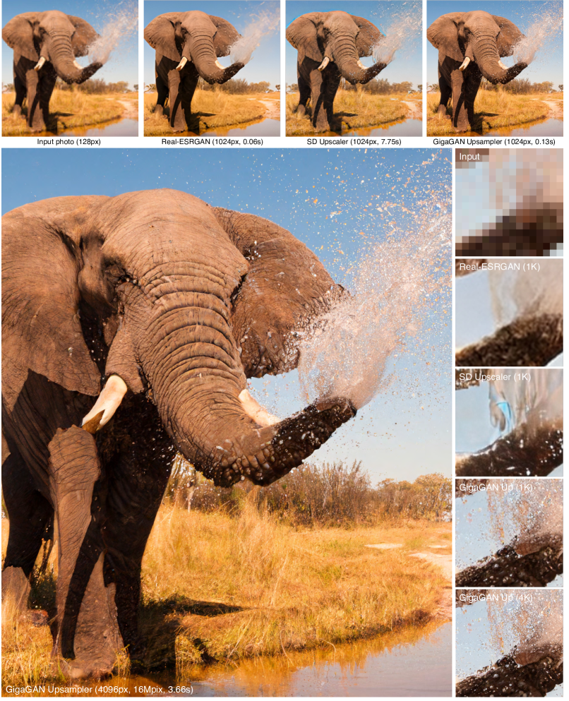
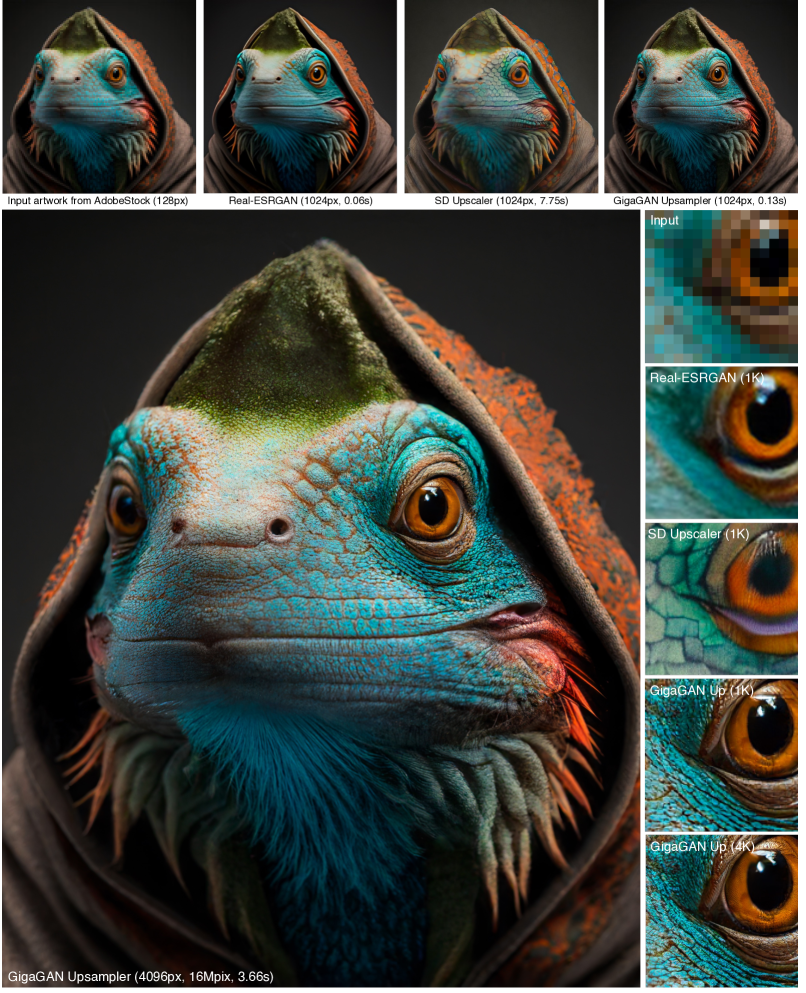
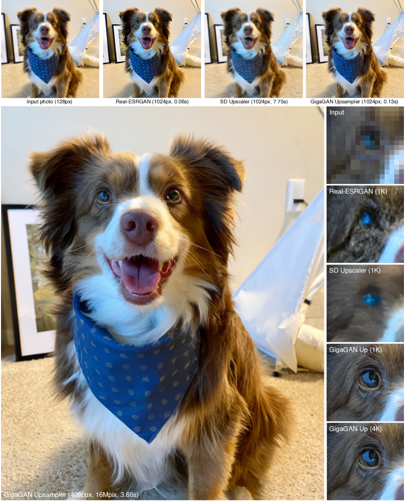
In addition, our method uses a multi-stage approach [14, 104]. We first generate at and then upsample to . These two networks are modular and robust enough to be used in a plug-and-play fashion. We show that our text-conditioned GAN-based upsampling network can be used as an efficient, higher-quality upsampler for a base diffusion model such as DALLE 2, despite never having seen diffusion images at training time (Figures 2).
Together, these advances enable our GigaGAN to go far beyond previous GANs: 36 larger than StyleGAN2 [42] and 6 larger than StyleGAN-XL [86] and XMC-GAN [103]. While our 1B parameter count is still lower than the largest recent synthesis models, such as Imagen (3.0B), DALLE 2 (5.5B), and Parti (20B), we have not yet observed a quality saturation regarding the model size. GigaGAN achieves a zero-shot FID of 9.09 on COCO2014 dataset, lower than the FID of DALLE 2, Parti-750M, and Stable Diffusion.
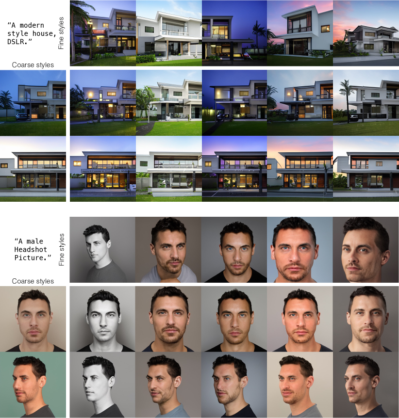
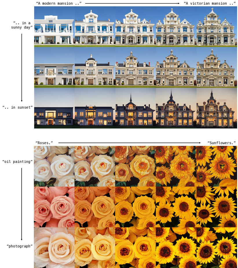
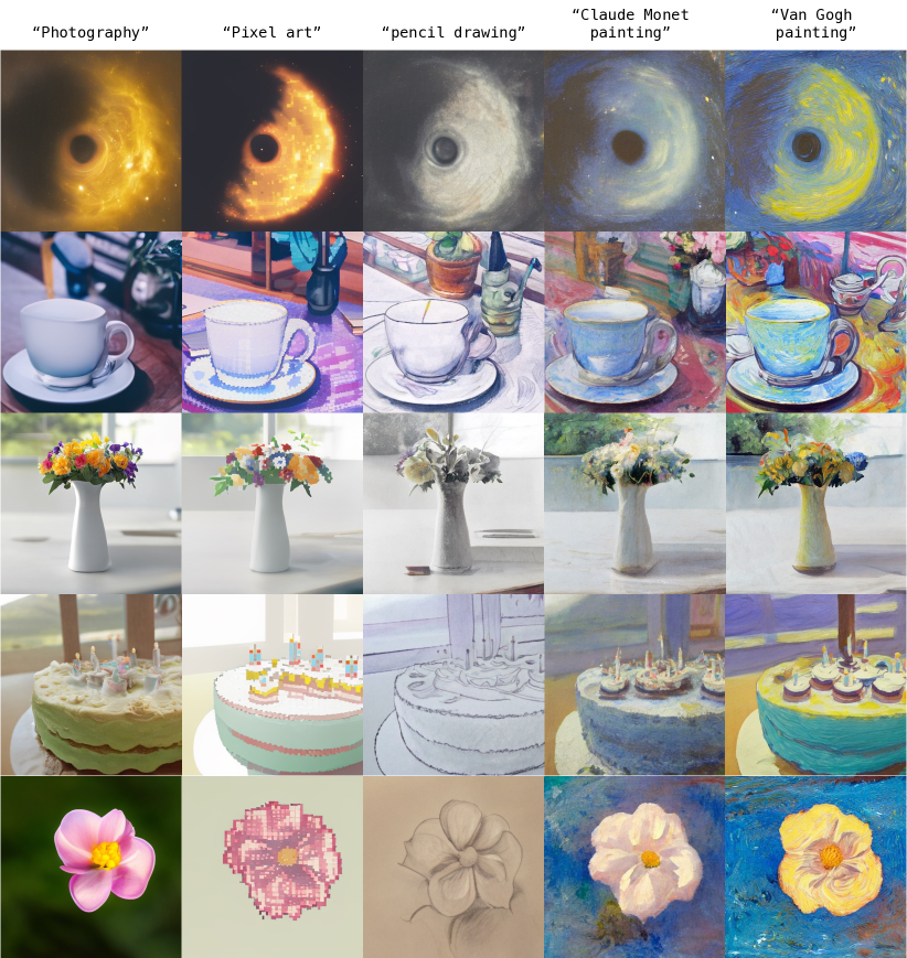
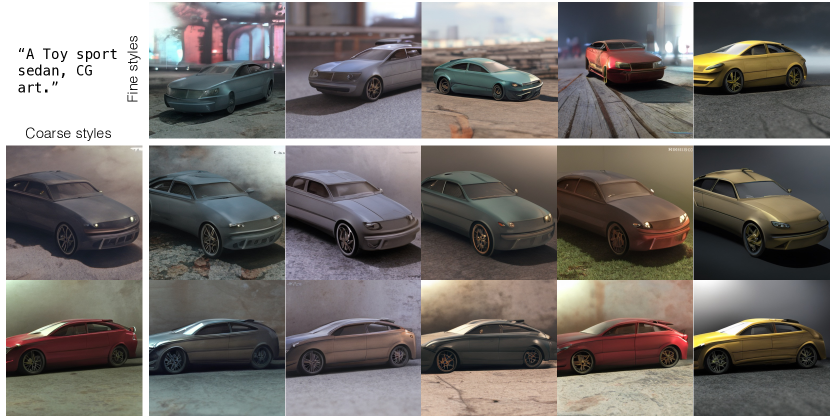
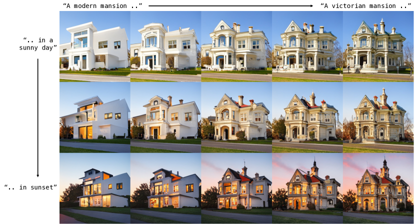
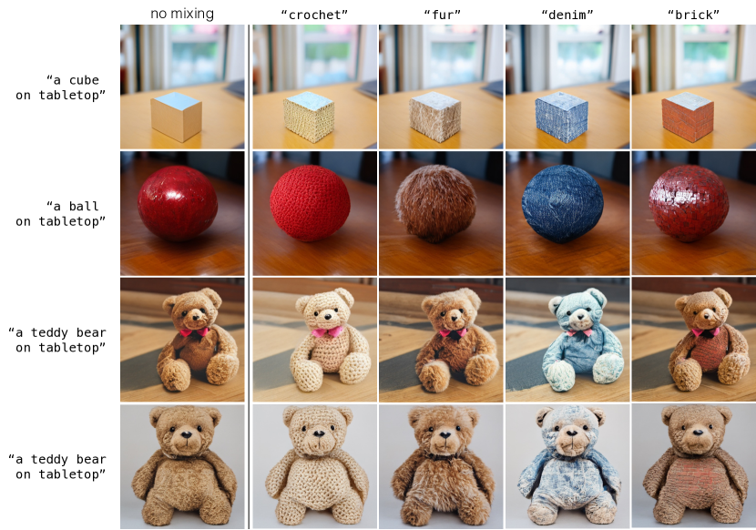
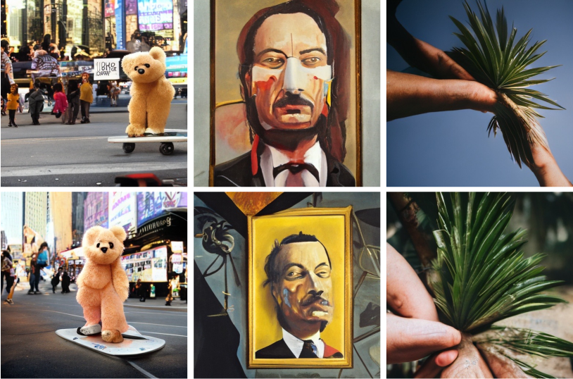
Furthermore, GigaGAN has three major practical advantages compared to diffusion and autoregressive models. First, it is orders of magnitude faster, generating a 512px image in 0.13 seconds (Figure 1). Second, it can synthesize ultra high-res images at 4k resolution in 3.66 seconds. Third, it is endowed with a controllable, latent vector space that lends itself to well-studied controllable image synthesis applications, such as style mixing (Figure 6), prompt interpolation (Figure 7), and prompt mixing (Figure 8).
In summary, our model is the first GAN-based method that successfully trains a billion-scale model on billions of real-world complex Internet images. This suggests that GANs are still a viable option for text-to-image synthesis and should be considered for future aggressive scaling. Please visit our website for additional results.
2 Related Works
Text-to-image synthesis.
Generating a realistic image given a text description, explored by early works [113, 58], is a challenging task. A common approach is text-conditional GANs [77, 76, 104, 99, 111, 93] on specific domains [96] and datasets with a closed-world assumption [54]. With the development of diffusion models [26, 15], autoregressive (AR) transformers [12], and large-scale language encoders [73, 71], text-to-image synthesis has shown remarkable improvement on an open-world of arbitrary text descriptions. GLIDE [63], DALLE 2 [74], and Imagen [80] are representative diffusion models that show photorealistic outputs with the aid of a pretrained language encoder [71, 73]. AR models, such as DALLE [75], Make-A-Scene [20], CogView [16, 17], and Parti [101] also achieve amazing results. While these models exhibit unprecedented image synthesis ability, they require time-consuming iterative processes to achieve high-quality image sampling.
To accelerate the sampling, several methods propose to reduce the sampling steps [59, 83, 89, 57] or reuse pre-computed features [51]. Latent Diffusion Model (LDM) [79] performs the reverse processes in low-dimensional latent space instead of pixel space. However, consecutive reverse processes are still computationally expensive, limiting the usage of large-scale text-to-image models for interactive applications.
GAN-based image synthesis.
GANs [21] have been one of the primary families of generative models for natural image synthesis. As the sampling quality and diversity of GANs improve [72, 39, 41, 42, 40, 44, 84], GANs have been deployed to various computer vision and graphics applications, such as text-to-image synthesis [76], image-to-image translation [34, 110, 29, 49, 66, 65], and image editing [109, 7, 1, 69]. Notably, StyleGAN-family models [42, 40] have shown impressive ability in image synthesis tasks for single-category domains [1, 112, 98, 31, 69]. Other works have explored class-conditional GANs [102, 6, 36, 107, 86] on datasets with a fixed set of object categories.
In this paper, we change the data regimes from single- or multi-categories datasets to extremely data-rich situations. We make the first expedition toward training a large-scale GAN for text-to-image generation on a vast amount of web-crawled text and image pairs, such as LAION2B-en [88] and COYO-700M [8]. Existing GAN-based text-to-image synthesis models [76, 104, 99, 111, 52, 103, 93] are trained on relatively small datasets, such as CUB-200 (12k training pairs), MSCOCO (82k) and LN-OpenImages (507k). Also, those models are evaluated on associated validation datasets, which have not been validated to perform large-scale text-image synthesis like diffusion or AR models.
Super-resolution for large-scale text-to-image models.
Large-scale models require prohibitive computational costs for both training and inference. To reduce the memory and running time, cutting-edge text-to-image models [63, 74, 80, 101] have adopted cascaded generation processes where images are first generated at resolution and upsampled to and sequentially. However, the super-resolution networks are primarily based on diffusion models, which require many iterations. In contrast, our low-res image generators and upsamplers are based on GANs, reducing the computational costs for both stages. Unlike traditional super-resolution techniques [18, 47, 95, 2] that aim to faithfully reproduce low-resolution inputs or handle image degradation like compression artifacts, our upsamplers for large-scale models serve a different purpose. They need to perform larger upsampling factors while potentially leveraging the input text prompt.
3 Method
We train a generator to predict an image given a latent code and text-conditioning signal . We use a discriminator to judge the realism of the generated image, as compared to a sample from the training database , which contains image-text pairs.
Although GANs [39, 41, 6] can successfully generate realistic images on single- and multi-category datasets [41, 100, 13], open-ended text-conditioned synthesis on Internet images remains challenging. We hypothesize that the current limitation stems from its reliance on convolutional layers. That is, the same convolution filters are challenged to model the general image synthesis function for all text conditioning across all locations of the image. In this light, we seek to inject more expressivity into our parameterization by dynamically selecting convolution filters based on the input conditioning and by capturing long-range dependence via the attention mechanism.
Below, we discuss our key contributions to making ConvNets more expressive (Section 3.1), followed by our designs for the generator (Section 3.2) and discriminator (Section 3.3). Lastly, we introduce a new, fast GAN-based upsampler model that can improve the inference quality and speed of our method and diffusion models such as Imagen [80] and DALLE 2 [74].
3.1 Modeling complex contextual interaction
Baseline StyleGAN generator.
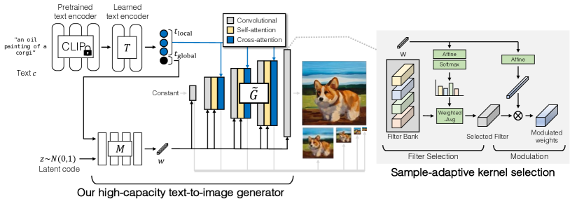
We base our architecture off the conditional version of StyleGAN2 [42], comprised of two networks . The mapping network maps the inputs into a “style” vector , which modulates a series of upsampling convolutional layers in the synthesis network to map a learned constant tensor to an output image . Convolution is the main engine to generate all output pixels, with the vector as the only source of information to model conditioning.
Sample-adaptive kernel selection.
To handle the highly diverse distribution of internet images, we aim to increase the capacity of convolution kernels. However, increasing the width of the convolution layers becomes too demanding, as the same operation is repeated across all locations.
We propose an efficient way to enhance the expressivity of convolutional kernels by creating them on-the-fly based on the text conditioning, as illustrated in Figure 4 (right). In this scheme, we instantiate a bank of filters , instead of one, that takes a feature at each layer. The style vector then goes through an affine layer to predict a set of weights to average across the filters, to produce an aggregated filter .
| (1) |
The filter is then used in the regular convolution pipeline of StyleGAN2, with the second affine layer for weight (de-)modulation [42].
| (2) |
where and represent (de-)modulation and convolution.
At a high level, the softmax-based weighting can be viewed as a differentiable filter selection process based on input conditioning. Furthermore, since the filter selection process is performed only once at each layer, the selection process is much faster than the actual convolution, decoupling compute complexity from the resolution. Our method shares a spirit with dynamic convolutions [35, 97, 23, 91] in that the convolution filters dynamically change per sample, but differs in that we explicitly instantiate a larger filter bank and select weights based on a separate pathway conditional on the -space of StyleGAN.
Interleaving attention with convolution.
Since the convolutional filter operates within its receptive field, it cannot contextualize itself in relationship to distant parts of the images. One way to incorporate such long-range relationships is using attention layers . While recent diffusion-based models [15, 27, 79] have commonly adopted attention mechanisms, StyleGAN architectures are predominantly convolutional with the notable exceptions such as BigGAN [6], GANformer [30], and ViTGAN [50].
We aim to improve the performance of StyleGAN by integrating attention layers with the convolutional backbone. However, simply adding attention layers to StyleGAN often results in training collapse, possibly because the dot-product self-attention is not Lipschitz, as pointed out by Kim et al. [43]. As the Lipschitz continuity of discriminators has played a critical role in stable training [3, 22, 60], we use the L2-distance instead of the dot product as the attention logits to promote Lipschitz continuity [43], similar to ViTGAN [50].
To further improve performance, we find it crucial to match the architectural details of StyleGAN, such as equalized learning rate [39] and weight initialization from a unit normal distribution. We scale down the L2 distance logits to roughly match the unit normal distribution at initialization and reduce the residual gain from the attention layers. We further improve stability by tying the key and query matrix [50], and applying weight decay.
In the synthesis network , the attention layers are interleaved with each convolutional block, leveraging the style vector as an additional token. At each attention block, we add a separate cross-attention mechanism to attend to individual word embeddings [4]. We use each input feature tensor as the query, and the text embeddings as the key and value of the attention mechanism.
3.2 Generator design
Text and latent-code conditioning.
First, we extract the text embedding from the prompt. Previous works [75, 80] have shown that leveraging a strong language model is essential for producing strong results. To do so, we tokenize the input prompt (after padding it to words, following best practices [75, 80]) to produce conditioning vector , and take the features from the penultimate layer [80] of a frozen CLIP feature extractor [71]. To allow for additional flexibility, we apply additional attention layers on top to process the word embeddings before passing them to the MLP-based mapping network. This results in text embedding . Each component of captures the embedding of the word in the sentence. We refer to them as . The EOT (“end of text”) component of aggregates global information, and is called . We process this global text descriptor, along with the latent code , via an MLP mapping network to extract the style .
| (3) |
Different from the original StyleGAN, we use both the text-based style code to modulate the synthesis network and the word embeddings as features for cross-attention.
| (4) |
Synthesis network.
Our synthesis network consists of a series of upsampling convolutional layers, with each layer enhanced with the adaptive kernel selection (Equation 1) and followed by our attention layers.
| (5) |
where , , and denote the -th layer of cross-attention, self-attention, and weight (de-)modulation layers. We find it beneficial to increase the depth of the network by adding more blocks at each layer. In addition, our generator outputs a multi-scale image pyramid with levels, instead of a single image at the highest resolution, similar to MSG-GAN [38] and AnycostGAN [53]. We refer to the pyramid as , with spatial resolutions , respectively. The base level is the output image . Each image of the pyramid is independently used to compute the GAN loss, as discussed in Section 3.3. We follow the findings of StyleGAN-XL [86] and turn off the style mixing and path length regularization [42]. We include more training details in Appendix A.1.
3.3 Discriminator design
As shown in Figure 5, our discriminator consists of separate branches for processing text with the function and images with function . The prediction of real vs. fake is made by comparing the features from the two branches using function . We introduce a new way of making predictions on multiple scales. Finally, we use additional CLIP and Vision-Aided GAN losses [44] to improve stability.
Text conditioning.
First, to incorporate conditioning into discriminators, we extract text descriptor from text . Similar to the generator, we apply a pretrained text encoder, such as CLIP [71], followed by a few learnable attention layers. In this case, we only use the global descriptor.
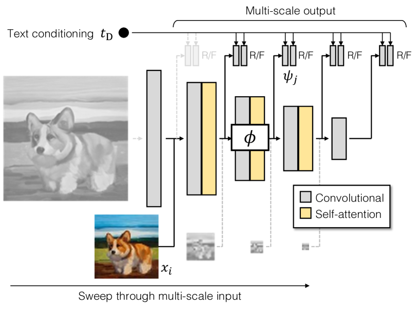
Multiscale image processing.
We observe that the early, low-resolution layers of the generator become inactive, using small dynamic ranges irrespective of the provided prompts. StyleGAN2 [42] also observes this phenomenon, concluding that the network relies on the high-resolution layers, as the model size increases. As recovering performance in low frequencies, which contains complex structure information, is crucial, we redesign the model architecture to provide training signals across multiple scales.
Recall the generator produces a pyramid , with the full image at the pyramid base. MSG-GAN [38] improves performance by making a prediction on the entire pyramid at once, enforcing consistency across scales. However, in our large-scale setting, this harms stability, as this limits the generator from making adjustments to its initial low-res output.
Instead, we process each level of the pyramid independently. As shown in Figure 5, each level makes a real/fake prediction at multiple scales . For example, the full makes predictions at scales, the next level makes predictions at 4 scales, and so on. In total, our discriminator produces predictions, supervising multi-scale generations at multiple scales.
To extract features at different scales, we define feature extractor . Practically, each sub-network is a subset of full , with indicating late entry and indicating early exit. Each layer in is composed of self-attention, followed by convolution with stride 2. The final layer flattens the spatial extent into a tensor. This produces output resolutions at . This allows us to inject lower-resolution images on the pyramid into intermediate layers [39]. As we use a shared feature extractor across different levels and most of the added predictions are made at low resolutions, the increased computation overhead is manageable.
Multi-scale input, multi-scale output adversarial loss.
In total, our training objective consists of discriminator losses, along with our proposed matching loss, to encourage the discriminator to take into account the conditioning:
| (6) |
where is the standard, non-saturating GAN loss [21].
To compute the discriminator output, we train predictor , which uses text feature to modulate image features :
| (7) |
where is implemented as a 4-layer modulated convolution, and is added as a skip connection to explicitly maintain an unconditional prediction branch [62].
Matching-aware loss.
The previous GAN terms measure how closely the image matches the conditioning , as well as how realistic looks, irrespective of conditioning. However, during early training, when artifacts are obvious, the discriminator heavily relies on making a decision independent of conditioning and hesitates to account for the conditioning.
To enforce the discriminator to incorporate conditioning, we match with a random, independently sampled condition , and present them as a fake pair:
| (8) |
CLIP contrastive loss.
We further leverage off-the-shelf pretrained models as a loss function [84, 44, 90]. In particular, we enforce the generator to produce outputs that are identifiable by the pre-trained CLIP image and text encoders [71], and , in the contrastive cross-entropy loss that was used to train them originally.
| (9) |
where are sampled captions from the training data.
Vision-aided adversarial loss.
Lastly, we build an additional discriminator that uses the CLIP model as a backbone, known as Vision-Aided GAN [44]. We freeze the CLIP image encoder, extract features from the intermediate layers, and process them through a simple network with conv layers to make real/fake predictions. We also incorporate conditioning through modulation, as in Equation 7. To stabilize training, we also add a fixed random projection layer, as proposed by Projected GAN [84]. We refer to this as (omitting the learnable discriminator parameters for clarity).
Our final objective is , with weighting between the terms specified in Table A2.
3.4 GAN-based upsampler
Furthermore, GigaGAN framework can be easily extended to train a text-conditioned superresolution model, capable of upsampling the outputs of the base GigaGAN generator to obtain high-resolution images at 512px or 2k resolution. By training our pipeline in two separate stages, we can afford a higher capacity 64px base model within the same computational resources.
In the upsampler, the synthesis network is rearranged to an asymmetric U-Net architecture, which processes the 64px input through 3 downsampling residual blocks, followed by 6 upsampling residual blocks with attention layers to produce the 512px image. There exist skip connections at the same resolution, similar to CoModGAN [106]. The model is trained with the same losses as the base model, as well as the LPIPS Perceptual Loss [105] with respect to the ground truth high-resolution image. Vision-aided GAN is not used for the upsampler. During training and inference time, we apply moderate Gaussian noise augmentation to reduce the gap between real and GAN-generated images. Please refer to Appendix A.3 for more details.
Our GigaGAN framework becomes particularly effective for the superresolution task compared to the diffusion-based models, which cannot afford as many sampling steps as the base model at high resolution. The LPIPS regression loss also provides a stable learning signal. We believe that our GAN upsampler can serve as a drop-in replacement for the superresolution stage of other generative models.
4 Experiments
Systematic, controlled evaluation of large-scale text-to-image synthesis tasks is difficult, as most existing models are not publicly available. Training a new model from scratch would be prohibitively costly, even if the training code were available. Still, we compare our model to recent text-to-image models, such as Imagen [80], Latent Diffusion Models (LDM) [79], Stable Diffusion [78], and Parti [101], based on the available information, while acknowledging considerable differences in the training dataset, number of iterations, batch size, and model size. In addition to text-to-image results, we evaluate our model on ImageNet class-conditional generation in Appendix B, for an apples-to-apples comparison with other methods at a more controlled setting.
For quantitative evaluation, we mainly use the Fréchet Inception Distance (FID) [25] for measuring the realism of the output distribution and the CLIP score for evaluating the image-text alignment.
We conduct five different experiments. First, we show the effectiveness of our method by gradually incorporating each technical component one by one (Section 4.2). Second, our text-to-image synthesis results demonstrate that GigaGAN exhibits comparable FID with Stable Diffusion (SD-v1.5) [79] while generating results hundreds of times faster than diffusion or autoregressive models (Section 4.3). Third, we compare GigaGAN with a distillation-based diffusion model [59] and show that GigaGAN can synthesize higher-quality images faster than the distillation-based diffusion model. Fourth, we verify the advantage of GigaGAN’s upsampler over other upsamplers in both conditional and unconditional super-resolution tasks. Lastly, we show our large-scale GANs still enjoy the continuous and disentangled latent space manipulation of GANs, enabling new image editing modes (Section 4.6).
4.1 Training and evaluation details
We implement GigaGAN based on the StudioGAN PyTorch library [37], following the standard FID evaluation protocol with the anti-aliasing bicubic resize function [67], unless otherwise noted. For text-to-image synthesis, we train our models on the union of LAION2B-en [88] and COYO-700M [8] datasets, with the exception of the 128-to-1024 upsampler model trained on Adobe’s internal Stock images. The image-text pairs are preprocessed based on CLIP score [24], image resolution, and aesthetic score [87], similar to prior work [78]. We use CLIP ViT-L/14 [71] for the pre-trained text encoder and OpenCLIP ViT-G/14 [32] for CLIP score calculation [24] except for Table 1. All our models are trained and evaluated on A100 GPUs. We include more training and evaluation details in Appendix A.
4.2 Effectiveness of proposed components
| Model | FID-10k | CLIP Score | # Param. |
|---|---|---|---|
| StyleGAN2 | 29.91 | 0.222 | 27.8M |
| + Larger (5.7) | 34.07 | 0.223 | 158.9M |
| + Tuned | 28.11 | 0.228 | 26.2M |
| + Attention | 23.87 | 0.235 | 59.0M |
| + Matching-aware D | 27.29 | 0.250 | 59.0M |
| + Matching-aware G and D | 21.66 | 0.254 | 59.0M |
| + Adaptive convolution | 19.97 | 0.261 | 80.2M |
| + Deeper | 19.18 | 0.263 | 161.9M |
| + CLIP loss | 14.88 | 0.280 | 161.9M |
| + Multi-scale training | 14.92 | 0.300 | 164.0M |
| + Vision-aided GAN | 13.67 | 0.287 | 164.0M |
| + Scale-up (GigaGAN) | 9.18 | 0.307 | 652.5M |
First, we show the effectiveness of our formulation via ablation study in Table 1. We set up a baseline by adding text-conditioning to StyleGAN2 and tuning the configuration based on the findings of StyleGAN-XL. We first directly increase the model size of this baseline, but we find that this does not improve the FID and CLIP scores. Then, we add our components one by one and observe that they consistently improve performance. In particular, our model is more scalable, as the higher-capacity version of the final formulation achieves better performance.
4.3 Text-to-Image synthesis
We proceed to train a larger model by increasing the capacity of the base generator and upsampler to 652.5M and 359.1M, respectively. This results in an unprecedented size of GAN model, with a total parameter count of 1.0B. Table 2 compares the performance of our end-to-end pipeline to various text-to-image generative models [75, 63, 79, 74, 80, 5, 101, 108, 78, 10]. Note that there exist differences in the training dataset, the pretrained text encoders, and even image resolutions. For example, GigaGAN initially synthesizes 512px images, which are resized to 256px before evaluation.
Table 2 shows that GigaGAN exhibits a lower FID than DALLE 2 [74], Stable Diffusion [78], and Parti-750M [101]. While our model can be optimized to better match the feature distribution of real images than existing models, the quality of the generated images is not necessarily better (see Appendix C for more samples). We acknowledge that this may represent a corner case of zero-shot FID on COCO2014 dataset and suggest that further research on a better evaluation metric is necessary to improve text-to-image models. Nonetheless, we emphasize that GigaGAN is the first GAN model capable of synthesizing promising images from arbitrary text prompts and exhibits competitive zero-shot FID with other text-to-image models.
| Model | Type | # Param. | # Images | FID-30k | Inf. time | |
|---|---|---|---|---|---|---|
| 256 | GLIDE [63] | Diff | 5.0B | 5.94B | 12.24 | 15.0s |
| LDM [79] | Diff | 1.5B | 0.27B | 12.63 | 9.4s | |
| DALLE 2 [74] | Diff | 5.5B | 5.63B | 10.39 | - | |
| Imagen [80] | Diff | 3.0B | 15.36B | 7.27 | 9.1s | |
| eDiff-I [5] | Diff | 9.1B | 11.47B | 6.95 | 32.0s | |
| DALLE [75] | AR | 12.0B | 1.54B | 27.50 | - | |
| Parti-750M [101] | AR | 750M | 3.69B | 10.71 | - | |
| Parti-3B [101] | AR | 3.0B | 3.69B | 8.10 | 6.4s | |
| Parti-20B [101] | AR | 20.0B | 3.69B | 7.23 | - | |
| LAFITE [108] | GAN | 75M | - | 26.94 | 0.02s | |
| 512 | SD-v1.5∗ [78] | Diff | 0.9B | 3.16B | 9.62 | 2.9s |
| Muse-3B [10] | AR | 3.0B | 0.51B | 7.88 | 1.3s | |
| GigaGAN | GAN | 1.0B | 0.98B | 9.09 | 0.13s |
4.4 Comparison with distilled diffusion models
While GigaGAN is at least 20 times faster than the above diffusion models, there have been efforts to improve the inference speed of diffusion models. We compare GigaGAN with progressively distilled Stable Diffusion (SD-distilled) [59]. Table LABEL:tab:sd_distileed demonstrates that GigaGAN remains faster than the distilled Stable Diffusion while showing better FID and CLIP scores of 21.1 and 0.32, respectively. We follow the evaluation protocol of SD-distilled [59] and report FID and CLIP scores on COCO2017 dataset [54], where images are resized to 512px.
4.5 Super-resolution for large-scale image synthesis
We separately evaluate the performance of the GigaGAN upsampler. Our evaluation consists of two parts. First, we compare GigaGAN with several commonly-used upsamplers. For the text-conditioned upsampling task, we combine the Stable Diffusion [78] 4x Upscaler and 2x Latent Upscaler to establish an 8x upscaling model (SD Upscaler). We also use the unconditional Real-ESRGAN [33] as another baseline. Table 4 measures the performance of the upsampler on random 10K images from the LAION dataset and shows that our GigaGAN upsampler significantly outperforms the other upsamplers in realism scores (FID and patch-FID [9]), text alignment (CLIP score) and closeness to the ground truth (LPIPS [105]). In addition, for more controlled comparison, we train our model on the ImageNet unconditional superresolution task and compare performance with the diffusion-based models, including SR3 [81] and LDM [79]. As shown in Table 5, GigaGAN achieves the best IS and FID scores with a single feedforward pass.
4.6 Controllable image synthesis
StyleGANs are known to possess a linear latent space useful for image manipulation, called the -space. Likewise, we perform coarse and fine-grained style swapping using style vectors . Similar to the -space of StyleGAN, Figure 6 illustrates that GigaGAN maintains a disentangled -space, suggesting existing latent manipulation techniques of StyleGAN can transfer to GigaGAN. Furthermore, our model possesses another latent space of text embedding prior to , and we explore its potential for image synthesis. In Figure 8, we show that the disentangled style manipulation can be controlled via text inputs. In detail, we can compute the text embedding and style code using different prompts and apply them to different layers of the generator. This way, we gain not only the coarse and fine style disentanglement but also an intuitive prompt-based maneuver in the style space.
5 Discussion and Limitations
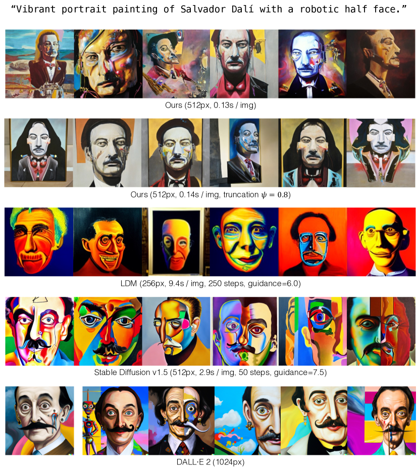
Our experiments provide a conclusive answer about the scalability of GANs: our new architecture can scale up to model sizes that enable text-to-image synthesis. However, the visual quality of our results is not yet comparable to production-grade models like DALLE 2. Figure 9 shows several instances where our method fails to produce high-quality results when compared to DALLE 2, in terms of photorealism and text-to-image alignment for the same input prompts used in their paper.
Nevertheless, we have tested capacities well beyond what is possible with a naïve approach and achieved competitive results with autoregressive and diffusion models trained with similar resources while being orders of magnitude faster and enabling latent interpolation and stylization. Our GigaGAN architecture opens up a whole new design space for large-scale generative models and brings back key editing capabilities that became challenging with the transition to autoregressive and diffusion models. We expect our performance to improve with larger models, as seen in Table 1.
Acknowledgments.
We thank Simon Niklaus, Alexandru Chiculita, and Markus Woodson for building the distributed training pipeline. We thank Nupur Kumari, Gaurav Parmar, Bill Peebles, Phillip Isola, Alyosha Efros, and Joonghyuk Shin for their helpful comments. We also want to thank Chenlin Meng, Chitwan Saharia, and Jiahui Yu for answering many questions about their fantastic work. We thank Kevin Duarte for discussions regarding upsampling beyond 4K. Part of this work was done while Minguk Kang was an intern at Adobe Research. Minguk Kang and Jaesik Park were supported by IITP grant funded by the government of South Korea (MSIT) (POSTECH GSAI: 2019-0-01906 and Image restoration: 2021-0-00537).
References
- [1] Rameen Abdal, Yipeng Qin, and Peter Wonka. Image2stylegan: How to embed images into the stylegan latent space? In IEEE International Conference on Computer Vision (ICCV), 2019.
- [2] Saeed Anwar and Nick Barnes. Densely residual laplacian super-resolution. IEEE Transactions on Pattern Analysis and Machine Intelligence (TPAMI), 2020.
- [3] Martin Arjovsky, Soumith Chintala, and Léon Bottou. Wasserstein Generative Adversarial Networks. In International Conference on Machine Learning (ICML), 2017.
- [4] Dzmitry Bahdanau, Kyunghyun Cho, and Yoshua Bengio. Neural machine translation by jointly learning to align and translate. In International Conference on Learning Representations (ICLR), 2015.
- [5] Yogesh Balaji, Seungjun Nah, Xun Huang, Arash Vahdat, Jiaming Song, Karsten Kreis, Miika Aittala, Timo Aila, Samuli Laine, Bryan Catanzaro, et al. ediffi: Text-to-image diffusion models with an ensemble of expert denoisers. arXiv preprint arXiv:2211.01324, 2022.
- [6] Andrew Brock, Jeff Donahue, and Karen Simonyan. Large Scale GAN Training for High Fidelity Natural Image Synthesis. In International Conference on Learning Representations (ICLR), 2019.
- [7] Andrew Brock, Theodore Lim, James M. Ritchie, and Nick Weston. Neural Photo Editing with Introspective Adversarial Networks. In International Conference on Learning Representations (ICLR), 2017.
- [8] Minwoo Byeon, Beomhee Park, Haecheon Kim, Sungjun Lee, Woonhyuk Baek, and Saehoon Kim. COYO-700M: Image-Text Pair Dataset. https://github.com/kakaobrain/coyo-dataset, 2022.
- [9] Lucy Chai, Michael Gharbi, Eli Shechtman, Phillip Isola, and Richard Zhang. Any-resolution training for high-resolution image synthesis. In European Conference on Computer Vision (ECCV), 2022.
- [10] Huiwen Chang, Han Zhang, Jarred Barber, AJ Maschinot, Jose Lezama, Lu Jiang, Ming-Hsuan Yang, Kevin Murphy, William T Freeman, Michael Rubinstein, et al. Muse: Text-to-image generation via masked generative transformers. arXiv preprint arXiv:2301.00704, 2023.
- [11] Huiwen Chang, Han Zhang, Lu Jiang, Ce Liu, and William T Freeman. Maskgit: Masked generative image transformer. In IEEE Conference on Computer Vision and Pattern Recognition (CVPR), pages 11315–11325, 2022.
- [12] Mark Chen, Alec Radford, Rewon Child, Jeffrey Wu, Heewoo Jun, David Luan, and Ilya Sutskever. Generative pretraining from pixels. In International Conference on Machine Learning (ICML). PMLR, 2020.
- [13] Jia Deng, Wei Dong, Richard Socher, Li-Jia Li, Kai Li, and Li Fei-Fei. Imagenet: A large-scale hierarchical image database. In IEEE Conference on Computer Vision and Pattern Recognition (CVPR), 2009.
- [14] Emily L Denton, Soumith Chintala, Rob Fergus, et al. Deep generative image models using a laplacian pyramid of adversarial networks. Conference on Neural Information Processing Systems (NeurIPS), 28, 2015.
- [15] Prafulla Dhariwal and Alexander Nichol. Diffusion models beat gans on image synthesis. In Conference on Neural Information Processing Systems (NeurIPS), 2021.
- [16] Ming Ding, Zhuoyi Yang, Wenyi Hong, Wendi Zheng, Chang Zhou, Da Yin, Junyang Lin, Xu Zou, Zhou Shao, Hongxia Yang, et al. Cogview: Mastering text-to-image generation via transformers. In Conference on Neural Information Processing Systems (NeurIPS), 2021.
- [17] Ming Ding, Wendi Zheng, Wenyi Hong, and Jie Tang. Cogview2: Faster and better text-to-image generation via hierarchical transformers. arXiv preprint arXiv:2204.14217, 2022.
- [18] Chao Dong, Chen Change Loy, Kaiming He, and Xiaoou Tang. Image super-resolution using deep convolutional networks. IEEE Transactions on Pattern Analysis and Machine Intelligence (TPAMI), 2015.
- [19] Patrick Esser, Robin Rombach, and Bjorn Ommer. Taming transformers for high-resolution image synthesis. In IEEE Conference on Computer Vision and Pattern Recognition (CVPR), pages 12873–12883, 2021.
- [20] Oran Gafni, Adam Polyak, Oron Ashual, Shelly Sheynin, Devi Parikh, and Yaniv Taigman. Make-A-Scene: Scene-Based Text-to-Image Generation with Human Priors. In European Conference on Computer Vision (ECCV), 2022.
- [21] Ian Goodfellow, Jean Pouget-Abadie, Mehdi Mirza, Bing Xu, David Warde-Farley, Sherjil Ozair, Aaron Courville, and Yoshua Bengio. Generative Adversarial Nets. In Conference on Neural Information Processing Systems (NeurIPS), pages 2672–2680, 2014.
- [22] Ishaan Gulrajani, Faruk Ahmed, Martin Arjovsky, Vincent Dumoulin, and Aaron C Courville. Improved training of wasserstein gans. In Conference on Neural Information Processing Systems (NeurIPS), 2017.
- [23] David Ha, Andrew Dai, and Quoc V Le. Hypernetworks. In International Conference on Learning Representations (ICLR), 2017.
- [24] Jack Hessel, Ari Holtzman, Maxwell Forbes, Ronan Le Bras, and Yejin Choi. Clipscore: A reference-free evaluation metric for image captioning. arXiv preprint arXiv:2104.08718, 2021.
- [25] Martin Heusel, Hubert Ramsauer, Thomas Unterthiner, Bernhard Nessler, and Sepp Hochreiter. GANs Trained by a Two Time-Scale Update Rule Converge to a Local Nash Equilibrium. In Conference on Neural Information Processing Systems (NeurIPS), pages 6626–6637, 2017.
- [26] Jonathan Ho, Ajay Jain, and P. Abbeel. Denoising Diffusion Probabilistic Models. In Conference on Neural Information Processing Systems (NeurIPS), 2020.
- [27] Jonathan Ho, Chitwan Saharia, William Chan, David J. Fleet, Mohammad Norouzi, and Tim Salimans. Cascaded Diffusion Models for High Fidelity Image Generation. Journal of Machine Learning Research, pages 47:1–47:33, 2022.
- [28] Jonathan Ho and Tim Salimans. Classifier-free diffusion guidance. In Conference on Neural Information Processing Systems (NeurIPS) Workshop, 2022.
- [29] Xun Huang, Ming-Yu Liu, Serge Belongie, and Jan Kautz. Multimodal unsupervised image-to-image translation. In European Conference on Computer Vision (ECCV), 2018.
- [30] Drew A Hudson and Larry Zitnick. Generative adversarial transformers. In International Conference on Machine Learning (ICML), 2021.
- [31] Erik Härkönen, Aaron Hertzmann, Jaakko Lehtinen, and Sylvain Paris. GANSpace: Discovering Interpretable GAN Controls. In Conference on Neural Information Processing Systems (NeurIPS), 2020.
- [32] Gabriel Ilharco, Mitchell Wortsman, Ross Wightman, Cade Gordon, Nicholas Carlini, Rohan Taori, Achal Dave, Vaishaal Shankar, Hongseok Namkoong, John Miller, Hannaneh Hajishirzi, Ali Farhadi, and Ludwig Schmidt. Openclip. https://doi.org/10.5281/zenodo.5143773, 2021.
- [33] intao Wang and Liangbin Xie and Chao Dong and Ying Shan. Real-esrgan: Training real-world blind super-resolution with pure synthetic data. In IEEE International Conference on Computer Vision (ICCV) Workshop, 2021.
- [34] Phillip Isola, Jun-Yan Zhu, Tinghui Zhou, and Alexei A Efros. Image-to-image translation with conditional adversarial networks. In IEEE Conference on Computer Vision and Pattern Recognition (CVPR), 2017.
- [35] Xu Jia, Bert De Brabandere, Tinne Tuytelaars, and Luc V Gool. Dynamic filter networks. Conference on Neural Information Processing Systems (NeurIPS), 29, 2016.
- [36] Minguk Kang, Woohyeon Shim, Minsu Cho, and Jaesik Park. Rebooting ACGAN: Auxiliary Classifier GANs with Stable Training. In Conference on Neural Information Processing Systems (NeurIPS), 2021.
- [37] Minguk Kang, Joonghyuk Shin, and Jaesik Park. StudioGAN: A Taxonomy and Benchmark of GANs for Image Synthesis. arXiv preprint arXiv:2206.09479, 2022.
- [38] Animesh Karnewar and Oliver Wang. Msg-gan: Multi-scale gradients for generative adversarial networks. In IEEE Conference on Computer Vision and Pattern Recognition (CVPR), pages 7799–7808, 2020.
- [39] Tero Karras, Timo Aila, Samuli Laine, and Jaakko Lehtinen. Progressive growing of gans for improved quality, stability, and variation. In International Conference on Learning Representations (ICLR), 2018.
- [40] Tero Karras, Miika Aittala, Samuli Laine, Erik Härkönen, Janne Hellsten, Jaakko Lehtinen, and Timo Aila. Alias-free generative adversarial networks. In Conference on Neural Information Processing Systems (NeurIPS), 2021.
- [41] Tero Karras, Samuli Laine, and Timo Aila. A style-based generator architecture for generative adversarial networks. In IEEE Conference on Computer Vision and Pattern Recognition (CVPR), pages 4401–4410, 2019.
- [42] Tero Karras, Samuli Laine, Miika Aittala, Janne Hellsten, Jaakko Lehtinen, and Timo Aila. Analyzing and improving the image quality of stylegan. In IEEE Conference on Computer Vision and Pattern Recognition (CVPR), pages 8110–8119, 2020.
- [43] Hyunjik Kim, George Papamakarios, and Andriy Mnih. The lipschitz constant of self-attention. In International Conference on Machine Learning (ICML), 2021.
- [44] Nupur Kumari, Richard Zhang, Eli Shechtman, and Jun-Yan Zhu. Ensembling off-the-shelf models for gan training. In IEEE Conference on Computer Vision and Pattern Recognition (CVPR), 2022.
- [45] Tuomas Kynkäänniemi, Tero Karras, Miika Aittala, Timo Aila, and Jaakko Lehtinen. The Role of ImageNet Classes in Fr’echet Inception Distance. arXiv preprint arXiv:2203.06026, 2022.
- [46] Tuomas Kynkäänniemi, Tero Karras, Samuli Laine, Jaakko Lehtinen, and Timo Aila. Improved Precision and Recall Metric for Assessing Generative Models. In Conference on Neural Information Processing Systems (NeurIPS), 2019.
- [47] Christian Ledig, Lucas Theis, Ferenc Huszár, Jose Caballero, Andrew Cunningham, Alejandro Acosta, Andrew Aitken, Alykhan Tejani, Johannes Totz, Zehan Wang, et al. Photo-realistic single image super-resolution using a generative adversarial network. In IEEE Conference on Computer Vision and Pattern Recognition (CVPR), 2017.
- [48] Doyup Lee, Chiheon Kim, Saehoon Kim, Minsu Cho, and Wook-Shin Han. Autoregressive Image Generation using Residual Quantization. In IEEE Conference on Computer Vision and Pattern Recognition (CVPR), pages 11523–11532, 2022.
- [49] Hsin-Ying Lee, Hung-Yu Tseng, Jia-Bin Huang, Maneesh Singh, and Ming-Hsuan Yang. Diverse image-to-image translation via disentangled representations. In European Conference on Computer Vision (ECCV), 2018.
- [50] Kwonjoon Lee, Huiwen Chang, Lu Jiang, Han Zhang, Zhuowen Tu, and Ce Liu. ViTGAN: Training GANs with vision transformers. In International Conference on Learning Representations (ICLR), 2022.
- [51] Muyang Li, Ji Lin, Chenlin Meng, Stefano Ermon, Song Han, and Jun-Yan Zhu. Efficient spatially sparse inference for conditional gans and diffusion models. In Conference on Neural Information Processing Systems (NeurIPS), 2022.
- [52] Jiadong Liang, Wenjie Pei, and Feng Lu. Cpgan: Content-parsing generative adversarial networks for text-to-image synthesis. In European Conference on Computer Vision (ECCV), 2020.
- [53] Ji Lin, Richard Zhang, Frieder Ganz, Song Han, and Jun-Yan Zhu. Anycost gans for interactive image synthesis and editing. In IEEE Conference on Computer Vision and Pattern Recognition (CVPR), pages 14986–14996, 2021.
- [54] Tsung-Yi Lin, Michael Maire, Serge Belongie, James Hays, Pietro Perona, Deva Ramanan, Piotr Dollár, and C Lawrence Zitnick. Microsoft coco: Common objects in context. In European Conference on Computer Vision (ECCV), 2014.
- [55] Luping Liu, Yi Ren, Zhijie Lin, and Zhou Zhao. Pseudo Numerical Methods for Diffusion Models on Manifolds. In International Conference on Learning Representations (ICLR), 2022.
- [56] Ilya Loshchilov and Frank Hutter. Decoupled Weight Decay Regularization. In International Conference on Learning Representations (ICLR), 2019.
- [57] Cheng Lu, Yuhao Zhou, Fan Bao, Jianfei Chen, Chongxuan Li, and Jun Zhu. Dpm-solver: A fast ode solver for diffusion probabilistic model sampling in around 10 steps. arXiv preprint arXiv:2206.00927, 2022.
- [58] Elman Mansimov, Emilio Parisotto, Jimmy Lei Ba, and Ruslan Salakhutdinov. Generating Images from Captions with Attention. In International Conference on Learning Representations (ICLR), 2016.
- [59] Chenlin Meng, Ruiqi Gao, Diederik P Kingma, Stefano Ermon, Jonathan Ho, and Tim Salimans. On distillation of guided diffusion models. In Conference on Neural Information Processing Systems (NeurIPS) Workshop, 2022.
- [60] Lars Mescheder, Andreas Geiger, and Sebastian Nowozin. Which training methods for gans do actually converge? In International Conference on Machine Learning (ICML), 2018.
- [61] Lars Mescheder, Sebastian Nowozin, and Andreas Geiger. Which Training Methods for GANs do actually Converge? In International Conference on Machine Learning (ICML), 2018.
- [62] Takeru Miyato and Masanori Koyama. cGANs with Projection Discriminator. In International Conference on Learning Representations (ICLR), 2018.
- [63] Alex Nichol, Prafulla Dhariwal, Aditya Ramesh, Pranav Shyam, Pamela Mishkin, Bob McGrew, Ilya Sutskever, and Mark Chen. GLIDE: Towards Photorealistic Image Generation and Editing with Text-Guided Diffusion Models. In International Conference on Machine Learning (ICML), 2022.
- [64] OpenAI. DALL·E API. https://openai.com/product/dall-e-2, 2022.
- [65] Taesung Park, Alexei A. Efros, Richard Zhang, and Jun-Yan Zhu. Contrastive Learning for Unpaired Image-to-Image Translation. In European Conference on Computer Vision (ECCV), 2020.
- [66] Taesung Park, Ming-Yu Liu, Ting-Chun Wang, and Jun-Yan Zhu. Semantic image synthesis with spatially-adaptive normalization. In IEEE Conference on Computer Vision and Pattern Recognition (CVPR), 2019.
- [67] Gaurav Parmar, Richard Zhang, and Jun-Yan Zhu. On Aliased Resizing and Surprising Subtleties in GAN Evaluation. In IEEE Conference on Computer Vision and Pattern Recognition (CVPR), 2022.
- [68] Adam Paszke, Sam Gross, Francisco Massa, Adam Lerer, James Bradbury, Gregory Chanan, Trevor Killeen, Zeming Lin, Natalia Gimelshein, Luca Antiga, Alban Desmaison, Andreas Kopf, Edward Yang, Zachary DeVito, Martin Raison, Alykhan Tejani, Sasank Chilamkurthy, Benoit Steiner, Lu Fang, Junjie Bai, and Soumith Chintala. PyTorch: An Imperative Style, High-Performance Deep Learning Library. In Conference on Neural Information Processing Systems (NeurIPS), pages 8024–8035, 2019.
- [69] Or Patashnik, Zongze Wu, Eli Shechtman, Daniel Cohen-Or, and Dani Lischinski. Styleclip: Text-driven manipulation of stylegan imagery. In IEEE International Conference on Computer Vision (ICCV), 2021.
- [70] William Peebles and Saining Xie. Scalable Diffusion Models with Transformers. arXiv preprint arXiv:2212.09748, 2022.
- [71] Alec Radford, Jong Wook Kim, Chris Hallacy, Aditya Ramesh, Gabriel Goh, Sandhini Agarwal, Girish Sastry, Amanda Askell, Pamela Mishkin, Jack Clark, et al. Learning transferable visual models from natural language supervision. In International Conference on Machine Learning (ICML), 2021.
- [72] Alec Radford, Luke Metz, and Soumith Chintala. Unsupervised representation learning with deep convolutional generative adversarial networks. arXiv preprint arXiv:1511.06434, 2015.
- [73] Colin Raffel, Noam Shazeer, Adam Roberts, Katherine Lee, Sharan Narang, Michael Matena, Yanqi Zhou, Wei Li, and Peter J. Liu. Exploring the Limits of Transfer Learning with a Unified Text-to-Text Transformer. Journal of Machine Learning Research, 2020.
- [74] Aditya Ramesh, Prafulla Dhariwal, Alex Nichol, Casey Chu, and Mark Chen. Hierarchical text-conditional image generation with clip latents. arXiv preprint arXiv:2204.06125, 2022.
- [75] Aditya Ramesh, Mikhail Pavlov, Gabriel Goh, Scott Gray, Chelsea Voss, Alec Radford, Mark Chen, and Ilya Sutskever. Zero-shot text-to-image generation. In International Conference on Machine Learning (ICML), 2021.
- [76] Scott Reed, Zeynep Akata, Xinchen Yan, Lajanugen Logeswaran, Bernt Schiele, and Honglak Lee. Generative adversarial text to image synthesis. In International Conference on Machine Learning (ICML), 2016.
- [77] Scott E Reed, Zeynep Akata, Santosh Mohan, Samuel Tenka, Bernt Schiele, and Honglak Lee. Learning what and where to draw. In Conference on Neural Information Processing Systems (NeurIPS), 2016.
- [78] Robin Rombach, Andreas Blattmann, Dominik Lorenz, Patrick Esser, and Björn Ommer. Stable Diffusion. https://github.com/CompVis/stable-diffusion. Accessed: 2022-11-06.
- [79] Robin Rombach, Andreas Blattmann, Dominik Lorenz, Patrick Esser, and Björn Ommer. High-resolution image synthesis with latent diffusion models. In IEEE Conference on Computer Vision and Pattern Recognition (CVPR), 2022.
- [80] Chitwan Saharia, William Chan, Saurabh Saxena, Lala Li, Jay Whang, Emily Denton, Seyed Kamyar Seyed Ghasemipour, Burcu Karagol Ayan, S Sara Mahdavi, Rapha Gontijo Lopes, et al. Photorealistic Text-to-Image Diffusion Models with Deep Language Understanding. arXiv preprint arXiv:2205.11487, 2022.
- [81] Chitwan Saharia, Jonathan Ho, William Chan, Tim Salimans, David J Fleet, and Mohammad Norouzi. Image super-resolution via iterative refinement. IEEE Transactions on Pattern Analysis and Machine Intelligence (TPAMI), 2022.
- [82] Tim Salimans, Ian Goodfellow, Wojciech Zaremba, Vicki Cheung, Alec Radford, Xi Chen, and Xi Chen. Improved Techniques for Training GANs. In Conference on Neural Information Processing Systems (NeurIPS), pages 2234–2242, 2016.
- [83] Tim Salimans and Jonathan Ho. Progressive distillation for fast sampling of diffusion models. In International Conference on Learning Representations (ICLR), 2022.
- [84] Axel Sauer, Kashyap Chitta, Jens Müller, and Andreas Geiger. Projected GANs Converge Faster. In Conference on Neural Information Processing Systems (NeurIPS), 2021.
- [85] Axel Sauer, Tero Karras, Samuli Laine, Andreas Geiger, and Timo Aila. StyleGAN-T: Unlocking the Power of GANs for Fast Large-Scale Text-to-Image Synthesis. arXiv preprint arXiv:2301.09515, 2023.
- [86] Axel Sauer, Katja Schwarz, and Andreas Geiger. Stylegan-xl: Scaling stylegan to large diverse datasets. In ACM SIGGRAPH 2022 Conference Proceedings, pages 1–10, 2022.
- [87] Christoph Schuhmann. CLIP+MLP Aesthetic Score Predictor. https://github.com/christophschuhmann/improved-aesthetic-predictor.
- [88] Christoph Schuhmann, Romain Beaumont, Richard Vencu, Cade Gordon, Ross Wightman, Mehdi Cherti, Theo Coombes, Aarush Katta, Clayton Mullis, Mitchell Wortsman, et al. LAION-5B: An open large-scale dataset for training next generation image-text models. arXiv preprint arXiv:2210.08402, 2022.
- [89] Jiaming Song, Chenlin Meng, and Stefano Ermon. Denoising Diffusion Implicit Models. In International Conference on Learning Representations (ICLR), 2021.
- [90] Diana Sungatullina, Egor Zakharov, Dmitry Ulyanov, and Victor Lempitsky. Image manipulation with perceptual discriminators. In European Conference on Computer Vision (ECCV), 2018.
- [91] Md Mehrab Tanjim. DynamicRec: a dynamic convolutional network for next item recommendation. In Proceedings of the 29th ACM International Conference on Information and Knowledge Management (CIKM), 2020.
- [92] Ming Tao, Bing-Kun Bao, Hao Tang, and Changsheng Xu. GALIP: Generative Adversarial CLIPs for Text-to-Image Synthesis. arXiv preprint arXiv:2301.12959, 2023.
- [93] Ming Tao, Hao Tang, Fei Wu, Xiao-Yuan Jing, Bing-Kun Bao, and Changsheng Xu. DF-GAN: A Simple and Effective Baseline for Text-to-Image Synthesis. In IEEE Conference on Computer Vision and Pattern Recognition (CVPR), 2022.
- [94] Ken Turkowski. Filters for common resampling tasks. Graphics gems, pages 147–165, 1990.
- [95] Xintao Wang, Ke Yu, Shixiang Wu, Jinjin Gu, Yihao Liu, Chao Dong, Yu Qiao, and Chen Change Loy. Esrgan: Enhanced super-resolution generative adversarial networks. In European Conference on Computer Vision (ECCV) Workshop, 2018.
- [96] P. Welinder, S. Branson, T. Mita, C. Wah, F. Schroff, S. Belongie, and P. Perona. Caltech-UCSD Birds 200. Technical report, California Institute of Technology, 2010.
- [97] Felix Wu, Angela Fan, Alexei Baevski, Yann Dauphin, and Michael Auli. Pay Less Attention with Lightweight and Dynamic Convolutions. In International Conference on Learning Representations (ICLR), 2018.
- [98] Jonas Wulff and Antonio Torralba. Improving inversion and generation diversity in stylegan using a gaussianized latent space. arXiv preprint arXiv:2009.06529, 2020.
- [99] Tao Xu, Pengchuan Zhang, Qiuyuan Huang, Han Zhang, Zhe Gan, Xiaolei Huang, and Xiaodong He. Attngan: Fine-grained text to image generation with attentional generative adversarial networks. In IEEE Conference on Computer Vision and Pattern Recognition (CVPR), 2018.
- [100] Fisher Yu, Ari Seff, Yinda Zhang, Shuran Song, Thomas Funkhouser, and Jianxiong Xiao. Lsun: Construction of a large-scale image dataset using deep learning with humans in the loop. arXiv preprint arXiv:1506.03365, 2015.
- [101] Jiahui Yu, Yuanzhong Xu, Jing Yu Koh, Thang Luong, Gunjan Baid, Zirui Wang, Vijay Vasudevan, Alexander Ku, Yinfei Yang, Burcu Karagol Ayan, et al. Scaling autoregressive models for content-rich text-to-image generation. arXiv preprint arXiv:2206.10789, 2022.
- [102] Han Zhang, Ian Goodfellow, Dimitris Metaxas, and Augustus Odena. Self-Attention Generative Adversarial Networks. In International Conference on Machine Learning (ICML), pages 7354–7363, 2019.
- [103] Han Zhang, Jing Yu Koh, Jason Baldridge, Honglak Lee, and Yinfei Yang. Cross-Modal Contrastive Learning for Text-to-Image Generation. In IEEE Conference on Computer Vision and Pattern Recognition (CVPR), 2021.
- [104] Han Zhang, Tao Xu, Hongsheng Li, Shaoting Zhang, Xiaogang Wang, Xiaolei Huang, and Dimitris N Metaxas. Stackgan: Text to photo-realistic image synthesis with stacked generative adversarial networks. In IEEE International Conference on Computer Vision (ICCV), 2017.
- [105] Richard Zhang, Phillip Isola, Alexei A Efros, Eli Shechtman, and Oliver Wang. The unreasonable effectiveness of deep features as a perceptual metric. In IEEE Conference on Computer Vision and Pattern Recognition (CVPR), 2018.
- [106] Shengyu Zhao, Jonathan Cui, Yilun Sheng, Yue Dong, Xiao Liang, Eric I Chang, and Yan Xu. Large Scale Image Completion via Co-Modulated Generative Adversarial Networks. In International Conference on Learning Representations (ICLR), 2021.
- [107] Shengyu Zhao, Zhijian Liu, Ji Lin, Jun-Yan Zhu, and Song Han. Differentiable augmentation for data-efficient gan training. arXiv preprint arXiv 2006.10738, 2020.
- [108] Yufan Zhou, Ruiyi Zhang, Changyou Chen, Chunyuan Li, Chris Tensmeyer, Tong Yu, Jiuxiang Gu, Jinhui Xu, and Tong Sun. Lafite: Towards language-free training for text-to-image generation. In IEEE Conference on Computer Vision and Pattern Recognition (CVPR), 2022.
- [109] Jun-Yan Zhu, Philipp Krähenbühl, Eli Shechtman, and Alexei A Efros. Generative visual manipulation on the natural image manifold. In European Conference on Computer Vision (ECCV), 2016.
- [110] Jun-Yan Zhu, Taesung Park, Phillip Isola, and Alexei A Efros. Unpaired image-to-image translation using cycle-consistent adversarial networks. In IEEE International Conference on Computer Vision (ICCV), pages 2223–2232, 2017.
- [111] Minfeng Zhu, Pingbo Pan, Wei Chen, and Yi Yang. Dm-gan: Dynamic memory generative adversarial networks for text-to-image synthesis. In IEEE Conference on Computer Vision and Pattern Recognition (CVPR), 2019.
- [112] Peihao Zhu, Rameen Abdal, Yipeng Qin, John Femiani, and Peter Wonka. Improved stylegan embedding: Where are the good latents? arXiv preprint arXiv:2012.09036, 2020.
- [113] Xiaojin Zhu, Andrew B Goldberg, Mohamed Eldawy, Charles R Dyer, and Bradley Strock. A text-to-picture synthesis system for augmenting communication. In The AAAI Conference on Artificial Intelligence, 2007.
Appendices
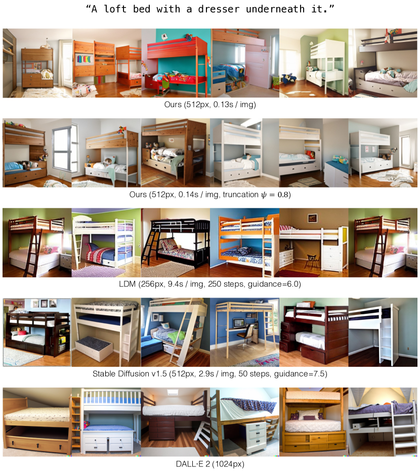
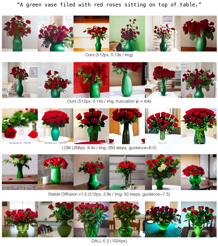
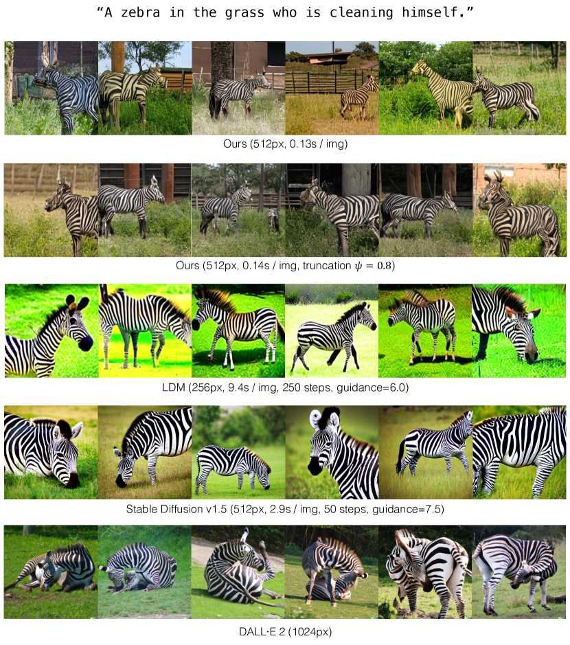
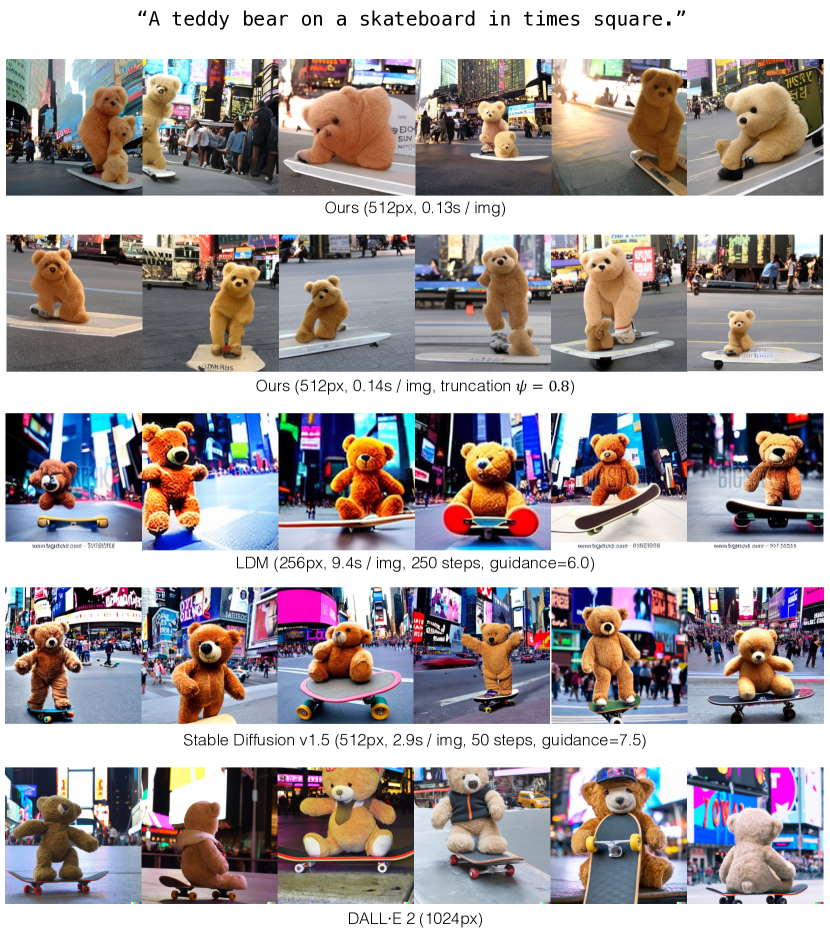
We first provide training and evaluation details in Appendix A. Then, we share results on ImageNet, with visual comparison to existing methods in Appendix B. Lastly in Appendix C, we show more visuals on our text-to-image synthesis results and compare them with LDM [79], Stable Diffusion [78], and DALLE 2 [74].
Appendix A Training and evaluation details
A.1 Text-to-image synthesis
We train GigaGAN on a combined dataset of LAION2B-en [88] and COYO-700M [8] in PyTorch framework [68]. For training, we apply center cropping, which results in a square image whose length is the same as the shorter side of the original image. Then, we resize the image to the resolution using PIL.LANCZOS [94] resizer, which supports anti-aliasing [67]. We filter the training image–text pairs based on image resolution (), CLIP score () [24], aesthetics score () [87], and remove watermarked images. We train our GigaGAN based on the configurations denoted in the fourth and fifth columns of Table A2.
For evaluation, we use 40,504 and 30,000 real and generated images from COCO2014 [54] validation dataset as described in Imagen [80]. We apply the center cropping and resize the real and generated images to resolution using PIL.BICUBIC, suggested by clean-fid [67]. We use the clean-fid library [67] for FID calculation.
A.2 Conditional image synthesis on ImageNet
We follow the training and evaluation protocol proposed by Kang et al. [37] to make a fair comparison against other cutting-edge generative models. We use the same cropping strategy to process images for training and evaluation as in our text-to-image experiments. Then, we resize the image to the target resolution ( for the base generator or for the super-resolution stack) using PIL.LANCZOS [94] resizer, which supports anti-aliasing [67]. Using the pre-processed training images, we train GigaGAN based on the configurations denoted in the second and third columns of Table A2.
For evaluation, we upsample the real and generated images to resolution using the PIL.BICUBIC resizer. To compute FID, we generate 50k images without truncation tricks [41, 6] and compare those images with the entire training dataset. We use the pre-calculated features of real images provided by StudioGAN [37] and 50k generated images for Precision & Recall [46] calculation.
A.3 Super-resolution results
Appendix B ImageNet experiments
B.1 Qualitative results
We train a class-conditional GAN on the ImageNet dataset [13], for which apples-to-apples comparison is possible using the same dataset and evaluation pipeline. Our GAN achieves comparable generation quality to the cutting-edge generative models without a pretrained ImageNet classifier, which acts favorably toward automated metrics [45]. We apply L2 self-attention, style-adaptive convolution kernel, and matching-aware loss to our model and use a wider synthesis network to train the base 64px model with a batch size of 1024. Additionally, we train a separate 256px class-conditional upsampler model and combine them with an end-to-end finetuning stage. Table A1 shows that our method generates high-fidelity images.
| Model | IS [82] | FID [25] | Precision/Recall [46] | Size | |
|---|---|---|---|---|---|
| GAN | BigGAN-Deep[6] | 224.46 | 6.95 | 0.89/0.38 | 112M |
| StyleGAN-XL[86] | 297.62 | 2.32 | 0.82/0.61 | 166M | |
| Diffusion | ADM-G[15] | 207.86 | 4.48 | 0.84/0.62 | 608M |
| ADM-G-U[15] | 240.24 | 4.01 | 0.85/0.62 | 726M | |
| CDM[27] | 158.71 | 4.88 | - / - | - | |
| LDM-8-G[79] | 209.52 | 7.76 | - / - | 506M | |
| LDM-4-G[79] | 247.67 | 3.60 | - / - | 400M | |
| DiT-XL/2†[70] | 278.24 | 2.27 | - / - | 675M | |
| xformer | Mask-GIT[11] | 216.38 | 5.40 | 0.87/0.60 | 227M |
| VQ-GAN[19] | 314.61 | 5.20 | 0.81/0.57 | 1.4B | |
| RQ-Transformer[48] | 339.41 | 3.83 | 0.85/0.60 | 3.8B | |
| GigaGAN | 225.52 | 3.45 | 0.84/0.61 | 569M |
B.2 Quantitative results
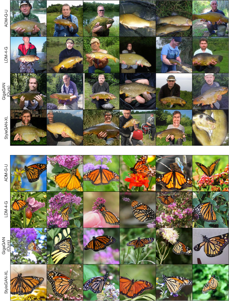
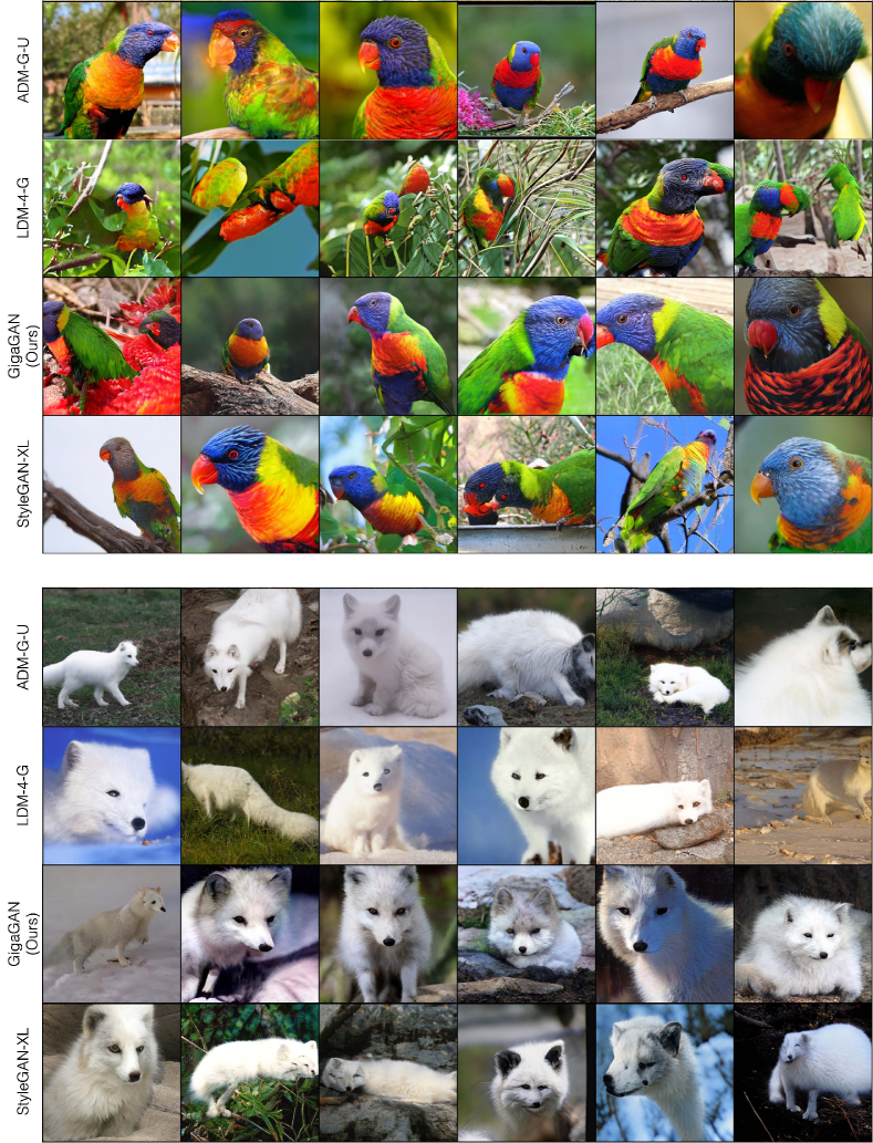
We provide visual results from ADM-G-U, LDM, StyleGAN-XL [86], and GigaGAN in Figures A1 and A2. Although StyleGAN-XL has the lowest FID, its visual quality appears worse than ADM and GigaGAN. StyleGAN-XL struggles to synthesize the overall image structure, leading to less realistic images. In contrast, GigaGAN appears to synthesize the overall structure better than StyleGAN-XL and faithfully captures fine-grained details, such as the wing patterns of a monarch and the white fur of an arctic fox. Compared to GigaGAN, ADM-G-U synthesizes the image structure more rationally but lacks in reflecting the aforementioned fine-grained details.
| Task | Class-Label-to-Image | Text-to-Image | Super-Resolution | ||
| Dataset Resolution | ImageNet 64 | ImageNet 64256 | LAIONCOYO 64 | LAIONCOYO 64512 | ImageNet 64256 |
| dimension | 64 | 128 | 128 | 128 | 128 |
| dimension | 512 | 512 | 1024 | 512 | 512 |
| Adversarial loss type | Logistic | Logistic | Logistic | Logistic | Logistic |
| Conditioning loss type | PD | PD | MS-I/O | MS-I/O | - |
| R1 strength | 0.2048 | 0.2048 | 0.2048 2.048 | 0.2048 | 0.2048 |
| R1 interval | 16 | 16 | 16 | 16 | 16 |
| G Matching loss strength | - | - | 1.0 | 1.0 | - |
| D Matching loss strength | - | - | 1.0 | 1.0 | - |
| LPIPS strength | - | 100.0 | - | 10.0 | 100.0 |
| CLIP loss strength | - | - | 0.2 1.0 | 1.0 | - |
| Optimizer | AdamW | AdamW | AdamW | AdamW | AdamW |
| Batch size | 1024 | 256 | 5121024 | 192320 | 256 |
| learning rate | 0.0025 | 0.0025 | 0.0025 | 0.0025 | 0.0025 |
| learning rate | 0.0025 | 0.0025 | 0.0025 | 0.0025 | 0.0025 |
| for AdamW | 0.0 | 0.0 | 0.0 | 0.0 | 0.0 |
| for AdamW | 0.99 | 0.99 | 0.99 | 0.99 | 0.99 |
| Weight decay strength | 0.00001 | 0.00001 | 0.00001 | 0.00001 | 0.00001 |
| Weight decay strength on attention | - | - | 0.01 | 0.01 | - |
| updates per update | 1 | 1 | 1 | 1 | 1 |
| G ema beta | 0.9651 | 0.9912 | 0.9999 | 0.9890 | 0.9912 |
| Precision | TF32 | TF32 | TF32 | TF32 | TF32 |
| Mapping Network layer depth | 2 | 4 | 4 | 4 | 4 |
| Text Transformer layer depth | - | - | 4 | 2 | - |
| channel base | 32768 | 32768 | 16384 | 32768 | 32768 |
| channel base | 32768 | 32768 | 16384 | 32768 | 32768 |
| channel max | 512 | 512 | 1600 | 512 | 512 |
| channel max | 768 | 512 | 1536 | 512 | 512 |
| G of filters for adaptive kernel selection | 8 | 4 | [1, 1, 2, 4, 8] | [1, 1, 1, 1, 1, 2, 4, 8, 16, 16, 16, 16] | 4 |
| Attention type | self | self | self + cross | self + cross | self |
| attention resolutions | [8, 16, 32] | [16, 32] | [8, 16, 32] | [8, 16, 32, 64] | [16, 32] |
| attention resolutions | [8, 16, 32] | - | [8, 16, 32] | [8, 16] | - |
| attention depth | [4, 4, 4] | [4, 2] | [2, 2, 1] | [2, 2, 2, 1] | [4, 2] |
| attention depth | [1, 1, 1] | - | [2, 2, 1] | [2, 2] | - |
| Attention dimension multiplier | 1.0 | 1.4 | 1.0 | 1.0 | 1.4 |
| MLP dimension multiplier of attention | 4.0 | 4.0 | 4.0 | 4.0 | 4.0 |
| synthesis block per resolution | 1 | 5 | [3, 3, 3, 2, 2] | [4, 4, 4, 4, 4, 4, 3] | 5 |
| discriminator block per resolution | 1 | 1 | [1, 2, 2, 2, 2] | 1 | - |
| Residual gain | 1.0 | 0.4 | 0.4 | 0.4 | 0.4 |
| Residual gain on attention | 1.0 | 0.3 | 0.3 | 0.5 | 0.3 |
| MinibatchStdLayer | True | True | False | True | True |
| D epilogue mbstd group size | 8 | 4 | - | 2 | 4 |
| Multi-scale training | False | False | True | True | False |
| Multi-scale loss ratio (high to low res) | - | - | [0.33, 0.17, 0.17, 0.17, 0.17] | - | |
| D intermediate layer adv loss weight | - | - | 0.01 | [0.2, 0.2, 0.1, 0.1, 0.1, 0.1, 0.1, 0.1] | - |
| D intermediate layer matching loss weight | - | - | 0.05 | - | - |
| Vision-aided discriminator backbone | - | - | CLIP-ViT-B/32-V | - | - |
| Model size | 209.5M | 359.8M | 652.5M | 359.1M | 359.0M |
| Model size | 76.7M | 30.7M | 381.4M | 130.1M | 28.9M |
| Iterations | 300k | 620k | 1350k | 915k | 160k |
| A100 GPUs for training | 64 | 64 | 96128 | 64 | 32 |
Appendix C Text-to-image synthesis results
C.1 Truncation trick at inference
Similar to the classifier guidance [15] and classifier-free guidance [28] used in diffusion models such as LDM, our GAN model can leverage the truncation trick [6, 41] at inference time.
| (9) |
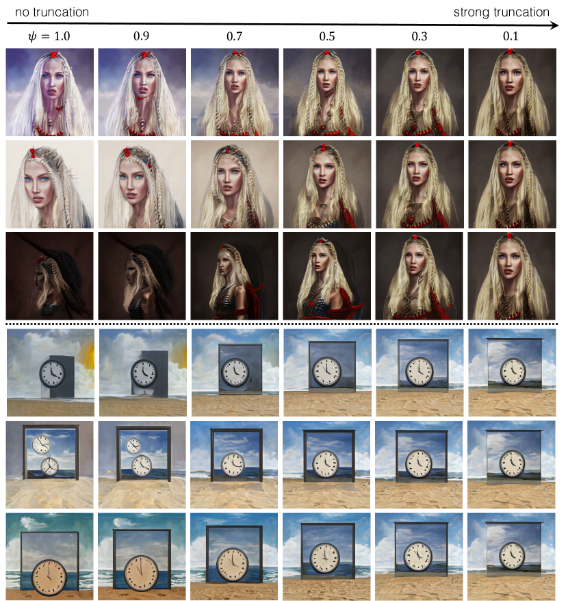
where is the mean of of the entire dataset, which can be precomputed. In essence, the truncation trick lets us trade diversity for fidelity by interpolating the latent vector to the mean of the distribution and thereby making the outputs more typical. When , is not used, and there is no truncation. When , collapses to the mean, losing diversity.
While it is straightforward to apply the truncation trick for the unconditional case, it is less clear how to achieve this for text-conditional image generation. We find that interpolating the latent vector toward both the mean of the entire distribution as well as the mean of conditioned on the text prompt produces desirable results.
| (10) |
where can be computed at inference time by sampling 16 times with the same , and taking the average. This operation’s overhead is negligible, as the mapping network is computationally light compared to the synthesis network. At , becomes , meaning no truncation. Figure A4 demonstrates the effect of our text-conditioned truncation trick.
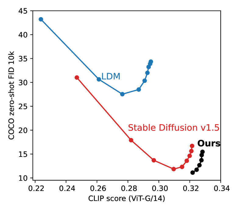
Quantitatively, the effect of truncation is similar to the guidance technique of diffusion models. As shown in Figure A3, the CLIP score increases with more truncation, where the FID increases due to reduced diversity.
C.2 Comparison to diffusion models
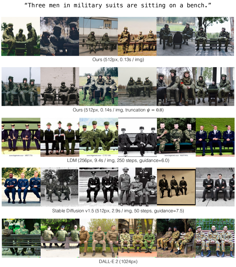
Finally, we show randomly sampled results of our model and compare them with publicly available diffusion models, LDM [79], Stable Diffusion [78], and DALLE 2 [74].